Time-Aware Tensor Decomposition for Missing Entry Prediction

Abstract

Given a time-evolving tensor with missing entries, how can we effectively factorize it for precisely predicting the missing entries? Tensor factorization has been extensively utilized for analyzing various multi-dimensional real-world data. However, existing models for tensor factorization have disregarded the temporal property for tensor factorization while most real-world data are closely related to time. Moreover, they do not address accuracy degradation due to the sparsity of time slices. The essential problems of how to exploit the temporal property for tensor decomposition and consider the sparsity of time slices remain unresolved.

In this paper, we propose TATD (Time-Aware Tensor Decomposition), a novel tensor decomposition method for real-world temporal tensors. TATD is designed to exploit temporal dependency and time-varying sparsity of real-world temporal tensors. We propose a new smoothing regularization with Gaussian kernel for modeling time dependency. Moreover, we improve the performance of TATD by considering time-varying sparsity. We design an alternating optimization scheme suitable for temporal tensor factorization with our smoothing regularization. Extensive experiments show that TATD provides the state-of-the-art accuracy for decomposing temporal tensors.

1 Introduction

Given a temporal tensor where one mode denotes time, how can we discover its latent factors for effectively predicting missing entries? A tensor, or multi-dimensional array, has been widely used to model multi-faceted relationships for time-evolving data. For example, air quality data (Zhang et al. 2017) containing measurements of contaminants collected from sensors at every time step are modeled as a 3-mode temporal tensor (time, site, contaminant). Tensor factorization is a fundamental building block for effectively analyzing tensors by revealing latent factors between entities (Kolda and Sun 2008; Kang et al. 2012; Bahadori et al. 2014; Oh et al. 2018; Park et al. 2017; Liu et al. 2019), and it has been extensively utilized in various real-world applications across diverse domains including recommender systems (Symeonidis 2016), clustering (Sun et al. 2015), anomaly detection (Kolda and Sun 2008), correlation analysis (Sun et al. 2006), network forensic (Maruhashi et al. 2011), and latent concept discovery (Kolda et al. 2005). CANDECOMP/PARAFAC (CP) (Harshman et al. 1970) factorization is one of the most widely used tensor factorization models, which factorizes a tensor into a set of factor matrices and a core tensor which is restricted to be diagonal (Harshman et al. 1970).

Previous CP factorization methods (Kolda and Sun 2008; Kang et al. 2012; Bahadori et al. 2014; Oh et al. 2018; Park et al. 2017; Liu et al. 2019; Symeonidis 2016; Kolda et al. 2005; Sun et al. 2006; Maruhashi et al. 2011; Sun et al. 2015) do not consider temporal property when it comes to factorizing tensors while most time-evolving tensors exhibit temporal dependency. Recently, few studies (Wu et al. 2019; Yu et al. 2016) have been conducted to address the above problem, but they consider only the past information of a time step to model temporal dependencies. A model needs to examine both the past and the future information to capture accurate temporal properties since information at each time point is heavily related to that in the past and the future. In addition, they do not consider the time-varying sparsity, one of the main properties in temporal tensors. The main challenges to design an accurate temporal tensor factorization method for missing entry prediction are 1) how to harness the time dependency in real-world data, and 2) how to exploit the varying sparsity of temporal slices.

In this paper, we propose TATD (Time-Aware Tensor Decomposition), a time-aware tensor factorization method for analyzing real-world temporal tensors. Our main observation is that adjacent time factor vectors are mostly similar to each other since time slices in a temporal tensor are closely related to each other. Based on this observation, TATD employs a kernel smoothing regularization to make time factor vectors reflect temporal dependency. Moreover, TATD imposes a time-dependent sparsity penalty to strengthen the smoothing regularization. The sparsity penalty modulates the amount of the regularization using the sparsity of time slices. TATD further improves accuracy using an effective alternating optimization scheme that incorporates an analytical solution and Adam optimizer. Through extensive experiments, we show that TATD effectively considers the time dependency for tensor factorization, and achieves higher accuracy compared to existing methods. Our main contributions are as follows:

Method. We propose TATD, a novel tensor factorization method considering temporal dependency. TATD exploits a smoothing regularization for effectively modeling time factor with time dependency, and adjusts it by utilizing a time-varying sparsity.

Optimization. We propose an alternating optimization strategy suitable for our smoothing regularization. The strategy alternatively optimizes factor matrices with an analytical solution and Adam optimizer.

Performance. Extensive experiments show that exploiting temporal dependency is crucial for accurate tensor factorization of temporal tensors. TATD achieves up to $7.01\times$ lower RMSE and $5.50\times$ lower MAE for sparse tensor factorization compared to the second best methods.

The rest of the paper is organized as follows. In Section 2, we explain preliminaries on tensor factorization. Section 3 describes our proposed method TATD. We demonstrate our experimental results in Section 4. After reviewing related work in Section 5, we conclude in Section 6.

Table 1: Table of symbols

Symbol	Definition
$\boldsymbol{\mathscr{X}}$	input tensor $\in\mathbf{R}^{I_{1}\times...\times I_{N}}$
$\alpha$	index $(i_{1},...,i_{N})$ of $\boldsymbol{\mathscr{X}}$
$x_{\alpha}$	entry of $\boldsymbol{\mathscr{X}}$ with index $\alpha$
$N$	order of tensor $\boldsymbol{\mathscr{X}}$
$I_{n}$	length of the $n$th mode of tensor $\boldsymbol{\mathscr{X}}$
$\mathbf{A}^{(n)}$	$n$th factor matrix $(\in\mathbf{R}^{I_{n}\times K})$
$\mathbf{a}^{(n)}_{i_{n}}$	$i_{n}$th row of $\mathbf{A}^{(n)}$
$a^{(n)}_{i_{n}k}$	$(i_{n},k)$th entry of $\mathbf{A}^{(n)}$
$K$	rank of tensor $\boldsymbol{\mathscr{X}}$
$t$	time mode of $\boldsymbol{\mathscr{X}}$
$\boldsymbol{\mathscr{X}}_{i_{t}}$	$i_{t}$th time slice of size $I_{1}\times\cdots\times I_{t-1}\times I_{t+1}\cdots\times I_{N}$
$\omega_{i_{t}}$	number of observed entries of time slice $\boldsymbol{\mathscr{X}}_{i_{t}}$
$\|\boldsymbol{\mathscr{X}}\|_{F}$	Frobenius norm of tensor $\boldsymbol{\mathscr{X}}$
$\lambda_{t}$, $\lambda_{r}$	regularization parameter

2 Preliminaries

We describe the preliminaries of tensor and tensor decomposition. We use the symbols listed in Table 1.

2.1 Tensor and Notations

Tensors are defined as multi-dimensional arrays that generalize the one-dimensional arrays (or vectors) and two-dimensional arrays (or matrices) to higher dimensions. Specifically, the dimension of a tensor is referred to as order or way; the length of each mode is called ‘dimensionality’ and denoted by $I_{1},\cdots,I_{n}$. We use boldface Euler script letters (e.g., $\boldsymbol{\mathscr{X}}$) to denote tensors, boldface capitals (e.g., $\mathbf{A}$) to denote matrices, and boldface lower cases (e.g., $\mathbf{a}$) to denote vectors. The $\alpha=(i_{1},\cdots,i_{N})$th entry of tensor $\boldsymbol{\mathscr{X}}$ is denoted by $x_{\alpha}$.

A slice of a 3-order tensor is a two-dimensional subset of it. There are the horizontal, lateral, and frontal slices in a 3-order tensor $\boldsymbol{\mathscr{X}}$, denoted by $\mathbf{X}_{i_{1}::}$, $\mathbf{X}_{:i_{2}:}$, and $\mathbf{X}_{::i_{3}}$. A tensor containing a mode representing time is called a temporal tensor.

A time slice in a $3$-mode temporal tensor represents a two-dimensional subset disjointed by each time index. For example, $\mathbf{X}_{i_{t}::}$ is an $i_{t}$th time slice when the first mode is the time mode. For brevity, we express $\mathbf{X}_{i_{t}::}$ as $\mathbf{X}_{i_{t}}$. Our proposed method is not limited to a $3$-mode tensor so that a time slice in an N-order temporal tensor corresponds to an (N-1)-dimensional subset of the tensor sliced by each time index. We formally define a time slice $\boldsymbol{\mathscr{X}}_{i_{t}}$ as follows:

Definition 1 (Time slice $\boldsymbol{\mathscr{X}}_{i_{t}}$)

Given an $N$-order tensor $\boldsymbol{\mathscr{X}}\in\mathbb{R}^{I_{1}\times\cdots\times I_{N}}$ and a time mode $t$, we extract time slices of size $I_{1}\times\cdots\times I_{t-1}\times I_{t+1}\cdots\times I_{N}$ by slicing the tensor $\boldsymbol{\mathscr{X}}$ so that an $i_{t}$th time slice $\boldsymbol{\mathscr{X}}_{i_{t}}\in\mathbb{R}^{I_{1}\times\cdots\times I_{t-1}\times I_{t+1}\cdots\times I_{N}}$ is an $N-1$ order tensor obtained at time $i_{t}$ where $1\leq i_{t}\leq I_{t}$. $\square$

The Frobenius norm of a tensor $\boldsymbol{\mathscr{X}}$ $(\in\mathbf{R}^{I_{1}\times...\times I_{N}})$ is given by $||\boldsymbol{\mathscr{X}}||_{F}=\sqrt{\sum_{\alpha\in\Omega}{\boldsymbol{\mathscr{X}}^{2}_{\alpha}}}$, where $\Omega$ is the set of indices of entries in $\boldsymbol{\mathscr{X}}$, $\alpha\ =(i_{1},\cdots,i_{N})$ is an index included in $\Omega$, and $\boldsymbol{\mathscr{X}}_{\alpha}$ is the $(i_{1},\cdots,i_{N})$th entry of the tensor $\boldsymbol{\mathscr{X}}$.

2.2 Tensor Decomposition

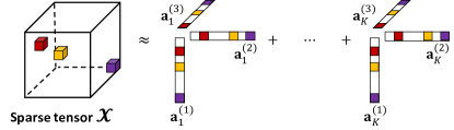
Figure 1: CP decomposition of a 3-way sparse tensor into $K$ components

We provide the definition of CP decomposition (Harshman et al. 1970; Kiers 2000) which is one of the most representative factorization models. Fig. 1 illustrates CP decomposition of a $3$-way sparse tensor. Our model TATD is based on CP decomposition.

Definition 2 (CP decomposition)

Given a rank $K$ and an $N$-mode tensor $\boldsymbol{\mathscr{X}}\in\mathbb{R}^{I_{1}\times\cdots\times I_{N}}$ with observed entries, CP decomposition approximates $\boldsymbol{\mathscr{X}}$ by finding latent factor matrices $\{\mathbf{A}^{(n)}\in\mathbb{R}^{I_{n}\times K}\>|\>1\leq n\leq N\}$. The factor matrices are obtained by minimizing the following loss function:

$$\boldsymbol{\mathscr{L}}\left(\mathbf{A}^{(1)},\cdots,\mathbf{A}^{(N)}\right) =\sum_{\forall\alpha\in\Omega}{\left({x}_{\alpha}-\sum_{k=1}^{K}\prod_{n=1}^{N}a^{(n)}_{i_{n}k}\right)^{2}}$$ (1)

where $\Omega$ indicates the set of the indices of the observed entries, $x_{\alpha}$ indicates the $\alpha=(i_{1},\cdots,i_{N})$th entry of $\boldsymbol{\mathscr{X}}$, and $a^{(n)}_{i_{n}k}$ indicates $(i_{n},k)$th entry of $\mathbf{A}^{(n)}$. $\square$

The standard CP decomposition method is not specifically designed to deal with temporal dependency; thus CP decomposition does not give an enough accuracy for predicting missing values in a temporal tensor. Although a few methods (Yu et al. 2016; Wu et al. 2019) have tried to capture temporal interaction, none of them 1) captures temporal dependency between adjacent time steps, and 2) exploits the sparsity of temporal slices. Our proposed TATD carefully captures temporal information and considers sparsity of temporal slices for better accuracy in decomposing temporal tensors.

3 Proposed Method

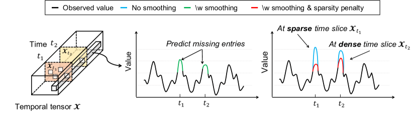
Figure 2: Illustration of a smoothing regularization and sparsity penalty by TATD. TATD accurately predicts missing entries of time slices at $t_{1}$ and $t_{2}$ with the smoothing regularization. Also, TATD adjusts the amount of the smoothing regularization according to the time-varying sparsity. For a sparse time slice at $t_{1}$, TATD predicts its missing entries via strong regularization to actively consider nearby slices. For a dense time slice at $t_{2}$, TATD predicts its missing entries with weak regularization by paying little attention to nearby slices

In this section, we propose TATD (Time-Aware Tensor Decomposition), a tensor factorization method for temporal tensors. We first introduce the overview of TATD in Section 3.1. We then explain the details of TATD in Sections 3.2 and 3.3, and the optimization technique in Section 3.4.

3.1 Overview

TATD is a tensor factorization method designed for temporal tensors with missing entries. There are several challenges in designing an accurate tensor factorization method for temporal tensors.

1. Model temporal dependency. Temporal dependency is an essential structure of temporal tensor. How can we design a tensor factorization model to reflect the temporal dependency?

2. Exploit sparsity of time slices. Time-evolving tensor has varying sparsity for its temporal slices. How can we exploit the temporal sparsity for better accuracy?

3. Optimization. How can we efficiently train our model and minimize its loss function?

To overcome the aforementioned challenges, we propose the following main ideas.

1. Smoothing regularization (Section 3.2). We propose a smoothing regularization on time factor to capture temporal dependency.

2. Time-dependent sparsity penalty (Section 3.3). We propose a time-dependent sparsity penalty to further improve the accuracy.

3. Careful optimization (Section 3.4). We propose an optimization strategy utilizing an analytical solution and Adam optimizer to efficiently and accurately train our model.

Fig. 2 illustrates overview of TATD. We observe that adjacent time slices in a temporal tensor are closely related with each other due to temporal trend of the tensor. Based on the observation, TATD uses smoothing regularization such that time factor vectors for adjacent time slices become similar. We also observe that different time slices have different densities. Instead of applying the same amount of regularization for all the time slices, we control the amount of regularization based on the sparsity of time slices such that sparse slices are affected more from the regularization. It is also crucial to efficiently optimize our objective function. We propose an optimization strategy exploiting alternating minimization to expedite training and improve the accuracy.

3.2 Smoothing Regularization

We describe how we formulate the smoothing regularization on tensor decomposition to capture temporal dependency. Our main observation is that temporal tensors have temporal trends, and adjacent time slices are closely related. For example, consider an air quality tensor containing measurements of pollutant at a specific time and location; it is modeled as a 3-mode tensor $\boldsymbol{\mathscr{X}}$ (time, location, type of pollutants; measurements). Since the amount of pollutants at nearby time steps are closely related, the time slice $\boldsymbol{\mathscr{X}}_{t}$ at time $t$ is closely related to the time slices $\boldsymbol{\mathscr{X}}_{t-1}$ at time $t-1$ and $\boldsymbol{\mathscr{X}}_{t+1}$ at time $t+1$. This implies the time factor matrix after tensor decomposition should have related rows for adjacent time steps.

Based on the observation, our objective function is as follows. Given an $N$-order temporal tensor $\boldsymbol{\mathscr{X}}\in\mathbb{R}^{I_{1}\times\cdots\times I_{N}}$ with observed entries $\Omega$, the time mode $t$, and a window size $S$, we find factor matrices $\mathbf{A}^{(n)}\in\mathbb{R}^{I_{n}\times K}$ $,1\leq n\leq N$ that minimizes

$$\boldsymbol{\mathscr{L}}=\sum_{\alpha\in\Omega}{\left({x}_{\alpha}-\sum_{k=1}^{K}\prod_{n=1}^{N}a^{(n)}_{i_{n}k}\right)^{2}}+\lambda_{t}\sum_{i_{t}=1}^{I_{t}}\lVert{\mathbf{a}_{i_{t}}^{(t)}}-{{\tilde{\mathbf{a}}_{i_{t}}^{(t)}}}\rVert_{\text{2}}^{2}+\lambda_{r}\sum_{n\neq t}^{N}\lVert{\mathbf{A}^{(n)}}\rVert_{\text{F}}^{2}$$ (2)

where we define

$${\tilde{\mathbf{a}}_{i_{t}}^{(t)}}=\sum_{i_{s}\in\mathscr{N}({i_{t}},S)}{w(i_{t},i_{s})}{\mathbf{a}_{i_{s}}^{(t)}},$$ (3)

and $\mathscr{N}(i_{t},S)$ indicates adjacent indices $i_{s}$ of $i_{t}$ in a window of size $S$. $\lambda_{t}$ and $\lambda_{r}$ are regularization constants to adjust the effect of time smoothing and weight decay, respectively. $\tilde{\mathbf{a}}_{i_{t}}^{(t)}$ in Equation (3) denotes the smoothed row of the temporal factor. The $\sum_{i_{t}=1}^{I_{t}}\lVert{\mathbf{a}_{i_{t}}^{(t)}}-{{\tilde{\mathbf{a}}_{i_{t}}^{(t)}}}\rVert_{\text{2}}^{2}$ term in Equation (2) means that we regularize the $i_{t}$th row of the temporal factor to the smoothed vector from the neighboring rows in the factor. The weight $w(i_{t},i_{s})$ denotes the weight to give to the $i_{s}$th row of the temporal factor matrix for the smoothing the $i_{t}$th row of the temporal factor.

An important question is, how to determine the weight $w(i_{t},i_{s})$? We use the Gaussian kernel for the weight function due to the following two reasons. First, it does not require any parameters to tune, and thus we can focus more on learning the factors in tensor decomposition. Second, it fits our intuition that a row closer to the $i_{t}$th row should be given a higher weight. In Section 4, we show that TATD with Gaussian kernel outperforms all the competitors; however we note that other weight function can possibly replace the Gaussian kernel to further improve the accuracy, and we leave it as a future work.

Given a target row index ${i_{t}}$, an adjacent row index ${i_{s}}$, and a window size $S$, the weight function based on the Gaussian kernel is as follows:

$$w(i_{t},i_{s})=\frac{\mathscr{K}(i_{t},i_{s})}{{\sum_{i_{s^{\prime}}\in\mathscr{N}({i_{t}},S)}}\mathscr{K}(i_{t},i_{s^{\prime}})}$$ (4)

where $\mathscr{K}$ is defined by

$$\mathscr{K}(i_{t},i_{s})=\exp\left(-\frac{(i_{t}-i_{s})^{2}}{2\sigma^{2}}\right)$$

Note that $\sigma$ affects the degree of smoothing; a higher value of $\sigma$ imposes more smoothing. For each $i_{t}$th time slice, the model constructs a smoothed time factor vector $\tilde{\mathbf{a}}_{i_{t}}$ based on nearby factor vectors $\mathbf{a}_{i_{s}}$ and the weights $w(i_{t},i_{s})$. Our model then aims to reduce the smoothing loss between the time factor vector $\mathbf{a}_{i_{t}}^{(t)}$ and the smoothed one ${{\tilde{\mathbf{a}}_{i_{t}}^{(t)}}}$.

3.3 Sparsity Penalty

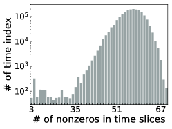
(a) Beijing Air Quality

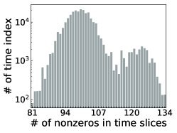
(b) Madrid Air Quality

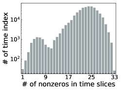
(c) Radar Traffic

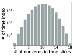
(d) Indoor Condition

(e) Server Room

Figure 3: Time-varying density of five real-world datasets. The horizontal axis represents the unique number of nonzero entries in time slices. The vertical axis represents the number of time indices with such number of nonzeros. Note that time slices have varying densities

We describe how to further improve the accuracy of our method by considering the sparsity of time slices. The loss function (2) uses the same smoothing regularization penalty $\lambda_{t}$ for all the time factor vectors. However, different time slices have different sparsity due to the different number of nonzeros in time slices (see Fig. 3), and it is thus desired to design our method so that it controls the degree of regularization penalty depending on the sparsity. For example, consider the 3-mode air quality tensor $\boldsymbol{\mathscr{X}}$ (time, location, type of pollutants; measurements), introduced in Section 3.2, containing measurements of pollutant at a specific time and location. Assume that the time slice $\boldsymbol{\mathscr{X}}_{t_{1}}$ at time $t_{1}$ is very sparse containing few nonzeros, while the time slice $\boldsymbol{\mathscr{X}}_{t_{2}}$ at time $t_{2}$ is dense with many nonzeros. The factor row $\mathbf{a}_{i_{t_{2}}}^{(1)}$ at time $t_{2}$ can be updated easily using its many nonzeros. However, the factor row $\mathbf{a}_{i_{t_{1}}}^{(1)}$ at time $t_{1}$ does not have enough nonzeros at its corresponding time slice, and thus it is hard to train $\mathbf{a}_{i_{t_{1}}}^{(1)}$ using only its few nonzeros; we need to actively use nearby slices to make up for the lack of data. Thus, it is desired to impose more smoothing regularization at time $t_{1}$ than at time $t_{2}$.

Based on the motivation, TATD controls the degree of smoothing regularization based on the sparsity of time slices. Let the time sparsity $\beta_{i_{t}}$ of the $i_{t}$th time slice be defined as

$$\beta_{i_{t}} =1-d_{i_{t}}$$ (5)

where a time density $d_{i_{t}}$ is defined as follows:

$$d_{i_{t}} =(0.999-0.001)\frac{\omega_{i_{t}}-\omega_{\textit{min}}}{\omega_{\textit{max}}-\omega_{\textit{min}}}+0.001$$ (6)

$\omega_{i_{t}}$ indicates the number of nonzeros at $i_{t}$th time slice; $\omega_{\textit{max}}$ and $\omega_{\textit{min}}$ are the maximum and the minimum values of the number of nonzeros in time slices, respectively. The time density $d_{i_{t}}$ can be thought of as a min-max normalized version of $\omega_{i_{t}}$, with its range regularized to [$0.001$, $0.999$].

Using the defined time sparsity, we modify our objective function as follows.

$$\boldsymbol{\mathscr{L}}=\sum_{\alpha\in\Omega}{\left({x}_{\alpha}-\sum_{k=1}^{K}\prod_{n=1}^{N}a^{(n)}_{i_{n}k}\right)^{2}}+\sum_{i_{t}=1}^{I_{t}}\lambda_{t}\beta_{i_{t}}||{{\mathbf{a}}_{i_{t}}^{(t)}}-{{\tilde{\mathbf{a}}_{i_{t}}^{(t)}}}||_{2}^{2}+\lambda_{r}\sum_{n\neq t}^{N}\lVert{\mathbf{A}^{(n)}}\rVert_{\text{F}}^{2}$$ (7)

Note that the second term is changed to include the time sparsity $\beta_{i_{t}}$; this makes the degree of the regularization vary depending on the sparsity of time slices.

Given the modified objective function in Equation (7), we focus on minimizing the difference between $\mathbf{a}_{i_{t}}^{(t)}$ and $\tilde{\mathbf{a}}_{i_{t}}^{(t)}$ for time slices with a high sparsity rather than those with a low sparsity. TATD actively exploits the neighboring time slices when a target time slice is sparse, while it less exploits the neighboring ones for a dense time slice.

3.4 Optimization

Input :  Tensor $\boldsymbol{\mathscr{X}}\in\mathbf{R}^{I_{1}\times I_{2}\times\cdots\times I_{N}}$ with observed entries $\forall\alpha=(i_{1},\dots,i_{n})\in\Omega$, rank $K$, window size $S$, sparsity penalty $\lambda_{t}$$\beta_{i_{t}}$, regularization parameter $\lambda_{r}$, and learning rate $\eta$

Output :  Updated factor matrices $\mathbf{A}^{(n)}\in{R}^{I_{n}\times k}$ $(n=1...N)$

1 initialize all factor matrices $\mathbf{A}^{(n)}$ for $n=1...N$

2repeat

3       for $n=1...N$ do

4             loss $\boldsymbol{\mathscr{L}}$ $\leftarrow$ Eq. (7)

5             if $n$ is a time mode then

6                   repeat

7                        update a factor $\mathbf{A}^{(n)}$ using Adam optimizer with a learning rate $\eta$

8                  until convergence criterion is met;

9            else

10                   for $i_{n}=1...I_{n}$ do

11                         update a row factor $\mathbf{a}_{i_{n}}^{(n)}$ using the row-wise update rule

12                  

13            

14      

15until convergence criterion is met;

Algorithm 1 Training TATD

To minimize the objective function in Equation (7), TATD uses an alternating optimization method; it updates one factor matrix at a time while fixing all other factor matrices. TATD updates non-time factor matrices using the row-wise update rule (Shin et al. 2016) while updating the time factor matrix using the Adam optimizer (Kingma and Ba 2014). It allows TATD to quickly converge with a low error, compared to naive gradient-based methods.

Updating non-time factor matrix. We note that updating a non-time factor matrix while fixing all other factor matrices is solved via the least square method, and we use the row-wise update rule (Shin et al. 2016; Oh et al. 2018) in ALS for it. The row-wise update rule is advantageous since it gives the optimal closed-form solution, and allows parallel update of factors. We describe the details of the row-wise update rule in Appendix A.1.

Updating time factor matrix. Updating the time factor matrix while fixing all other factor matrices is not the least square problem any more, and thus we turn to gradient based methods. We use the Adam optimizer which has shown superior performance for recent machine learning tasks. We verify that using the Adam optimizer only for the time factor leads to faster convergence compared to other optimization methods in Section 4.

Overall training. Algorithm 1 describes how we train TATD. We first initialize all factor matrices (line 1). For each iteration, we update a factor matrix while keeping all others fixed (lines 1 to 1). The time factor matrix is updated with Adam optimizer (line 1) until the validation RMSE increases, which is our convergence criterion (line 8) for Adam. Each of the non-time factor matrices is updated with the row-wise update rule (line 1) in ALS. We repeat this process until the validation RMSE continuously increases for five iterations, which is our global convergence criterion (line 12).

4 Experiment

We perform experiments to answer the following questions.

• Accuracy (Section 4.2). How accurately does TATD factorize real-world temporal tensors and predict their missing entries compared to other methods?

• Effect of data sparsity (Section 4.3). How does the sparsity of input tensors affect the predictive performance of TATD and other methods?

• Effect of optimization (Section 4.4). How effective is our proposed optimization approach for training TATD?

• Hyper-parameter study (Section 4.5). How do the different hyper-parameter settings affect the performance of TATD?

4.1 Experimental Settings

4.1.1 Machine

All experiments are performed on a machine equipped with Intel Xeon E5-2630 CPU and a Geforce GTX 1080 Ti GPU.

4.1.2 Datasets

Table 2: Summary of real-world tensors used for experiments. Bold text denotes time mode

Name	Dimensionality	Nonzero	Granularity	Density
Beijing Air Quality 1	35,064 $\times$ 12 $\times$ 6	2,454,305	1 hour	0.97
Madrid Air Quality 2	2,678 $\times$ 24 $\times$ 14	337,759	1 day	0.37
Radar Traffic 3	17,937 $\times$ 23 $\times$ 5	495,685	1 hour	0.24
Indoor Condition 4	19,735 $\times$ 9 $\times$ 2	241,201	10 minutes	0.70
Server Room 5	3 $\times$ 3 $\times$ 34 $\times$ 4,157	1,009,426	1 second	0.79

• https://archive.ics.uci.edu/ml/datasets/Beijing+Multi-Site+Air-Quality+Data

• https://www.kaggle.com/decide-soluciones/air-quality-madrid

• https://data.austintexas.gov/Transportation-and-Mobility/Radar-Traffic-Counts/

• https://archive.ics.uci.edu/ml/datasets/Appliances+energy+prediction

• https://zenodo.org/record/3610078#.XlNpAigzaM8

We evaluate TATD on five real-world datasets summarized in Table 2.

• Beijing Air Quality (Zhang et al. 2017) is a 3-mode tensor (hour, locations, atmospheric pollutants) containing measurements of pollutants. It was collected from $12$ air-quality monitoring sites in Beijing between 2013 to 2017.

• Madrid Air Quality is a 3-mode tensor (day, locations, atmospheric pollutants) containing measurements of pollutants in Madrid between 2011 to 2018.

• Radar Traffic is a 3-mode tensor (hour, locations, directions) containing traffic volumes measured by radar sensors from 2017 to 2019 in Austin, Texas.

• Indoor Condition is a 3-mode tensor (10 minutes, locations, ambient conditions) containing measurements. There are two ambient conditions defined: humidity and temperature. We construct a fully dense tensor from the original dataset and randomly sample $70$ percent of the elements to make a tensor with missing entries. In Section 4.3, we sample from the fully dense version of it.

• Server Room is a 4-mode tensor (air conditioning, server power, locations, second) containing temperatures recorded in a server room. The first mode ”air conditioning” means air conditioning temperature setups ($24$, $27$, and $30$ Celsius degrees); the second mode ”server power” indicates server power usage scenarios ($50\%$, $75\%$, and $100\%$).

Before applying tensor factorization, we z-normalize the datasets. Each data is randomly split into training, validation, and test sets with the ratio $8$:$1$:$1$; the validation set is used for determining early stopping.

4.1.3 Competitors

We compare TATD with the state-of-the-art methods for missing entry prediction. All the competitors use only the observed entries of a given tensor.

• CP-ALS (Harshman et al. 1970): a standard CP decomposition method using ALS.

• CP-WOPT (Acar et al. 2011): a CP decomposition method solving a weighted least squares problem.

• CoSTCo (Liu et al. 2019): a CNN-based tensor decomposition method.

• TRMF (Yu et al. 2016): a temporally regularized matrix/tensor factorization method.

• NTF (Wu et al. 2019): a tensor factorization method integrating LSTM to model time-evolving interactions for rating prediction.

4.1.4 Metrics

We evaluate the performance using RMSE (Root Mean Squared Error) and MAE (Mean Absolute Error) defined as follows.

$$\text{RMSE}={\sqrt{\frac{1}{|\Omega|}\sum_{\forall\alpha\in\Omega}{\left(x_{\alpha}-\hat{x}_{\alpha}\right)^{2}}}},\quad\text{MAE}=\frac{1}{|\Omega|}{\sum_{\forall\alpha\in\Omega}{|x_{\alpha}-\hat{x}_{\alpha}|}}$$

$\Omega$ indicates the set of the indices of observed entries. $x_{\alpha}$ stands for the entry with index $\alpha$ and $\hat{x}_{\alpha}$ is the corresponding reconstructed value.

4.1.5 Hyper-parameter

We use hyper-parameters in Table 3 for TATD, except in Section 4.5 where we vary hyper-parameters. We use $0.5$ for $\sigma$ which adjusts the smoothing level in kernel function. We change the window size $S\in\{3,5,7,9,11\}$ and find the optimal value for each dataset.

Table 3: Default hyper-parameter setting

Dataset	Learning rate $\eta$	Rank $K$	Window $S$	Penalty $\lambda_{t}$
Beijing Air Quality	$10^{-2}$	$10$	$3$	$10^{3}$
Madrid Air Quality	$10^{-2}$	$10$	$5$	$10^{2}$
Radar Traffic	$10^{-2}$	$10$	$9$	$10^{2}$
Indoor Condition	$10^{-2}$	$10$	$3$	$10^{2}$
Server Room	$10^{-3}$	$10$	$3$	$10^{-1}$

4.2 Accuracy (Q1)

We compare TATD with competitors in terms of RMSE and MAE in Table 4. TATD-0 indicates TATD without the sparsity penalty. Note that TATD consistently gives the best accuracy for all the datasets. TATD achieves up to $7.01\times$ lower RMSE and $5.50\times$ lower MAE compared to the second-best methods. TATD-0 provides the second-best performance; the smoothing regularization effectively predicts missing values by capturing temporal patterns and leaving out the noise.

Table 4: Performance of missing entry prediction by TATD and competitors. The best method is in bold, and the second-best method is underlined. Our proposed TATD consistently shows the best performance in all datasets

Data	Beijing Air quality	Madrid Air quality	Radar Traffic	Indoor Condition	Server Room
	RMSE / MAE	RMSE / MAE	RMSE / MAE	RMSE / MAE	RMSE / MAE
CP-ALS	0.352 / 0.219	0.456 / 0.293	0.365 / 0.248	0.624 / 0.316	0.076 / 0.048
CP-WOPT	0.766 / 0.538	0.482 / 0.297	0.328 / 0.206	0.603 / 0.310	0.070 / 0.046
CoSTCo	0.360 / 0.223	0.461 / 0.303	0.298 / 0.197	0.609 / 0.303	0.306 / 0.090
TRMF	1.098 / 0.770	1.004 / 0.936	0.695 / 0.485	0.894 / 0.563	1.083 / 0.813
NTF	0.529 / 0.333	0.648 / 0.455	0.585 / 0.400	0.968 / 0.576	0.660 / 0.516
TATD-0	0.327 / 0.204	0.416 / 0.279	0.257 / 0.160	0.088 / 0.057	0.058 / 0.039
TATD (proposed)	0.323 / 0.201	0.409 / 0.274	0.249 / 0.152	0.086 / 0.055	0.054 / 0.035

4.3 Effect of Data Sparsity (Q2)

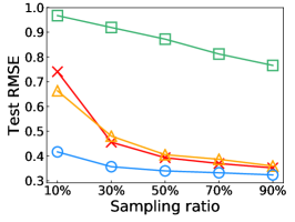
(a) Beijing Air Quality

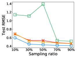
(b) Madrid Air Quality

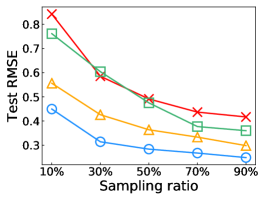
(c) Radar Traffic

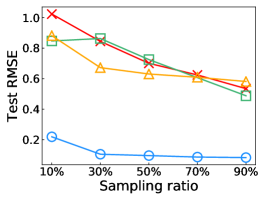
(d) Indoor Condition

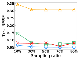
(e) Server Room

Figure 4: Test RMSE of TATD and the best competitors CP-ALS, CP-WOPT and CoSTCo for varying data sampling ratio. Note that the error gap of TATD and competitors becomes larger when the sparsity increases (the sampling ratio decreases), due to the careful consideration of sparse time slices by TATD.

We evaluate the performance of TATD with varying data sparsity. We sample the data with the ratio of $\{10,30,50,70,90\}\%$ to identify how accurately the method predicts missing entries even when the data are highly sparse. Fig. 4 shows the errors of TATD and the best competitors, CP-ALS, CP-WOPT, and CoSTCo, for five datasets. Note that the error gap of TATD and competitors becomes larger when the sparsity increases (the sampling ratio decreases). TATD achieves up to $4.67\times$, $3.86\times$ and $5.24\times$ lower test RMSE than CP-ALS, CP-WOPT, and CoSTCo, respectively, when we use only $10\%$ of data. There are two reasons for the superior performance of TATD as the sparsity increases. First, TATD is designed to infer missing entries of a target slice by using its neighboring slices; this is especially useful when the target slice is extremely sparse and has no information to infer its entries. Second, TATD explicitly considers sparsity in its model through the sparsity penalty, and imposes more regularization for sparser slices.

4.4 Effect of Optimization (Q3)

We evaluate our optimization strategy in terms of error and running time. We call our strategy as ALS + Adam and compare it with the following optimization strategies.

• Adam: a recent gradient-based method using momentum and controlling learning rate.

• SGD: a standard stochastic gradient descent method which is widely used for optimization.

• ALS + SGD: an alternating minimization method which updates a time factor matrix with SGD and non-time factor matrices with the least square solution.

• Alternating Adam: an alternating minimization method which updates a single factor matrix with Adam while fixing other factor matrices.

Fig. 5 shows the result. Note that our proposed ALS + Adam makes the best trade-off of running time and test RMSE, giving smaller running time and test RMSE compared to other methods in general. ALS + Adam achieves better results compared to ALS + SGD since Adam optimizer finds a better local minimum compared to SGD. Compared to alternating Adam, ALS + Adam achieves better results as well since updating each non-time factor matrix has an analytical solution by ALS, and thus a gradient-based approach Adam is less effective.

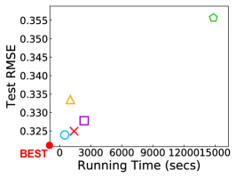
(a) Beijing Air Quality

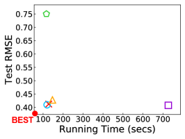
(b) Madrid Air Quality

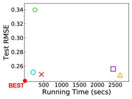
(c) Radar Traffic

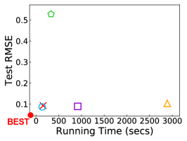
(d) Indoor Condition

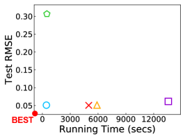
(e) Server Room

Figure 5: Comparison of optimization strategies in TATD. Our proposed ALS + Adam makes the best trade-off of running time and test RMSE, giving smaller running time and test RMSE compared to other methods in general

4.5 Hyper-parameter Study (Q4)

We evaluate the performance of TATD with regard to hyper-parameters: smoothing regularization penalty and rank size.

4.5.1 Smoothing regularization penalty

We vary the smoothing regularization penalty $\lambda_{t}$ and evaluate the test RMSE in Fig. 6. Note that too small or too large values of $\lambda_{t}$ do not give the best results; too small value of $\lambda_{t}$ leads to overfitting, and too large value of it leads to underfitting. The results show that a right amount of smoothing regularization gives the smallest error, verifying the effectiveness of our proposed idea.

4.5.2 Rank

We increase the rank $K$ from $5$ to $50$ and evaluate the test RMSE in Fig. 7. We have two main observations. First, TATD shows a stable performance improvement with increasing ranks, compared to CP-ALS and CP-WOPT which show unstable performances. Second, the error gap between TATD and competitors increases with increasing ranks. Higher ranks may make the models overfit to a training dataset; however, TATD works even better for higher ranks since it exploits rich information from neighboring rows when regularizing a row of the time factor matrix.

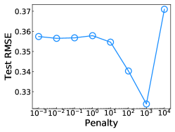
(a) Beijing Air Quality

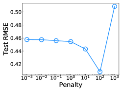
(b) Madrid Air Quality

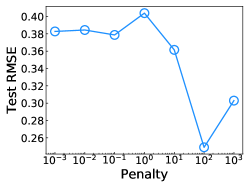
(c) Radar Traffic

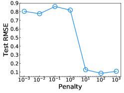
(d) Indoor Condition

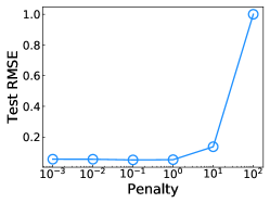
(e) Server Room

Figure 6: Effect of the smoothing regularization penalty parameter $\lambda_{t}$ in TATD. Note that too small or too large values of $\lambda_{t}$ lead to overfitting and underfitting, respectively. A right amount of smoothing regularization gives the smallest error, verifying the effectiveness of our proposed idea

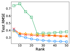
(a) Beijing Air Quality

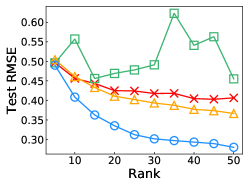
(b) Madrid Air Quality

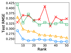
(c) Radar Traffic

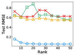
(d) Indoor Condition

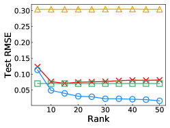
(e) Server Room

Figure 7: Effect of rank on the performance of TATD. When the rank increase, TATD shows a stable performance improvement unlike competitors, and the error gap between TATD and competitors increases. TATD works even better for higher ranks since it exploits rich information from neighboring rows when regularizing a row of the time factor matrix.

5 Related Work

We describe related works on tensor factorization and missing entry prediction on temporal tensors.

5.1 Tensor Decomposition

We present one of the major tensor decomposition methods, CP decomposition.

CP decomposition. CP decomposition methods (Kang et al. 2012; Jeon et al. 2015; Choi and Vishwanathan 2014) have been widely used for analyzing large-scale real-world tensors. Kang et al. (2012); Jeon et al. (2015) propose distributed CP decomposition methods running on the MapReduce framework. Choi and Vishwanathan (2014) propose a scalable CP decomposition method by exploiting properties of a tensor operation used in CP decomposition. Battaglino et al. (2018) propose a randomized CP decomposition method which reduces the overhead of computation and memory. However, the above methods are not appropriate for missing value prediction in highly sparse tensors since they assume the values of missing entries are zero.

Several CP decomposition methods have been developed to handle sparse tensors without setting the values of missing entries as zero. Papalexakis et al. (2012) propose ParCube to obtain sparse factor matrices using a sampling technique in parallel systems. Beutel et al. (2014) propose FlexiFaCT, which performs a coupled matrix-tensor factorization using Stochastic Gradient Descent (SGD) update rules. Shin et al. (2016) propose CDTF and SALS, which are scalable CP decomposition methods for sparse tensors. Smith and Karypis (2017) improves the efficiency of CP decomposition for sparse tensors by exploiting a compressed data structure. The above CP decomposition methods do not consider temporal dependency and time-varying sparsity which are crucial for temporal tensors. On the other hand, TATD improves accuracy for temporal tensors by exploiting temporal dependency and time-varying sparsity.

Applications. Tensor decomposition have been used for various applications. Kolda et al. (2005) analyze a hyperlink graph modeled as $3$-way tensor using CP decomposition. Tensor decomposition is also applied to tag recommendation (Rendle et al. 2009; Rendle and Schmidt-Thieme 2010). Sun et al. (2009) develop a content-based network analysis framework for finding higher-order clusters. Lebedev et al. (2015) exploit CP decomposition to compress convolution filters of convolutional neural networks (CNNs). Several works (Lee et al. 2018; Perros et al. 2017, 2018) use tensor decomposition for analyzing Electronic Health Record (EHR) data.

5.2 Tensor Factorization on Temporal Tensors

We explain tensor factorization methods dealing with temporal data. Dunlavy et al. (2011) propose a tensor-based approach with an exponential smoothing technique for link prediction. Matsubara et al. (2012) discover main topics in a complex temporal tensor and perform analysis for long periods of prediction. de Araujo et al. (2017) present a non-negative coupled tensor factorization for forecasting future links in evolving networks. Bahadori et al. (2014) propose an efficient low-rank tensor method to capture shared structures across multivariate spatial-temporal relationships. Liu et al. (2019) propose a tensor completion method by exploiting the expressive power of convolutional neural networks to model non-linear interactions inside spatio-temporal tensors. These works focus on general multi faceted relationships rather than temporal characteristics.

Several works (Xiong et al. 2010; Yu et al. 2016; Wu et al. 2019) model temporal patterns and trends in temporal tensors. Xiong et al. (2010) propose a Bayesian probabilistic tensor factorization method that learns global temporal patterns by adding an extra time factor to model evolving relations in a matrix. Yu et al. (2016) propose a matrix factorization method with an autoregressive temporal regularization to learn a temporal property. Wu et al. (2019) propose a CP factorization method based on a long short-term memory network to model temporal interactions between latent factors of tensors. Jing et al. (2018) propose a tucker decomposition method to capture temporal correlations. However, these approaches are not designed for modeling temporal dependency from both past and future information, whereas TATD obtains a time factor considering neighboring factors for both past and future time steps, giving an accurate tensor factorization result. Moreover, they do not exploit the temporal sparsity, a common characteristic of a temporal tensor, while TATD actively exploits the temporal sparsity.

6 Conclusion

We propose TATD (Time-Aware Tensor Decomposition), a novel tensor factorization method for temporal tensors to accurately predict missing entries. To capture temporal dependency and sparsity in real world temporal tensors, we design a smoothing regularization on time factor, and adjust the amount of the regularization according to the sparsity of time slices. Moreover, we accurately and efficiently optimize TATD with a carefully designed optimization strategy. Extensive experimental results show that TATD achieves up to $7.01\times$ lower RMSE and $5.50\times$ lower MAE compared to the second best methods. Future works include extending TATD for an online or a distributed setting.

Appendix A Appendix

A.1 Row-wise Update Rule

We use a row-wise update rule to efficiently update non-time factor matrices. This update rule has an advantage of considering only nonzero values and allows easy parallelization. Following the notations and equations introduced by Shin et al. (2016), the update rule for $i_{n}$th row of the $n$th factor matrix $\mathbf{A}^{(n)}(n\neq t)$ is given as follows:

$$\begin{split}[a_{i_{n}1}^{(n)},\cdots,a_{i_{n}K}^{(n)}]\leftarrow\underset{[a^{(n)}_{i_{n}1},...,a^{(n)}_{i_{n}K}]}{\operatorname{arg}\,\operatorname{min}}\;{L(\mathbf{A}^{(1)},...,\mathbf{A}^{(N)})}\\ =\mathbf{c}_{i_{n}:}^{(n)}\times[\mathbf{B}_{i_{n}}^{(n)}+\lambda_{r}\mathbf{I}_{K}]^{-1}\text{ }\end{split}$$ (8)

where $\mathbf{B}_{i_{n}}^{(n)}$ is a ${K\times K}$ matrix whose entries are

$${(\mathbf{B}_{i_{n}}^{(n)})}_{k_{1}k_{2}}=\sum_{\forall\alpha\in\Omega_{i_{n}}^{(n)}}\prod_{l\neq n}a^{(l)}_{i_{l}k_{1}}\prod_{l\neq n}a^{(l)}_{i_{l}k_{2}},\forall k_{1},k_{2}$$ (9)

, $\mathbf{c}_{i_{n}}^{(n)}$ is a length ${K}$ vector whose entries are

$$\sum_{\forall\alpha\in\Omega_{i_{n}}^{(n)}}x_{\alpha}\prod_{l\neq n}a^{(l)}_{i_{l}k},\forall k$$ (10)

and $\Omega_{i_{n}}^{(n)}$ denotes the subset of $\Omega$ whose $n$th mode’s index is $i_{n}$.

References

- Acar et al. (2011) Acar E, Dunlavy DM, Kolda TG, Mørup M (2011) Scalable tensor factorizations for incomplete data. Chemometrics and Intelligent Laboratory Systems 106(1):41–56
- Ahn et al. (2020) Ahn D, Son S, Kang U (2020) Gtensor: Fast and accurate tensor analysis system using gpus. In: Proceedings of the 29th ACM International Conference on Information and Knowledge Management, CIKM 2020, October 19-23, 2020
- de Araujo et al. (2017) de Araujo MR, Ribeiro PMP, Faloutsos C (2017) Tensorcast: Forecasting with context using coupled tensors (best paper award). In: 2017 IEEE International Conference on Data Mining (ICDM), IEEE, pp 71–80
- Bahadori et al. (2014) Bahadori MT, Yu QR, Liu Y (2014) Fast multivariate spatio-temporal analysis via low rank tensor learning. In: Advances in neural information processing systems, pp 3491–3499
- Battaglino et al. (2018) Battaglino C, Ballard G, Kolda TG (2018) A practical randomized CP tensor decomposition. SIAM J Matrix Analysis Applications 39(2):876–901
- Beutel et al. (2014) Beutel A, Talukdar PP, Kumar A, Faloutsos C, Papalexakis EE, Xing EP (2014) Flexifact: Scalable flexible factorization of coupled tensors on hadoop. In: Proceedings of the 2014 SIAM International Conference on Data Mining, Philadelphia, Pennsylvania, USA, April 24-26, 2014, SIAM, pp 109–117
- Choi et al. (2019) Choi D, Jang JG, Kang U (2019) S3cmtf: Fast, accurate, and scalable method for incomplete coupled matrix-tensor factorization. PLOS ONE 14(6):1–20
- Choi and Vishwanathan (2014) Choi JH, Vishwanathan S (2014) Dfacto: Distributed factorization of tensors. In: Ghahramani Z, Welling M, Cortes C, Lawrence ND, Weinberger KQ (eds) Advances in Neural Information Processing Systems 27: Annual Conference on Neural Information Processing Systems 2014, December 8-13 2014, Montreal, Quebec, Canada, pp 1296–1304
- Dunlavy et al. (2011) Dunlavy DM, Kolda TG, Acar E (2011) Temporal link prediction using matrix and tensor factorizations. ACM Transactions on Knowledge Discovery from Data (TKDD) 5(2):10
- Harshman et al. (1970) Harshman RA, et al. (1970) Foundations of the parafac procedure: Models and conditions for an” explanatory” multimodal factor analysis
- Jeon et al. (2016a) Jeon B, Jeon I, Sael L, Kang U (2016a) Scout: Scalable coupled matrix-tensor factorization - algorithm and discoveries. In: 32nd IEEE International Conference on Data Engineering, ICDE 2016, Helsinki, Finland, May 16-20, 2016, pp 811–822
- Jeon et al. (2015) Jeon I, Papalexakis EE, Kang U, Faloutsos C (2015) Haten2: Billion-scale tensor decompositions. In: 2015 IEEE 31st International Conference on Data Engineering, IEEE, pp 1047–1058
- Jeon et al. (2016b) Jeon I, Papalexakis EE, Faloutsos C, Sael L, Kang U (2016b) Mining billion-scale tensors: algorithms and discoveries. VLDB J 25(4):519–544
- Jing et al. (2018) Jing P, Su Y, Jin X, Zhang C (2018) High-order temporal correlation model learning for time-series prediction. IEEE transactions on cybernetics 49(6):2385–2397
- Kang et al. (2012) Kang U, Papalexakis EE, Harpale A, Faloutsos C (2012) Gigatensor: scaling tensor analysis up by 100 times - algorithms and discoveries. In: KDD, pp 316–324
- Kiers (2000) Kiers HA (2000) Towards a standardized notation and terminology in multiway analysis. Journal of Chemometrics: A Journal of the Chemometrics Society 14(3):105–122
- Kingma and Ba (2014) Kingma DP, Ba J (2014) Adam: A method for stochastic optimization. arXiv preprint arXiv:14126980
- Kolda and Sun (2008) Kolda TG, Sun J (2008) Scalable tensor decompositions for multi-aspect data mining. In: 2008 Eighth IEEE international conference on data mining, IEEE, pp 363–372
- Kolda et al. (2005) Kolda TG, Bader BW, Kenny JP (2005) Higher-order web link analysis using multilinear algebra. In: Proceedings of the 5th IEEE International Conference on Data Mining (ICDM 2005), 27-30 November 2005, Houston, Texas, USA, IEEE Computer Society, pp 242–249
- Lebedev et al. (2015) Lebedev V, Ganin Y, Rakhuba M, Oseledets IV, Lempitsky VS (2015) Speeding-up convolutional neural networks using fine-tuned cp-decomposition. In: Bengio Y, LeCun Y (eds) 3rd International Conference on Learning Representations, ICLR 2015, San Diego, CA, USA, May 7-9, 2015, Conference Track Proceedings
- Lee et al. (2018) Lee J, Oh S, Sael L (2018) GIFT: guided and interpretable factorization for tensors with an application to large-scale multi-platform cancer analysis. Bioinform 34(24):4151–4158
- Liu et al. (2019) Liu H, Li Y, Tsang M, Liu Y (2019) Costco: A neural tensor completion model for sparse tensors. Training 10(4):10–3
- Maruhashi et al. (2011) Maruhashi K, Guo F, Faloutsos C (2011) Multiaspectforensics: Pattern mining on large-scale heterogeneous networks with tensor analysis. In: 2011 International Conference on Advances in Social Networks Analysis and Mining, IEEE, pp 203–210
- Matsubara et al. (2012) Matsubara Y, Sakurai Y, Faloutsos C, Iwata T, Yoshikawa M (2012) Fast mining and forecasting of complex time-stamped events. In: Proceedings of the 18th ACM SIGKDD international conference on Knowledge discovery and data mining, ACM, pp 271–279
- Oh et al. (2018) Oh S, Park N, Sael L, Kang U (2018) Scalable tucker factorization for sparse tensors - algorithms and discoveries. In: 34th IEEE International Conference on Data Engineering, ICDE 2018, Paris, France, April 16-19, 2018
- Oh et al. (2019) Oh S, Park N, Jang J, Sael L, Kang U (2019) High-performance tucker factorization on heterogeneous platforms. IEEE Trans Parallel Distrib Syst 30(10):2237–2248
- Papalexakis et al. (2012) Papalexakis EE, Faloutsos C, Sidiropoulos ND (2012) Parcube: Sparse parallelizable tensor decompositions. In: ECML-PKDD, Springer, Lecture Notes in Computer Science, vol 7523, pp 521–536
- Park et al. (2016) Park N, Jeon B, Lee J, Kang U (2016) Bigtensor: Mining billion-scale tensor made easy. In: Proceedings of the 25th ACM International Conference on Information and Knowledge Management, CIKM 2016, Indianapolis, IN, USA, October 24-28, 2016, pp 2457–2460
- Park et al. (2017) Park N, Oh S, Kang U (2017) Fast and scalable distributed boolean tensor factorization. In: 33rd IEEE International Conference on Data Engineering, ICDE 2017, San Diego, CA, USA, April 19-22, 2017, pp 1071–1082
- Park et al. (2019) Park N, Oh S, Kang U (2019) Fast and scalable method for distributed boolean tensor factorization. The VLDB Journal
- Perros et al. (2017) Perros I, Papalexakis EE, Wang F, Vuduc RW, Searles E, Thompson M, Sun J (2017) Spartan: Scalable PARAFAC2 for large & sparse data. In: Proceedings of the 23rd ACM SIGKDD International Conference on Knowledge Discovery and Data Mining, Halifax, NS, Canada, August 13 - 17, 2017, ACM, pp 375–384
- Perros et al. (2018) Perros I, Papalexakis EE, Park H, Vuduc RW, Yan X, deFilippi C, Stewart WF, Sun J (2018) Sustain: Scalable unsupervised scoring for tensors and its application to phenotyping. In: Guo Y, Farooq F (eds) Proceedings of the 24th ACM SIGKDD International Conference on Knowledge Discovery & Data Mining, KDD 2018, London, UK, August 19-23, 2018, ACM, pp 2080–2089
- Rendle and Schmidt-Thieme (2010) Rendle S, Schmidt-Thieme L (2010) Pairwise interaction tensor factorization for personalized tag recommendation. In: WSDM, pp 81–90
- Rendle et al. (2009) Rendle S, Marinho LB, Nanopoulos A, Schmidt-Thieme L (2009) Learning optimal ranking with tensor factorization for tag recommendation. In: SIGKDD, pp 727–736
- Shin and Kang (2014) Shin K, Kang U (2014) Distributed methods for high-dimensional and large-scale tensor factorization. In: 2014 IEEE International Conference on Data Mining, ICDM 2014, Shenzhen, China, December 14-17, 2014, pp 989–994
- Shin et al. (2016) Shin K, Sael L, Kang U (2016) Fully scalable methods for distributed tensor factorization. IEEE Transactions on Knowledge and Data Engineering 29(1):100–113
- Smith and Karypis (2017) Smith S, Karypis G (2017) Accelerating the tucker decomposition with compressed sparse tensors. In: Rivera FF, Pena TF, Cabaleiro JC (eds) Euro-Par 2017: Parallel Processing - 23rd International Conference on Parallel and Distributed Computing, Santiago de Compostela, Spain, August 28 - September 1, 2017, Proceedings, Springer, Lecture Notes in Computer Science, vol 10417, pp 653–668
- Sun et al. (2006) Sun J, Papadimitriou S, Philip SY (2006) Window-based tensor analysis on high-dimensional and multi-aspect streams. In: Sixth International Conference on Data Mining (ICDM’06), IEEE, pp 1076–1080
- Sun et al. (2009) Sun J, Papadimitriou S, Lin C, Cao N, Liu S, Qian W (2009) Multivis: Content-based social network exploration through multi-way visual analysis. In: Proceedings of the SIAM International Conference on Data Mining, SDM 2009, April 30 - May 2, 2009, Sparks, Nevada, USA, SIAM, pp 1064–1075
- Sun et al. (2015) Sun Y, Gao J, Hong X, Mishra B, Yin B (2015) Heterogeneous tensor decomposition for clustering via manifold optimization. IEEE transactions on pattern analysis and machine intelligence 38(3):476–489
- Symeonidis (2016) Symeonidis P (2016) Matrix and tensor decomposition in recommender systems. In: Proceedings of the 10th ACM Conference on Recommender Systems, pp 429–430
- Wu et al. (2019) Wu X, Shi B, Dong Y, Huang C, Chawla NV (2019) Neural tensor factorization for temporal interaction learning. In: Proceedings of the Twelfth ACM International Conference on Web Search and Data Mining, pp 537–545
- Xiong et al. (2010) Xiong L, Chen X, Huang TK, Schneider J, Carbonell JG (2010) Temporal collaborative filtering with bayesian probabilistic tensor factorization. In: Proceedings of the 2010 SIAM International Conference on Data Mining, SIAM, pp 211–222
- Yu et al. (2016) Yu HF, Rao N, Dhillon IS (2016) Temporal regularized matrix factorization for high-dimensional time series prediction. In: Advances in neural information processing systems, pp 847–855
- Zhang et al. (2017) Zhang S, Guo B, Dong A, He J, Xu Z, Chen SX (2017) Cautionary tales on air-quality improvement in beijing. Proceedings of the Royal Society A: Mathematical, Physical and Engineering Sciences 473(2205):20170457