Non-Sinusoidal Transit Timing Variations for the Exoplanet HAT-P-12b

Abstract

Considering the importance of investigating the transit timing variations (TTVs) of transiting exoplanets, we present a follow-up study of HAT-P-12b. We include six new light curves observed between 2011 and 2015 from three different observatories, in association with 25 light curves taken from the published literature. The sample of the data used, thus covers a time span of $\sim 10.2$ years with a large coverage of epochs (1160) for the transiting events of the exoplanet HAT-P-12b. The light curves are used to determine the orbital parameters and conduct an investigation of possible transit timing variations. The new linear ephemeris shows a large value of reduced $\chi^{2}$, i.e. $\chi^{2}_{red}(23)$ = 7.93, and the sinusoidal fitting using the prominent frequency coming from a periodogram shows a reduced $\chi^{2}$ around 4. Based on these values and the corresponding $O-C$ diagrams, we suspect the presence of a possible non-sinusoidal TTV in this planetary system. Finally, we find that a scenario with an additional non-transiting exoplanet could explain this TTV with an even smaller reduced $\chi^{2}$ value of around 2.

1 Introduction

Many generations of astronomers have been seraching for the possible existence of exoplanets before the end of twentieth century (Briot & Schneider 2018) with the discovery of 51 Peg b (Mayor & Queloz 1995). Since then, exoplanetary science has witnessed a boom that has made it one of the most studied branches of astronomy. Although the initial success in discovering exoplanets came from the results of the Doppler method, the transit method has played the most dominating role in discovering new exoplanets. This is due to space-based surveys like Kepler (Borucki et al 2010), K2 (Howell et al. 2014), Convection, Rotation and planetary Transits (CoRoT, Baglin et al. 2006) and also, the recently launched Transiting Exoplanet Survey Satellite (TESS, Ricker et al. 2015). However, transit surveys from ground-based observing facilities have also contributed significantly in discovering transiting exoplanets owing to the surveys such as the Hungarian-made Automated Telescope Network (HATNet, Bakos et al. 2004), The Hungarian-made Automated Telescope Network-South (HATSouth, Bakos et al. 2013), Trans-Atlantic Exoplanet Survey (TrES, Alonso et al. 2004), Super Wide Angle Search for Planets (SuperWASP, Pollacco et al. 2006), Kilodegree Extremely Little Telescope (KELT, Pepper et al. 2007), Qatar Exoplanet Survey (QES, Alsubai et al. 2013), Multi-site All-Sky CAmeRA (MASCARA, Talens et al. 2017) survey to name a few. These surveys preferably detect short period, close-in planets. Ground-based telescopes also provide follow-up observations to confirm the transiting nature of exoplanets discovered from space surveys.

The additional contributions from ground-based telescopes are to cover a large field-of-view and to carry out extensive follow-up observation programs which improve the orbital parameters of a planetary system. These observations can also be used for the analysis of the transit timing variations (TTVs) over a longer time baseline. In essence, a TTV is the transit time deviation from a linear ephemeris which provides clues about the existence of another planet in the system (Agol et al. 2005, Agol & Fabrycky 2017, Sun et al. 2017, Linial et al. 2018, Baştürk et al. 2019). In fact, TTVs have not only led to the discoveries of new exoplanets (Nesvorný et al. 2012, Ioannidis et al. 2014, Fox & Wiegert 2019, Sun et al. 2019), but also become a tool to characterize the bulk composition of exoplanets (Jontof-Hutter et al. 2015, Kipping et al. 2019). Motivated by these important results, Holczer et al. (2016) constructed a transit timing catalog of 2599 Kepler Objects of Interest, which will be very useful for further TTV studies.

As discussed by Baştürk et al. (2019), Saturn mass planets are interesting for their densities and orbital properties. HAT-P-12b is a low-density, moderately irradiated, sub-Saturn mass ($m_{p}=0.211\pm 0.012M_{J}$) transiting exoplanet whose discovery was reported by Hartman et al. (2009) using the HAT-5 telescope (located in Arizona) of HATNet (Bakos et al. 2004). HAT-P-12b orbits a moderately bright ($V\sim 12.8$), metal-poor K4 dwarf within a period of $\sim$3.21 days (Hartman et al. 2009). By the time of its discovery, it was the least massive H/He-dominated gas giant planet. Because the above characteristics are very different from Jupiter-mass close-in exoplanets, HAT-P-12b has been studied through the methods of photometric transit observations, radial velocity measurements, and transmission spectroscopy by many groups. Lee et al. (2012) used follow-up observations to improve the ephemeris of the system. Likewise, Sada et al. (2012) published $J$-band transit light curves for HAT-P-12b. Todorov et al. (2013) observed the secondary eclipses using the IRAC instrument on the Spitzer Space Telescope. They did not detect eclipses at either 4.5 $\mu$m or 3.6 $\mu$m wavelengths. The radial velocity measurements of the planet were produced by Kunston et al. (2014) and Ment et al. (2018). Mancini et al. (2018) used HARPS-N high-precision radial velocity measurements to analyze the Rossiter-McLaughlin effect. They determined the sky-projected obliquity ($\lambda=-54^{\circ}\,{}^{+41^{\circ}}_{-13^{\circ}}$) for HAT-P-12b. Sada & Ramon-Fox (2016) combined publicly available light curves with radial velocity measurements and determine physical and orbital parameters for HAT-P-12b. Spectroscopically, Line et al. (2013) presented an NIR transmission spectrum for the system using HST WFC-3. They found a lack of water absorption feature for a hydrogen-dominated atmosphere. Alexoudi et al. (2018) performed a homogeneous analysis which included published data from Sing et al. (2016) and their own data and obtained a transmission spectrum with a low-amplitude spectral slope.

The above discussion shows that the determination of updated orbital parameters is very important as small deviations in these values could lead to different physical parameters and structures of exoplanets. Motivated by this, through a homogeneous long baseline TTV analysis, here we present a comprehensive study of HAT-P-12b with observations combining our new observations with the publicly available published light curves. We include the light curves from the discovery paper of HAT-P-12b (Hartman et al. 2009), up to very recent observations, in order to cover a large range of 1160 epochs, where the entire data has a time baseline of $\sim 10.2$ years.

The data used in this work and its basic reduction procedure are given in Section 2. The analysis of the light curves using Markov-Chain Monte-Carlo (MCMC) techniques is described in Section 3. Section 4 describes a new ephemeris using linear fitting as well as a frequency analysis and corresponding $O-C$ diagrams. Section 5 presents the dynamical two-planet model. Finally, the conclusions of this study are presented in Section 6.

2 The Data and Reduction Procedures

Table 1: The observational log of the new data used in this work.

Run	UT Date	Instrument	Filter	Interval	Exposure	Number of
				($BJD_{TDB}-2450000$)	(s)	images
1	2011 March 29	Tenagra	$R$	5649.712644-5649.930803	75	192
2	2011 April 17	PM0	Sloan $r$	5668.988182-5669.165950	50	159
3	2011 April 27	Tenagra	$R$	5678.633962-5678.848666	75	144
4	2014 March 19	P60	$R$	6735.744668-6735.888703	15	276
5	2014 April 17	P60	$R$	6764.676953-6764.805016	20	216
6	2015 July 14	P60	$R$	7217.695978-7217.850202	24	186

Among our data, we used three transit observations from the 60 inch telescope (P60) installed at the Palomar Observatory in California, USA. Two light curves were observed with 32 inch telescope at Tenagra Observatory in Arizona, USA. The Purple Mountain Observatory’s 40 inch Near-Earth Object Survey Telescope at the Xuyi Station provided another light curve’s data used in this study. The log of the observations is listed in Table LABEL:log. The ‘run’ in the table is in accordance to the date of observation.

The observed CCD images first went through some standard procedures such as bias subtraction, flat-fielding, dark frames (when needed) and cosmic rays removal with Image Reduction and Analysis Facility (IRAF). Before conducting photometry of the images, the images were first aligned using the ‘xregister’ task of IRAF. The photometry of the ‘cleaned’ images is conducted using the ‘apphot’ task in the ‘digiphot’ routine. The initial step in aperture photometry is to find/detect the stars in the image. IRAF task ‘daofind’ finds stars in the image and lists them in a file. The next step in aperture photometry gives the flux value of the stars. IRAF task ‘phot’ serves this purpose.

Once we have the fluxes of stars, we conduct differential photometry. In differential photometry, the target star’s flux (or magnitude) is presented with respect to one or multiple comparison stars (e.g. Sariya et al. 2013, Jiang et al. 2013, 2016). The selected comparison stars should not be of a variable nature. Differential photometry cancels out the corrections required for the airmass and exposure time. It is also useful when the observing conditions are not the best. For the HAT-P-12b data, we selected the comparison stars having the same instrumental magnitude and neighboring position to the target star (HAT-P-12) in the CCD frames.

For the TTV analysis, it is always best to include the published light curves with the new observations as a longer time baseline assures a better ephemeris. We have, therefore, used three light curves from Hartman et al. (2009), three light curves from Lee et al. (2012), ten light curves from Mancini et al. (2018) and nine light curves from Alexoudi et al. (2018). The total time duration covered by the data thus becomes slightly more than a decade.

We did not simply use the mid-transit times for the published light curves given in the respective papers. Instead, we applied the same procedure on those light curves that we applied to our data. This approach removes any systematics while performing parameter fitting and provides more consistent inputs for the TTV analysis.

The light curves were then processed through a normalization routine to get rid of the effects caused by the airmass. For this purpose, we adopted the procedure described by Murgas et al. (2014) wherein a third degree polynomial is used to model the airmass. The observed flux of a light curve $F_{0}(t)$ can be represented as:

$$F_{0}(t)=F(t)\mathcal{P}(t),$$ (1)

where $F(t)$ is the normalized flux of the light curve which will be used in the further analysis and $\mathcal{P}(t)=a_{0}+a_{1}t+a_{2}t^{2}+a_{3}t^{3}$ is a third degree polynomial. A python code is used to numerically calculate the best values of the parameters $a_{0}$, $a_{1}$, $a_{2}$, and $a_{3}$ so that the out-of-transit part of $F(t)$ is close to unity.

As for the timing scheme for the light curves, we took the time from the headers of the individual images. To make sure that the criterion used for the time is uniform, first we calculated observation time for the mid-exposure for every image. Further, it is essential to bring all the mid-exposure times to a common time stamp for a consistent fitting. Hence, all the individual times of observations were converted to the Barycentric Julian Date in Barycentric Dynamical Time (BJD_TDB) following Eastman et al. (2010).

3 The Light-Curve Analysis

Table 2: The settings of initial values and conditions for running the TAP. The values of $P$, $i$, $a/{R_{*}}$ and $R_{p}/R_{*}$ are taken from Hartman et al. (2009). The value of eccentricity ($e$) is taken from Knutson et al. (2014).

Parameter	Initial Value	Condition during MCMC Chains
period ($P$,day)	3.2130598	Gaussian penalty with $\sigma=0.0000021$
orbital inclination ($i$, ∘)	89.0	Gaussian penalty with $\sigma=0.4$
scaled semi-major axis ($a/R_{*}$)	11.77	free
planet to star radius ratio ($R_{p}/R_{*}$)	0.1406	free
mid-transit time ($T_{m}$)	TAP calculations	free, linked only for the same transit event
linear limb darkening ($u_{1}$)	Table LABEL:LD	Gaussian penalty with $\sigma=0.05$
quadratic limb darkening ($u_{2}$)	Table LABEL:LD	Gaussian penalty with $\sigma=0.05$
orbital eccentricity ($e$)	0.026	Gaussian penalty with $\sigma=0.022$
longitude of periastron ($\varpi,^{\circ}$)	0.0	locked

The transit light curves (6 new+25 published) were analyzed using the Transit Analysis Package (TAP, Gazak et al. 2012). TAP has previously been used by our group for TrES-3b (Jiang et al. 2013, Mannaday et al. (2020), WASP-43b (Jiang et al. 2016) and Qatar-1b (Su et al., submitted). TAP is an IDL based graphical user-interface driven software package which employs the MCMC approach to fit the light curves using the analytic model given by Mandel & Agol (2002) and wavelet-based likelihood function by Carter & Winn (2009).

TAP involves a set of nine parameters that the user has to input. These parameters are: orbital period of the planet ($P$), orbital inclination on the sky plane ($i$), scaled semi-major axis ($a/R_{\ast}$), the planet-to-star radius ratio ($R_{\rm p}/R_{\ast}$), the mid-transit time ($T_{\rm m}$), the linear limb darkening coefficient ($u_{1}$), the quadratic limb darkening coefficient ($u_{2}$), orbital eccentricity ($e$) and the longitude of periastron ($\varpi$). For the input parameters mentioned above, one has to define one of the three conditions while running the MCMC chain of TAP. According to the conditions, a parameter can be one of the following: (1) completely free (2) completely locked, or (3) varying according to a Gaussian function.

As discussed in Section 2, we dropped the first publicly available light curve from Hartman et al. (2009). So, the epoch zero in this study was defined by the second of the four publicly available light curves from Hartman et al. (2009). In order to define the initial input values, we considered most of the values mentioned in Hartman et al. (2009), as their paper presents the maximum number of required input parameters and it is better for the consistency to use input parameters from the same source. For the eccentricity, we considered the initial input value from Knutson et al. (2014). The orbital period ($P$) was defined as 3.2130598 with a Gaussian penalty of 0.0000021. The scaled semi-major axis ($a/R_{\ast}$) and the planet-to-star radius ratio ($R_{\rm p}/R_{\ast}$) were chosen to be completely free and their input values were 11.77 and 0.1406, respectively. We also allowed the mid-transit time ($T_{\rm m}$) to be completely free and did not input any value for it. The longitude of periastron ($\varpi$) was set to 0^∘ and was completely locked. Also set with a Gaussian penalty, the orbital inclination on the sky plane was set as 89^∘ with a sigma of 0.4^∘. The value of eccentricity is listed as 0.026${}^{+0.026}_{-0.018}$ by Knutson et al. (2014), where we input the value ($e$=0.026) as a Gaussian with a sigma of 0.022, where the sigma was calculated by taking the mean of errors in positive and negative directions. The values of limb darkening coefficients were chosen to be Gaussian with a sigma ($\sigma$) value of 0.05. Table LABEL:input contains the information about the input parameters and the condition chosen for them while running the MCMC chains.

Table 3: The values of quadratic limb darkening coefficients

Filter	$u_{1}$	$u_{2}$
$B$	0.93774724	-0.083432883
$R$	0.57122572	0.14770584
$I$	0.44099208	0.18460748
sloan $g$	0.86437516	-0.029412285
sloan $r$	0.60995392	0.13478272
sloan $i$	0.47080896	0.17786368
sloan $z$	0.38368084	0.19694884
Strömgren $u$	1.2500255	-0.37429263

The limb darkening is a filter dependent quantity. All of our new light curves are in the Cousin $R$ band, except one light curve being in the Sloan $r$ band. However, the light curves we use from the published literature come from various filters. These filters include Johnson $B$, Cousin $RI$, Sloan $griz$, Gunn $gr$ and Strömgren $u$ band. But the issue is that the published papers do not always provide the numerical values of limb darkening coefficients they used. Because we want to determine the mid-transit time values using TAP instead of directly taking them from the concerned papers, we decided to calculate the limb darkening coefficients even for the published light curves. We used the EXOFAST routine (Eastman et al. 2013) which incorporates the quadratic limb darkening tables of Claret & Bloemen (2011). This tool requires some input values which were picked from Hartman et al. (2009) as : effective temperature ($T_{\rm eff}$) = 4650 K, surface gravity (log$g$) = 4.61 ${\rm cm/s^{2}}$ and metallicity $[Fe/H]=-0.29$. The values of the resulting limb darkening coefficients are listed in Table LABEL:LD. As mentioned previously, these values were defined with a Gaussian penalty and a $\sigma$ of 0.05 while running the MCMC chains. EXOFAST did not output the values of limb darkening coefficients for the Gunn-$g$ and Gunn-$r$ bands. So, for these filters, we used the limb darkening coefficients obtained for the Sloan-$g$ and Sloan-$r$ bands instead.

One can also choose a parameter to be ‘linked’ among different light curves if it is not completely locked. In the present study, we have some light curves that represent the same transit event, and hence, the same epoch. We have linked the light curves representing the same epoch together while calculating the mid-transit time for such light curves. If the filters were different for those light curves, we defined the values of limb darkening coefficients accordingly.

For each individual TAP run, five MCMC chains were calculated and were added together to provide the final results. The results from TAP for the mid-transit times are given in Table LABEL:TAPresults. Please remember that all the light curves corresponding to the same transit event are represented by a single epoch in the table. Epoch numbers 346, 446 and 1144 represent multiple light curves (see Table LABEL:TAPresults for more information). Owing to this reason, Table LABEL:TAPresults contains 25 epochs for the 31 light curves we have used. The errors in the mid-transit time determined in this study for the published light curves are consistent with the errors mentioned in Mallonn et al. (2015) and Alexoudi et al. (2018) for the common light curves. We also present the results for the photometric parameters $a/R_{\ast}$ and $R_{\rm p}/R_{\ast}$ in Table LABEL:TAPresults for individual epochs. These parameters are also in agreement with the literature values. Using radial velocity observations, Knutson et al. (2014) listed the value of planet’s mass $m_{P}$, where they mention to have used the sky-plane inclination $i$ from Hartman et al. (2009). Using those, we calculated the corresponding value of $m_{P}{\rm sin}i$ for Knutson et al. (2014). Using this $m_{P}{\rm sin}i$ and our TAP outputs for inclination during TAP runs, we obtained the results of planet’s mass according to our analysis. Table LABEL:TAPresults contains the TAP results for eccentricity, inclination and planet’s mass.

Table 4: The results obtained from the TAP for mid-transit times and some photometric parameters for individual light curves. The calculated values of planet’s mass are also presented here. Epoch here is the sequential number of transit with respect to the reference transit light curve from Hartman et al. (2009). The notations for the data source imply: (a)– Hartman et al. (2009); (b)– Mancini et al. (2018); (c)– Lee et al. (2012); (d)– the present work; and (e)– Alexoudi et al. (2018). Among the data sources noted with asterisks, the epoch number 346 represents 4 light curves from Mancini et al. (2018). Also, 3 light curves from Alexoudi et al. (2018) were observed during the same night and thus, they belong to the common epoch number 1144. One of our light curves from Tenagra observatory happens to be observed on the same night as a published light curve.

Epoch	Data Source	$T_{m}$($BJD_{TDB}-2450000$)	$a$/$R_{\ast}$	$R_{\rm p}$/$R_{\ast}$	$e$	$i$	$m_{P}$
		day				(∘)	($M_{J}$)
0	(a)	4216.77244${}^{+0.00023}_{-0.00022}$	11.84${}^{+0.15}_{-0.19}$	0.1400${}^{+0.0017}_{-0.0017}$	0.029${}^{+0.021}_{-0.018}$	89.08${}^{+0.37}_{-0.37}$	0.20890${}^{+0.01000}_{-0.00970}$
203	(a)	4869.02413${}^{+0.00057}_{-0.00055}$	11.47${}^{+0.23}_{-0.26}$	0.1450${}^{+0.0032}_{-0.0030}$	0.029${}^{+0.020}_{-0.017}$	88.96${}^{+0.40}_{-0.39}$	0.20890${}^{+0.01000}_{-0.00970}$
212	(a)	4897.94185${}^{+0.00084}_{-0.00089}$	12.19${}^{+0.33}_{-0.34}$	0.1387${}^{+0.0060}_{-0.0056}$	0.029${}^{+0.021}_{-0.017}$	89.04${}^{+0.39}_{-0.40}$	0.20890${}^{+0.01000}_{-0.00970}$
346	(b∗)	5328.49039${}^{+0.00021}_{-0.00022}$	11.86${}^{+0.11}_{-0.12}$	0.1389${}^{+0.0011}_{-0.0010}$	0.026${}^{+0.011}_{-0.011}$	89.12${}^{+0.18}_{-0.18}$	0.20889${}^{+0.01000}_{-0.00970}$
446	(c,d)	5649.79746${}^{+0.00019}_{-0.00020}$	11.72${}^{+0.13}_{-0.15}$	0.1406${}^{+0.0014}_{-0.0014}$	0.027${}^{+0.015}_{-0.014}$	89.02${}^{+0.27}_{-0.26}$	0.20890${}^{+0.01000}_{-0.00970}$
451	(c)	5665.86206${}^{+0.00032}_{-0.00034}$	11.72${}^{+0.20}_{-0.23}$	0.1438${}^{+0.0022}_{-0.0020}$	0.030${}^{+0.021}_{-0.018}$	88.95${}^{+0.39}_{-0.37}$	0.20890${}^{+0.01000}_{-0.00970}$
452	(d)	5669.07486${}^{+0.00077}_{-0.00082}$	11.77${}^{+0.17}_{-0.17}$	0.1410${}^{+0.0013}_{-0.0013}$	0.030${}^{+0.020}_{-0.018}$	89.11${}^{+0.35}_{-0.34}$	0.20889${}^{+0.01000}_{-0.00970}$
455	(d)	5678.71382${}^{+0.00041}_{-0.00041}$	11.85${}^{+0.20}_{-0.24}$	0.1370${}^{+0.0019}_{-0.0020}$	0.029${}^{+0.020}_{-0.018}$	89.05${}^{+0.38}_{-0.39}$	0.20890${}^{+0.01000}_{-0.00970}$
460	(c)	5694.78087${}^{+0.00023}_{-0.00023}$	11.83${}^{+0.13}_{-0.16}$	0.1406${}^{+0.0016}_{-0.0017}$	0.029${}^{+0.021}_{-0.017}$	89.23${}^{+0.33}_{-0.32}$	0.20889${}^{+0.01000}_{-0.00970}$
553	(b)	5993.59516${}^{+0.00037}_{-0.00035}$	11.41${}^{+0.24}_{-0.28}$	0.1388${}^{+0.0028}_{-0.0029}$	0.029${}^{+0.021}_{-0.017}$	88.63${}^{+0.45}_{-0.43}$	0.20893${}^{+0.01000}_{-0.00970}$
698	(b)	6459.48810${}^{+0.00019}_{-0.00020}$	11.66${}^{+0.18}_{-0.22}$	0.1376${}^{+0.0017}_{-0.0017}$	0.029${}^{+0.021}_{-0.017}$	88.90${}^{+0.39}_{-0.36}$	0.20891${}^{+0.01000}_{-0.00970}$
783	(b)	6732.59758${}^{+0.00015}_{-0.00015}$	11.80${}^{+0.10}_{-0.14}$	0.1453${}^{+0.0011}_{-0.0010}$	0.030${}^{+0.020}_{-0.017}$	89.29${}^{+0.31}_{-0.33}$	0.20888${}^{+0.01000}_{-0.00970}$
784	(d)	6735.81023${}^{+0.00029}_{-0.00029}$	11.69${}^{+0.22}_{-0.25}$	0.1375${}^{+0.0031}_{-0.0029}$	0.029${}^{+0.020}_{-0.017}$	88.87${}^{+0.42}_{-0.39}$	0.20891${}^{+0.01000}_{-0.00970}$
792	(b)	6761.51588${}^{+0.00013}_{-0.00013}$	11.87${}^{+0.11}_{-0.14}$	0.1414${}^{+0.0009}_{-0.0009}$	0.029${}^{+0.020}_{-0.017}$	89.26${}^{+0.33}_{-0.33}$	0.20888${}^{+0.01000}_{-0.00970}$
793	(d)	6764.72820${}^{+0.00040}_{-0.00040}$	11.99${}^{+0.22}_{-0.25}$	0.1277${}^{+0.0037}_{-0.0035}$	0.029${}^{+0.021}_{-0.018}$	89.00${}^{+0.38}_{-0.37}$	0.20890${}^{+0.01000}_{-0.00970}$
928	(b)	7198.49137${}^{+0.00026}_{-0.00025}$	11.76${}^{+0.18}_{-0.22}$	0.1473${}^{+0.0028}_{-0.0030}$	0.029${}^{+0.021}_{-0.018}$	89.04${}^{+0.36}_{-0.36}$	0.20890${}^{+0.01000}_{-0.00970}$
934	(d)	7217.76896${}^{+0.00059}_{-0.00055}$	11.77${}^{+0.15}_{-0.15}$	0.1404${}^{+0.0012}_{-0.0012}$	0.029${}^{+0.020}_{-0.017}$	88.91${}^{+0.36}_{-0.31}$	0.20891${}^{+0.01000}_{-0.00970}$
1027	(e)	7516.58280${}^{+0.00025}_{-0.00025}$	11.66${}^{+0.18}_{-0.22}$	0.1389${}^{+0.0020}_{-0.0019}$	0.029${}^{+0.020}_{-0.018}$	89.00${}^{+0.38}_{-0.37}$	0.20890${}^{+0.01000}_{-0.00970}$
1045	(b)	7574.41888${}^{+0.00025}_{-0.00024}$	11.74${}^{+0.18}_{-0.22}$	0.1406${}^{+0.0016}_{-0.0016}$	0.029${}^{+0.020}_{-0.018}$	88.98${}^{+0.40}_{-0.37}$	0.20890${}^{+0.01000}_{-0.00970}$
1125	(e)	7831.46347${}^{+0.00032}_{-0.00031}$	11.72${}^{+0.19}_{-0.22}$	0.1352${}^{+0.0026}_{-0.0025}$	0.029${}^{+0.021}_{-0.018}$	89.10${}^{+0.37}_{-0.37}$	0.20889${}^{+0.01000}_{-0.00970}$
1126	(e)	7834.67580${}^{+0.00051}_{-0.00049}$	11.98${}^{+0.25}_{-0.28}$	0.1259${}^{+0.0036}_{-0.0038}$	0.029${}^{+0.020}_{-0.018}$	89.01${}^{+0.40}_{-0.40}$	0.20890${}^{+0.01000}_{-0.00970}$
1139	(e)	7876.44492${}^{+0.00022}_{-0.00021}$	11.84${}^{+0.15}_{-0.17}$	0.1358${}^{+0.0015}_{-0.0015}$	0.029${}^{+0.019}_{-0.018}$	89.22${}^{+0.32}_{-0.32}$	0.20889${}^{+0.01000}_{-0.00970}$
1144	(e∗)	7892.51130${}^{+0.00014}_{-0.00015}$	11.81${}^{+0.14}_{-0.15}$	0.1390${}^{+0.0012}_{-0.0012}$	0.026${}^{+0.012}_{-0.012}$	88.91${}^{+0.25}_{-0.24}$	0.20891${}^{+0.01000}_{-0.00970}$
1149	(e)	7908.57577${}^{+0.00026}_{-0.00026}$	11.72${}^{+0.23}_{-0.26}$	0.1337${}^{+0.0020}_{-0.0020}$	0.030${}^{+0.020}_{-0.018}$	88.91${}^{+0.40}_{-0.39}$	0.20891${}^{+0.01000}_{-0.00970}$
1159	(e)	7940.70745${}^{+0.00037}_{-0.00038}$	11.81${}^{+0.24}_{-0.28}$	0.1217${}^{+0.0025}_{-0.0025}$	0.030${}^{+0.021}_{-0.018}$	88.94${}^{+0.41}_{-0.44}$	0.20890${}^{+0.01000}_{-0.00970}$

Table 5: A sample of the photometric light curve data of this work. The TDB here demonstrates Barycentric Dynamical Time which is originated from the French term ‘Temps Dynamique Barycentrique’.

Run	Epoch	TDB-based BJD	Relative Flux
1	446	2455649.712644	0.998728
		2455649.713767	0.998597
		2455649.714889	1.001292
		2455649.716012	0.999719
-	-	-	-
2	452	2455668.988182	0.996761
		2455668.992052	0.998422
		2455668.993144	0.996509
		2455668.994237	0.991236
-	-	-	-
-	-	-	-

Our normalized observational light curves and the corresponding TAP fitting with $x-$axis adjusted for the mid-transit time are shown in Fig. 1. The light curves are in the sequence of the ‘run’ defined in Table LABEL:log. A few lines of our photometric observations with $BJD_{TDB}$ and normalized relative flux are given in Table LABEL:ourdata. The full version of this table will be provided in the machine readable format with this paper.

4 The TTV Analysis

4.1 The Linear Fit and a New Ephemeris

Once we have all the mid-transit times in BJD_TDB, we can determine a new ephemeris by $\chi^{2}$ minimization of the following linear relation:

$$T^{C}_{\rm m}(E)=T_{0}+PE,$$ (2)

where $P$ and $E$ are period and epoch. The reference time $T_{0}$ was arbitrarily chosen to be at epoch $E=0$. For an individual epoch $E$, $T^{C}_{\rm m}(E)$ is the calculated mid-transit time. Using linear fitting, we obtain $T_{0}=2454216.773311\pm 0.000293$ ($BJD_{TDB}$) and $P=3.21305762\pm 0.00000036$ (day).

If $\sigma_{i}$ is the mean of the error in the positive and negative directions of an observed mid-transit time given by TAP, then using observed and calculated values of mid-transit times, the $\chi^{2}$ of the fitting is determined using the formula:

$$\chi^{2}=\sum_{i=1}^{N}\frac{({O}_{i}-{C}_{i})^{2}}{{\sigma}_{i}^{2}},$$ (3)

where ${O}_{i}$ is an observed mid-transit time, ${C}_{i}$ is a calculated mid-transit times, and $N$ is the number of included epochs. The value of the $\chi^{2}$ for the linear fitting is 182.49. There are 23 degrees of freedom in our model, so the reduced $\chi^{2}$ becomes, $\chi^{2}_{red}(23)$ = 7.93. This large value of the $\chi^{2}_{red}$ in the linear fitting can be indicative of the presence of TTVs. Ideally, when there is no TTV, the time between any two adjacent transit events should be exactly equal to the orbital period. The $O-C$ diagram for the linear fitting is presented in Fig. 2, which shows deviation between the observed mid-transit time and the one predicted by a simple two-body orbit.

4.2 The Frequency Analysis

We searched for possible frequencies which might be causing variation in the data using generalized Lomb-Scargle periodogram (Lomb 1976, Scargle 1982, Zechmeister & Kuerster 2009). This procedure considers the error bars while determining the periodogram. The periodogram is shown in the Fig. 3. If $f$ is the frequency related to the highest peak of power in the periodogram, then the possible TTVs are tested by $\chi^{2}$ minimization of the following equation that consists of both linear and sinusoidal terms:

$$T_{S}(E)=PE+b+z\sin(2\pi fE-\phi).$$ (4)

In the equation above, the predicted mid-transit time at a given epoch $E$ is $T_{S}(E)$ while $P,b,$ amplitude $z$ and phase $\phi_{1}$ are the fitting parameters. The frequency corresponding to the highest power peak ($f=0.00790059461$ epoch^-1, allows us to determine the fitting parameters: $P=3.21305803\pm 0.00000019$ day, $b=2454216.773065\pm 0.000145$ day, $z=-0.000754\pm 0.000080$ day, and $\phi=4.163\pm 0.109$ rad. The value of the $\chi^{2}$ is 88.02. For 25 data points, we are determining four parameters from fitting. This model has 21 degrees of freedom, where the value of the reduced $\chi^{2}$ decreases to 4.19. The $O-C$ diagram as a function of epoch $E$, for one frequency scenario is given in Fig. 4. The $O-C$ value shown in the curve depicts the value of $T_{S}(E)$ minus the linear term ($PE+b$). The data points representing the light curves are also adjusted according to the fitting and are shown in the figure.

The false-alarm probability (FAP) was determined following the procedure explained in Press et al. (1992). As can be seen in Fig. 3, the FAP for the frequency with maximum power is 61%.

Only the peaks with a significantly high signal-to-noise power ratio should be considered from a periodogram (Breger et al. 1993; Kuschnig et al. 1997). Since no other peak shown in Fig. 3 has a high S/N ratio, we did not consider any other peak for frequnecy analysis.

To conclude, considering that the $\chi^{2}_{red}$ value is around 4 and the FAP is large, the possible TTVs are probably of the non-sinusoidal nature.

5 The Two-Planet Model

The values of $\chi^{2}_{red}$ in the above analysis indicate possible non-sinusoidal TTVs in HAT-P-12 planetary system. In order to probe a physical scenario for the explanation of these TTVs, we explore the possibility to have an additional exoplanet (HAT-P-12c) in this system (see, Nesvorný et al. 2012 for example).

In the approach we used, by feeding some assumed initial input values of the parameters for both the planets, HAT-P-12b and HAT-P-12c, the theoretical TTVs are produced through the dynamical calculations of the TTVFast code (Deck et al. 2014). These theoretical TTVs are used to fit our observational mid-transit times. The best-fit model can be obtained through a MCMC sampling code MC3 (Cubillos et al. 2017).

Before running the MCMC sampling, we first need to set the distributions and the ranges of numerical values of photometric parameters for both planets. For HAT-P-12b, the parameters are already determined in the previous sections of this paper. So, these parameters were set as either fixed values or with a certain range around the previously determined values. For example, since the orbital period can vary slightly during the orbital integration, we provide a total interval width of 0.2 day for the orbital period of HAT-P-12b. The orbital eccentricity and inclination of HAT-P-12b are taken as the mean values of the results shown in Table LABEL:TAPresults. In order to search for the best-fit model for the new exoplanet HAT-P-12c, the initial input values were set within larger ranges and are set to be uniformly distributed. Also note that the mass of central star (HAT-P-12) is set to be 0.733 $M_{\odot}$ according to Hartman et al. (2009). Table LABEL:MC3input gives a summary of the input parameters for TTVFast. For the parameters with a defined range of input values, the values are given inside the brackets, [ ].

Table 6: The parameter setting of the two-planet model. The notations and units of the parameters are also given in column 1. The range of input values for some parameters are defined in [ ].

Parameter	HAT-P-12b	HAT-P-12c
mass ($m_{\rm p}$, $M_{\rm J}$)	[0.205, 0.213]	[0.0001, 1]
period ($P$,day)	[3.1130, 3.3130]	[3.3, 16.5]
orbital eccentricity ($e$)	$0.02898^{(\#)}$	[0.0, 0.2]
orbital inclination ($i$,∘)	$89.02176^{(\#)}$	[59.02176, 119.02176]
longitude of ascending node ($\Omega$, ∘)	$0.0^{(\#)}$	[-30, 30]
argument of pericenter ($\omega$, ∘)	$0.0^{(\#)}$	[0, 360]
mean anomaly ($M$, ∘)	$(\#\#)$	[-180, 180]
Remark $(\#)$ indicates that the parameter is fixed.
Remark $(\#\#)$ indicates that the mean anomaly of HAT-P-12b is determined by other parameters.

As shown in Table LABEL:MC3input, nine parameters can change their values during the MCMC sampling, with a total number of samples being $2\times 10^{7}$. After we obtain the above result, in order to have more MCMC samples with parameters closer to the best-fit model, the MCMC sampling is executed again while nine parameters are now within smaller ranges as shown in Fig. 5. Fig. 5 presents the MCMC posterior distributions of these nine parameters. Both two-dimensional and one-dimensional projections are plotted. Those parameters with subscript ‘$b$’ are for the exoplanet HAT-P-12b, and those with subscript ‘$c$’ are for the exoplanet HAT-P-12c. These distributions give the probabilities that particular numerical values are employed during the MCMC sampling. The color panels are the pairwise distributions. The histograms are the one-dimensional distributions, where grey areas denote $68\%$ highest posterior density regions of the distributions. The dotted lines in the figure indicate the values of the best-fit model. The corresponding results for the parameter values according to this best-fit model are given in Table LABEL:bestmodel. Since nine parameters are being determined, there are 16 degrees of freedom. The reduced $\chi^{2}$ of this best-fit model thus becomes $\chi^{2}_{red}(16)$ = 2.09, which is much smaller than the reduced $\chi^{2}$ values during linear fitting and frequency analysis.

The theoretical TTVs of this best-fit, two-planet model are plotted as the curve shown in Fig. 6. The data points with error bars in this figure are $O-C$ values for the observational data (same as Fig. 2). The bottom panel in Fig. 6 shows the residuals of fitting the model to the $O-C$ data points. The standard deviation of the residuals is 0.61 min while the average value of the means of error bars for $O-C$ values is $\sim$0.49 min. It is evident from Fig. 6 that the theoretical curve lies within the error bars of observational data for most of the epochs. Therefore, judging from a reasonably good data fitting and a smaller value of the reduced $\chi^{2}$, we deduce that this two-planet model could explain the observational TTV of HAT-P-12 planetary system.

Considering the orbital period and inclination of HAT-P-12c (Table LABEL:bestmodel), it is impossible to have transits for this exoplanet unless its radius is larger than 40 times that of Jupiter. This explains why there are no observed transit events for this exoplanet.

Table 7: Results from the best-fit model for two-planet scenario. The subscripts $b$ or $c$ are added to distinguish between the two planets.

$m_{\rm pb}$	$P_{\rm b}$	$m_{\rm pc}$	$P_{\rm c}$	$e_{\rm c}$	$i_{\rm c}$	$\Omega_{\rm c}$	$\omega_{\rm c}$	$M_{\rm c}$
($M_{\rm J})$	(day)	($M_{\rm J}$)	(day)		(∘)	(∘)	(∘)	(∘)
0.212	3.2134	0.218	8.8530	0.15499	73.49569	-5.58	52.785	18.892

6 Conclusions

Using the telescopes from three observatories, we present six new light curves of the transiting exoplanet HAT-P-12b. These observations were combined with 25 light curves from published papers to further enrich the baseline of data to 1160 epochs. A self-consistent homogeneous analysis was carried out for all the light curves to make sure that our TTV results are not affected by any systematics. The photometric parameters determined by us are in agreement to their values in earlier published works. We determined new ephemeris for the HAT-P-12b system by a linear fit and sinusoidal curve fitting for different frequencies. The values of reduced $\chi^{2}$ from the linear fitting is 7.93 while from the sine-curve fitting for the highest power frequency, the value of $\chi^{2}_{red}$ is obtained as 4.19. These values and the large FAP indicate that the TTV could be non-sinusoidal.

Finally, through a MCMC sampling, a two-planet model is found to be able to produce a theoretical TTV which could explain the observations to a satisfactory level with a value of $\chi^{2}_{red}$ = 2.09. Therefore, a scenario with a non-transiting exoplanet might explain the TTV of HAT-P-12b.

To conclude, our results show the existence of non-sinusoidal TTVs. Though a two-planet model could lead to a better fitting, the validation of a new exoplanet is out of the scope and not provided here. Hopefully, the nature of this system could be further understood in the future.

Figure 1: Shown here are our observed light curves, in the form of normalized relative flux plotted with days from mid-transit time. The data points represent the flux and the curves show the TAP fitting result. The corresponding residuals are shown in the bottom panels for each ‘run’.

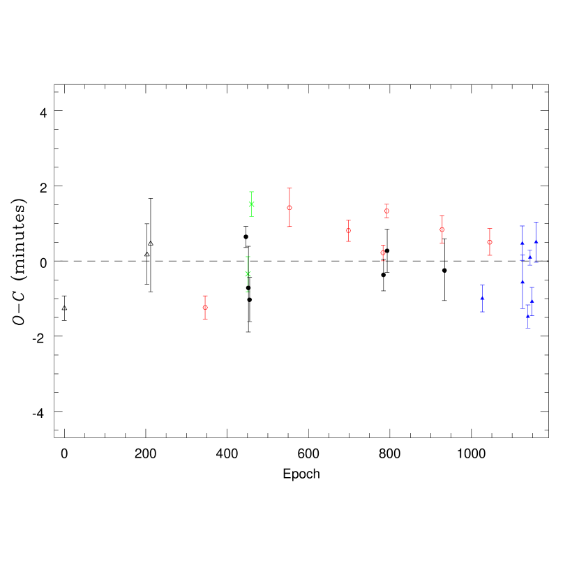
Figure 2: The $O-C$ diagram for the linear fitting. Here, the notations of the data points are as follows: filled black circles– our data points; open black triangles– Hartman et al. (2009); green crosses – Lee et al. (2012); red open hexagons– Mancini et al. (2018); and filled blue triangles – Alexoudi et al. (2018).

Figure 3: A periodogram showing the spectral power versus frequencies determined for all the data (new+published) used in this paper. The FAP for our largest power frequency is 61%. In the plot, the powers corresponding to the FAP values of 1% and 5% are also shown with dotted lines.

Figure 4: The $O-C$ diagram for one-frequency model The models is determined for $f=0.00790059461$ epoch^-1 The curve shows the fitting function. Among the data points, the filled black circles represent our data; open black triangles are for the Hartman et al. (2009) data; Lee et al. (2012) data is shown by green crosses; red open hexagons are for the Mancini et al. (2018) data points; and filled blue triangles represent the data from Alexoudi et al. (2018).

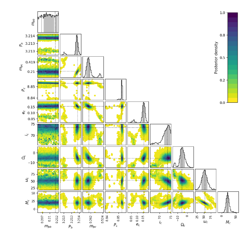
Figure 5: The MCMC posterior parameter distributions. Those with colors are pairwise two-dimensional projections. The one-dimensional projections are presented as the histograms on the top. The parameters shown here have one more subscript but their meanings and units are the same as those in Table LABEL:MC3input. The parameters with subscript ‘$b$’ are for the exoplanet HAT-P-12b, and those with subscript ‘$c$’ are for the exoplanet HAT-P-12c. The dotted lines indicate the parameter values of the best-fit model. The grey areas of histograms denote $68\%$ highest posterior density regions of the parameter distributions.

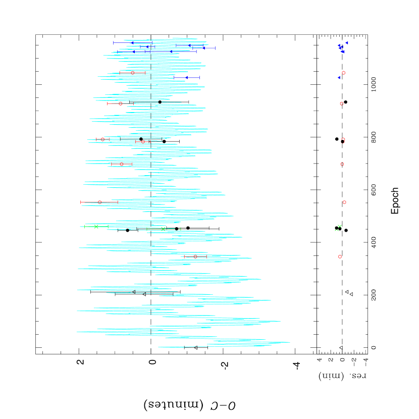
Figure 6: The $O-C$ diagram for the two-planet model. The curve shows the theoretical TTV and the points with error bars are the same as those shown in Fig. 2. The bottom panel shows a distribution of the fitting residuals between the data points and the model.