Abstract

Persistent homology is used to track the appearance and disappearance of features as we move through a nested sequence of topological spaces. Equating the nested sequence to a filtration and the appearance and disappearance of features to events, we show that simple event history methods can be used for the analysis of topological data. We propose a version of the well known Nelson-Aalen cumulative hazard estimator for the comparison of topological features of random fields and for testing parametric assumptions. We suggest a Cox proportional hazards approach for the analysis of embedded metric trees. The Nelson-Aalen method is illustrated on globally distributed climate data and on neutral hydrogen distribution in the Milky Way. The Cox method is use to compare vascular patterns in fundus images of the eyes of healthy and diabetic retinopathy patients.

Keywords: Betti numbers; Cumulative hazard; Counting process; Cox model; Persistent Homology; Simplicial complex

1 INTRODUCTION

Although interest in topological data analysis has grown sharply in recent years, most of the important developments have appeared outwith the statistical literature. We suggest that a consequence is that the potential benefits of adapting some established statistical methods to topological data may not have been fully exploited. In this paper we argue that event history methods are highly suitable for the analysis of data on certain topological features, that the use of such methods can increase the power and effectiveness of topological data analyses, and in turn that exploitation of topological features can bring added value to statistical analyses.

We use Fig. 1 and Fig. 2 to illustrate, at the cost of preempting Section 3, where they will be explained more fully. Figure 1 shows four simulated stationary and isotropic random fields, each on a $60\times 60$ discrete lattice. They are simulated to have correlation functions that are indistinguishable for practical purposes. All four have standard N(0,1) marginal distributions. Panel (a) is a simulation from a Gaussian random field, panels (b) and (c) are independent realisations of one particular non-Gaussian random field, and panel (d) is a realisation of a second non-Gaussian random field. Panel (d) is visually quite different from the others, but we see no obvious differences between (b) or (c) and the Gaussian random field (a). Figure 2 however shows simple Nelson-Aalen plots based on topological features of these data, to be described in Section 3. Now the differences are stark. Given that all four have the same marginal and correlation properties, we know of no other method that can draw out higher order differences so readily. Further, panel (a) is seen to be consistent with a Gaussian random field while the other panels are not.

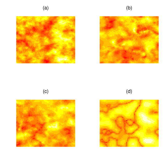
Figure 1: Four simulated random fields, each on a 60$\times$60 lattice.

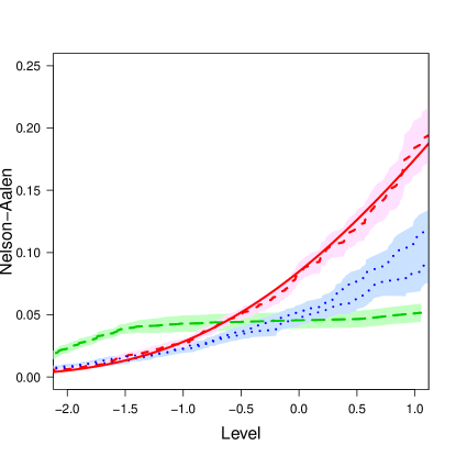
Figure 2: Nelson-Aalen plots for connected components for the random fields of Fig. 1. Short dashed lines correspond to panel (a), dotted lines to panels (b) and (c), and long dashed lines to panel (d). The shaded regions indicate $\pm$ one standard deviation. The solid line shows the expected value for a Gaussian random field with the same correlation structure as the data in Fig. 1.

Topological data analysis is in part founded on persistent homology. Important early contributions include Frosini (1992), Robins (1999) and, particularly, Edelsbrunner et al. (2002), who introduced the idea of persistence of features along filtrations. However, the earliest appearance of the expression “topological data analysis” seems not to have been until work by De Silva & Carlsson (2004) and Bremer et al. (2004). Later, Carlsson (2009) was key in the popularisation of topological data analysis, demonstrating how ideas from topology could solve many of the issues faced when applying geometric methods to complex data. Other developments are described by Perea (2019).

In Section 2 we give an introduction to the key constructs and concepts underpinning persistent homology and topological data analysis, aimed at a statistical reader. In Section 3 we develop the idea of Nelson-Aalen plots for topological features of random fields, as already seen in our introductory example. We apply the methods in two application areas, one being properties of climate model residuals on a sphere, and the other the distribution of neutral atomic hydrogen H i in the interstellar medium. In Section 4 we consider topological methods for embedded metric trees and propose Cox regression methods as a simple way to deal with potentially censored tree data. This method is applied to vascular structures in fundus images of the human eye, where it has potential to be an effective screening tool for the early detection of diseases.

2 TOPOLOGICAL DATA ANALYSIS

Topology is the study of features in a space that are invariant under continuous deformation. We will concentrate on topological data analysis methods that are based on persistent homology, which is the most popular variant of topological data analysis. Detailed descriptions are provided by, inter alia, Edelsbrunner et al. (2002), Edelsbrunner & Harer (2008), Carlsson (2009) and Edelsbrunner & Morozov (2012), with an excellent computational description given by Otter et al. (2017). Other variants of topological data analysis are summarised by Wasserman (2018).

We assume we have a metric space and inherited distance function. Dealing with arbitrary features in a space is complicated, and so a starting point is to give a representation in a common form. One such is a simplicial complex, which is a collection of vertices, edges, triangles, tetrahedra and higher dimensional equivalents. Thus the letters T, D, and A when written on a page could be represented by four vertices connected by three edges (T), a triangle (D) and a triangle with two extra external edges to two extra vertices (A). Simplicial complexes are not unique but they facilitate the use of linear algebra for the computation of topological invariants, which are features that do not change when the underyling space is bent, stretched or otherwise deformed, but without gluing or tearing.

The most important topological invariants are the homology groups, which are formally algebraic constructs, one per natural number, that collect together invariant features at each dimension. The ranks of these groups are called Betti numbers. The zero-dimension homology group $H_{0}(\mathcal{X})$ of a simplicial complex $\mathcal{X}$ consists of the disjoint elements, often referred to as connected components. For example, if the letters T, D, and A are written on a page then there are three connected components and the zero-order Betti number is $\beta_{0}=3$. In three dimensions, if we take for example letter balloons of T, D and A, there are still three connected components.

The next homology group $H_{1}(\mathcal{X})$ consists of holes constructed from one-dimensional edges. These are loops or cycles that cannot be shrunk to a single point. For T, D, and A on a page there are two, so $\beta_{1}=2$. For T, D, and A as letter balloons we have $\beta_{1}=4$. This is because the D and the A are each homologous to a torus. The hole through the centre of the torus is obvious: the other hole arises because a loop around the circle of revolution that forms the torus cannot be shrunk to a point without leaving the surface.

The second-dimension homology group $H_{2}(\mathcal{X})$ consists of two-dimensional cycles which enclose an empty three-dimensional space, often called a void. For T, D, and A in balloon form there are three, with one per connected component. For T, D, and A on a page there are none.

We now turn to persistent homology, which begins with a filtration of a space or simplicial complex $\mathcal{X}$. This is a nested sequence of subsets

$$\emptyset=\mathcal{X}_{0}\subseteq\mathcal{X}_{1}\subseteq\cdots\subseteq\mathcal{X}_{d}\cdots\subseteq\mathcal{X}_{n}=\mathcal{X},$$ (1)

indexed by a parameter $d$ that can be discrete or continuous. Each subset is itself a valid simplicial complex, with associated homology groups. Panel (a) of Fig. 3 illustrates. It shows a rooted metric tree embedded in two dimensions, and is a simplified version of the metric trees we will consider in Section 4. There are no cycles and so no holes. In this example the feature of interest is the connectivity of the tree as we move towards the root, filtering inward by radial distance. So $\mathcal{X}_{d}$ consists of the subset of $\mathcal{X}$ that is outside a circle of radius $r=1/d$ from the root. The plot shows two examples. The complex outside the outer circle consists of just one connected component. The complex outside the inner circle consists of nine connected components.

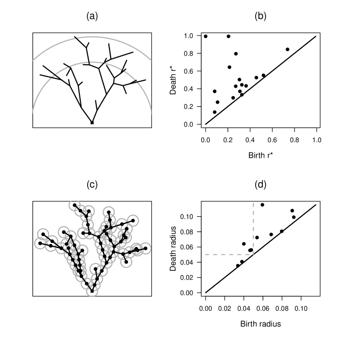
Figure 3: Illustrations of persistent homology: (a) embedded metric tree filtered by radius from root; (b) corresponding persistence diagram for connected components; (c) point cloud filtered by ball diameter; (d) corresponding persistence diagram for holes.

In persistent homology the appearance and disappearance of features is tracked as we move through the filtration. A feature is said to be born when it appears and to die when it disappears or merges with another feature. Thus if we start with $r=\infty$ in Fig. 3 there are no features. This continues as $r$ is decreased until it reaches the point on the tree that is furthest from the root, at radius $r_{\rm max}$ say. The first component is born at this level. As $r$ is decreased further, additional components are born at vertices that have only inward facing edges. Existing components merge at vertices with two outward facing edges. In these cases, by convention the component that was born first is assumed to continue, and the component that was born second is said to die at this radius. The process continues until the root is reached and the tree consists of a single connected component.

The birth and death levels of components are often represented by a persistence diagram, as in panel (b) of Fig. 3. This is a plot of birth times and death times of features as we move through the filtration. In the example we have plotted against $r_{\rm max}-r$ so that the first component to be born is on the left of the horizontal axis. Points near the diagonal are short-lived, points further from the diagonal are longer-lived. In the example we have two subtrees with common root, which merge only at $r=0$ and so there are two points with the same maximum death time.

A common way to represent a topological space is through a point cloud, as in panel (c) of Fig. 3. In these cases a filtration is usually defined by growing balls of increasing diameter, centred on the points. There are different ways of forming simplicial complexes in these cases, the most common of which is the Vietoris-Rips complex, which defines a subset of points to be a simplex in $\mathcal{X}_{d}$ when all pairwise distances between points are less than $2d$. The persistence diagram in panel (d) relates to the birth and death of holes for this example. The grey broken lines indicate the ball radius shown in (c). We see that a medium sized hole is about to be born towards the upper right and this will have modest persistence. A large hole in the centre will be born when the ball radius is increased a little more. This will be the last hole to die and is represented by the highest point in panel (d).

Topological data analysis is often used when there is a real-valued function $z_{x}$ associated with each point $x$ in a space $\mathcal{X}$. A lower level set $\mathcal{X}_{t}$ is defined as

$$\mathcal{X}_{t}=\{x:z_{x}\leq t,x\in\mathcal{X}\},$$ (2)

and upper level sets can defined similarly. A filtration is defined by increasing or decreasing the threshold $t$ and persistence of topological features in the level sets is tracked. Figure 4 illustrates. In panel (a) we show a two-dimensional image on a discrete $20\times 20$ grid. We assume that pixels that share an edge are connected but those that share only a vertex are not. Panels (b) and (c) show two level sets: pixels with image values less than $t=-1$ and less than $t=0$ respectively, marked as dark squares. In panel (b) there are $\beta_{0}=6$ connected components. There are also two regions in that panel that are not in the level set and are completely separated by connected components. Hence $\beta_{1}=2$. The level set has expanded by $t=0$ in (c) and the six previous components have merged, along with others, to form one large component. One new component has appeared to the lower left, and a small single-pixel component is close by, so $\beta_{0}=3$. Five holes are evident.

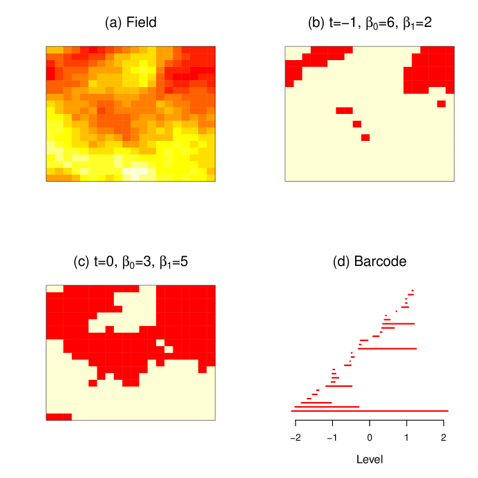
Figure 4: A simulated Gaussian random field together with level sets $\mathcal{X}_{-1}$ and $\mathcal{X}_{0}$, and barcode for connected components.

The final panel of Fig. 4 shows a so-called barcode for connected components for the image in panel (a). This is an alternative to a persistence diagram for the presentation of lifespans of topological features as we filter through the level sets. There is one line per feature, starting at the birth level and ending at the death level. In the example the lowest field value is in the dark region to the top right. This corresponds to the first pixel to appear in the level set, which by convention is the last to die, giving the long line at the bottom of the barcode in (d). The second component to be born is at a local minimum toward the top-left of the image. This component also has the second-longest lifetime until it merges with the first at around $t=-0.25$. The third-longest lifetime corresponds to the cluster at the lower left of the figure, which is relatively late to be born but quite isolated from other components and hence persists for some time.

A variety of approaches for the analysis of persistence diagrams and barcodes have been proposed. Wasserstein or bottleneck distances can be used to measure the difference between two persistence diagrams, but these measures are not calibrated to any interpretable scale. There remains no useful equivalents of, say, means or variances for persistence diagrams, which would be needed for inference. Mileyko et al. (2011), Turner et al. (2014) and Munch et al. (2015) showed how to obtain a Fréchet mean for a group of persistence diagrams, but unfortunately this is not unique. An alternative is to base inference on summaries such as the landscape functions of Bubenik (2015), which essentially consider nested profiles of the point patterns, or on counts of points over subregions, possibly with smoothing to produce the persistent images of, for example, Adams et al. (2015). Other proposals include a form of parametric bootstrap suggested by Adler et al. (2017) and the accumulated persistence suggestion of Biscio & Møller (2019). Wasserman (2018) provides a recent review. Our approach is quite different.

3 NELSON-AALEN FOR RANDOM FIELDS

3.1 Method

Let $\mathcal{Z}$ be a zero-mean real-valued random field defined on a finite discrete space $\mathcal{X}$. We assume a discrete space because in the applications we have in mind the field will often be an image, and invariably pixellated. Let $z_{x}$ be the field value at location $x\in\mathcal{X}$. We assume $z_{x}$ is drawn from a continuous distribution with no jump discontinuities and that there are no ties. We will require cor$(z_{x},z_{x^{\prime}})<1$ for all $x\neq x^{\prime}$ in $\mathcal{X}$.

Our filtration corresponding to (1) will be the nested sequence of sub-level sets (2). But instead of tracking the persistence of features, which underpins most published applications of topological data analysis, we will take a counting process approach based on the birth levels of new features in the filtration. As well as being computationally much more simple, the approach leads naturally to the use of methods that are familiar in event history analysis, with level playing the role of time and with negative values allowed. As features of interest we will concentrate here on connected components within $\mathcal{X}_{t}$, namely the $0$-dimensional features.

A component is born at location $x$ at level $t$ if $z_{x}=t$ and $x$ corresponds to a local minimum of $\mathcal{Z}$. To define a local minimum in the discrete space $\mathcal{X}$ we need to define the neighbours $(x)$ of each location $x$. We are free to do this as we wish, though shared edges or nearest neighbours seem sensible for pixellated or lattice-based fields.

Let $N_{x}(t)$ count the number of components that are born at location $x$ up to and including level $t$, and let $Y_{x}(t)$ be the associated predictable at-risk indicator. This is an indicator of whether, given the evolution of level sets to just before level $t$, it is possible for location $x$ to hold a local minimum at $t$. So

$$N_{x}(t)=\left\{\begin{array}[]{ll}1&z_{x}\leq t,\;\;z_{(x)}>z_{x}1_{x},\\ \\ 0&{\rm otherwise},\end{array}\right.\;\;\;\;\;\;\ Y_{x}(t)=\left\{\begin{array}[]{ll}1&z_{x}\geq t,\;\;z_{(x)}>t1_{x},\\ \\ 0&{\rm otherwise},\end{array}\right.$$

where $1_{x}$ is a unit vector of the same length as $z_{(x)}$. Define $N(t)=\sum_{x}N_{x}(t)$ and $Y(t)=\sum_{x}Y_{x}(t)$. Now let

$$\hat{A}(t)=\int_{-\infty}^{t}\frac{dN(u)}{Y(u)}.$$ (3)

This is an analogue of the Nelson-Aalen estimator of the cumulative hazard for a survival time variable (Aalen et al., 2008). If preferred, we can redefine the level scale $t$ to $t^{\ast}=\exp(t)$ so as to be a more familiar non-negative argument. Like the Nelson-Aalen estimator, $\hat{A}(t)$ is defined for all $t$ and has a finite number of discontinuities at the observed birth times. It is non-negative and uniformly bounded for fixed $\mathcal{X}$. It is a cadlag process, meaning continuous to the right with left limits. However, the standard Nelson-Aalen variance estimator

$${\hat{\rm{var}}\{\hat{A}(t)}\}=\int_{-\infty}^{t}\frac{dN(u)}{Y^{2}(u)}$$ (4)

does not in general apply, for a variety of reasons. One is possible non-independence between counting processes at different locations given non-independence of the underlying field values. Another, related, reason is informative censoring: knowledge that location $x$ falls out of the risk set at level $u$ provides information about other locations. And a third reason is that we have not constructed a martingale with respect to the observed data filtration.

We propose such Nelson-Aalen estimators for topological features as tools for comparing properties of fields beyond marginal and correlation structures, for comparing observed field data or model residuals with an assumed parametric model, and as a diagnostic for assumed or fitted correlation structures. We allow either a single field $\mathcal{Z}$ or independent and identically distributed replicates $\mathcal{Z}_{1},\mathcal{Z}_{2},\ldots,\mathcal{Z}_{N}$ defined on a common space $\mathcal{X}$.

3.2 Asymptotics

If $\mathcal{X}$ is fixed and there are $N$ independent replicates $\hat{A}_{1}(t),\ldots,\hat{A}_{N}(t)$, then as each $\hat{A}_{i}(t)$ is non-negative and bounded above, for each level $t$ the variance of $\hat{A}_{i}(t)$ is finite and the classic central limit theorem applies. Hence pointwise inference for large $N$ is straightforward, based on the sample mean $\bar{A}(t)$ and associated sample standard deviation.

For simultaneous confidence bounds we need to be a little careful because of the discontinuities in $\hat{A}_{i}(t)$. Hahn (1977) for instance points out that there can be uniformly bounded cadlag processes for which no central limit theorem applies, depending upon properties of their jumps. Bloznelis & Paulauskas (1994) provide sufficient conditions under which $\surd N\bar{A}(t)$ converges weakly to a Gaussian process with finite variance and smooth sample paths in $(0,\tau)$, for any arbitrarily large $\tau$ for which pr$\{Y(\tau)>0\}>0$. These conditions are verified in Supplementary Material. Hence a functional central limit theorem applies.

Further, for fixed $\mathcal{X}$ we can show that $\bar{A}(t)$ is consistent in $N$ for

$$A(t)=\displaystyle\int_{-\infty}^{t}J(u)\frac{\sum_{x}{\rm pr}(z_{(x)}>u1_{x}\mid z_{x}=u)f_{x}(u)}{\sum_{x}{\rm pr}(z_{x}>u,\;z_{(x)}>u1_{x})}du,$$ (5)

where $f_{x}(.)$ is the marginal density of $z_{x}$ and $J(u)=1$ if $E\{Y(u)\}>0$, zero otherwise. If $N=1$ and there is just a single realisation, the estimator $\hat{A}(t)$ is also consistent for (5), but this time as the cardinality of $\mathcal{X}$ increases, provided cor$(z_{x},z_{x^{\prime}})$ approaches zero as the distance between $x$ and $x^{\prime}$ increases.

3.3 Inference

For inference, we need to distinguish between the single and multiple replication situations. We will begin by assuming multiple replications: $\hat{A}_{1}(t),\ldots,\hat{A}_{N}(t)$.

We can consider the replicates $\hat{A}_{i}(t)$ as functional data. It is helpful to discretise the time/level scale of the estimator (3) to a grid of $M$ distinct levels $\tau_{1}=t_{1},\ldots,t_{M}=\tau_{2}$. This is a common assumption in functional data analysis and deals effectively with the discontinuities in our estimators, which with probability one will not occur at measurement points. There are then a huge array of analysis techniques immediately available: see for example the excellent review by Wang et al. (2016) for general approaches, and Chiou & Müller (2009) for a specific example of treating discretised hazards as functional data. With our applications in mind, we will mention only the construction of simultaneous confidence bands. This problem has had attention for functional data that are either sparse (Yao et al., 2005; Ma et al., 2012) or dense (Degras, 2011; Cao et al., 2012). Given that our discretisation is by design, a dense functional data approach is appropriate.

Let $\hat{A}_{ij}$ be the Nelson-Aalen estimator for field $\mathcal{Z}_{i}$ at level $t_{j}$. Let $\bar{A}_{j}$ and $\hat{\sigma}_{j}^{2}$ be the sample mean and sample variance of the estimators at $t_{j}$, and let $\hat{\rho}_{jk}$ be the estimated correlation between $\hat{A}_{.j}$ and $\hat{A}_{.k}$. Degras (2011) establishes that for fixed $\tau_{1}$ and $\tau_{2}$, as both $N$ and $M$ increase

$$\bar{A}_{j}\pm c_{\gamma}\hat{\sigma}_{j}/\surd N$$

has asymptotic coverage $1-\alpha$, where $c_{\alpha}$ is the upper $\alpha$-quantile of the maximum absolute value over $(\tau_{2}-\tau_{1})/\tau_{2}$ of a Gaussian process with standard margins and with correlation function equal to an appropriately scaled limit of $\hat{\rho}_{jk}$. The threshold $c_{\gamma}$ needs to be obtained numerically: software is available in the R package SCBmeanfd (Degras, 2016).

Turning to the case of a single replication only, we assume a parametric model $F_{\theta}$ is available for the random field $\mathcal{Z}$ and we propose a parametric bootstrap approach. Parametric and more general bootstrap methods for functional data have been studied empirically and theoretically by, for example, Cuevas et al. (2006). We require a consistent estimator $\hat{\theta}$ of the parameter vector $\theta$. We then generate $B$ simulated realisations of $\mathcal{Z}$ on $\mathcal{X}$ from $F_{\hat{\theta}}$, and obtain the bootstrap Nelson-Aalen estimators $\hat{A}_{b}(t)$ for $b=1,\ldots,B$. Pointwise intervals that have correct coverage asymptotically in $B$ and $\mid\mathcal{X}\mid$ can be obtained from the bootstrap quantiles or a Normal approximation justified by the central limit theorem.

For simultaneous confidence bands we suggest a Monte Carlo method used by Crainiceanu et al. (2011) that avoids explicit estimation of the correlation function. We again discretise the original and bootstrap estimators $\hat{A}_{b}(t)$ to a dense grid of $M$ points over a fixed range of levels $(\tau_{1},\tau_{2})$. Let $\hat{A}_{j}$ be the Nelson-Aalen estimate (3) at level $t_{j}$ obtained from the original data, and let $\hat{A}_{bj}$ be corresponding value from bootstrap replicate $b$. Let $\bar{A}_{j}$ and $\hat{\sigma}_{j}$ be the bootstrap mean and estimated standard deviation at $t_{j}$. Define

$$G_{b}=\max_{j}\{\mid\hat{A}_{bj}-\bar{A}_{j}\mid/\hat{\sigma}_{j}\},$$

and take $\hat{d}_{\alpha}$ to be the upper $\alpha$-quantile of the empirical distribution of $G_{1},\ldots,G_{B}$. Then for large $M$ an approximate simultaneous confidence band for $A(t)$ over $(\tau_{1},\tau_{2})$ is

$$\hat{A}_{j}\pm\hat{d}_{\alpha}\hat{\sigma}_{j}\hskip 28.45274ptj=1,\ldots,M.$$

3.4 Simulation studies

We consider random fields on $d\times d$ lattices and investigate three models. The first, M1, is a stationary and isotropic Gaussian random field with standard N(0,1) marginals and Matérn correlation function. If locations $x$ and $x^{\prime}$ are separated by Euclidean distance $u$ then

$$\mbox{cor}\left(z_{x},z_{x^{\prime}}\right)=\frac{2^{1-\nu}}{\Gamma(\nu)}\left(\sqrt{2\nu}u/\eta\right)^{\nu}K_{\nu}\left(\sqrt{2\nu}u/\eta\right),$$

where $K_{\nu}(.)$ is a modified Bessel function of the third kind. Let $\theta_{1}=(\eta,\nu)$.

The second model, M2, is a marginally transformed $\chi^{2}_{1}$ field. We simulate from the Gaussian random field model M1, with parameters $\theta_{2}$. Values are then squared to give $\chi^{2}_{1}$ margins. Let $y_{x}$ be the value at location $x$. We next marginally transform to N(0,1) using $z_{x}=\Phi^{-1}\{F_{1}(y_{x})\}$, where $\Phi(.)$ and $F_{1}(.)$ are the N(0,1) and $\chi^{2}_{1}$ cumulative distribution functions, respectively.

The third model, M3, is a marginally transformed $F_{3,3}$ field. We begin by constructing two independent $\chi^{2}_{3}$ fields, each from the sum of three squared independent Gaussian random fields M1 with Matérn parameters $\theta_{3}$. The ratio of these $\chi^{2}_{3}$ fields has $F_{3,3}$ distribution and we again marginally transform back to N(0,1).

All simulated fields are mean-corrected to help with the comparisons. The purpose of the marginal transformations is to generate fields that are not Gaussian random fields but which have Gaussian N(0,1) marginal distributions. This is so that we can assess the added value of topological methods over and above simple comparisons of marginal distributions. Similarly, in our simulations, for each choice of correlation $\theta_{1}$ for model M1 we choose $\theta_{2}$ and $\theta_{3}$ so as to match as closely as we can the correlation of the final M2 and M3 fields to Matérn with parameters $\theta_{1}$. Details of this are presented in Supplementary Material. Again, the point is to show that differences between fields are not explained by differences in correlation functions. We have no particular interest in M2 and M3 other than as easily generated non-Gaussian random fields to be used as comparators.

The previously-presented Fig. 1 gives in panel (a) an example simulation from M1 on a $60\times 60$ lattice with $\theta=(5,1).$ Panels (b) and (c) provide two examples of M3, and panel (d) an example of M2, with matched correlations. The topological Nelson-Aalen plots for these fields are in Fig. 2. The solid line is the limiting value (5), which we obtained using the multivariate Gaussian distribution function routine in the R package mvtnorm.

Table 1 shows coverage of nominal 95% confidence intervals and bands based on Nelson-Aalen plots for connected components from Gaussian random fields M1 simulated on a 60$\times$60 lattice. Pointwise coverage is evaluated at selected percentiles of the at-risk distributions, ie levels $t$ satisfying $E\{Y_{x}(t)\}=p$ for five different values of $p$. The simultaneous confidence bands cover the central 90% of the at-risk distributions, discretised to a grid of 200 equally spaced points. For each parameter combination we give results for three methods. The first, for reference, is a naive approach that assumes standard methods based on the variance estimator (4) can be applied and using Bie et al. (1987) for simultaneous confidence bands. The second method assumes we have a single replication and uses a parametric bootstrap with $B=200$ simulated Gaussian random fields, generated with Matérn correlation parameters taken as the maximum likelihood estimates from the sole replicate. The third method assumes we have replicates. The standard and parametric bootstrap results are based on 1000 single simulations, the results with replications are from 1000 batches of $N=40$ replicates, which matches an application in the next subsection. There is severe undercoverage at times for the standard confidence intervals, but the other methods both produce good results.

Simulation results for M2 and M3 are provided in Supplementary Material, along with further simulations to assess size and power when using our method to test for a Gaussian random field.

Table 1: Coverage of nominal 95% pointwise confidence intervals and 95% simultaneous confidence band (SCB) around Nelson-Aalen component plots for Gaussian random fields. Results from 1000 simulations on $60\times 60$ lattices, with Matérn correlation function with parameters $\eta$ and $\nu$

		Percentile
$(\eta,\nu)$	Method	0.9	0.7	0.5	0.3	0.1	SCB
(5,1)	Standard	84.0	92.2	93.5	88.9	82.2	73.9
	Par. bootstrap	95.3	94.4	95.8	95.3	96.2	94.1
	Replications	94.2	94.7	95.7	93.9	94.7	94.4
(10,1)	Standard	67.8	82.7	83.3	73.7	65.5	39.1
	Par. bootstrap	95.3	95.1	95.6	95.7	94.7	93.6
	Replications	95.1	94.0	94.9	95.9	94.0	96.4
(5,2)	Standard	93.4	94.6	95.0	93.2	90.8	82.9
	Par. bootstrap	95.4	95.2	95.7	95.5	95.8	95.9
	Replications	94.0	94.6	95.0	94.3	93.7	93.4

In Table 2 we provide a brief comparison between using the proposed Nelson-Aalen estimator and existing topological data analysis techniques when discriminating between random fields, all on 60$\times$60 lattices. The statistical properties of topological summaries such as persistence diagrams and landscape functions are not understood, which means we cannot use these methods to assess the adequacy of an assumed model such as a Gaussian random field, or for single-sample problems. However, if we have two or more groups of replicated data we can compare classification performance.

We took training data to be batches of 40 random fields simulated from models M1, M2 and M3, for each of the three parameter choices. We then used a support vector machine to develop pairwise probabilistic classifiers, using the default parameter choices for the svm routine in the R package e1071. We built classifiers based on the proposed Nelson-Aalen estimator $\hat{A}(t)$ defined at (3) and on the first 10 landscape functions (Bubenik, 2015) for each of components and holes, choosing the best of these to compare with $\hat{A}(t)$. Landscape functions are popular summaries of persistence diagrams and are available through the R package TDA. We replicated the training data 20 times and assessed classifier performance on separate groups of 200 simulated random fields for each model.

We assume test data would be allocated to the group with the highest class probability. In Table 2 we provide the accuracy of the classifier, which is the proportion of test data that are allocated to the correct group, and as a calibration measure we give the mean class probabilities for the correct groups. For example, a classifier that estimates the probability of the correct group to be 0.51 gives accurate allocation but is poorly calibrated, whereas one that estimates the correct class probability to be 0.99 would be both accurate and well calibrated. The table shows that classification based on the Nelson-Aalen estimator consistently outperforms classification based on the landscape functions in both accuracy and calibration. Additional simulation results provided in Supplementary Material support this conclusion.

Table 2: Classification of random fields. Accuracy (Acc.) measures the proportion of random fields that were correctly allocated and calibration (Cal.) gives the mean estimated class probabilities for the correct classes. Values are multiplied by 100 for presentation

Matérn	Method	M1 v M2		M1 v M3		M2 v M3
$(\eta,\nu)$		Acc.	Cal.	Acc.	Cal.	Acc.	Cal.
(5,1)	Nelson-Aalen	100.0	97.7	99.4	96.6	100.0	97.5
	Landscape	96.5	92.5	91.7	85.5	95.4	91.6
(10,1)	Nelson-Aalen	99.7	97.2	95.2	91.0	100.0	97.3
	Landscape	99.7	97.0	80.7	72.0	95.8	90.1
(5,2)	Nelson-Aalen	100.0	97.6	99.7	97.1	100.0	97.4
	Landscape	92.3	87.7	79.4	71.0	87.5	80.1

3.5 Applications: climate modelling, interstellar medium

The Community Earth System Model Large Ensemble project (Kay et al., 2015) is a publicly available ensemble of 40 high resolution climate model simulations. Although the models used to generate the data are deterministic, spatial and spatio-temporal statistical modelling is often applied as a means to both explore and concisely summarise the output (Castruccio, 2016; Edwards et al., 2019). Such models often assume that the modelled residuals form a Gaussian random field. We can use the topological Nelson-Aalen approach to assess this assumption, at least in part, and as a quick and easy method to compare ensemble members and to examine the suitability of assumed correlation structures.

To illustrate our method we considered annual wind intensities at $10$m for the year 2020. Each ensemble member has data on a 192$\times$288 grid over the surface of a sphere and at each data point we standardised by the mean and standard deviation across members. To keep the correlation matrices manageable for this illustration we used every third lattice point in both the latitudinal and longitudinal directions. Following Castruccio & Genton (2014) and Castruccio & Genton (2016) we also trimmed the regions near the poles, leaving data on a $51\times 96$ lattice for each ensemble member.

Topological Nelson-Aalen plots for connected components are shown as functional boxplots (Sun & Genton, 2011) in the left panel of Fig. 5 together with a simultaneous confidence band for the mean. There is reassurance that the standard assumption of a Gaussian random field for these climate residuals is reasonable: the band almost uniformly includes the expected value for a Gaussian random field with correlation function taken to be the empirical correlation found in the data. To illustrate the potential of our method as a diagnostic for fitted correlation models, the figure also includes expected values under three modelled correlation structures. These are the three dotted lines in the plot. In order from the top, the first line corresponds to a stationary Matérn model. It is clearly poor for these data, and the same is true for the second dotted line, which corresponds to a regional block model with separate Matérn correlation functions fitted to land, ocean and coastal regions. In contrast, as seen by the lowest dotted line, a semiparametric non-stationary model proposed by Konzen et al. (2019) fits these data well.

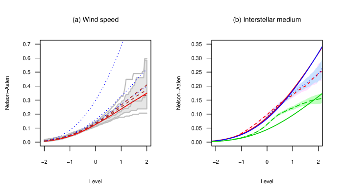
Figure 5: Nelson-Aalen plots for connected components. In (a) the grey region and lines represent functional boxplots of 40 separate realisations of climate data residuals. The long dashed lines represent the mean and associated 95% simultaneous confidence band, and the other lines are limiting values for Gaussian random fields with different correlation matrices. The solid line uses the empirical correlation matrix, the others are explained in the text. Panel (b) considers the neutral hydrogen data: the short dashed lines are Region 1, the dotted lines Region 2 and the long dashed lines Region 3. The shaded regions indicate $\pm$ two standard deviations. The solid lines show the limiting values for Gaussian random fields with matched correlations. The upper lines, which are almost indistinguishable, are for Regions 1 and 2, the lower is for Region 3.

Our second application is into the distribution in the Milky Way of neutral atomic hydrogen, H i, using data obtained by the Galactic All-Sky Survey using the Parkes 64 m radio telescope (McClure-Griffiths et al., 2009; Kalberla et al., 2010). Neutral atomic hydrogen makes up around 90% of the atoms in the interstellar medium, which embeds stars and galaxies. Turbulence and shocks lead to a highly heterogeneous random pattern to the local density of H i, and a common assumption in astrophysics is that after the removal of trends and large-scale features, the distribution of the log-density of H i is that of a Gaussian random field (Elmegreen & Scalo, 2004; Monin & Yaglom, 2007). This assumption was investigated by Henderson et al. (2020), who considered topological features of three distinct regions of the southern sky. Based on counts of components and holes, but not event history, the authors concluded that two regions were consistent, after monotonic transformation, with Gaussian random fields but the third was not.

The right panel of Fig. 5 shows Nelson-Aalen plots for connected components for these data. Each region consists of density measurements over a 256$\times$256 lattice and following Henderson et al. (2020) we considered the residuals after trend removal using a thin plate smoothing spline. The data were again marginally transformed to N(0,1) to preempt questions as to whether simple monotonic transformations could suffice to convert the data to Gaussian random fields. Region 3 is clearly distinct from the others and not consistent with the fitted Gaussian random field. Regions 1 and 2 have very similar Nelson-Aalen plots and almost indistinguishable limiting values for Gaussian random fields with Matérn correlations fitted to the data. There is evidence however that at the higher levels these regions are not consistent with the fitted Gaussian random fields.

4 COX PROPORTIONAL HAZARDS FOR EMBEDDED METRIC TREES

4.1 Topology and event history for tree data

We now turn to trees $\mathcal{T}=\{\mathcal{N},\mathcal{E}\}$ made up of nodes $\mathcal{N}$ and associated edges $\mathcal{E}$ embedded in $\mathbb{R}^{2}$ or $\mathbb{R}^{3}$, and with a single common ancestor. A simple example was shown in panel (a) of Fig. 3.

A number of approaches for the comparison of tree structures have been inspired by persistent homology. Kanari et al. (2018) considered persistence of one-dimensional features on contours equidistant from the root, whether path length or radial distance, as previously illustrated in Panel (a) of Fig. 3. Li et al. (2017b) independently proposed a similar approach in the comparison of neuronal tree structures. Bendich et al. (2016) applied persistent homology methods to brain artery trees in $\mathbb{R}^{3}$, Li et al. (2017a) used a geodesic distance function to derive persistence diagrams for the branching architectures of plants, and Brodzki et al. (2018) used persistent homology to classify bronchial trees.

None of the methods of which we are aware can deal with the possibility of censored or incomplete trees. For example, an image may capture only part of a tree, in which case edges that cross the image boundary would not be fully observed. Edges that reach the boundary are not true first order nodes or leaves, and should not be considered as birth or death locations when applying any of the persistent homological techniques. Equally they do contain information and these edges should not be ignored or discarded.

This type of problem is of course fundamental to event history and survival analysis methodology, where methods for censored or truncated data are very well established. Hence our proposal is straightforward: construct a filtration as above but consider as an event the occurrence of either a leaf or a branching point. More specifically we propose the following.

1. Filter outwards by radial distance $r$.

2. Consider a leaf event to occur at $r$ if a known leaf has that radial distance from the root. Consider a branch event similarly. If desired, we might distinguish bifurcations from trifurcations and so on. Censored points cannot be events.

3. Construct a risk set consisting of all edges in $\mathcal{E}$ that intersect a circle of radius $r$ centered at the root, as in panel (a) of Fig. 3.

4. Use standard event history methods to contrast events with risk sets.

Let $\mathcal{C}_{r}$ be a disc of radius $r$ centred on the root and define $\mathcal{T}_{r}=\mathcal{T}\cap\mathcal{C}_{r}$. Covariates can be included provided they are exogenous or dynamically defined on $\mathcal{C}_{r}$. Thus spatial location, branch order, edge weights, proximity to other branches in $\mathcal{C}_{r}$ and so on can be handled easily using a Cox or other event time regression model. Further, we can construct risk sets from multiple trees and use fixed or random effects (frailties) to include tree-to-tree comparisons.

For this method to work we need three common event history assumptions. First, that events occur independently given the risk sets and covariates. Second, that censoring is independent. Third, that whichever hazard or intensity model is assumed is appropriate. Under these assumptions standard results apply, including asymptotics for Cox or other model estimates.

4.2 Application: vascular patterns in the eye

The left panel of Fig. 6 shows the vascular pattern of a human eye, taken from a high dimensional image provided by Budai et al. (2013). The right panel of the figure shows a tree representation, with vertices joined by linear edges, a simplification of the optic nerve area to provide a root, and with the omission of vessels that appear to originate outwith the plot region. Vessels that reach the boundary of the plot region are marked as censored points. This is a two-dimensional projection of a three-dimensional tree and branches can cross. There are no cycles.

Figure 6: Left panel: vascular patterns in a healthy human eye, with data taken from Budai et al. (2013). Right panel: tree representation. Censored edges are marked by points.

The data in Fig. 6 are from one of the 15 fundus images of eyes of healthy patients provided by Budai et al. (2013), who also give fundus images of 15 patients with diabetic retinopathy. We use our methods to compare diabetic retinopathy and healthy patients, and also to investigate the effect of a number of covariates. These are the width of the vessel, the Euclidean distance between nodes, the ratio of path length to Euclidean distance between nodes as a measure of curvature, the number of other nodes within radius 200 units of the current node (about 10% of the image size), the generation order, and the azimuth to the root measured from the vertical. We assumed log-linear effects for all covariates except azimuth, for which we assumed a smooth effect via a $P$-spline with four degrees of freedom. We also included patient-level terms as either fixed effects or frailties. In total over the 30 patients there were 12590 edges. At this large sample size the fixed effect and frailty model fits were almost identical.

Table 3 summarises some of the results. In the upper part we consider an event to be the termination of a vessel at a leaf, and in the lower part we consider branching points. Given the large sample, statistical significance is almost irrelevant and so to compare the magnitudes of effects we take the hazard ratio (hr) between the 20% and 80% points of the covariate distributions.

As might be expected, large vessels are highly unlikely to terminate in a leaf but are more likely to branch. The hazard functions for both types of event fall as Euclidean distance from an earlier node increases. There is no real effect of either curvature of an edge or proximity to other nodes, but there is some evidence that branching becomes less likely as the generation of an edge increases. There is a modest azimuth effect on branching, with a plot of the smooth fit (not shown here) indicating a decrease in branching hazard as aziumth moves away from the vertical, fairly symmetrically in both directions.

Of most interest is the difference between patients. The estimated frailty terms for both leaf and branch events are shown in Fig. 7. There are relatively small differences between patients in vessel branching frequency, but large differences in the hazard for terminating in a leaf, given covariate effects. Interestingly, we have complete separation between healthy and diabetic retinopathy patients in these frailties.

Table 3: Cox proportional hazards results for eye trees

	Event = leaf
	Coefficient	SE	$\chi^{2}$	df	hr
Width	-0.3849	0.0079	2369.51	1	0.02
Euclid	-0.0051	0.0002	797.16	1	0.41
Path length ratio	1.0142	0.1260	64.76	1	1.05
Nodes within 200	0.0037	0.0037	1.02	1	1.02
Order	-0.0147	0.0049	8.90	1	0.86
Azimuth			34.66	4	1.18
Patient effect			823.98	29	2.29
	Event = branch
	Coefficient	SE	$\chi^{2}$	df	hr
Width	0.0591	0.0016	1420.28	1	1.88
Euclid	-0.0058	0.0001	1874.37	1	0.37
Path length ratio	-0.9058	0.2406	14.18	1	0.95
Nodes within 200	0.0375	0.0033	128.54	1	1.21
Order	-0.0622	0.0051	149.35	1	0.54
Azimuth			119.30	4	1.41
Patient effect			103.60	29	1.37

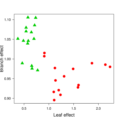
Figure 7: Subject-level frailties for 15 diabetic retinopathy patients (triangles) and 15 healthy patients (circles).

5 DISCUSSION

There are a number of areas for further work. In Section 3 we suggested empirical variances for the Nelson-Aalen estimator when there are repeated samples of random fields, as in the climate example, and parametric bootstrap estimators when there was interest in a particular model, such as a Gaussian random field. In Supplementary Material, an adjusted parametric bootstrap assuming local misspecification as in Copas & Eguchi (2005) is suggested and provides a conservative approach for the case of a single sample and no model. However, it would be useful formally to develop a non-parametric variance estimator.

In both Section 3 and Section 4 we concentrated on the birth times of connected components. We might also consider death times, though the identification of risk sets is less straightforward in this case, which in turn means that limiting properties will be harder to derive. For complexes in two or higher dimensions, including the random fields of Section 3, we could consider higher order features. In two-dimensions it will be particularly simple to use our methods to investigate death times of holes, which as a result of Alexander duality (Edelsbrunner & Kerber, 2012) can be analysed in the same manner as births of components simply by reversing the direction of the filtration.

6 ACKNOWLEDGEMENT

We thank Evandro Konzen and Jian Shi for providing software to fit their non-stationary correlation model to the climate data.

References

- Aalen et al. (2008) Aalen, O., Borgan, O. & Gjessing, H. (2008). Survival and Event History Analysis. New York: Springer.
- Adams et al. (2015) Adams, H., Chepushtanova, S., Emerson, T., Hanson, E., Kirby, M., Motta, F., Neville, R., Peterson, C., Shipman, P. & Ziegelmeier, L. (2015). Persistence images: a stable vector representation of persistent homology. arXiv , 1507.06217.
- Adler et al. (2017) Adler, R., Agami, S. & Pranav, S. (2017). Modeling and replicating statistical topology and evidence for cmb nonhomogeneity. Proc. Nat. Acad. Sci. 114, 11878–11883.
- Bendich et al. (2016) Bendich, P., Marron, J., Miller, E., Pieloch, A. & Skwerer, S. (2016). Persistent homology analysis of brain artery trees. Ann. App. Statist. 10, 198–218.
- Bie et al. (1987) Bie, O., Borgan, Ø. & Liestøl, K. (1987). Confidence intervals and confidence bands for the cumulative hazard rate function and their small sample properties. Scan. J. Statist. 14, 221–233.
- Biscio & Møller (2019) Biscio, A. & Møller, J. (2019). The accumulated persistence function, a new useful functional summary statistic for topological data analysis, with a view to brain artery trees and spatial point process applications. J. Comp. Graph. Statist 28, 671–681.
- Bloznelis & Paulauskas (1994) Bloznelis, M. & Paulauskas, V. (1994). A note on the central limit theorem for stochastically continuous processes. Stoch. Proc. Appl. 53, 351–361.
- Bremer et al. (2004) Bremer, P.-T., Hamann, B., Edelsbrunner, H. & Pascucci, V. (2004). A topological hierarchy for functions on triangulated surfaces. IEEE Trans. Vis. Comp. Graph. 10, 385–396.
- Brodzki et al. (2018) Brodzki, J., Guillamon, F. B., Djukanovic, R., Conway, J., Pirashvili, M. & Bennett, M. (2018). Lung topology characteristics in patients with chronic obstructive pulmonary disease. Sci. Rep. 8, 1–12.
- Bubenik (2015) Bubenik, P. (2015). Statistical topological data analysis using persistence landscapes. J. Mach. Learn. Res. 16, 77–102.
- Budai et al. (2013) Budai, A., Bock, R., Maier, A., Hornegger, J. & Michelson, G. (2013). Robust vessel segmentation in fundus images. Int. J. of Biomed. Imag. , http://dx.doi.org/10.1155/2013/154860.
- Cao et al. (2012) Cao, G., Yang, L. & Todem, D. (2012). Simultaneous inference for the mean function based on dense functional data. J. Nonpar.. Statist. 24, 359–377.
- Carlsson (2009) Carlsson, G. (2009). Topology and data. Bull. Am. Math. Soc. 46, 255–308.
- Castruccio (2016) Castruccio, S. (2016). Assessing the spatio-temporal structure of annual and seasonal surface temperature for cmip5 and reanalysis. Spat. Statist. 18, 179–193.
- Castruccio & Genton (2014) Castruccio, S. & Genton, M. G. (2014). Beyond axial symmetry: an improved class of models for global data. Stat 3, 48–55.
- Castruccio & Genton (2016) Castruccio, S. & Genton, M. G. (2016). Compressing an ensemble with statistical models: an algorithm for global 3d spatio-temporal temperature. Technometrics 58, 319–328.
- Chiou & Müller (2009) Chiou, J. & Müller, H. (2009). Modeling hazard rates as functional data for the analysis of cohort lifetables and mortality forecasting. J. Am. Statist. Assoc. 104, 572–585.
- Copas & Eguchi (2005) Copas, J. & Eguchi, S. (2005). Local model uncertainty and incomplete-data bias. J. Roy. Statist. Soc. B 67, 459–513.
- Crainiceanu et al. (2011) Crainiceanu, C., Staicu, A.-M., Ray, S. & Punjabi, N. (2011). Bootstrap-based inference on the difference in the means of two correlated processes. Statist. Med. 31, 3223–3240.
- Cuevas et al. (2006) Cuevas, A., Febrero, M. & Fraiman, R. (2006). On the use of the bootstrap for estimating functions with functional data. Comp. Statist. Dat. Anal. 51, 1063–1074.
- De Silva & Carlsson (2004) De Silva, V. & Carlsson, G. E. (2004). Topological estimation using witness complexes. In Eurographics Symposium on Point-Based Graphics. ETH, Zurich.
- Degras (2011) Degras, D. (2011). Simultaneous confidence bands for nonparametric regression with functional data. Statist. Sin. 21, 1735–1765.
- Degras (2016) Degras, D. (2016). SCBmeanfd: Simultaneous Confidence Bands for the Mean of Functional Data. R package version 1.2.2.
- Edelsbrunner et al. (2002) Edelsbrunner, Letscher & Zomorodian (2002). Topological persistence and simplification. Disc. Comp. Geom. 28, 511–533.
- Edelsbrunner & Harer (2008) Edelsbrunner, H. & Harer, J. (2008). Persistent homology -— a survey. In Surveys on Discrete and Computational Geometry, vol. 453. American Mathematical Society.
- Edelsbrunner & Kerber (2012) Edelsbrunner, H. & Kerber, M. (2012). Alexander duality for functions: The persistent behavior of land and water and shore. In Proceedings of the Twenty-Eighth Annual Symposium on Computational Geometry. Association for Computing Machinery.
- Edelsbrunner & Morozov (2012) Edelsbrunner, H. & Morozov, D. (2012). Persistent homology: Theory and practice. In Proceedings of the European Congress of Mathematics, Cracow.
- Edwards et al. (2019) Edwards, M., Castruccio, S. & Hammerling, D. (2019). A multivariate global spatiotemporal stochastic generator for climate ensembles. J. Ag. Biol. Env. Statist. 24, 464–483.
- Elmegreen & Scalo (2004) Elmegreen, B. G. & Scalo, J. (2004). Interstellar turbulence I: observations and processes. Ann. Rev. Astron. Astrophys. 42, 211–273.
- Frosini (1992) Frosini, P. (1992). Measuring shapes by size functions. In Intelligent Robots and Computer Vision X: Algorithms and Techniques, vol. 1607. International Society for Optics and Photonics.
- Hahn (1977) Hahn, M. (1977). Conditions for sample continuity and the Central Limit Theorem. Ann. Prob. 5, 351–360.
- Henderson et al. (2020) Henderson, R., Makarenko, I., Bushby, P., Fletcher, A. & Shukurov, A. (2020). Statistical topology and the random interstellar medium. J. Am. Statist. Assoc. 115, 625–625.
- Kalberla et al. (2010) Kalberla, P., McClure-Griffiths, N., Pisano, D., Calabretta, M., Alyson Ford, H., Lockman, F., Staveley-Smith, L., Kerp, J., Winkel, B., Murphy, T. & Newton-McGee, K. (2010). GASS: the Parkes Galactic all-sky survey II. Stray-radiation correction and second data release. Astron. Astrophys. 521, A17. doi.org/10.1051/0004-6361/200913979.
- Kanari et al. (2018) Kanari, L., Dlotko, P., Scolamiero, M., Levi, R., Shillcock, J., Hess, K. & Markram, H. (2018). A topological representation of branching neuronal morphologies. Neuroinformatics 16, 3–13.
- Kay et al. (2015) Kay, J. E., Deser, C., Phillips, A., Mai, A., Hannay, C., Strand, G., Arblaster, J. M., Bates, S., Danabasoglu, G., Edwards, J. et al. (2015). The Community Earth System Model (CESM) large ensemble project: A community resource for studying climate change in the presence of internal climate variability. Bull. Am. Met. Soc. 96, 1333–1349.
- Konzen et al. (2019) Konzen, E., Shi, J. & Wang, Z. (2019). Modelling function-valued processes with nonseparable covariance structure. arXiv , 1903.09981.
- Li et al. (2017a) Li, M., Duncan, K. J. K., Topp, C. N. & Chitwood, D. H. (2017a). Persistent homology and the branching topologies of plants. Am. J. Bot. 104, 349–353.
- Li et al. (2017b) Li, Y., Wang, D., Ascoli, G. A., Mitra, P. & Wang, Y. (2017b). Metrics for comparing neuronal tree shapes based on persistent homology. PLOS ONE 12. doi.org/10.1371/journal.pone.0182184.
- Ma et al. (2012) Ma, S., Yang, L. & Carroll, R. (2012). A simultaneous confidence band for sparse functional data. Statist. Sin. 22, 95–122.
- McClure-Griffiths et al. (2009) McClure-Griffiths, N., Pisano, D., Calabretta, M., Alyson Ford, H., Lockman, F., Staveley-Smith, L., Kalberla, P., Bailin, J., Dedes, L., Janowieck, S., Gibson, B., Murphy, T., Nakanishi, H. & Newton-McGee, K. (2009). GASS: the Parkes Galactic all-sky survey I. Survey description, goals, and initial data release. Astrophys. J. Supp. 181, 398–412.
- Mileyko et al. (2011) Mileyko, Y., Mukherjee, S. & Harer, J. (2011). Probability measures on the space of persistence diagrams. Inv. Prob. 27, 124007.
- Monin & Yaglom (2007) Monin, A. S. & Yaglom, A. M. (2007). Statistical Fluid Mechanics: Mechanics of Turbulence, Vols I and II. Mineola: Dover.
- Munch et al. (2015) Munch, E., Turner, K., Bendich, P., Mukherjee, S., Mattingly, J. & Harer, J. (2015). Probabilistic Fréchet means for time varying persistence diagrams. Elec. J. Statist. 9, 1173–1204.
- Otter et al. (2017) Otter, N., Porter, M. A., Tillmann, U., Grindrod, P. & Harrington, H. A. (2017). A roadmap for the computation of persistent homology. EPJ Dat. Sci. 6, 17. doi.org/10.1140/epjds/s13688-017-0109-5.
- Perea (2019) Perea, J. (2019). A brief history of persistence. Morfismos 23, 1–16.
- Robins (1999) Robins, V. (1999). Towards computing homology from finite approximations. Topol. Proc. 24, 503–532.
- Sun & Genton (2011) Sun, Y. & Genton, M. G. (2011). Functional boxplots. J. Comp. Graph. Statist. 20, 316–334.
- Turner et al. (2014) Turner, K., Mileyko, Y., Mukherjee, S. & Harer, J. (2014). Fréchet means for distributions of persistence diagrams. Disc. Comp. Geom. 52, 44–70.
- Wang et al. (2016) Wang, J.-L., Chiou, J.-M. & Müller, H.-G. (2016). Functional data analysis. Ann. Rev. Statist. Appl. 3, 257–295.
- Wasserman (2018) Wasserman, L. (2018). Topological data analysis. Ann. Rev. Statist. Appl. 5, 501–532.
- Yao et al. (2005) Yao, F., Müller, H.-G. & Wang, J.-L. (2005). Functional data analysis for sparse longitudinal data. J. Am. Statist. Assoc. 100, 577–590.