Exact Ground States and Domain Walls in One Dimensional Chiral Magnets

Abstract

We determine exactly the phase structure of a chiral magnet in one spatial dimension with the Dzyaloshinskii-Moriya (DM) interaction and a potential that is a function of the third component of the magnetization vector, $n_{3}$, with a Zeeman (linear with the coefficient $B$) term and an anisotropy (quadratic with the coefficient $A$) term, constrained so that $2A\leq|B|$. For large values of potential parameters $A$ and $B$, the system is in one of the ferromagnetic phases, whereas it is in the spiral phase for small values. In the spiral phase we find a continuum of spiral solutions, which are one-dimensionally modulated solutions with various periods. The ground state is determined as the spiral solution with the lowest average energy density. As the phase boundary approaches, the period of the lowest energy spiral solution diverges, and the spiral solutions become domain wall solutions with zero energy at the boundary. The energy of the domain wall solutions is positive in the homogeneous phase region, but is negative in the spiral phase region, signaling the instability of the homogeneous (ferromagnetic) state. The order of the phase transition between spiral and homogeneous phases and between polarized ($n_{3}=\pm 1$) and canted ($n_{3}\not=\pm 1$) ferromagnetic phases is found to be second order.

1 Introduction

Chiral magnets are special examples of magnetic materials where the energy functional which describes the system contains a term with a preferred chirality for the magnetization vector NT ; YOKPHMNT ; MBJPRNGB ; RHMBWVKW . This chirality preference comes from the parity (inversion) violating (noncentrosymmetric) interaction called the Dzyaloshinskii-Moriya (DM) interaction consisting of an inner product of the magnetization vector $\vec{n}$ with the curl $\nabla\times\vec{n}$ of the magnetization vector Dzyaloshinskii ; Moriya . The chiral magnet models are considered in various spatial dimensions with a variety of potentials for the magnetization vector besides the DM interaction term and the exchange term (square of derivative of magnetization vector). The ground state of the system is a translationally invariant homogeneous configuration, if the DM interaction is weak compared to the potential for the magnetization vector. If the DM interaction becomes more important than the potential, however, spatially modulated solutions become more favorable, and can become the ground state, which is spatially inhomogeneous and breaks the translation invariance.

The spiral phase is one such interesting phase, with various terminologies used for various specific cases in the existing literature for magnetic systems. One of the first and simplest examples is the case of no potential (with only exchange term and a DM interaction), which is called a chiral helimagnet. When the potential consists only of a Zeeman term (a term proportional to the component $n_{3}$ of the magnetization vector), the spiral solution is called a chiral soliton lattice. These specific spiral solutions are discussed in detail in KO2015 ; TOPSK_2018 . Both of these terms refer to spiral solutions in a chiral magnet without an anisotropy term (quadratic in the component $n_{3}$ of the magnetization vector) in the potential. In this work, we will use the terminology of spiral solutions for generic casesLSB , and use the term chiral soliton lattice for the specific case of no anisotropy, although chiral soliton lattice is sometimes used for generic spiral solutions MRG2016 .

In high energy physics, a similar situation occurs, with chiral soliton lattice states possible due to both magnetic effects Brauner:2016pko and vortical effects Nishimura:2020odq . Another related one-dimensional modulated state is the nematic phase of chiral nematic liquid crystals deGennes ; Dierking ; Collings . The Frank free energy which describes liquid crystals is known to become equivalent to the free energy of a chiral magnet in a suitable limit FKATDS and skyrmion configurations can be observed experimentally in liquid crystals. This correspondence is also commented on in KO2015 . Another interesting inhomogeneous phase is the skyrmion lattice phase LSB . Skyrmion solutions were first studied in BY in two dimensions. Among the spatially modulated solutions, magnetic skyrmions are intrinsically two dimensional BY ; BH . In contrast, the spiral solutions are modulated along only one spatial dimension, and persist in the one dimensional system. In some special situations, spiral solutions have been constructed exactly Han_2010 ; KO2015 . In the case of antiferromagnetic materials, various interaction terms due to the sublattice structure are considered phenomenologically, and various inhomogeneous solutions have been extensively studied and the phase diagram obtained BRWM ; BS1999 . For a different combinations of potential and the DM interaction term in one spatial dimension, instanton solutions have been exhaustively studied Hongo:2019nfr . Effective low-energy field theories in the spiral phase has been worked out to yield anisotropic dispersion relationsHongo:2020xaw . When one considers chiral magnets in three spatial dimensions, a richer phase structure emerges including modulated solutions in three spatial directions such as the cone or elliptic cone phases Rowland_2016 .

If we restrict ourselves to one spatial dimension, we obtain the one-dimensional chiral magnet. It can offer a simpler system where we can study spiral solutions extensively. The field equations for a one dimensional model of a chiral magnet are closely related to the double sine-Gordon model. When there is no DM interaction, the model has been studied extensively, to obtain in particular domain wall (kink) solutions and their thermodynamic properties for the double sine-Gordon chain Condat1983 . The double sine-Gordon model also appears in high energy contexts such as two Higgs doublet models Eto:2018hhg ; Eto:2018tnk and ${}^{3}P_{2}$ neutron superfluids Chatterjee:2016gpm , but without an interaction of the DM type. One should note, however, that the presence of the DM interaction is crucially important to understand the energetics of spiral solutions and the phase structure of chiral magnets. The double sine-Gordon domain wall solutions have also been discussed in the context of two dimensional chiral magnets, in particular at their one-dimensional edges MRG2016 .

The purpose of our paper is to introduce a model of a chiral magnet in one-spatial dimension to obtain the phase diagram exactly, and clarify its relation to energetics of domain wall solutions. Alongside the usual energy term for the Heisenberg ferromagnet the model includes a Dzyaloshinskii-Moriya (DM) interaction term with the coefficient $\kappa$ Dzyaloshinskii ; Moriya and a potential which is a sum of a Zeeman term (linear in $n_{3}$) with the coefficient $B$ and an anisotropy term (quadratic in $n_{3}$) with the coefficient $A$. We find that the boundary energy functional needed to obtain the Euler-Lagrange equation (through the variational principle) does not contribute to the solutions of interest to us here, such as spiral or domain wall solutions. We exhaustively work out the static solutions of the model, and find that spiral solutions have a continuous spectra of average energy density, and the lowest energy spiral solution gives the ground state in the spiral phase (for small potential parameters $A,B$). On the other hand, homogeneous (polarized or canted ferromagnetic) solutions give the ground state for large $A,B$. We demonstrate that the phase boundary between the spiral phase and the homogeneous (ferromagnetic) phases is characterized by the emergence of zero energy domain wall solutions. In the homogeneous (ferromagnetic) phase, the domain wall solution is a soliton as a finite positive energy excited state. In the spiral phase region, the domain wall solutions, as solitons above the homogeneous background, have negative energy signaling the instability of the homogeneous solution. The zero energy domain wall solutions are obtained as the (infinite period) limit of the spiral solutions when the phase boundary is approached from the spiral phase region. The exact phase boundary in the $A/\kappa^{2},B/\kappa^{2}$ plane with $2A\leq|B|$ is worked out explicitly. That is the transition between the spiral phase and the homogeneous, polarised, ferromagnetic phase which we show to be a second order transition. We also obtain exact domain wall solutions explicitly for all parameter regions and confirm our general argument on the phase diagram.

After finishing this work we became aware of the recent paper Paterson , as well as the older work IL1983 . The former obtains the phase boundary between homogeneous phases and the spiral phase using explicit spiral solutions in terms of elliptic functions, although they consider a different physical situation, namely with an external elastic strain applied to the chiral magnet. We have approached the problem from a complementary point of view, with general arguments using inequalities to show the region of the spiral phase. In particular, we have clarified the role of domain wall solutions explicitly to work out the phase boundary, and also have included more detail about the domain wall limit of the spiral solutions at the phase boundary. We have also explicitly derived the order of phase transition across the phase boundary.

Another related work is Chovan where a similar model, with just an anisotropy term and no magnetic field is considered. The model is studied numerically and two spiral phases are discussed; a “flat” spiral similar to what we construct here, and a “non-flat” spiral. The difference between the two types of spirals is apparent in a spherical coordinate decomposition of the magnetisation field. For flat spirals the angular variable $\Phi(x)$ is a constant, while for a non-flat spiral it is allowed to vary. There is a numerical evidence that the non-flat spiral has lower energy than the flat spiral close to the transition to the homogeneous phase, and that it determines the location of the phase transition. The non-flat spiral has no analytic expression, here we focus on the flat spiral, just called spiral throughout, configurations which can be constructed explicitly. This is why we restrict to $2A\leq|B|$, as for $2A>|B|$ the non-flat spiral is the ground state and the phase transition cannot be found analytically. We still discuss details about spiral and domain wall solutions in this parameter region.

Our model can be obtained as a dimensional reduction of the most popular model of two-dimensional chiral magnets BY ; BH ; BRS ; Schroers1 ; RSN ; DM ; Melcher . Hence one can expect that all the solutions that we consider are also solutions of chiral magnet models in two or higher spatial dimensions. We would only need to additionally study other solutions specific to two spatial dimensions in order to determine the phase diagram of a two dimensional model. A similar problem was studied for the case of noncentrosymmetric uniaxial antiferromagnetic materials BRWM , where the authors considered various interaction terms arising from sublattice magnetization vectors. As a result, physical consequences such as the diagram are different, although the mathematical structure is similar.

The paper is organized as follows. In Sec. 2 we introduce the one dimensional model, discuss its homogeneous phases and the vanishing boundary contributions. Sec. 3 gives the field equations and a classification of the different types of solutions. In Sec. 4, the lowest energy spiral solution is shown to give the ground state in the spiral phase, and the phase boundary between the homogeneous phase is determined explicitly. The exact spiral solutions in terms of elliptic functions are also given for $B=0$ or $A=0$ cases. In Sec. 5 we present the exact domain wall solutions for the model. Sec. 6 contains a summary of the work presented in the paper and a discussion of some open questions. Appendix A is devoted to the evaluation of the integrals needed to obtain the second derivative of the average energy density of the spiral ground state near the phase boundary. Finally Appendix B gives some details of exact spiral solutions for $B=0$ or $A=0$.

2 One dimensional chiral magnet

2.1 Model

Throughout this paper we study chiral magnets in one spatial dimension, in particular their phases and exact spiral and domain wall solutions. The energy density of the particular model we consider is given in terms of a real three component magnetization vector field $\vec{n}:\mathbb{R}^{1}\to S^{2}$ with the constraint $\vec{n}^{2}=1$

$$\mathcal{E}=\frac{1}{2}\left(\frac{d\vec{n}}{dx}\right)^{2}+\kappa\vec{n}\cdot\nabla_{-\alpha}\times\vec{n}+U(n_{3})+\mathcal{E}_{\rm boundary},$$ (1)

where the potential is

$$U(n_{3})=-Bn_{3}+An_{3}^{2}.$$ (2)

We leave to the next subsection a discussion of the boundary term $\mathcal{E}_{\rm boundary}$, which does not affect the field equations but is needed to make the variational problem well-defined. The rotated gradient $\nabla_{-\alpha}$ is defined in terms of $\nabla=(\frac{d}{dx},0,0)^{T}$ and a rotation matrix $R(-\alpha)$ by an angle $-\alpha\in(-2\pi,0]$ about the 3-axis

$$\nabla_{-\alpha}=R(-\alpha)\nabla=\left(\begin{array}[]{c}\cos\alpha\\ -\sin\alpha\\ 0\end{array}\right)\frac{d}{dx}.$$ (3)

Using this the Dzyaloshinskii-Moriya (DM) interaction term Dzyaloshinskii ; Moriya can be written explicitly as

$$\vec{n}\cdot\nabla_{-\alpha}\times\vec{n}=\cos\alpha w_{B}+\sin\alpha w_{N},$$ (4)

Here $w_{B}$ and $w_{N}$ are the Bloch and Neél DM terms which in one dimension become

$$w_{B}=n_{3}\frac{dn_{2}}{dx}-n_{2}\frac{dn_{3}}{dx},\qquad w_{N}=n_{3}\frac{dn_{1}}{dx}-n_{1}\frac{dn_{3}}{dx},$$ (5)

respectively.

This model has the symmetry that the $B>0$ and $B<0$ parameter regions are related by sending $B\to-B$ and $n_{3}\to-n_{3}$. As such we chose to work with $B\geq 0$.

As observed in BRS working in terms of a rotation by $\alpha$ around the $3$-axis, $R(\alpha)$, we can rewrite the DM term as

$$\vec{n}\cdot\nabla_{-\alpha}\times\vec{n}=\vec{n}^{\alpha}\cdot\nabla\times\vec{n}^{\alpha},$$ (6)

with

$$\vec{n}^{\alpha}=R(\alpha)\vec{n}.$$ (7)

Since the first and third term in Eq. (1) are invariant under $R(\alpha)$, Eq. (1) can be rewritten in terms of $\vec{n}^{\alpha}$ and $\nabla$ replacing $\vec{n}$ and $\nabla_{-\alpha}$.

2.2 Boundary terms

A total derivative term in the action is a boundary term which does not affect the equations of motion. However, it can in general contribute to the energy similarly to the DM interaction term. It has been realized in Ref. BRS that there are subtle contributions from infinity (the boundary) to the energy of the skyrmion (hedgehog) solutions in the case of two-dimensional chiral magnets along the solvable line $2A=B$. Subsequently it has been realized that the additional total derivative term in the energy density is needed to make the variational principle well-defined, in deriving the field equations for the skyrmion RSN . We call this term the boundary energy functional. In the two dimensional solvable case, the boundary energy functional gives a finite and crucial negative energy contribution to the skyrmion energy. This fact leads to the instability of the polarized ferromagnetic background solution and a phase transition to other phases, such as the skyrmion lattice phase, below the critical value of potential parameters RSN .

When one varies the energy functional to obtain the equation of motion, it requires a partial integration for the DM interaction term. The resulting surface term can be canceled by adding a boundary energy functional of the form RSN

$$\mathcal{E}_{\rm boundary}=\kappa\epsilon_{ijk}\nabla_{i}\left(n^{\alpha,{\rm bound}}_{j}n^{\alpha}_{k}\right),$$ (8)

where $\vec{n}^{\alpha,{\rm bound}}$ is the boundary value of the magnetization vector. It is important to realize that the derivative is acting also on the boundary value $\vec{n}^{\alpha,{\rm bound}}(x)$, since it can depend on the position along the boundary, namely (two) isolated points in our one-dimensional model. Let us consider the total energy in an interval $-x_{1}\leq x\leq x_{2}$ with the boundaries located at $x=-x_{1}$ and $x=x_{2}$. The contribution from the boundary term is given by

$$\begin{split}E_{\rm boundary}&=\kappa\int_{-x_{1}}^{x_{2}}dx\partial_{1}\left(n_{3}^{{\rm bound}}(x)n^{\alpha}_{2}(x)-n_{2}^{\alpha,{\rm bound}}(x)n_{3}(x)\right)\\ &=0,\end{split}$$ (9)

since the magnetization vector $\vec{n}^{\alpha}(x)$ takes the boundary value $\vec{n}^{\alpha,{\rm boundary}}(x)$ at the boundary. In the case of spiral solutions, we are interested in the total energy in one period, taking $x_{2}+x_{1}$ to be the period. In the case of domain wall solutions, we should choose $x_{1},x_{2}\to\infty$. Thus we find no contribution from the boundary term for the class of solutions that we consider here. As such we will drop the boundary term from the energy density from now on.

2.3 Homogeneous phases

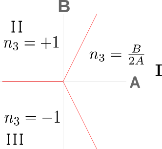
Figure 1: The three ferromagnetic phases of the potential $U(n_{3})=-Bn_{3}+An_{3}^{2}$.

Our field equations admit not only one-dimensionally modulated solutions but also homogeneous configurations as solutions.

They are the ground states in parameter regions with vanishing or small DM term. Homogeneous solutions are given by the stationary points of the potential, and are in common with the model in two or higher spatial dimensions which has the same potential as in Eq. (2), see for instance Refs. BRS ; RSN .

Restricting to homogeneous solutions and comparing the energy density results in the familiar phase diagram shown in Fig. 1.

There are three distinct regions:

1. region I: $-2A\leq B\leq 2A$, with the minimum at $n_{3}=\frac{B}{2A}$, and

   $${\cal E}_{\rm canted}=U_{\rm min}=-\frac{B^{2}}{4A}.$$ (10)

   This is the canted ferromagnetic phase. The minimum configuration of $\vec{n}$ is the circle $(n_{1})^{2}+(n_{2})^{2}=1-\frac{B^{2}}{4A^{2}}$.

2. region II: $B\geq 0$, and $B\geq 2A$, with minimum at $n_{3}=1$, and

   $${\cal E}_{+}=U_{\rm min}=A-B.$$ (11)

   This is the positively polarized ferromagnetic phase.

3. region III: $B\leq 0$, and $B\leq 2A$, with the minimum of the potential

   $${\cal E}_{-}=U_{\rm min}=A+B,$$ (12)

   at $n_{3}=-1$. This is the negatively polarized ferromagnetic phase.

The phase boundary lines are located at $B=2A\geq 0$ (between I and II), $B=0,A\leq 0$ (between II and III), and $B=2A\leq 0$ (between II and III). The order of the phase transition was found previously Hongo:2019nfr .

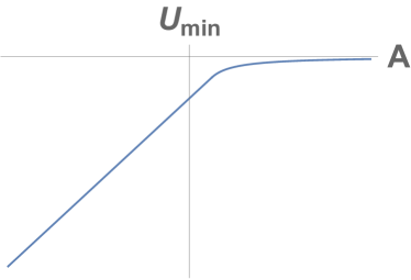
Figure 2: The energy density $\mathcal{E}(A,B)=U_{\rm min}$ of the homogeneous ground state as a function of $A$ for a fixed $B\not=0$. It exhibit the second order transition between polarized ($2A<|B|$) and the canted ($|B|<2A$) ferromagnetic phase.

The phase transition between regions I and II is of second order, since the energy density and its first derivative are continuous, while the second derivative is discontinuous. Similarly the phase transition between regions I and III is also of second order. In Fig. 2, we illustrate the second order phase transition between II and I ($B>0$) or III and I ($B<0$). The phase transition between the regions II and III across the line $B=0,A<0$ is of first order, since the energy density is identical on both sides but its first derivative is discontinuous . Moreover, there are two distinct minima at $n_{3}=1$ and $n_{3}=-1$ with the same energy. In Fig. 3, we illustrate the first order phase transition between II and III (for a fixed $A<0$) in the left panel and the second order phase transition between II and I, and one between I and III (for a fixed $A>0$) in the right panel.

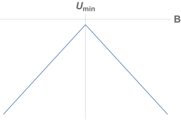
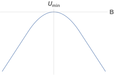
Figure 3: The energy density $\mathcal{E}(A,B)=U_{\rm min}$ of the homogeneous ground state as a function of $B$ for fixed $A$. The left panel is for fixed $A<0$, exhibiting the first order phase transition between region II and III. The right panel is for $A>0$, exhibiting the second order phase transitions between regions II (positively polarized) and I (canted), and I and III (negatively polarized) phases.

One can expect that homogeneous configurations tend to have lower energy when the potential term $U$ is more important than other terms, in particular the DM term. It is known that spiral solutions become the ground states for parameter regions where the DM interaction is more important than the potential. We will determine the precise phase boundary.

3 The field equation

3.1 Conservation of “mechanical energy”

To find the solutions for the energy density in Eq. (1), it is easiest to first solve the constraint, $(\vec{n}^{\alpha})^{2}=1$, using the independent angular variables $\Theta,\Phi$

$$\vec{n}^{\alpha}=(\sin\Theta\cos\Phi,\sin\Theta\sin\Phi,\cos\Theta)^{T}.$$ (13)

The energy density in Eq. (1) is given in terms of the independent fields $\Theta(x)$ and $\Phi(x)$ as

$$\begin{split}\mathcal{E}&=\frac{1}{2}\left\{\left(\frac{d\Theta}{dx}\right)^{2}+\left(\sin\Theta\frac{d\Phi}{dx}\right)^{2}\right\}+\kappa\left(\sin\Phi\frac{d\Theta}{dx}+\frac{1}{2}\sin 2\Theta\frac{d}{dx}\sin\Phi\right)+U(\Theta),\end{split}$$ (14)

with the potential

$$U(\Theta)=-B\cos\Theta+A\cos^{2}\Theta.$$ (15)

Minimising the energy functional leads to the Euler-Lagrange or field equations for $\Theta$ and $\Phi$ being

$$-\frac{d^{2}\Theta}{dx^{2}}+\frac{1}{2}\sin 2\Theta\left(\frac{d\Phi}{dx}\right)^{2}-2\kappa\sin^{2}\Theta\frac{d\sin\Phi}{dx}+\frac{\partial U}{\partial\Theta}=0,$$ (16)

$$-\frac{d}{dx}\left(\sin^{2}\Theta\frac{d\Phi}{dx}\right)+2\kappa\sin^{2}\Theta\cos\Phi\frac{d\Theta}{dx}=0.$$ (17)

These equations are written down for the case $B=0$ and $\alpha=\frac{3\pi}{2}$ in Chovan , where they are numerically studied, including beyond the constant $\Phi$ approximation that we make here. It is worth reiterating here that the flat spirals we consider here have $\Phi(x)=$ constant, while a non-flat spiral would not have this restriction.

As a first step, we solve Eq. (17) for $\Phi(x)$ by assuming a constant value. We then find

$$\Phi(x)=\left(2n\pm\frac{1}{2}\right)\pi,\quad n\in\mathbb{Z}.$$ (18)

Then the DM interaction term $\kappa$ disappears from the field equation for $\Theta(x)$ and Eq. (16) becomes

$$\frac{d^{2}\Theta}{dx^{2}}=+\frac{\partial U}{\partial\Theta}.$$ (19)

If we regard $x$ as “time”, Eq. (19) is the equation of motion of a particle with unit mass moving in the periodic potential $-U(\Theta)$. Since the potential is periodic, the particle is constrained to move on a circle, $S^{1}$. This classical mechanics analogy is useful for classifying solutions and finding their properties. Multiplication of (19) by $\frac{d\Theta}{dx}$ gives a conservation law corresponding to translational invariance

$$\frac{1}{2}\left(\frac{d\Theta}{dx}\right)^{2}-U(\Theta)=C_{0},$$ (20)

where the constant $C_{0}$ is a conserved quantity (an integral of motion) corresponding to the “mechanical energy” (sum of kinetic and “potential energy” $-U(\Theta)$) in classical mechanics.

3.2 Classification of solutions

We denote the value of the maximum of the potential as $U_{\rm max}$.

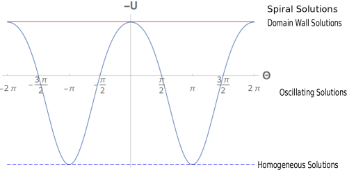
Figure 4: A plot of the potential $-U_{\rm min}(\Theta)$ for the “mechanical analog” when $B>2A$. The upper solid horizontal line (red) is $-U_{\rm min}=-A+B$ and the lower horizontal dashed line (blue) is $-U_{\rm max}$. Motions (from right to left) with the “mechanical energy” $C_{0}>-U_{\rm min}$ give spiral solutions. Motions with $C_{0}=-U_{\rm min}$ connect two neighboring $\Theta_{\rm min}$ and give domain wall solutions. Motions with $C_{0}<-U_{\rm min}$ give oscillating solutions.

Since a symmetry $B\to-B,n_{3}\to-n_{3}$ allows us to obtain solutions for $B\leq 0$ from those of $B\geq 0$, we concentrate here on regions I and II. The conservation law implies that solutions exist if and only if $C_{0}\geq-U_{\rm max}$, because of the positivity $(\frac{d\Theta}{dx})^{2}\geq 0$. We depict a typical figure of $-U(\Theta)$ for the region II in Fig. 4. In the captions we discuss the qualitatively different types of solutions in terms of the value of $C_{0}$.

Using the constant solution (18) for $\Phi$, the energy density becomes

$$\mathcal{E}_{\rm sol}=\kappa\frac{d\Theta}{dx}+\frac{1}{2}\left(\frac{d\Theta}{dx}\right)^{2}+U(\Theta).$$ (21)

The energy of the solution depends on the DM interaction term, even though the field equation (19) does not. However, the DM term does not contribute to the energy for homogeneous oscillating solutions after averaging over one period.

The inequality $\frac{1}{2}\left(\frac{d\Theta}{dx}\right)^{2}+U(\Theta)\geq U_{\rm min}$ implies that the energy density of the homogeneous ground state at $\Theta_{\rm min}$ is lower than the average energy densities of the oscillating solutions and other homogeneous solutions. We will study spiral solutions and domain wall solutions in order to find the ground state of a one dimensional chiral magnet in the following.

For the spiral and domain wall solutions with $C_{0}>-U_{\rm min}$, Eq. (20) implies that $\frac{d\Theta}{dx}$ never vanishes. Hence its sign never changes, and the solutions are monotonic. Since the energy density (21) favors the negative sign for $\frac{d\Theta}{dx}$, we should choose the negative chirality solution with $\frac{d\Theta}{dx}<0$ in order to obtain the ground state of the chiral magnet. Therefore we need to solve the following first order equation

$$\frac{d\Theta}{dx}=-\sqrt{2(C_{0}+U(\Theta))}.$$ (22)

By making use of the conservation of “mechanical energy” from Eq. (20), we can rewrite the energy density as

$$\mathcal{E}_{\rm sol}=\kappa\frac{d\Theta}{dx}+\left(\frac{d\Theta}{dx}\right)^{2}-C_{0}=\kappa\frac{d\Theta}{dx}+2U(\Theta)+C_{0}.$$ (23)

Explicit solutions are found by integrating the first order equation (22). We observe that the solutions are given in terms of elliptic functions. In the next subsection, however, we derive general properties of spiral solutions and will calculate the phase boundary between the spiral and homogeneous phases without needing to find explicit solutions.

4 Properties of spiral solutions

4.1 Spiral solutions without the potential

As a warm up for studying more general spirals let us first consider the case without a potential, $A=B=0,U(\Theta)=0$. This has been treated in the literature before BH and we discuss it here to set up our conventions for future sections. In this case, we need $C_{0}\geq 0$ and obtain $\frac{d\Theta}{dx}=-\sqrt{2C_{0}}$ from (22). The general solutions contain one additional parameter, $x_{0}$ as a Nambu-Goldstone (NG) mode for the spontaneously broken translational symmetry,

$$\Theta(x)=-\sqrt{2C_{0}}(x-x_{0}).$$ (24)

The magnetisation vector is $n_{3}+in_{2}^{\alpha}=e^{-i\sqrt{2C_{0}}(x-x_{0})}$ rotating along $x$ with the momentum $-\sqrt{2C_{0}}<0$, namely a negative chirality plane wave as a spiral solution. The period $L$ of this spiral solution is $L=2\pi/\sqrt{2C_{0}}$. Although all the configurations with different values of $C_{0}$ are solutions of the equations of motion, they have different energy densities

$$\mathcal{E}=-\kappa\sqrt{2C_{0}}+C_{0}.$$ (25)

As illustrated in the left panel of Fig. 5, the energy $\mathcal{E}$ of spiral solutions as a function of $C_{0}$ has a minimum at $C_{0,{\rm min}}=\frac{\kappa^{2}}{2}$ giving the lowest energy spiral solution as

$$\mathcal{E}_{\rm min}=-C_{0,{\rm min}}=-\frac{\kappa^{2}}{2}.$$ (26)

This energy density is lower than that of the homogeneous solution ($\mathcal{E}_{\rm homogeneous}=0$), thus $A=B=0$ is in the spiral phase. For later use, we define the excess energy $f(C_{0};A=B=0)$ in one period above the constant energy density $-C_{0}$ as

$$f(C_{0};A=B=0)=\int_{0}^{L}dx(\mathcal{E}+C_{0})=-2\pi\kappa+2\pi\sqrt{2C_{0}}.$$ (27)

As illustrated in the right panel of Fig. 5, $f(C_{0};A=B=0)$ increases monotonically and vanishes at $C_{0}=C_{0,{\rm min}}=\frac{\kappa^{2}}{2}$.

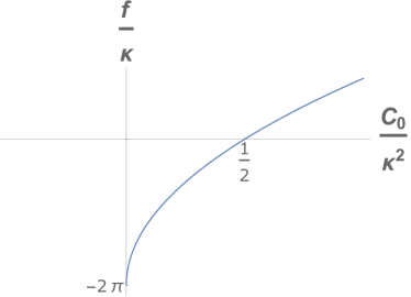
Figure 5: Left: Energy density $\mathcal{E}$ of spiral solutions as a function of $C_{0}$ for $A=B=0$. The lowest energy spiral solution occurs at $C_{0}=C_{0,{\rm min}}=\kappa^{2}/2$, giving the energy density $\mathcal{E}_{\rm min}=-\kappa^{2}/2$ for the spiral ground state. Right: The excess energy $f(C_{0};A=B=0)$ in one period as a function of $C_{0}$ for $A=B=0$. It increases monotonically and vanishes at $C_{0}=C_{0,{\rm min}}=\kappa^{2}/2$.

4.2 Lowest energy flat spiral solution

Although spiral solutions (including domain wall solutions) are monotonic functions of $\Theta$, they are periodic as a function of magnetization vector $\vec{n}$. We define the period $L$ of spiral solutions as the distance corresponding to translation by $2\pi$ in $\Theta$. Since Eq. (22) gives a one-to-one correspondence between $x$ and $\Theta$, once the NG mode $x_{0}$ is fixed by $\Theta(x_{0})=0$ for instance. We can now change variable from $x$ to $\Theta$ by using Eq. (22). The period $L$ of a spiral solution is given by

$$L=\int_{0}^{L}dx=\int_{0}^{2\pi}d\Theta\left[-\frac{d\Theta}{dx}\right]^{-1}=\int_{0}^{2\pi}\frac{d\Theta}{\sqrt{2(C_{0}+U(\Theta))}}.$$ (28)

The average energy density $\langle\mathcal{E}\rangle$ is given by

$$\langle\mathcal{E}\rangle=\frac{1}{L}\int_{0}^{L}dx\,\mathcal{E}=\frac{f(C_{0};A,B)}{L}-C_{0},$$ (29)

where

$$\begin{split}f(C_{0};A,B)&=\int_{0}^{L}dx\left[\kappa\frac{d\Theta}{dx}+\left(\frac{d\Theta}{dx}\right)^{2}\right]\\ &=-2\pi\kappa+\int_{0}^{2\pi}d\Theta\sqrt{2(C_{0}+U(\Theta))},\end{split}$$ (30)

is the energy in one period due to the excess energy density above the constant value $-C_{0}$. As in Eq. (27) we call $f(C_{0};A,B)$ the excess energy. Only the first term of the excess energy comes from the DM interaction, this gives a negative energy contribution only when the solution has a non-zero winding ($-2\pi$) after one period of translation. This feature makes it a possibility for spiral solutions to have lower average energy density than the homogeneous ground state.

For fixed values of parameters $\kappa,A,B$, our spiral solutions have two parameters (moduli) $C_{0}$ and $x_{0}$. The average energy density depends only on $C_{0}$ and is independent of $x_{0}$. Therefore we need to look for the lowest energy solution among spiral solutions, by minimizing the average energy density as a function of $C_{0}$. We find the identities

$$\frac{\partial f(C_{0};A,B)}{\partial C_{0}}=\int_{0}^{2\pi}\frac{d\Theta}{\sqrt{2(C_{0}+U(\Theta))}}=L,$$ (31)

$$\frac{\partial L}{\partial C_{0}}=-\int_{0}^{2\pi}\frac{d\Theta}{(2(C_{0}+U(\Theta)))^{3/2}},$$ (32)

some of which are also given in Chovan . Thus we obtain

$$\frac{\partial\langle\mathcal{E}\rangle}{\partial C_{0}}=\frac{-1}{L^{2}}\frac{\partial L}{\partial C_{0}}f(C_{0};A,B).$$ (33)

Eq. (31) shows that $f(C_{0};A,B)$ is monotonically increasing. Because of (32), the average energy density reaches a minimum when

$$f(C_{0};A,B)=-2\pi\kappa+\int_{0}^{2\pi}d\Theta\sqrt{2(C_{0}+U(\Theta))}=0,$$ (34)

is satisfied, provided this value of $C_{0,{\rm min}}$ is in the allowed region of spiral solutions $C_{0}\geq-U_{\rm min}$. This minimum energy condition (34) gives $C_{0,{\rm min}}$ as a function of $A$ and $B$. Eq. (29) implies that the average energy density of the lowest energy spiral solution is given by this $C_{0,{\rm min}}$ as

$$\langle\mathcal{E}\rangle_{\rm min}=-C_{0,{\rm min}}.$$ (35)

Hence the lowest energy spiral solution always has lower energy than the homogeneous ground state with the energy density $U_{\min}$

$$\langle\mathcal{E}\rangle_{\rm min}=-C_{0,{\rm min}}\leq U_{\rm min}.$$ (36)

We conclude that a chiral magnet is in the spiral phase, once the minimum energy condition is satisfied in the allowed region for spiral solutions $C_{0}>-U_{\rm min}$.

4.3 Boundary between spiral and homogeneous phases

As given in Eq. (27), the function $f$ at $A=B=0$ becomes $f(C_{0};A=B=0)=-2\pi\kappa+2\pi\sqrt{2C_{0}}$. This behaves asymptotically as $f(C_{0};A=B=0)\sim 2\pi\sqrt{2C_{0}}>0$ for $C_{0}\to\infty$ whereas $f(C_{0}=-U_{\rm min}=0;A=B=0)=-2\pi\kappa^{2}<0$. Hence the excess energy $f(C_{0};A=B=0)$ has a zero in the region $C_{0}>-U_{\rm min}$, ensuring the existence of the lowest energy spiral solution for $A=B=0$.

Let us now study the case of nonvanishing values of $A,B$, such that $2A\leq B$. We observe that the excess energy $f(C_{0};A,B)$ at $C_{0}\gg A,B,\kappa^{2}$ becomes asymptotically

$$f(C_{0};A,B)\sim 2\pi\sqrt{2C_{0}}>0.$$ (37)

Since the excess energy $f(C_{0};,B)$ is monotonically increasing, the zero of the excess energy $f(C_{0};A,B)=0$ occurs in the allowed region if and only if $f(C_{0}=-U_{\rm min};A,B)<0$.

When $C_{0}$ approaches the lower bound at $-U_{\rm min}$, we find

$$L\to\infty,$$ (38)

since the integrand diverges at $\Theta=\Theta_{\rm min}$, as $\sqrt{C_{0}+U(\Theta)}\to\sqrt{\frac{U^{\prime\prime}(\Theta_{\rm min})}{2}}|\Theta-\Theta_{\rm min}|$ with $U^{\prime\prime}=\frac{d^{2}U}{d\Theta^{2}}$. On the other hand, the excess energy remains finite as $C_{0}\to-U_{\rm min}$. Therefore the average energy density (29) becomes

$$\left.\langle\mathcal{E}\rangle\right|_{C_{0}=-U_{\rm min}}=U_{\rm min},$$ (39)

which is the same as that of the homogeneous solution. We denote the excess energy at this $C_{0}=-U_{\rm min}$ as

$$E_{\rm period}(A,B) =f(C_{0}=-U_{\rm min};A,B)$$

$$=-2\pi\kappa+\int_{0}^{2\pi}d\Theta\sqrt{2(U(\Theta)-U_{\rm min})}.$$ (40)

Summarizing the above, we find that the chiral magnet is in the spiral phase if
$E_{\rm period}(A,B)<0$, and in the homogeneous phase if $E_{\rm period}(A,B)>0$. The phase boundary between spiral phase and the homogeneous phases is given by

$$0=E_{\rm period}(A,B)=-2\pi\kappa+\int_{0}^{2\pi}d\Theta\sqrt{2(U(\Theta)-U_{\rm min})}.$$ (41)

Since the period is infinite, the spiral solution in this limit becomes a domain wall solution connecting two adjacent values of $\Theta_{\min}$. We will describe more explicitly the domain wall solutions as a limit of spiral solutions in a later section. Since $-U_{\rm min}$ is the energy density of the homogeneous solution, the excess energy above this energy density integrated over one period $E_{\rm period}(A,B)$ is precisely the domain wall energy as a finite energy soliton solution on the homogeneous background. Our results show that the domain wall solution as a single soliton above the homogeneous background has positive energy and is an ordinary excitation in the homogeneous phase. It becomes zero energy at the boundary between the homogeneous and spiral phases. It has a negative energy in the spiral phase region, and signals the instability of the homogeneous background solution and its decay to the lowest energy spiral solution as the true ground state. One can intuitively visualize the deformation of the configuration as a condensation of these negative energy solitons settling down to the spiral ground state.

4.4 Explicit formula for phase boundaries

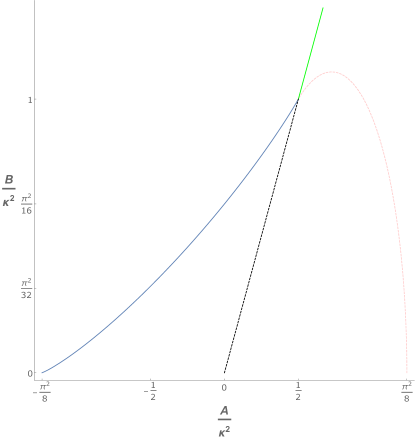
Figure 6: The phase diagram in the $\frac{A}{\kappa^{2}},\frac{B}{\kappa^{2}}$ plane. The spiral phase is below the blue curve. The(positively) polarized ferromagnetic phase is above the blue curve. The two ferromagnetic phases are separated by the green line $B=2A$. Below the tricritical point $B=2A=\kappa^{2}$, the dashed line $B=2A$ does not correspond to a phase boundary. The dashed red line shows where flat spirals in the anisotropy dominated case have zero energy. This is not a phase boundary as the flat spiral is not the ground state.

When $2A\leq B$, the homogeneous phase in this region is the polarized ferromagnetic phase $n_{3}=+1$. The minimum of the potential is $U_{\rm min}=A-B$ which occurs at $\Theta_{\rm min}=2{\mathbb{Z}}\pi$. We find that the boundary in Eq. (41) between the polarized ferromagnetic phase and the spiral phase is given by

$$2\pi\kappa =\int_{0}^{2\pi}d\Theta\sqrt{2(-B\cos\Theta+A\cos^{2}\Theta-A+B)}$$

$$=4\sqrt{B-2A}+\frac{4B}{\sqrt{2A}}\arcsin\sqrt{\frac{2A}{B}}.$$ (42)

This boundary is depicted as the (blue) curve to the left of $B=2A$ line in Fig. 6. This expression is manifestly real for $0\leq A$. This formula is also valid for $A\leq 0$ by an analytic continuation of $A>0\to A<0$. We find a convenient (manifestly real) expression in the region $A\leq 0$ to be

$$2\pi\kappa =4\sqrt{B-2A}+\frac{4B}{\sqrt{-2A}}\operatorname{arcsinh}\sqrt{\frac{-2A}{B}}$$ (43)

$$=4\sqrt{B-2A}+\frac{2B}{\sqrt{-2A}}\log\left(\frac{\sqrt{B-2A}+\sqrt{-2A}}{\sqrt{B-2A}-\sqrt{-2A}}\right),$$

where the last expression agrees with the one derived in the case of $A\leq 0$ previously BH , apart from the difference in conventions.

This boundary curve is also depicted as the (blue) curve to the left of the $B=2A$ line in Fig. 6.

For completeness, in order to see the region of negative $B$, we note that the phase diagram is symmetric under $B\to-B$.

Although partial results for particular parameter values or regions have been obtained for the phase boundary between homogeneous ferromagnetic phases and spiral phase, our results give the complete boundary curve explicitly for the first time.

4.5 Order of phase transition between spiral and homogeneous phases

In this subsection, we will demonstrate that the phase transition between the spiral and homogeneous phases is of second order.

The phase transition is of the $n$-th order if the $l$-th order derivatives of the free energy at the phase boundary are continuous for $l<n$ and discontinuous for $l=n$. At zero temperature, the free energy density is given by the average energy density of the ground state. In the homogeneous phase, the energy density is given by the minimum $U_{\rm min}$ of the potential. The average energy density of spiral phase $\langle\mathcal{E}\rangle_{\rm spiral}$ is given by that of the lowest energy spiral solution in Eq. (35)

$$\langle\mathcal{E}\rangle_{\rm spiral}=-C_{0,{\rm min}}(A,B),$$ (44)

where the mechanical energy $C_{0,{\rm min}}$ of the lowest energy spiral solution is determined as a function of the potential parameters $A,B$ by the minimum energy condition in Eq. (34) as

$$2\pi\kappa =\int_{0}^{2\pi}d\Theta\sqrt{2(U(\Theta)+C_{0,{\rm min}})}$$

$$=\int_{0}^{2\pi}d\Theta\sqrt{2(-B\cos\Theta+A\cos^{2}\Theta+C_{0,{\rm min}})}.$$ (45)

As noted in Eq. (39), the energy density of the spiral phase tends continuously to that of the homogeneous phase at the phase boundary

$$\langle\mathcal{E}\rangle_{\rm spiral}\to U_{\rm min}(A,B)=\langle\mathcal{E}\rangle_{\rm homogeneous}.$$ (46)

Since the energy density along the boundary is common for homogeneous and spiral phases, all of their derivatives tangential to the phase boundary are continuous between the homogeneous and spiral phases. Therefore, we need to consider only the derivative perpendicular to the boundary.

Let us parametrize the difference between the energy density of the spiral and homogeneous phases in terms of the deviation $\Delta C\geq 0$ defined as

$$C_{0,{\rm min}}(A,B)=-U_{\rm min}(A,B)+\Delta C(A,B),$$ (47)

$$\langle\mathcal{E}\rangle_{\rm spiral}-\langle\mathcal{E}\rangle_{\rm homogeneous}=-\Delta C(A,B).$$ (48)

The limiting procedure of the parameters $A,B$ approaching the phase boundary is equivalent to $\Delta C(A,B)\to 0$. We can obtain the first derivative of $\Delta C$ in terms of $A,B$ by differentiating the minimum energy condition in Eq. (45)

$$0=\int_{0}^{2\pi}d\Theta\frac{-\frac{\partial U_{\rm min}}{\partial A}+\frac{\partial\Delta C}{\partial A}+\cos^{2}\Theta}{\sqrt{2(U(\Theta)-U_{\rm min}+\Delta C)}},$$ (49)

$$0=\int_{0}^{2\pi}d\Theta\frac{-\frac{\partial U_{\rm min}}{\partial B}+\frac{\partial\Delta C}{\partial B}-\cos\Theta}{\sqrt{2(U(\Theta)-U_{\rm min}+\Delta C)}}.$$ (50)

We can rewrite these relations as

$$-\frac{\partial\Delta C}{\partial A}=\frac{L_{0}^{01}}{L},\quad-\frac{\partial\Delta C}{\partial B}=\frac{L_{0}^{10}}{L},$$ (51)

where the period $L$ and weighted integrals $L_{n}^{kl}$ are defined as

$$L=L_{0}^{00}=\int_{0}^{2\pi}\frac{d\Theta}{\sqrt{2(U(\Theta)-U_{\rm min}+\Delta C)}},$$ (52)

and

$$L_{n}^{kl}=\int_{0}^{2\pi}d\Theta\frac{\left(-\frac{\partial U_{\rm min}}{\partial B}-\cos\Theta\right)^{k}\left(\cos^{2}\Theta-\frac{\partial U_{\rm min}}{\partial A}\right)^{l}}{[2(U(\Theta)-U_{\rm min}+\Delta C)]^{n+1/2}}.$$ (53)

As is derived in Appendix A, $L\to\infty$ in the limit of $\Delta C\to 0$, whereas $L_{0}^{10},L_{0}^{01}$ are finite. Therefore, we obtain at the phase boundary

$$\frac{\partial\Delta C}{\partial A}\to 0,\quad\frac{\partial\Delta C}{\partial B}\to 0,$$ (54)

implying that the first derivative of energy density is continuous at the phase boundary.

Similarly we can obtain the second derivative of $\Delta C$ by differentiating (50) and (49) in terms of $A,B$ again. We find an exact expression for $\frac{\partial^{2}\Delta C}{\partial A_{i}\partial A_{j}}$ with $A_{1}=A,A_{2}=B$ using the integral in Eq. (53) . As described in Appendix A, we find that the second derivative diverges at the boundary

$$-\left(\begin{array}[]{cc}\frac{\partial^{2}\Delta C}{\partial A^{2}}&\frac{\partial^{2}\Delta C}{\partial A\partial B}\\ \frac{\partial^{2}\Delta C}{\partial B\partial A}&\frac{\partial^{2}\Delta C}{\partial B^{2}}\end{array}\right)\sim-\frac{L_{1}^{00}}{L^{3}}\left[\left(\begin{array}[]{c}L_{0}^{01}\\ L_{0}^{10}\end{array}\right)\left(\begin{array}[]{cc}L_{0}^{01}&L_{0}^{10}\end{array}\right)\right]_{\rm boundary},$$ (55)

with the asymptotic behavior as $\Delta C\to 0$

$$\frac{L_{1}^{00}}{L^{3}}\sim\frac{1}{\Delta C\left(\log\frac{1}{\Delta C}\right)^{3}}\to+\infty.$$ (56)

Therefore the second derivative of the difference of energy density $\langle\mathcal{E}\rangle_{\rm spiral}-\langle\mathcal{E}\rangle_{\rm homogeneous}=-\Delta C$ is not continuous. Hence we conclude that the phase transition between homogeneous phases and the spiral phase is of second order.

The rank of the coefficient matrix is unity. This corresponds to the fact that the derivative is nonzero only along the normal to the phase boundary. The boundary is defined by Eq. (41) corresponding to $\Delta C=0$. By varying this condition we find that along the boundary

$$0=\frac{dA}{dB}\left[L_{1}^{01}\right]_{\rm boundary}+\left[L_{0}^{10}\right]_{\rm boundary}.$$ (57)

The relation shows that the second derivative vanishes along the tangential direction to the boundary.

4.6 Exact spiral solutions

As we have seen in the previous sections, there is a spiral phase in the regions below the boundary line defined in Eq. (41). In order to illustrate our results more explicitly, we here present exact spiral solutions for the simple typical cases. The solutions are given in terms of elliptic functions and the technical details are relegated to Appendix B.1. Here we just present the period and energy of the solutions. Throughout this section $K(k)$ and $E(k)$ are the complete elliptic integral of the first and the second kind defined as

$$K(k) =\int_{0}^{\frac{\pi}{2}}\frac{d\varphi}{\sqrt{1-k^{2}\sin^{2}\varphi}},$$ (58)

$$E(k) =\int_{0}^{\frac{\pi}{2}}d\varphi\sqrt{1-k^{2}\sin^{2}\varphi},$$ (59)

respectively.

4.6.1 Spirals without external magnetic fields ($B=0$)

In the case of nonzero anisotropy ($A\not=0$) without the Zeeman term ($B=0$), the first order equation for $\Theta(x)$ in Eq. (22) becomes

$$\frac{d\Theta}{dx}=-\sqrt{2(C_{0}+A\cos^{2}\Theta)}.$$ (60)

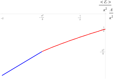
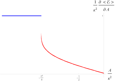
Figure 7: Case of $B=0$. Red solid curves and blue solid curves correspond to spiral phase and homogeneous ferromagnetic phase, respectively. Left: Average energy density $\langle\mathcal{E}\rangle_{min}=-C_{0}(A,0)$ as a function of $\frac{A}{\kappa^{2}}$, determined by Eqs. (61), (63), and (64) for $A<0$. Right: Derivative of average energy density as a function of $\frac{A}{\kappa^{2}}$. The second derivative diverges at the phase boundary $A=-\frac{(\pi\kappa)^{2}}{8}$ showing the second order phase transition.

$A<0$ case:

The elliptic modulus $k$ and the period $L$ in this case are given by

$$k=\sqrt{\frac{-A}{C_{0}}},\quad L=\frac{4}{\sqrt{2C_{0}}}K(k).$$ (61)

The average energy density of the spiral solution $\langle\mathcal{E}\rangle=\frac{f(C_{0};A>0,B=0)}{L}-C_{0}$ is minimized by the condition of vanishing excess energy

$$f(C_{0};A<0,B=0)=-2\pi\kappa+4\sqrt{2C_{0}}E(k)=0,$$ (62)

which determines $C_{0}(A)$ as a function of $A$ through

$$A=-\frac{\pi^{2}\kappa^{2}}{8}\left(\frac{k}{E(k)}\right)^{2}.$$ (63)

and (61). The minimum energy density

$$\langle\mathcal{E}\rangle=-C_{0}(A).$$ (64)

The critical point occurs at $A=-\frac{\pi^{2}}{8}$. At this point, the energy density of the lowest energy spiral solution becomes equal to that of the ferromagnetic state.

The average energy density of the lowest energy spiral solutions and its derivatives are plotted in Fig. 7 exhibiting the second order phase transitions at $A=\pm\frac{\pi^{2}\kappa^{2}}{8}$.

4.6.2 Spiral solutions without anisotropy ($A=0$)

The solution for $A=0$ has been studied previously KO2015 . In this case the first order equation for $\Theta(x)$ in Eq. (22) becomes

$$\frac{d\Theta}{dx}=-\sqrt{2(C_{0}-B\cos\Theta)}.$$ (65)

The solutions are elliptic functions with the elliptic modulus $k$ and the period $L$

$$k=\sqrt{\frac{2B}{C_{0}+B}},\quad L=2\sqrt{\frac{2}{C_{0}+B}}K(k).$$ (66)

The average energy density of the spiral solution $\langle\mathcal{E}\rangle=\frac{f(C_{0};A>0,B=0)}{L}-C_{0}$ is minimized by the condition of vanishing excess energy

$$f(C_{0};A=0,B)=-2\pi\kappa+4\sqrt{2(C_{0}+B)}E(k),$$ (67)

which determines $C_{0}(B)$ as a function of $B$ through

$$B=\frac{\pi^{2}\kappa^{2}}{16}\left(\frac{k}{E(k)}\right)^{2},$$ (68)

and (66). The minimum energy density is given by

$$\langle\mathcal{E}\rangle=-C_{0}(B),$$ (69)

where $C_{0}(B)$ is defined by (67). This energy density $-C_{0}(B)\leq 0$ is lower than the energy density of the positively polarized ferromagnetic state with the energy density $-B$. As $C_{0}$ approaches the lowest allowed value $-U_{\rm min}=B$, the period $L$ becomes infinite, and the lowest energy spiral solution has the same average energy density as the ferromagnetic state. This critical point $B=\frac{\pi^{2}}{16}\kappa^{2}$ occurs at the $C_{0}\to 0$ limit of the minimum energy condition (67).

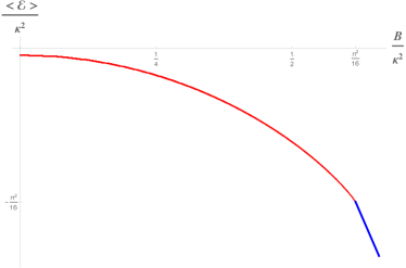
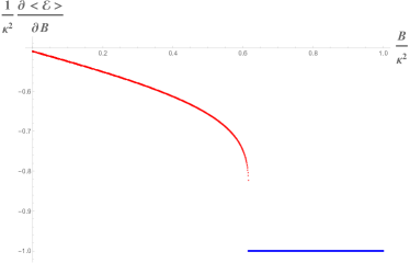
Figure 8: Case of $A=0$. Red solid curves and blue solid curves correspond to spiral phase and homogeneous ferromagnetic phase, respectively. Left: Average energy density $\langle\mathcal{E}\rangle_{min}=-C_{0}(A=0,B)$ as a function of $\frac{B}{\kappa^{2}}$, determined by Eqs. (66), (68), and (69). Right: Derivative of average energy density as a function of $\frac{B}{\kappa^{2}}$. The second derivative diverges at the phase boundary $B=\frac{(\pi\kappa)^{2}}{16}$ showing the second order phase transition.

As an example we draw the energy density, its first and second derivatives as a function of $A$ in the case of $B=0$ in Fig. 7. Similar plots of the energy density, and its first and second derivatives are given as a function of $B$ for the case of $A=0$ in Fig. 8.

4.7 Domain walls as infinite period limit of spirals

For generic values of parameters $A,B$, one can still integrate (22), since it is an elliptic integral. We can express the one-to-one mapping between $x$ and $\Theta$ of spiral solutions in terms of Jacobi elliptic functions, although the mapping is similar to, but algebraically more involved than the explicit spiral solutions in simple cases: Eq. (117) in the case of $A=0$, and Eq. (111) in the case of $B=0,A<0$. One should note that the functional form of the profile function $\Theta(x)$ of the domain wall solutions or spiral solutions are determined solely by the parameters of the potential $A,B$ and $C_{0}$, but are independent of the DM interaction parameter $\kappa$. The DM interaction parameter comes in only when we evaluate the average energy density of the spiral solutions or domain wall solutions. Therefore the lowest energy spiral solutions and the critical point explicitly depends on the DM parameter $\kappa$. Similarly the domain wall solutions can exist irrespective of the value of $\kappa$, but they become zero energy solitons at the phase boundary between spiral and homogeneous ferromagnetic phases.

Let us examine the infinite period limit of the lowest energy spiral solutions. As we approach the phase boundary, the period of spiral solutions tends to infinity, and the solutions become domain wall solutions, as we argued. At the boundary we find the average energy density becomes identical to that of the homogeneous solution. Moreover, the total energy of the domain wall vanishes at the boundary. We will explicitly see these properties by studying domain wall solutions in all parameter regions across the phase boundary in the following section. The domain wall solutions $\Theta(x)$ can be expressed in terms of elementary functions. This corresponds to the fact that the elliptic function describing a spiral solution becomes an elementary function in the limit of infinite period. Let us take the limit of infinite period for illustrative examples of spiral solutions in the case of $A=0$ and $B=0$.

Figure 9: This is the profile function $\Theta$ from Eq. (70) plotted against the dimensionless variable $\kappa x$ for the critical value $\frac{B}{\kappa^{2}}=\frac{\pi^{2}}{16}$ at $A=0$.

$A=0,B>0$ Case :

One period of the spiral solution (117) reduces to two sets of the following domain wall solution in the limit of infinite period $k\to 1$ corresponding to $B=\frac{(\pi\kappa)^{2}}{16}$

$$\begin{split}\Theta&=-4\arctan\left(\exp(\sqrt{B}x)\right),\\ \vec{n}^{\alpha}&=\left(0,2\frac{\tanh\left(\sqrt{B}x\right)}{\cosh\left(\sqrt{B}x\right)},1-2\operatorname{sech}^{2}\left(\sqrt{B}x\right)\right)^{T}.\end{split}$$ (70)

We note that this is a domain wall solution for any $B>0$ with $A=0$. The total energy of the domain wall is zero at the phase transition point $B=\frac{(\pi\kappa)^{2}}{16}$, positive in the positively polarized ferromagnetic phase $B>\frac{(\pi\kappa)^{2}}{16}$, and negative in the spiral phase $B<\frac{(\pi\kappa)^{2}}{16}$. We plot this on the right in Fig. 9. It should be noted that while we have referred to the configurations as domain walls for $A=0,B>0$ they do not connect two different magnetic domains. In fact they interpolate between a magnetic domain and itself, since their phase rotates by a full $2\pi$. Some times these configurations would be called kinks, however, we would reserve that for when they are genuine soliton solutions with positive energy above the ferromagnetic phase. As such we stick to calling them domain walls.

5 Domain walls in chiral magnets

5.1 Exact domain wall solutions

Since the field equation (19) involves only the potential parameters $A,B$ and is independent of the DM interaction parameter $\kappa$, the shapes of domain wall solutions are identical to those of the double sine-Gordon model. For instance, Ref. Condat1983 gave domain wall solutions for the double sine-Gordon model, but in an entirely different physical context. The functional form of our exact solutions agree with those in Ref. Condat1983 after adjusting for the different conventions. However, our energy functional involves the DM term, which gives a crucial negative energy contribution for the energy of domain wall solution as solitons. This fact is the basis of our finding of zero energy domain wall solutions at the boundary between the homogeneous phase and the spiral phase. We will derive exact domain wall solutions and evaluate their energy, in order to be reasonably self-contained.

A domain wall is a soliton with a localized energy. We will demonstrate explicitly that it has positive energy in the homogeneous phase, negative energy in the spiral phase, and zero energy at the phase boundary. The domain wall solutions are found to correspond to the infinite period limit of the lowest energy spiral solution. These features show that domain wall solutions are solitons for excited states in the homogeneous phase, but are instability modes for the homogeneous background solution in the spiral phase. This picture agrees with the fact that the lowest energy spiral solution gives the ground state in the spiral phase region, which has lower average energy density than the homogeneous solution.

The domain wall solutions of our interest are defined as those solutions of the first order equation (22) with the mechanical energy tuned as $C_{0}=-U_{\rm min}$. The first order equation for $\Theta(x)$ in Eq. (22) becomes

$$\frac{d\Theta}{dx}=-\sqrt{2(-B\cos\Theta+A\cos^{2}\Theta+U_{\rm min})},$$ (71)

which gives a monotonically decreasing function $\Theta(x)$ connecting two adjacent minima $\Theta_{\rm min}$ of the potential.

5.2 Domain wall solutions for $0\leq B\leq 2A$

In the parameter region $0\leq B\leq 2A$, the minimum of the potential is $U_{\rm min}=-\frac{B^{2}}{4A}$, and the homogeneous phase is given by the canted ferromagnetic solution with $n_{3}=\frac{B}{2A}$. The first order field equation (71) becomes

$$\frac{d\Theta}{dx}=-\sqrt{2A}\left|\cos\Theta-\frac{B}{2A}\right|.$$ (72)

Since there are two degenerate minima in one period $2\pi$, we have two different types of domain walls: the long wall connecting $\Theta=2\pi-\arccos\frac{B}{2A}$ at $x=-\infty$ to $\arccos\frac{B}{2A}$ at $x=\infty$, and the short wall connecting $\Theta=\arccos\frac{B}{2A}$ at $x=-\infty$ to $-\arccos\frac{B}{2A}$ at $x=\infty$.

5.2.1 Long wall

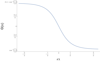
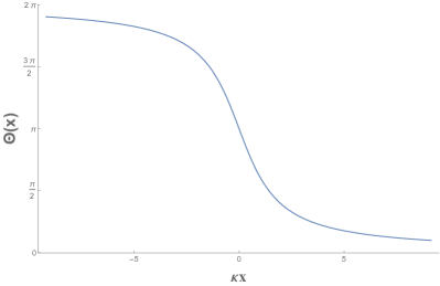
Figure 10: On the left is a plot of the profile function $\Theta$ as a function of the dimensionless quantity $\kappa x$ for the long wall for $0\leq B\leq 2A$ in Eq. (73). We take $\frac{A}{\kappa^{2}}=3,\frac{B}{\kappa^{2}}=2$ as an example, and the domain wall to be centred at $x=0$. On the right is the profile of the domain wall solution $\Theta$ and in Eq. (74) plotted against the dimensionless quantity $\kappa x$ for $B=2A=\frac{1}{2}\kappa^{2}$, with the domain wall to be centred at $x=0$.

The long wall is obtained by integrating (72) with $\frac{B}{2A}-\cos\Theta\geq 0$. By choosing $\Theta=\pi$ at $x=0$ (midpoint of the domain wall), we obtain the solution connecting $\Theta=2\pi-\arccos\frac{B}{2A}$ at $x=-\infty$ to $\arccos\frac{B}{2A}$ at $x=\infty$ as

$$x =-\frac{1}{\sqrt{2A}}\int_{\pi}^{\Theta}\frac{d\Theta^{\prime}}{\frac{B}{2A}-\cos\Theta^{\prime}}$$

$$=\sqrt{\frac{2A}{4A^{2}-B^{2}}}\log\left(\frac{\tan\frac{\Theta}{2}+\sqrt{\frac{2A-B}{2A+B}}}{\tan\frac{\Theta}{2}-\sqrt{\frac{2A-B}{2A+B}}}\right)$$

$$=\sqrt{\frac{2A}{4A^{2}-B^{2}}}\;2\;{\rm arccoth}\left(\sqrt{\frac{2A+B}{2A-B}}\tan\frac{\Theta}{2}\right).$$ (73)

On the left in Fig. 10, we plot the domain wall profile $\Theta$ as a function of $x$.

In the limit of $2A\to B+0$, the domain wall solution reduces to

$$x=\frac{1}{\sqrt{B}}\cot\frac{\Theta}{2},$$ (74)

where we choose the branch $2\pi\geq\Theta\geq\pi$ for $-\infty\leq x\leq 0$, and $\pi\geq\Theta\geq 0$ for $0\leq x\leq\infty$. This solution is depicted on the right in Fig. 10.

5.2.2 Short wall

The short wall is obtained by integrating (72) with $\cos\Theta-\frac{B}{2A}\geq 0$. By choosing $\Theta=0$ at $x=0$ (midpoint of the domain wall), we obtain the solution connecting $\Theta=\arccos\frac{B}{2A}$ at $x=-\infty$ to $-\arccos\frac{B}{2A}$ at $x=\infty$ as

$$x =-\frac{1}{\sqrt{2A}}\int_{0}^{\Theta}\frac{d\Theta^{\prime}}{\cos\Theta^{\prime}-\frac{B}{2A}}$$

$$=\sqrt{\frac{2A}{4A^{2}-B^{2}}}\log\left(\frac{\sqrt{\frac{2A-B}{2A+B}}-\tan\frac{\Theta}{2}}{\sqrt{\frac{2A-B}{2A+B}}+\tan\frac{\Theta}{2}}\right)$$

$$=-\sqrt{\frac{2A}{4A^{2}-B^{2}}}\;2\;{\rm arctanh}\left(\sqrt{\frac{2A+B}{2A-B}}\tan\frac{\Theta}{2}\right).$$ (75)

In Fig. 11, we plot the domain wall profile $\Theta$ as a function of the dimensionless quantity $\kappa x$.

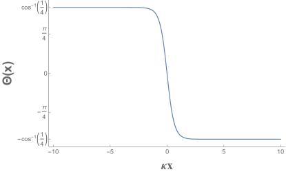
Figure 11: This is a plot of the profile function $\Theta$ as a function of the dimensionless quantity $\kappa x$ for the short wall for $0\leq B\leq 2A$ in Eq. (75). We take $\frac{A}{\kappa^{2}}=4,\frac{B}{\kappa^{2}}=2$ as an example, and the domain wall to be centered at $\kappa x=0$.

In the limit of $B\to 0$, the long wall connects $\Theta=\frac{3\pi}{2}$ to $\frac{\pi}{2}$, whereas the short wall connects $\Theta=\frac{\pi}{2}$ to $-\frac{\pi}{2}$. We find that the long and short walls at $B\to 0$ are precisely identical to those walls emerging from the infinite period limit of the spiral solution at $B=0$.

5.2.3 Energy of long and short domain walls

For the long wall, the value of $\Theta$ spans from $2\pi-\arccos\frac{B}{2A}$ at $x=-\infty$ to $\arccos\frac{B}{2A}$ at $x=\infty$. The total energy of the long domain wall on the homogeneous solution (with energy density $U_{\rm min}$) as background is given by integrating over the energy density in Eq. (23) with $C_{0}=-U_{\rm min}$:

$${E}_{\rm long} =\int_{-\infty}^{\infty}dx\left({\mathcal{E}}_{\rm sol}-U_{\rm min}\right)$$

$$=\int_{-\infty}^{\infty}dx\left(\kappa\frac{d\Theta}{dx}+2(U(\Theta)-U_{\rm min})\right).$$ (76)

Changing variable from $x$ to $\Theta$, we obtain by using the domain wall equation in Eq. (71) with $\frac{d\Theta}{dx}=-\sqrt{2(U(\Theta)-U_{\rm min})}=-\sqrt{2A}(\frac{B}{2A}-\cos\Theta)$:

$${E}_{\rm long} =\int_{2\pi-\arccos\frac{B}{2A}}^{\arccos\frac{B}{2A}}d\Theta\left(\frac{d\Theta}{dx}\right)^{-1}\left(\kappa\frac{d\Theta}{dx}+2A\left(\frac{B}{2A}-\cos\Theta\right)^{2}\right)$$ (77)

$$=-2\kappa\left(\pi-\arccos\frac{B}{2A}\right)+\frac{2B}{\sqrt{2A}}\left(\pi-\arccos\frac{B}{2A}\right)+2\sqrt{2A-\frac{B^{2}}{2A}}.$$

Similarly, the total energy of the short domain wall on the homogeneous solution as the background is given by integrating over the energy density. The only difference from the long wall is that $\Theta$ varies from $\arccos\frac{B}{2A}$ at $x=-\infty$ to $-\arccos\frac{B}{2A}$ at $x=\infty$, and $\cos\Theta-\frac{B}{2A}\geq 0$. By noting $\frac{d\Theta}{dx}=-\sqrt{2(U(\Theta)-U_{\rm min})}=-\sqrt{2A}(\cos\Theta-\frac{B}{2A})$, we find

$${E}_{\rm short} =\int_{-\arccos\frac{B}{2A}}^{\arccos\frac{B}{2A}}d\Theta\left(\frac{d\Theta}{dx}\right)^{-1}\left(\kappa\frac{d\Theta}{dx}+2A\left(\cos\Theta-\frac{B}{2A}\right)^{2}\right)$$ (78)

$$=-2\kappa\arccos\frac{B}{2A}-\frac{2B}{\sqrt{2A}}\arccos\frac{B}{2A}+2\sqrt{2A-\frac{B^{2}}{2A}}.$$

In order to obtain domain wall solutions as the infinite period limit of a spiral solution, we need to consider domain walls connecting minimum of the potential which are $\Delta\Theta=2\pi$ apart. Such limiting domain walls precisely correspond to the sum of a pair of long and short domain walls. The sum of the energy of the short and long domain wall is given by

$$E_{\rm period} ={E}_{\rm long}+E_{\rm short}$$ (79)

$$=-2\pi\kappa+\frac{4B}{\sqrt{2A}}\left(\frac{\pi}{2}-\arccos\frac{B}{2A}\right)+4\sqrt{2A-\frac{B^{2}}{2A}}.$$

Thus we see that the energy of a pair of long and short domain wall solutions is positive in the (homogeneous) ferromagnetic phase, negative in the spiral phase, and zero along the dashed red line in Fig. 6. Considering both the $B\to 2A$ and the $B\to 0$ limits of the long and short walls we see that they have the same energy in the $B\to 0$ limit, while the long wall has lower energy in the $B\to 2A$ limit. In fact for $B\to 2A$ the short domain wall disappears and has zero energy.

5.3 Domain wall solutions for $B>0$ and $B>2A$

In the parameter region $B>0$ and $B>2A$, the minimum of the potential is $U_{\rm min}=A-B$, and the homogeneous phase is given by the polarized ferromagnetic solution with $n_{3}=1$. The first order equation (71) becomes

$$\frac{d\Theta}{dx}=-\sqrt{2(1-\cos\Theta)(B-A-A\cos\Theta)}.$$ (80)

In the region $B>0$ and $B>2A$, the minimum of the potential occur at $\Theta=2\pi{\mathbb{Z}}$. Let us consider a domain wall connecting $\Theta=2\pi$ at $x=-\infty$ to $\Theta=0$ at $x=\infty$. By choosing the midpoint of the domain wall $\Theta=\pi$ at $x=0$, we find

$$x =-\int_{\pi}^{\Theta}\frac{d\Theta^{\prime}}{\sqrt{2(1-\cos\Theta^{\prime})(B-A-A\cos\Theta^{\prime})}}$$

$$=\frac{1}{\sqrt{B-2A}}\log\left(\sqrt{1+\left(1-\frac{2A}{B}\right)\cot^{2}\frac{\Theta}{2}}+\sqrt{1-\frac{2A}{B}}\cot\frac{\Theta}{2}\right).$$ (81)

In Fig. 12, we plot the domain wall profile $\Theta$ as a function of $x$. In the limit of $2A\to B-0$, the domain wall solution reduces to an identical form to the domain wall obtained in the limit of $2A\to B+0$ from Eq. (74).

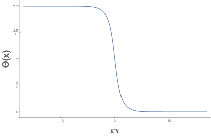
Figure 12: This is a plot of the profile function $\Theta$ as a function of the dimensionless variable $\kappa x$ for a domain wall in the magnetic field dominated region $B\geq 2A$ in Eq. (81). We take $A=\frac{\kappa^{2}}{2},B=2\kappa^{2}$ as an example, and the domain wall to be centered at $x=0$.

Since the energy density of the homogeneous solution (polarized ferromagnetic ground state) is $U_{\rm min}=A-B$, the total energy of the domain wall on the homogeneous background is given by

$${E}_{\rm DW} =\int_{-\infty}^{\infty}dx\left(\kappa\frac{d\Theta}{dx}+2(U(\Theta)-U_{\rm min})\right)$$

$$=-2\pi\kappa+4\sqrt{B-2A}+\frac{4B}{\sqrt{2A}}\arcsin\sqrt{\frac{2A}{B}},$$ (82)

in the case of $A>0$, and

$${E}_{\rm DW}=-2\pi\kappa+4\sqrt{B-2A}+\frac{4B}{\sqrt{-2A}}\operatorname{arcsinh}\sqrt{\frac{-2A}{B}},$$ (83)

in the case of $A\leq 0$. We see that the zero energy condition for the domain wall gives the boundary between the homogeneous phase and spiral phase, as given in Eqs. (42) and (43). Moreover, the domain wall is a positive energy soliton as an excited state in the homogeneous phase. In the spiral phase, on the other hand, the domain wall on the (homogeneous) ferromagnetic background solution gives a negative energy solution, signaling the instability of the ferromagnetic (homogeneous) solution. These observations confirm our conclusion that the homogeneous solution is unstable in the spiral phase and decays into the spiral solution, giving the ground state.

6 Conclusion and discussion

We have studied solutions of the field equations for chiral magnets in one spatial dimension, in order to determine their phase diagram. There are three distinct homogeneous phases: the canted polarized ferromagnetic phase with $n_{3}\not=\pm 1$, the positive polarized ferromagnetic phase with $n_{3}=1$, and the negative polarized phase with $n_{3}=-1$. These homogeneous ferromagnetic phases are realized for large values of potential parameters, whereas the spiral phase is realized for small values of the potential parameters. We have explicitly determined the exact phase boundary between spiral and homogeneous ferromagnetic phases. As mentioned previously, there is numerical evidence in Chovan that a lower energy non-flat spiral state is possible when $B=0$. This state cannot be studied analytically which is why we have not discussed it here, and we have focused on the parameter region $2A\leq|B|$ where the flat spiral is the ground state. The lowest energy spiral solution has an infinite period at the phase boundary, and becomes a domain wall solution with zero energy. We have constructed domain wall solutions and found that they have positive energy in the homogeneous ferromagnetic phases and have negative energy in the spiral phase, exhibiting the instability of the homogeneous ferromagnetic solution in the spiral phase region. We have also found that the phase transitions between spiral phase and homogeneous ferromagnetic phases are of second order.

Our results should be useful when discussing the phase diagram of chiral magnets in spatial dimensions two or higher BY ; BH ; BRS ; Schroers1 ; RSN ; DM ; Melcher . The homogeneous and spiral solutions are also present in higher spatial dimensions. However, We need to examine possible instabilities due to the fluctuations around these solutions, in particular those emerging from additional dimensions. More importantly, we need to consider other inhomogeneous solutions that are intrinsically two or higher dimensional, such as skyrmions or merons and their lattices.

Another interesting question to be addressed is the low energy effective field theory on the spiral ground state. Since the spiral solutions are spatially inhomogeneous, the low energy effective field theory is not invariant under translation nor rotation. Therefore the dispersion relation of fluctuations is expected to exhibit asymmetry in this regards. It has been already computed for the simplest spiral ground state for the chiral magnet without the potential, and an interesting anisotropic dispersion relation was found in Ref. Hongo:2020xaw . Moreover, the frequency of the fluctuations depends on the structure of the time derivative, which is different for ferromagnetic, antiferromagnetic, or ferrimagnetic materials Kobayashi:2015pra .

For a single domain wall, the first order time derivative introduces a type-B NG mode due to spontaneously broken translational and U(1) symmetries Kobayashi:2014xua .

It is also interesting to consider a more general potential. The more general interaction terms arising from antiferromagnetic materials have been considered phenomenologically BRWM .

In this work, we considered only the effect of various solitonic objects such as domain walls and spiral solutions in a mean-field approximation. It is an interesting future task to consider quantum effects, including nonperturbative effects in the chiral magnet.

Appendix A Derivative of energy density of spiral solutions

To obtain the second derivative of energy density of the lowest energy spiral solution, we differentiate Eqs. (50) and (49) in terms of $B,A$. We can express them in terms of the weighted integrals defined in Eq. (53) as

$$L\frac{\partial^{2}\Delta C}{\partial A^{2}}=(L_{0}^{01})^{2}\frac{L_{1}^{00}}{L^{2}}-2L_{0}^{01}\frac{L_{1}^{01}}{L}+L_{1}^{02},$$ (84)

$$L\frac{\partial^{2}\Delta C}{\partial A\partial B}=(L_{0}^{10}L_{0}^{01})\frac{L_{1}^{00}}{L^{2}}-L_{0}^{10}\frac{L_{1}^{01}}{L}-L_{0}^{01}\frac{L_{1}^{10}}{L}+L_{1}^{11},$$ (85)

$$L\frac{\partial^{2}\Delta C}{\partial B^{2}}=(L_{0}^{10})^{2}\frac{L_{1}^{00}}{L^{2}}-2L_{0}^{10}\frac{L_{1}^{10}}{L}+L_{1}^{20},$$ (86)

We need to evaluate them at the phase boundary, namely in the limit of $\Delta C\to 0$. In the limit, the period $L$ diverges logarithmically as $\log(\frac{1}{\Delta C})$ because of the singularity of the integrand at $\Theta_{\rm min}$. More generally the weighted integral $L_{n}^{kl}$ diverges logarithmically $L_{n}^{kl}\sim\log(\frac{1}{\Delta C})$ if and only if $n=k+l$. If $n\geq k+l+1$, $L_{n}^{kl}$ diverges as $(\frac{1}{\Delta C})^{n-k-l}$, whereas they are finite if $n\leq k+l-1$. The second derivative has only nonvanishing contributions from the power divergent term (the first term) because of $L\to\infty$ and becomes

$$\frac{\partial^{2}\Delta C}{\partial A^{2}}\sim(L_{0}^{01})^{2}\frac{L_{1}^{00}}{L^{3}},$$ (87)

$$\frac{\partial^{2}\Delta C}{\partial A\partial B}\sim(L_{0}^{10}L_{0}^{01})\frac{L_{1}^{00}}{L^{3}},$$ (88)

$$\frac{\partial^{2}\Delta C}{\partial B^{2}}\sim(L_{0}^{10})^{2}\frac{L_{1}^{00}}{L^{3}},$$ (89)

These give Eq. (55).

We can evaluate the leading behavior of $L_{n}^{kl}$ in the limit of $\Delta C\to 0$ more explicitly by distinguishing the three parameter regions I, II, and III, since the values $U_{\rm min}$ and the associated $\Theta_{\min}$ are different in three regions. Let us assume $B\geq 0$, since $B\leq 0$ case can be obtained by using the symmetry $n_{3}\to-n_{3},B\to-B$.

In region I, we have $B\leq 2A$ and $\Theta_{\rm min}=\arccos\frac{B}{2A}$, and $U_{\rm min}=-\frac{B^{2}}{4A}$. In this case, the weighted integral becomes using $t=\cos\Theta$

$$L_{n}^{kl} =\int_{0}^{2\pi}d\Theta\frac{\left(\frac{B}{2A}-\cos\Theta\right)^{k}\left(\cos^{2}\Theta-\left(\frac{B}{2A}\right)^{2}\right)^{l}}{\left[2\left(A\left(\cos\Theta-\frac{B}{2A}\right)^{2}+\Delta C\right)\right]^{n+1/2}}$$ (90)

$$=2\int_{-1}^{1}\frac{dt}{\sqrt{1-t^{2}}}\frac{\left(\frac{B}{2A}-t\right)^{k}\left(t^{2}-\left(\frac{B}{2A}\right)^{2}\right)^{l}}{\left[2\left(A\left(t-\frac{B}{2A}\right)^{2}+\Delta C\right)\right]^{n+1/2}}.$$

For $n\leq k+l-1$, $L_{n}^{kl}$ are finite in the limit of $\Delta C\to 0$. For $n=k+l$, $L_{n}^{kl}$ are logarithmically divergent as $\Delta C\to 0$. We find that the leading behavior is given by

$$L_{n=k+l}^{kl}=\frac{2\sqrt{2A}}{\sqrt{4A^{2}-B^{2}}}\left(\frac{-1}{2}\right)^{k}\left(\frac{B}{2A^{2}}\right)^{l}\left(\log\frac{1}{\Delta C}+{\rm constant}\right).$$ (91)

For $n\geq k+l+1$, $L_{n}^{kl}$ are divergent in powers of $\frac{1}{\Delta C}$. We find that the leading behavior is given by

$$L_{n}^{kl} =\frac{4\sqrt{2A}}{\sqrt{4A^{2}-B^{2}}}\frac{1}{2^{n}}\left(\frac{-1}{A}\right)^{k}\left(\frac{B}{A^{2}}\right)^{l}\frac{1}{(\Delta C)^{n-k-l}}\sum_{r=0}^{n-k-l-1}\frac{(-1)^{r}}{2r-1}\left(\begin{array}[]{c}n-k-l-1\\ r\end{array}\right).$$ (94)

In region II, we have $B\geq 2A$ and $\Theta_{\rm min}=2\pi{\mathbb{Z}}$, and $U_{\rm min}=A-B$. In this case, the weighted integral becomes using $t=\cos\Theta$

$$L_{n}^{kl} =\int_{0}^{2\pi}d\Theta\frac{\left(1-\cos\Theta\right)^{k}\left(\cos^{2}\Theta-1\right)^{l}}{\left[2\left((1-\cos\Theta)(B-A-A\cos\Theta)+\Delta C\right)\right]^{n+1/2}}$$

$$=2\int_{-1}^{1}\frac{dt}{\sqrt{1-t^{2}}}\frac{\left(1-t\right)^{k}\left(t^{2}-1\right)^{l}}{\left[2\left((1-t)(B-A-At)+\Delta C\right)\right]^{n+1/2}}.$$ (95)

For $n\leq k+l-1$, $L_{n}^{kl}$ are finite in the limit of $\Delta C\to 0$. For $n=k+l$, $L_{n}^{kl}$ are logarithmically divergent as $\Delta C\to 0$. We find that the leading behavior is given by

$$L_{n=k+l}^{kl}=\frac{(-1)^{l}}{2^{k}(B-2A)^{k+l+\frac{1}{2}}}\left(\log\frac{1}{\Delta C}+{\rm constant}\right).$$ (96)

For $n\geq k+l+1$, $L_{n}^{kl}$ are divergent in powers of $\frac{1}{\Delta C}$. We find that the leading behavior is given by for $n\geq k+l+1\geq 2$

$$L_{n}^{kl}=\frac{(-1)^{l}}{2^{n-l}(B-2A)^{n}}\frac{1}{(B-2A)^{k+l+\frac{1}{2}}}\frac{1}{(\Delta C)^{n-k-l}}.$$ (97)

For $n\geq 1,k=l=0$, we find that the leading behavior is given by

$$L_{n}^{00}=\frac{1}{2^{n-1}\sqrt{B-2A}}\frac{1}{(\Delta C)^{n}}\sum_{r=0}^{n-1}\frac{(-1)^{r}}{2r+1}\left(\begin{array}[]{c}n-1\\ r\end{array}\right).$$ (98)

Appendix B Exact spiral solutions for $B=0$ or $A=0$

Here we give some details about the spiral solutions in Section. 4.6. These are standard results about elliptic functions and some of them can also be found in the discussion of the spiral configurations in BH ; Chovan .

B.1 Spirals without external magnetic fields ($B=0$)

B.1.1 Case of positive anisotropy ($A>0$)

In the case of $A>0,B=0$, we obtain the flat spiral solution as

$$\sqrt{2(C_{0}+A)}(x-x_{0})=-\int_{{\Theta}(x_{0})}^{{\Theta}(x)}\frac{d{\Theta}}{\sqrt{1-k^{2}\sin^{2}{\Theta}}}\;,$$ (99)

where the modulus parameter of the elliptic integral $k$ is given by

$$k=\sqrt{\frac{A}{C_{0}+A}}.$$ (100)

As mentioned in the main body, these are not the lowest energy solutions as a non-flat spiral exists which can only be studied numerically. The flat spirals still exist, just not as the ground state, so we include details about them for completeness. We find that $k<1$ for $C_{0}>-U_{\rm min}=0$, implying monotonically decreasing solutions. We can express the solution in terms of a Jacobi elliptic function gradshtein2007 (choosing the NG mode to be $\Theta(x_{0}=0)=0$) as

$$\sin{\Theta}=-{\rm sn}\left(\sqrt{2(C_{0}+A)}x,k\right),$$ (101)

where the Jacobi elliptic function ${\rm sn}(u,k)$ is defined by $\sin\phi={\rm sn}(u,k)$ as the inverse function of the integral

$$u=\int_{0}^{\phi}\frac{d\varphi}{\sqrt{1-k^{2}\sin^{2}\varphi}}.$$ (102)

The period $L$ and the average energy density $\langle\mathcal{E}\rangle$ of the spiral solution are given as

$$L=\frac{4}{\sqrt{2(C_{0}+A)}}K(k),$$ (103)

$$\langle\mathcal{E}\rangle=\frac{f(C_{0};A>0,B=0)}{L}-C_{0},$$ (104)

respectively. The excess energy defined in Eq. (27) becomes

$$f(C_{0};A>0,B=0)=-2\pi\kappa+4\sqrt{2(C_{0}+A)}E(k).$$ (105)

The lowest energy flat spiral solution occurs when $f(C_{0};A,B=0)=0$, giving

$$A=\frac{\pi^{2}\kappa^{2}}{8}\left(\frac{k}{E(k)}\right)^{2},$$ (106)

which determines $k$ in terms of $A$. Combining with Eq. (100), we find $C_{0}(A)$ also as a function of $A$.

For $B\neq 0$ but $B\leq 2A$ the excess energy vanishes when

$$2\pi\kappa =\int_{0}^{2\pi}d\Theta\sqrt{2\left(-B\cos\Theta+A\cos^{2}\Theta+\frac{B^{2}}{4A}\right)}$$

$$=4\sqrt{2A-\frac{B^{2}}{2A}}+2\sqrt{2A}\frac{B}{A}\left(\frac{\pi}{2}-\arccos\frac{B}{2A}\right).$$ (107)

This is not a phase boundary since the spiral is not a ground state, it is merely where the flat spiral has zero energy. This is the dashed red curve included in Fig. 6.

Examples of the profile function for different values of the modulus $k$ are given in Fig. 13.

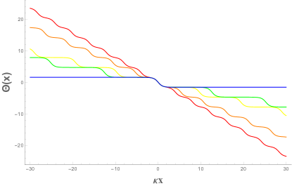
Figure 13: These are plots of the profile $\Theta(x)$ for the lowest energy spiral solution, $A$ given by Eq. (106), at several values of $k$: Red $k=\frac{98}{100}$, Orange $k=\frac{998}{100}$, Yellow $k=\frac{999998}{1000000}$, Green $k=\frac{99999998}{100000000}$, and Blue $k=1$. As the modulus $k$ increases $\Theta(x)$ tends towards a domain wall configuration, achieving it for $k=1$.

As can be seen in Fig. 13, the domain wall solution connects $\Theta=\frac{\pi}{2}$ at $x=-\infty$ to $\Theta=-\frac{\pi}{2}$ at $x=\infty$. Since one period of the spiral solution should span $\Delta\Theta=-2\pi$, the infinite period limit of the one period of spiral solution contains two domain wall solutions. These are the long and short domain wall configurations of Equations. (73) and (75).

One period of the spiral solution (101) reduces to the following domain wall solution in the limit of infinite period $k\to 1$ corresponding to $A=\frac{(\pi\kappa)^{2}}{8}$

$$\begin{split}\Theta&=-2\arctan\left(\exp(\sqrt{2A}x)\right)+\frac{\pi}{2},\\ \vec{n}^{\alpha}&=\left(0,-\tanh\left(\sqrt{2A}x\right),\operatorname{sech}\left(\sqrt{2A}x\right)\right)^{T}.\end{split}$$ (108)

We note that this is a domain wall solution for any $A>0$ with $B=0$. The total energy of the domain wall is zero at $A=\frac{(\pi\kappa)^{2}}{8}$, positive for $A>\frac{(\pi\kappa)^{2}}{8}$, and negative in the spiral phase $A<\frac{(\pi\kappa)^{2}}{8}$.

B.1.2 Case of negative anisotropy ($A<0$)

This is formally the same as the previous case. However, the elliptic modulus is changed which modifies some of the results. In the case of $A<0,B=0$, we define $\hat{\Theta}=\Theta+\frac{\pi}{2}$ to obtain

$$\sqrt{2C_{0}}(x-x_{0})=-\int_{{\hat{\Theta}}(x_{0})}^{{\hat{\Theta}}(x)}\frac{d{\hat{\Theta}}}{\sqrt{1-k^{2}\sin^{2}{\hat{\Theta}}}}\;,$$ (109)

where the modulus of the elliptic integral $k$ is given by

$$k=\sqrt{\frac{-A}{C_{0}}},$$ (110)

and the solution is given by means of Jacobi elliptic function as

$$\cos\Theta=\sin{\hat{\Theta}}=-{\rm sn}\left(\sqrt{2C_{0}}x,k\right),$$ (111)

where the NG mode is chosen as $\Theta(x_{0}=0)=\frac{\pi}{2}$. To find the expressions in this case simply take the expressions for the Period and energy density in the $A>0$ case and replace $C_{0}+A$ by $C_{0}$. Doing this we find that the lowest energy spiral solution occurs when $f(C_{0};A<0,B=0)=0$, giving

$$A=-\frac{\pi^{2}\kappa^{2}}{8}\left(\frac{k}{E(k)}\right)^{2}.$$ (112)

Combining with Eq. (61), we find $C_{0}(A)$ as a function of $A$, which determines $C_{0}(A)$ as a function of $A$. The minimum energy is given by

$$\langle\mathcal{E}\rangle=-C_{0}(A).$$ (113)

As $C_{0}$ approaches the lowest allowed value $-U_{\rm min}=A<0$, the period $L$ becomes infinite, $f(C_{0}=0;A<0,B=0)=0$, and the lowest energy spiral solution has the same average energy density as the homogeneous solution. This phase boundary of spiral and homogeneous phases occurs at the $C_{0}\to A$ limit of the minimum energy condition (112) as

$$A=-\frac{\pi^{2}}{8}\kappa^{2}.$$ (114)

The domain wall solution in this case connects $\Theta=\pi$ at $x=-\infty$ to $\Theta=0$ at $x=\infty$. Since one period of the spiral solution should span $\Delta\Theta=-2\pi$, the infinite period limit of one period of the spiral solution contains two domain wall solutions. These are a long domain wall plus a short domain wall.

B.2 Spiral solutions without anisotropy ($A=0$)

Eq. (65) is solved using $\tilde{\Theta}=\frac{\Theta+\pi}{2}$

$$\sqrt{\frac{C_{0}+B}{2}}(x-x_{0})=-\int_{\tilde{\Theta}(x_{0})}^{\tilde{\Theta}(x)}\frac{d\tilde{\Theta}}{\sqrt{1-k^{2}\sin^{2}\tilde{\Theta}}}\;,$$ (115)

where the modulus of the elliptic integral $k$ is given by

$$k=\sqrt{\frac{2B}{C_{0}+B}}.$$ (116)

We find that $k<1$ for $C_{0}>-U_{\rm min}=B$. The monotonically decreasing solutions can be expressed in terms of a Jacobi elliptic function gradshtein2007 as

$$\cos\frac{\Theta}{2}=-{\rm sn}\left(\sqrt{\frac{C_{0}+B}{2}}x,k\right),$$ (117)

where the NG mode is chosen such that $\Theta(x_{0}=0)=-\pi$. The period $L$, the excess energy $f(C_{0};A=0,B)$ in a period, and the average energy density $\langle\mathcal{E}\rangle$ of the spiral solution are given as

$$L=2\sqrt{\frac{2}{C_{0}+B}}K(k),$$ (118)

$$f(C_{0};A=0,B)=-2\pi\kappa+4\sqrt{2(C_{0}+B)}E(k),$$ (119)

$$\langle\mathcal{E}\rangle=\frac{f(C_{0},A=0,B)}{L}-C_{0},$$ (120)

respectively. The lowest energy spiral solution occurs when $f(C_{0};A=0,B)=0$, giving

$$B=\frac{\pi^{2}\kappa^{2}}{16}\left(\frac{k}{E(k)}\right)^{2},$$ (121)

which determines $C_{0}(B)$ as a function of $B$. The minimum energy is given by

$$\langle\mathcal{E}\rangle=-C_{0}(B),$$ (122)

which is lower than the positively polarized ferromagnetic state with the energy density $-B$.

As $C_{0}$ approaches the lowest allowed value $-U_{\rm min}=B$, the period $L$ becomes infinite, $f(C_{0}=-B;A=0,B)=0$, and the lowest energy spiral solution has the same average energy density as the ferromagnetic state. This phase boundary of spiral and ferromagnetic phases occurs at the $C_{0}\to-B$ limit of the minimum energy condition (121). Taking into account the different unit conventions used when writing down the effective energy density (23), our result on the critical magnetic field (121)agrees with the previous result for $A=0$ BH . In Fig. 14, the profile function $\Theta(x)$ given in Eq. (117) is plotted for several values of $k$ near the phase transition $B=\frac{\pi^{2}\kappa^{2}}{16}$.

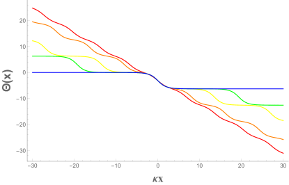
Figure 14: These are plots of the profile $\Theta(x)$ against the dimensionless quantity $\kappa x$ for the lowest energy spiral configurations with $B(k)$ given by Eq. (121) , for several values of $k$: Red $k=\frac{9}{10}$, Orange $k=\frac{98}{100}$, Yellow $k=\frac{9998}{10000}$, Green $k=\frac{999998}{1000000}$, and Blue $k=1$. As the parameter $k$ increases $\Theta(x)$ tends towards a sine-Gordon domain wall configuration, achieving it for $k=1$.

As can be seen in Fig. 14, the domain wall solution connects $\Theta=0$ at $x=-\infty$ to $\Theta=-2\pi$ at $x=\infty$. The infinite period limit of one period of a spiral solution contains a single domain wall in this case.

References

- (1) N. Nagaosa and Y. Tokura, “Topological Properties and Dynamics of Magnetic Skyrmions,” Nature Nanotechnology 8 (2013 ) 899–911, doi:10.1038/NNANO.2013.243.
- (2) X. Z. Yu, Y. Onose, N. Kanazawa, J. H. Park, J. H. M. Han and Y. Matsui, N. Nagaosa, Y. Tokura, “Real-space observation of a two-dimensional skyrmion crystal,” Nature 465 (2010) 901–904,
- (3) S. Muhlbauer B. Binz, F. Jonietz, C. Pfleiderer, A. Rosch, A. Neubauer, R. Georgii and P. Boni, “Skyrmion Lattice in a Chiral Magnet,” Science 323 (2009) 915–919, doi:10.1126/science.1166767
- (4) N. Romming, C. Hanneken, M. Menzel, J. E. Bickel, B. Wolter, K. von Bergmann, A. Kubetzka, and R. Wiesendanger, “Writing and Deleting Single Magnetic Skyrmions,” Science 341 (2013) 636–639, doi:10.1126/science.1240573,
- (5) I. Dzyaloshinskii, “A Thermodynamic Theory of ‘Weak’ Ferromagnetism of Antiferromagnetics,” J. Phys. Chem. Solids 4 (1958) 241–255, doi:10.1016/0022-3697(58)90076-3.
- (6) T. Moriya, “Anisotropic Superexchange Interaction and Weak Ferromagnetism,” Phys. Rev. 120 (1960) 91–98, doi:10.1103/PhysRev.120.91.
- (7) J. Kishine and A.S. Ovchinnikov, “Chapter One - Theory of Monoaxial Chiral Helimagnet,” Solid State Physics 66 (2015) 1–130, doi:https://doi.org/10.1016/bs.ssp.2015.05.001,
- (8) A. A. Tereshchenko, A. S. Ovchinnikov, I. Proskurin, E. V. Sinitsyn and J. Kishine, “Theory of magnetoelastic resonance in a monoaxial chiral helimagnet,” Physical Review B97, (2018) 184303, doi:10.1103/PhysRevB.97.184303,
- (9) S. Lin, A. Saxena and C. D. Batista “Skyrmion fractionalization and merons in chiral magnets with easy-plane anisotropy,” Phys. Rev. B, 91, 224407 (2015)
- (10) J. Müller, A. Rosch and M. Garst, “Edge instabilities and skyrmion creation in magnetic layers,” New Journal of Physics, 18 (2016).
- (11) T. Brauner and N. Yamamoto, “Chiral Soliton Lattice and Charged Pion Condensation in Strong Magnetic Fields,” JHEP 04 (2017), 132 doi:10.1007/JHEP04(2017)132, [arXiv:1609.05213 [hep-ph]].
- (12) K. Nishimura and N. Yamamoto, “Topological term, QCD anomaly, and the chiral soliton lattice in rotating baryonic matter,” JHEP 07 (2020) no.07, 196 doi:10.1007/JHEP07(2020)196, [arXiv:2003.13945 [hep-ph]].
- (13) P. G. de Gennes and J. Prost, The Physics of Liquid Crystals. Oxford: Clarendon Press, (1993).
- (14) I. Dierking, Textures of Liquid Crystals. Weinheim: Wiley-VCH,(2003).
- (15) P. J. Collings and M. Hird, Introduction to Liquid Crystals. Bristol, PA: Taylor & Francis, (1997).
- (16) D. Foster, C. Kind, P. J. Ackerman, J. S. B. Tai, M. R. Dennis, and I. I. Smalyukh, Two-dimensional skyrmion bags in liquid crystals and ferromagnets, Nature Phys. 15, 655 (2019).
- (17) A. Bogdanov and D. A. Yablonskii, “Thermodynamically stable vortices in magnetically ordered crystals. the mixed state of magnets,” Zh. Eksp. Teor. Fiz 95, 178 (1989).
- (18) A. Bogdanov and A. Hubert, “Thermodynamically stable magnetic vortex states in magnetic crystals,” Journal of Magnetism and Magnetic Materials, 138, 255-269 (1994).
- (19) J. H. Han, J. Zang, Z. Yang, J-H. Park, and N. Nagaosa, “Skyrmion lattice in a two-dimensional chiral magnet,” Physical Review B82, (2010) 094429, doi:10.1103/physrevb.82.094429,
- (20) A. N. Bogdanov, U. K. Rößler, M. Wolf, and K. H. Müller, “Magnetic structures and reorientation transitions in noncentrosymmetric uniaxial antiferromagnets,” Physical Review B, 66, 21 (2002).
- (21) A. N. Bogdanov and A. A. Shestakov “Magnetic-field-induced phase transitions between helical structures in noncentrosymmetric uniaxial antiferromagnets.” Low Temperature Physics 25, 76 (1999).
- (22) M. Hongo, T. Fujimori, T. Misumi, M. Nitta and N. Sakai, “Instantons in Chiral Magnets,” Phys. Rev. B 101, no.10, 104417 (2020) doi:10.1103/PhysRevB.101.104417, [arXiv:1907.02062 [cond-mat.mes-hall]].
- (23) M. Hongo, T. Fujimori, T. Misumi, M. Nitta and N. Sakai, “Effective field theory of magnon: Dynamics in chiral magnets and Schwinger mechanism,” [arXiv:2009.06694 [cond-mat.mes-hall]].
- (24) James Rowland, Sumilan Banerjee, and Mohit Randeria, Skyrmions in chiral magnets with Rashba and Dresselhaus spin-orbit coupling, Phys. Rev. B93, 020404 (2016).
- (25) C. A. Condat, R. A. Guyer and M. D. Miller. “Double sine-Gordon chain,” Phys Rev B. 27(1983): 474-494
- (26) M. Eto, M. Kurachi and M. Nitta, “Constraints on two Higgs doublet models from domain walls,” Phys. Lett. B 785, 447-453 (2018) doi:10.1016/j.physletb.2018.09.002, [arXiv:1803.04662 [hep-ph]].
- (27) M. Eto, M. Kurachi and M. Nitta, “Non-Abelian strings and domain walls in two Higgs doublet models,” JHEP 08, 195 (2018) doi:10.1007/JHEP08(2018)195, [arXiv:1805.07015 [hep-ph]].
- (28) C. Chatterjee, M. Haberichter and M. Nitta, “Collective excitations of a quantized vortex in superfluids in neutron stars,” Phys. Rev. C 96, no.5, 055807 (2017) doi:10.1103/PhysRevC.96.055807, [arXiv:1612.05588 [nucl-th]].
- (29) B. Barton-Singer, C. Ross and B. J. Schroers, “Magnetic Skyrmions at Critical Coupling,” Magnetic Skyrmions at Critical Coupling. Commun. Math. Phys. 375, 2259-2280 (2020). doi:10.1007/s00220-019-03676-1, arXiv:1812.07268 [cond-mat.str-el].
- (30) B. Schroers, “Solvable Models for Magnetic Skyrmions,” arXiv:1910.13907 [cond-mat.mes-hall].
- (31) C. Ross, N. Sakai and M. Nitta, “Skyrmion interactions and lattices in chiral magnets: analytical results,” JHEP. 95 (2021). doi:10.1007/JHEP02(2021)095 ,arXiv:2003.07147 [cond-mat.mes-hall].
- (32) J. Chovan, N. Papanicolaou, and S. Komineas, “Intermediate phase in the spiral antiferromagnet ,” Phys. Rev. B 65, 064433 (2002).
- (33) L. Döring and C. Melcher, Compactness Results for “Static and Dynamic Chiral Skyrmions near the Conformal Limit,” Calc. Var. (2017) 56:60, doi:10.1007/s00526-017-1172-2.
- (34) C. Melcher. “Chiral skyrmions in the Plane,” Proc. R. Soc. A 470: 20140394.
- (35) Gradshteyn, I. S. and Ryzhik, I. M.. Table of integrals, series, and products. Seventh : Elsevier/Academic Press, Amsterdam, 2007.
- (36) M. Kobayashi and M. Nitta, “Interpolating relativistic and nonrelativistic Nambu-Goldstone and Higgs modes,” Phys. Rev. D 92, no.4, 045028 (2015) doi:10.1103/PhysRevD.92.045028, [arXiv:1505.03299 [hep-th]].
- (37) M. Kobayashi and M. Nitta, “Nonrelativistic Nambu-Goldstone Modes Associated with Spontaneously Broken Space-Time and Internal Symmetries,” Phys. Rev. Lett. 113, no.12, 120403 (2014) doi:10.1103/PhysRevLett.113.120403, [arXiv:1402.6826 [hep-th]].
- (38) G. Paterson, A. Tereshchenko, S. Nakayama, Y. Kousaka, J. Kishine, S. McVitie, A. S. Ovchinnikov, I. Proskurin and Y. Togawa. “Tensile deformations of the magnetic chiral soliton lattice probed by Lorentz transmission electron microscopy,” Physical Review B 101 (2020): 184424.
- (39) Yu. A. Izyumov, V.M. Laptev, “Neutron diffraction by incommensurate magnetic structures,” Zb. Eksp. Teor. Fi. 85, 2185 (1983) [JETP 58, 1267 (1983)].