Clinical Temporal Relation Extraction with Probabilistic Soft Logic Regularization and Global Inference

Abstract

There has been a steady need in the medical community to precisely extract the temporal relations between clinical events. In particular, temporal information can facilitate a variety of downstream applications such as case report retrieval and medical question answering. However, existing methods either require expensive feature engineering or are incapable of modeling the global relational dependencies among the events. In this paper, we propose Clinical Temporal ReLation Exaction with Probabilistic Soft Logic Regularization and Global Inference (CTRL-PG), a novel method to tackle the problem at the document level. Extensive experiments on two benchmark datasets, I2B2-2012 and TB-Dense, demonstrate that CTRL-PG significantly outperforms baseline methods for temporal relation extraction.

Introduction

Clinical case reports (CCRs) are written descriptions of the unique aspects of a particular clinical case (Cabán-Martinez and García-Beltrán 2012; Caufield et al. 2018). They are intended to serve as educational aids to science and medicine, as they play an essential role in sharing clinical experiences about atypical disease phenotypes and new therapies (Caufield et al. 2018). There is a perennial need to automatically and precisely curate the clinical case reports into structured knowledge, i.e. extract important clinical named entities and relationships from the narratives (Aronson and Lang 2010; Savova et al. 2010; Soysal et al. 2018; Caufield et al. 2019; Alfattni, Peek, and Nenadic 2020). This would greatly enable both doctors and patients to retrieve related case reports for reference and provide a certain degree of technical support for resolving public health crises like the recent COVID-19 pandemic. Clinical reports describe chronicle events, elucidating a chain of clinical observations and reasoning (Sun, Rumshisky, and Uzuner 2013; Chen, Podchiyska, and Altman 2016). Extracting temporal relations between clinical events is essential for the case report retrieval over the patient chronologies. Besides, medical question answering systems require the precise ordering of clinical events in a time series within each document.

In this paper, we tackle the temporal relation extraction problem in clinical case reports.

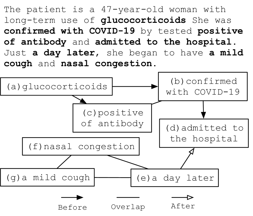
Figure 1: An illustration of a clinical case report with its partial temporal graph where transitivity dependencies exist.

Figure 1 illustrates a paragraph from a typical CCR document with three common types of temporal relations, “Before”, “After”, and “Overlap”. Glucocortocoids was described as the medicine history of this patient, which happened before confirmed with COVID-19 and positive of antibody. An “Overlap” temporal relation exists between nasal congestion and a mild cough. We consider the aforementioned clinical concepts as events, while regarding a day later as a time expression. A temporal relation may exist between event and event (E-E), event and time expression (E-T) or time expression and time expression (T-T).

There is a consensus within the clinical community regarding the difficulty of temporal information extraction, due to the high demand for domain knowledge and high complexity of clinical language representations  (Galvan et al. 2018). Meng and Rumshisky (2018); Lee et al. (2016) apply machine learning models with lexical, syntactic features, or pre-trained word representations to tackle the problem but neglect the strong dependencies between narrative containment and temporal order, thus predicting inconsistent output labels and garbled time-lines (Leeuwenberg and Moens 2017).

The dependency is the key enabler of classifying the temporal relations. For instance in Figure 1, given that b happened before d, e happened after d and e happened simultaneously with f , we can infer according to the temporal transitivity rule that b was before f. Some recent studies (Leeuwenberg and Moens 2017; Ning, Feng, and Roth 2017; Han, Zhou, and Peng 2020) convert the task to a structured prediction problem and solve it with Maximum a posteriori Inference. Integer Linear Programming (ILP) with hard constraints is deployed for optimization, which however needs an off-the-shelf solver to tackle the NP-hard optimization problem and can only approximate the optimum via relaxation. Besides, globally inferring the relations at the document level would also be intractable for them due to the high complexity and low scalability (Bach et al. 2017).

Recently, some researchers (Deng and Wiebe 2015; Chen et al. 2019; Hu et al. 2016) have explored Probabilistic Soft Logic (PSL) (Bach et al. 2017) to tackle the structured prediction problem. Inspired by them, we propose to leverage the PSL rules to model relation extraction more flexibly and efficiently. In specific, we summarize common transitivity and symmetry patterns of temporal relations as PSL rules and penalize the training instances that violate any of those rules. Different from ILP solutions, no off-the-shelf solver is required and the algorithm conducts the training process with linear time complexity. Besides, logical propositions in PSL can be interpreted not just as $true$ or $false$, but as continuously valued in the $[0,1]$ interval. We also propose a simple but effective time-anchored global temporal inference algorithm to classify the relations at the document level. With such a mechanism, we can easily verify some relations, such as the relation between b and f, with long-term dependencies which are intractable with existing approaches. As a summary, our main contributions are list as follows:

• To the best of our knowledge, this is the first work to formulate the probabilistic soft logic rules of temporal dependencies as a regularization term to jointly learn a relation classification model,

• We show the efficacy of globally inferring the temporal relations with the time graphs,

• We release the codes to facilitate further developments by the research community.

Next, we give the problem definition and explain how we leverage PSL rules to model the temporal dependencies. We then describe the overall architecture of our clinical temporal relation extraction model, CTRL-PG and show the extensive experimental results in the following sections.

Preliminaries

Problem Statement

Document $D$ contains sequences $[s_{1},s_{2},...,s_{M}]$ and named entities $x_{i}\in\mathcal{E}\bigcup\mathcal{T},1\leq i\leq N$, where $M,N$ are the total number of sequences and entities in $D$. $\mathcal{E}$ and $\mathcal{T}$ represent the set of events and time expressions, respectively. There is a potential temporal relation between any pair of annotated named entities $(x_{j},x_{k})$, where $1\leq j,k\leq N$. Formally, the task is modeled as a classification problem with a set of temporal relation types $\mathcal{Y}$. Given a sequence $s_{i}$ together with two named entities $x_{i,1},x_{i,2}$ included, we predict the temporal relation $y_{i}\in\mathcal{Y}$ from $x_{i,1}$ to $x_{i,2}$. In practice, we create a triplet with three pairs of entities to be one training instance $\mathcal{I}$, to enable the PSL rule grounding, as explained in the following section.

Probabilistic Soft Logic and Temporal Dependencies in Clinical Narratives

Here, we introduce some concepts and notations for the language PSL and illustrate how PSL is applicable to define templates for temporal dependencies and to help jointly learn a relation classifier.

Definition 1.

A predicate $\tilde{p}$ is a relation defined by a unique identifier and an atom $\tilde{l}$ is a predicate combined with a sequence of terms of length equal to the predicate’s argument number. Atoms in PSL take on continuous values in the unit interval $[0,1]$.

Example 1.

$\underline{\text{Before}}/2$ indicates a predicate taking two arguments, and the atom $\underline{\text{Before}}(A,B)$ represents whether $A$ happens before $B$.

Definition 2.

A PSL rule $\tilde{r}$ is a disjunctive clause of atoms or negative atoms:

$$\eta_{r}:T_{1}\land T_{2}\land...\land T_{m}\rightarrow H_{1}\lor H_{2}\lor...\lor H_{n},$$ (1)

where $T_{1},T_{2},...,T_{m},H_{1},H_{2},...,H_{n}$ are atoms or negative atoms.

We name $T_{1},T_{2},...,T_{m}$ as $r_{body}$ and $H_{1},H_{2},...,H_{n}$ as $r_{head}$. $\eta_{r}\in[0,1]$ is the weight of the rule $r$, denoting the prior confidence of this rule. To the opposite, an unweighted PSL rule is to describe a constraint that is always true. The unweighted logical clauses in Table 1 describe the common temporal transitivity and symmetry dependencies we summarize from the clinical narratives.

Abbrev.	PSL rules
Transitivity Dependencies
BBB	Before$(A,B)$ $\land$ Before$(B,C)$ $\rightarrow$ Before$(A,C)$
BOB	Before$(A,B)$ $\land$ Overlap$(B,C)$ $\rightarrow$ Before$(A,C)$
OBB	Overlap$(A,B)$ $\land$ Before$(B,C)$ $\rightarrow$ Before$(A,C)$
OOO	Overlap$(A,B)$ $\land$ Overlap$(B,C)$ $\rightarrow$ Overlap$(A,C)$
AAA	After$(A,B)$ $\land$ After$(B,C)$ $\rightarrow$ After$(A,C)$
AOA	After$(A,B)$ $\land$ Overlap$(B,C)$ $\rightarrow$ After$(A,C)$
OAA	Overlap$(A,B)$ $\land$ After$(B,C)$ $\rightarrow$ After$(A,C)$
Symmetry Dependencies
BA	Before$(A,B)$ $\rightarrow$ After$(B,A)$
AB	After$(A,B)$ $\rightarrow$ Before$(B,A)$
OO	Overlap$(A,B)$ $\rightarrow$ Overlap$(B,A)$

Table 1: Temporal transitivity and symmetry PSL rules $\mathcal{R}$. $A,B,C$ are three terms representing either events or time expressions.

Definition 3.

The ground atom $l$ and ground rule $r$ are particular variable instantiation of some atom $\tilde{l}$ and rule $\tilde{r}$, respectively.

Example 2.

That Overlap (e, f) $\land$ Overlap (f, g) $\rightarrow$ Overlap (e, g) from Figure 1 is a ground rule composed of three ground atoms, denoted as $l_{1},l_{2}$, and $l_{3}$, respectively. It is grounded from the OOO rule, as shown in Table 1.

Definition 4.

The interpretation $I(l)$ denotes the soft truth value of an atom $l$.

Definition 5.

Łukasiewicz t-norm (Klir and Yuan 1995) is used to define the basic logical operations in PSL, including logical conjunction ($\land$), disjunction ($\lor$), and negation ($\neg$):

$$I(l_{1}\land l_{2})=\max\{I(l_{1})+I(l_{2})-1,0\}$$ (2)

$$I(l_{1}\lor l_{2})=\min\{I(l_{1})+I(l_{2}),1\}$$ (3)

$$I(\neg l_{1})=1-I(l_{1})$$ (4)

The PSL rule in Definition 2 can also be represented as:

$$I(r_{body}\rightarrow r_{head})=I(\neg r_{body}\lor r_{head}),$$

so we can induce the distance to satisfaction for rule $r$.

Definition 6.

The distance to satisfaction $d_{r}(I)$ of rule $r$ under an interpretation $I$ is defined as:

$$d_{r}(I)=\max\{0,I(r_{body})-I(r_{head})\}$$ (5)

PSL program determines a rule $r$ as satisfied when the truth value of $I(r_{head})-I(r_{body})\geq 0$.

Example 3.

Given that $I(l_{1})=0.7,I(l_{2})=0.8,$ and $I(l_{3})=0.3$, we can compute the distance according to Equation (2)-(5):

$$d_{r}=\max\{0,I(l_{1}\land l_{2})-I(l_{3})\}$$

$$=\max\{0,0.7+0.8-1-I(l_{3})\}$$

$$=\max\{0,0.5-0.3\}$$

$$=0.2$$

This equation indicates that the ground rule in Example 2 is completely satisfied when $I(l_{3})$ is above $0.5$. Otherwise, a penalty factor will be raised ($0.2$ in this case). When $I(l_{3})$ is under $0.5$, the smaller $I(l_{3})$ is, the larger penalty we have. In short, we compute the distance to satisfaction for each ground rule as a loss regularization term to jointly learn a relation classification model. We finally use the smallest one as the penalty because we only need one of the rules to be satisfied.

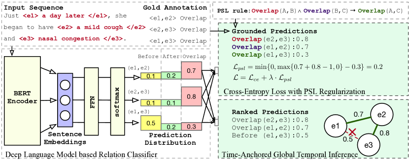
Figure 2: The overall architecture of CTRL-PG. We leverage the cross-entropy function and PSL regularization to jointly train a relation classifier with the sentence embeddings from a deep language model and perform global temporal inference with a time graph. We acquire the prediction probability distributions from a deep language model based relation classifier to compute the distance loss $\mathcal{L}_{psl}$ in the PSL module and time graph construction in the global inference module.

Clinical Temporal Relation Extraction

Figure 2 shows the overall framework of the proposed CTRL-PG model. The framework consists of three components, (i) a temporal relation classifier composed of a deep language encoder and a Feed-Forward Network (FFN), (ii) a Cross-Entropy loss function with PSL regularization, and (iii) a time-anchored global temporal inference module. We will introduce the details of the three modules in the following subsections.

Temporal Relation Classifier

The context is essential for capturing the syntactic and semantic features of each word in a sequence. Hence, we propose to apply the contextualized language model, BERT (Devlin et al. 2018), to derive the sentence representation $v_{i}$ of $d_{s}$-dimension to encode the input sequence $s_{i}$ including two marked named entities $x_{i,1},x_{i,2}$ from the instance $\mathcal{I}$, where $i\in\{1,2,3\}$. We group three sequences together to facilitate the computation of regularization term introduced in the next subsection.

By feeding the sentence embedding $v_{i}$ to a layer of FFN, we can predict the relation type $\hat{y_{i}}$ with the softmax function:

$$\hat{y}_{i}=\operatorname*{argmax}_{y\in\mathcal{Y}}\;\mathbb{P}(y|s_{i})$$ (6)

$$\mathbb{P}(y|s_{i})=\text{softmax}(W_{f}\cdot v_{i}+b_{f}),$$ (7)

where $W_{f}$ and $b_{f}$ are the weights and bias in the FFN layer.

To learn the relation classification model, we first compute a loss with the Cross-Entropy objective for each instance $\mathcal{I}$:

$$\mathcal{L}_{ce}=-\sum_{i\in\{1,2,3\}}\sum_{y\in\mathcal{Y}}y\log\mathbb{P}(y|s_{i})$$ (8)

Learning with Probabilistic Soft Logic Regularization

We also aim to minimize the distance to rule satisfaction for each instance. We compute the distance with function $\mathcal{F}(\cdot,\cdot)$, as described in Algorithm 1, by finding the minimum of all possible PSL rule grounding results, i.e., when one PSL rule is satisfied, $\mathcal{F(\cdot,\cdot)}$ should return $0$. In specific, we first ground the three relation predictions $\hat{y}_{i}$ with potential PSL rules. We then incorporate Equation (2)-(5) for distance computation. The prediction probabilities are regarded as the interpretation of the ground atoms $l_{i}$. If none of the rules can be grounded, the distance will be set as 0.

Input: PSL Rules $\mathcal{R}$, Prediction $\hat{y}_{i}$, and Probability $\mathbb{P}(y|s_{i})$, $i=\{1,2,3\}$;

Output: Distance $d_{r}$;

Set $d_{r}=1$; $d_{t}=0$; IsGround $=false$;

for each $l_{1}\land l_{2}\to l_{3}\in\mathcal{R}$ do

       if $\hat{y}_{1}$ matches $l_{1}$ and $\hat{y}_{2}$ matches $l_{2}$ then

             Determine $\bar{y}_{3}$ with $l_{3}$;

             $d_{t}\leftarrow\max\{\mathbb{P}(y=\hat{y}_{1}|s_{1})+\mathbb{P}(y=\hat{y}_{2}|s_{2})-1,0\}$;

             $d_{t}\leftarrow\max\{d_{t}-\mathbb{P}(y=\bar{y}_{3}|s_{3}),0\}$;

             $d_{r}\leftarrow\min\{d_{r},d_{t}\}$;

             IsGround $\leftarrow true$;

            

      

end for

if IsGround $==false$ then

      $d_{r}\leftarrow 0$;

Algorithm 1 Function $\mathcal{F}$ for PSL Rule Grounding and Distance Calculation.

Then, we formulate the distance to satisfaction as a regularization term to penalize the predictions that violate any PSL rule:

$$\mathcal{L}_{psl}=\mathcal{F}(\mathcal{R};\{(\mathbb{P}(y|s_{i}),\hat{y}_{i})\}),i=\{1,2,3\}$$ (9)

and finalize the loss function by summing up (8) and (9):

$$\mathcal{L}=\mathcal{L}_{ce}+\lambda\cdot\mathcal{L}_{psl},$$ (10)

where $\lambda$ is a hyperparameter as the weight for PSL regularization term. We apply gradient descent to minimize the loss function (10) and to update the parameters of our model.

Global Temporal Inference

In the inference stage, we leverage the Timegraph algorithm (Miller and Schubert 1990) to resolve the conflicts in the temporal relation predictions $\bm{\hat{y}}$. Timegraph is a widely used algorithm of time complexity $\mathcal{O}(v+e)$ for deriving the temporal relation for any two nodes in a connected graph, where $v$ and $e$ denote the numbers of nodes and edges. Nodes and edges represent the named entities and temporal relations, respectively. Our goal is to construct a conflict-free time graph $\mathcal{G}$ for each document $D$ through a greedy Check-And-Add process, described as $4$ steps in Algorithm 2. Intuitively, we want to rely on some trustworthy edges to resolve the conflicts in the time graph with the transitivity and symmetry dependencies listed in Table 1. As illustrated in Figure 2, the probabilities of predictions Overlap(e1, e2) and Overlap(e2, e3) are $0.7$ and $0.8$, which are higher than that of Overlap(e1, e3). When we trust the first two predictions, the third prediction could be neglected considering the relation between e1 and e3 can already be inferred with the transitivity dependency. In this way, the predicting mistakes with low confidence scores can be ruled out, leading to better model performance in the closure evaluation.

We believe that the relations between time expressions are the easiest ones to predict. For example, the ground atom Before (06-15-91, July 1st 1991) is obviously $true$. Therefore, we try to build up a base time graph on top of the relations of type T-T. Next, we rank the rest of the predictions according to their probabilities in decreasing order and then check whether each of the predictions is inconsistent with the current time graph iteratively. The relation will be dropped if it raises a conflict, otherwise added to the graph as a new edge.

Step 1: Predict temporal relations $P_{1}$ on pairs of the time expressions T-T;

Step 2: Construct a time graph $\mathcal{G}$ with $P_{1}$;

Step 3: Rank all other predictions $P_{2}$ on the relations of type E-E and E-T according to the predicting probabilities in decreasing order, naming $P_{2}^{ranked}$;

Step 4:

for each $p$ in $P_{2}^{ranked}$ do

       Apply Timegraph algorithm to check the conflict between $p$ and $\mathcal{G}$;

       if there exists a conflict then

            Drop $p$;

       else

            Add the edge $p$ to $\mathcal{G}$;

       end if

      

end for

Algorithm 2 Check-And-Add Process for Constructing a Conflict-free Time Graph $\mathcal{G}$

Experiments

In this section, we develop experiments on two benchmark datasets to prove the effectiveness of both PSL regularization and global temporal inference. We also discuss the limitation and perform error analyses for CTRL-PG.

Dataset		Train	Dev	Test
I2B2-2012	# doc	181	9	120
	# relation	29,736	1,165	24,971
TB-Dense	# doc	22	5	9
	# relation	4,032	629	1,427

Table 2: Dataset Statistics.

Datasets

Experiments are conducted on I2B2-2012 and TB-Dense datasets and an overview of the data statistics is shown in Table 2. The datasets have diverse annotation densities and instance numbers.

I2B2-2012. The I2B2-2012 challenge corpus (Sun, Rumshisky, and Uzuner 2013) consists of 310 discharge summaries. Two categories of temporal relations, E-T and E-E, were annotated in each document. Three temporal relations, Before, After, and Overlap, were used. I2B2-2012 has a relatively low annotation density, which is $0.21$.

TB-Dense. To prove that our PSL regularization is a generic algorithm and can be easily adapted to other domains, we also test it on the TB-dense (Cassidy et al. 2014) dataset, which is based on TimeBank News Corpus (Pustejovsky et al. 2003). Annotators were required to label all pairs of events/times in a given window to address the sparse annotation issue in the original data. Thus the annotation density is 1. This dataset has six relation types, Simultaneous, Before, After, Includes, Is_Include, and Vague.

Baseline Models

We employ different baseline models for the two datasets to compare our method with the SOTA models in both clinical and news domains.

I2B2-2012 (1) Feature-engineering based statistic models from I2B2-2012 challenge, MaxEnt-SVM (Xu et al. 2013) incorporating Maximum Entropy with Support Vector Machine (SVM), CRF-SVM (Tang et al. 2013) using Conditional Random Fields and SVM, RULE-SVM (Nikfarjam, Emadzadeh, and Gonzalez 2013) relying on rule-based algorithms; (2) Neural network based model, RNN-ATT (Liu et al. 2019a), which applies Recurrent Neural Network plus attention mechanism; (3) Structured Prediction method, SP-ILP (Han et al. 2019; Leeuwenberg and Moens 2017) leveraging the ILP optimization; (4) Basic version of our model, CTRL, which only fine-tunes a BERT-BASE (Devlin et al. 2018) language model with one layer of FFN, similar to the implementations in Lin et al. (2019); Guan et al. (2020).

TB-Dense. (1) CAEVO (Chambers et al. 2014) with a cascade of rule-based classifiers; (2) LSTM-DP (Cheng and Miyao 2017) using LSTM-based network and cross-sentence dependency paths; (3) GCL (Meng and Rumshisky 2018) incorporating LSTM-based network with discourse-level contexts; (4) SP-ILP and CTRL, same as the baselines for I2B2-2012. Note that the results of CAEVO, LSTM-DP, GCL, and SP-ILP are collected from Han et al. (2019).

Evaluation Metrics

To be consistent with previous work for a fair comparison, we adopt two different evaluation metrics. For TB-Dense dataset, we compute the Precision, Recall, and Micro-average F1 scores. Following (Han, Ning, and Peng 2019; Meng and Rumshisky 2018), we only predict the E-E relations and exclude all other relations from evaluation. Note that Micro-averaging in a multi-class setting will lead to the same value for Precision, Recall, and F1. For I2B2-2012, we leverage the TempEval evaluation metrics used by the official challenge (Sun, Rumshisky, and Uzuner 2013), which also calculates the Precision, Recall, and Micro-average F1 scores. This evaluation metrics differ from the standard F1 used for TB-Dense in a way that it computes the Precision by verifying each prediction in the closure of the ground truths and computes the Recall by verifying each ground truth in the closure of the predictions. We explore all types of temporal relations in I2B2-2012 dataset.

Implementation Details

In the framework of CTRL-PG, any contextualized word embedding method, such as BERT (Devlin et al. 2018), ELMo (Peters et al. 2018), and RoBERTa (Liu et al. 2019b), can be utilized. We choose BERT (Devlin et al. 2018) to derive contextualized sentence embeddings without loss of generality. BERT adds a special token [CLS] at the beginning of each tokenized sequence and learns an embedding vector for it. We follow the experimental settings in (Devlin et al. 2018) to use $12$ Transformer layers and attention heads and set the embedding size $d_{s}$ as 768. The CTRL-PG is implemented in PyTorch and we use the fused Adam optimizer (Kingma and Ba 2014) to optimize the parameters. We follow the experimental settings in (Devlin et al. 2018) to set the dropout rate, and batch size as $10^{-1}$ and 8. We perform grid search for the initial learning rate from a range of $\{1\times 10^{-5},2\times 10^{-5},4\times 10^{-5},8\times 10^{-5}\}$ and finally select $2\times 10^{-5}$ for both datasets. We train 10 epochs for each experiment on two datasets, which can all be completed within 2 hours on single DGX1 Nvidia GPU.

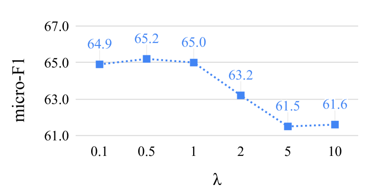
Figure 3: Hyperparameter Search for $\lambda$ on TB-Dense dataset.

To tune the hyperparameters, we search the PSL regularization term $\lambda$ from $\{0.1,0.5,1,2,5,10\}$ as shown in Figure 3. For I2B2-2012 and TB-Dense datasets, we set $\lambda$ as $5$ and $0.5$, respectively. The hyperparameters are selected by observing the best F1 performance on the validation set. More implementation details can be found in the Appendix.

Model	P	R	F1
RULE-SVM	71.09	58.39	64.12
MaxEnt-SVM	74.99	64.31	69.24
CRF-SVM	72.27	66.81	69.43
RNN-ATT	71.96	69.15	70.53
SP-ILP	78.15	78.29	78.22
CTRL	84.88	73.28	78.65
CTRL-PG	86.80	74.53	80.20

Table 3: Performance of temporal relation extraction on I2B2-2012 datasets. All improvements of CTRL-PG over baseline methods are statistically significant at a 99% confidence level in paired t-tests. Results show that CTRL-PG outperforms all the baselines.

Feature	P	R	F1	Lift
Best	86.80	74.53	80.20	-
w/o PSL	85.78	73.31	79.06	1.44%
w/o GTI	85.08	73.31	78.76	1.83%

Table 4: Ablation study on I2B2-2012 dataset. GTI denotes the global temporal inference. Results show significant performance lifts from both PSL and GTI modules.

Strategy	P	R	F1	Lift
Random	85.08	73.93	79.21	-
Confidence	86.07	73.76	79.44	0.29%
Confidence +	86.80	74.53	80.20	1.25%
Time Anchor

Table 5: Comparison of different ranking methods applied in the global inference on I2B2-2012 dataset.

1	Text	Her acute bradycardic event was felt likely secondary to her new beta blocker in conjunction with
		a vagal response . It was determined to stop the beta blocker , and atropine was placed at the bedside .
	(e1, e2)	(Her…event, her…blocker)	(her…blocker, the beta blocker)	(Her…event, the beta blocker)
	True Label	After	Overlap	After
	CRTL	After	Overlap	Overlap
	CTRL-PG	After	Overlap	After
	Rule	After$(A,B)$ $\land$ Overlap$(B,C)$ $\rightarrow$ After$(A,C)$
2	Text	The patient was given an aspirin and Plavix and in addition started on a beta Elmore , Maxine ACE
		inhibitor , and these were titrated up as her blood pressure tolerated .
	(e1, e2)	(started, a beta Elmore)	(a beta Elmore, Maxine ACE)	(started, Maxine ACE)
	True Label	Before	Overlap	Before
	CRTL	After	Overlap	Before
	CTRL-PG	After	Overlap	After
	Rule	After$(A,B)$ $\land$ Overlap$(B,C)$ $\rightarrow$ After$(A,C)$
3	Text	She has had attacks treated with antibiotics in the past notably in 12/96 and 08/97 .
	(e1, e2)	(antibiotics, 12/96)	(12/96, 08/97)	(antibiotics, 08/97)
	True Label	Overlap	Before	Overlap
	CRTL	Overlap	Before	Overlap
	CTRL-PG	Overlap	Before	Before
	Rule	Overlap$(A,B)$ $\land$ Before$(B,C)$ $\rightarrow$ Before$(A,C)$

Table 6: Case study and error analysis of the model predictions on I2B2-2012 Dataset.

	SP-ILP			CTRL-PG
	P	R	F1	P	R	F1
Before	71.1	58.9	64.4	52.6	74.8	61.7
After	75.0	55.6	63.5	69.0	72.5	70.7
Includes	24.6	4.2	6.9	60.9	29.8	40.0
Is_Include	57.9	5.7	10.2	34.7	27.7	30.8
Simultaneous	-	-	-	-	-	-
Vague	58.3	81.2	67.8	72.8	64.8	68.6
Micro-average	63.2			65.2
CAEVO	49.4
LSTM-DP	52.9
GCL	57.0
CTRL	63.6

Table 7: Performance of temporal relation extraction on TB-dense datasets. All improvements of CTRL-PG over baseline methods are statistically significant at a 99% confidence level in paired t-tests. We also compare the breakdown performance for each relation class between CTRL-PG and SP-ILP.

Experimental Results

Table 3 and Table 7 contains our main results. As we observe, our CTRL-PG enhanced by PSL regularization and global inference achieve the best relation extraction performances per F1 score. Compared with the baseline models, the F1 score improvements are 2.0% and 2.5% on I2B2-2012 and TB-Dense data respectively, which are all statistically significant.

I2B2-2012. As shown in Table 3, our model CTRL-PG outperforms the best baseline method CTRL by 2% and outperforms the structured prediction method SP-ILP by 2.5% per F1 score. SP-ILP gets the highest Recall score, but sacrifice the predicting precision instead. We also observe that by simply fine-tuning the BERT to generate the sentence embeddings and then feeding them into one layer of FFN for classification, CTRL can achieve an impressive F1 score of 78.65%. This proves the advantage of contextualized embeddings over static embeddings used by other baseline models. Besides, CTRL-PG outperforms the feature-based systems, CRF-SVM and MaxEnt-SVM, by over 10% per F1 score.

We develop an ablation study to test different features, as shown in Table 4. We see that PSL regularization and global temporal inference modules lift the performance by 1.44% and 1.83% separately. Both Precision and Recall performances are improved. We can clearly conclude that learning the relations with the proposed algorithms improves our model significantly (also at a 99% level in paired t-tests).

We also show the comparisons among different ranking strategies for the global inference module in Table 5. Random denotes that we randomly add a new prediction to the time graph and resolve the conflict. Confidence denotes we rank the predictions per the prediction probabilities and then add them to the graph in decreasing order. Time Anchor represents that we first construct the time graph based on the predictions for temporal relations of type T-T. In the results, we see a 0.29% improvement per F1 score when switching from the Random to the Confidence strategy. After adding the Time Anchor method, we observe a 1.25% performance lift, compared to Random strategy. This proves the effectiveness of the time-anchored global temporal inference module.

TB-Dense. We show the experimental results on TB-Dense dataset in Table 7. Our model outperforms the best baseline model CTRL by 2.5% and outperforms the structured prediction method SP-ILP by 3.2% per Micro-average F1 score. We observe that in the performance breakdown for each relation class, CTRL-PG obtains similar scores on Before, After, and Vague as SP-ILP and gets much better performances on Is_Include and Includes. These two types only occupy 5.7% and 4.5% of all the instances. CTRL-PG and SP-ILP both fail to label any instance as Simultaneous because of its even fewer instances (1.5%) for training.

Besides, we observe CTRL-PG achieves higher Recall values in all the categories of temporal relations, which prove that incorporating the dependency rules into model training can dramatically lift the coverage of predictions.

Case Study and Error Analysis.

Table 6 shows the results of a case study with the outputs of CTRL and CTRL-PG. In the first case, the temporal relation between Her acute bradycardic event and the beta blocker is hard to predict due to the noise brought by the long context. CTRL predicts it as Overlap, while CTRL-PG corrects it to After according to the potential PSL rule that can be matched with the first two correct predictions. In some cases, however, CTRL-PG will make new mistakes. For example in case 2, if our model initially predicts the relation between started and a beta Elmore wrong, a potential PSL rule sometimes will lead to an extra mistake when predicting the relation between started and Maxine ACE. In the case 3, antibiotics treated the attacks twice in both $12/96$ and $08/97$, where the PSL rule is no longer valid since the antibiotics in fact denote two occurrences of this event. In such special cases with invalid rules, CTRL-PG may make a mistake.

Related Work

Clinical Temporal Relation Extraction

Corpora. Different from the datasets in the news domain (Pustejovsky et al. 2003; Graff 2002), the corpora in the clinical domain require rich domain knowledge for annotating the temporal relations. I2b2-2012 (Sun, Rumshisky, and Uzuner 2013) and Clinical TempEval (Bethard et al. 2015, 2016, 2017) are some great efforts of building clinical datasets with extensive annotations including labels of clinical events and temporal relations, the second of which was not tested in our paper due to lack of access to the data.

Models. Some early efforts to solve the clinical relation extraction problem leverage conventional machine learning methods (Llorens, Saquete, and Navarro 2010; Sun, Rumshisky, and Uzuner 2013; Xu et al. 2013; Tang et al. 2013; Lee et al. 2016; Chikka 2016) such as SVMs, MaxEnt and CRFs, and neural network based methods (Lin et al. 2017, 2018; Dligach et al. 2017; Tourille et al. 2017; Lin et al. 2019; Guan et al. 2020; Lin et al. 2020; Galvan-Sosa et al. 2020). They either require expensive feature engineering or fail to consider the dependencies among temporal relations within a document. (Leeuwenberg and Moens 2017; Han et al. 2019; Han, Ning, and Peng 2019; Ning, Feng, and Roth 2017) formulate the problem as a structured prediction problem to model the dependencies but can not globally predict temporal relations. Instead, our method can infer the temporal relations at document level.

Probabilistic Soft Logic

In recent years, PSL rules have been applied to various machine learning topics such as Fairness (Farnadi, Babaki, and Getoor 2019), Model Interpretability (Hu et al. 2016), Probabilistic Reasoning (Augustine, Rekatsinas, and Getoor 2019; Dellert 2020), Knowledge Graph Construction (Pujara et al. 2013; Chen et al. 2019) and Sentiment Analysis (Deng and Wiebe 2015; Gridach 2020). We are the first to model the temporal dependencies with PSL.

Conclusion

In this paper, we propose CTRL-PG that leverages the PSL rules to model the temporal dependencies as a regularization term to jointly learn a relation classification model. Extensive experiments show the efficacy of the PSL regularization and global temporal inference with time graphs.

Appendix A Appendices

Dataset

The I2B2-2012 dataset is officially split into training and test sets, containing 190 and 120 documents, separately. We randomly sampled 5% of training data as a validation set. For TB-Dense, the training/validation/test sets are given. The statistics are shown in Table 2 and we plot the detailed relation type distributions of two datasets in Figure 4. We observe that TB-Dense is a relatively unbalanced dataset, where Vague dominates the dataset. We compute the density by (# existing relations)/(# possible pairs of entities). Following (Han, Ning, and Peng 2019; Meng and Rumshisky 2018), we only predict the E-E relations and exclude all other relations from evaluation for TB-Dense dataset evaluation. Therefore, we cannot apply the global inference module to this dataset.

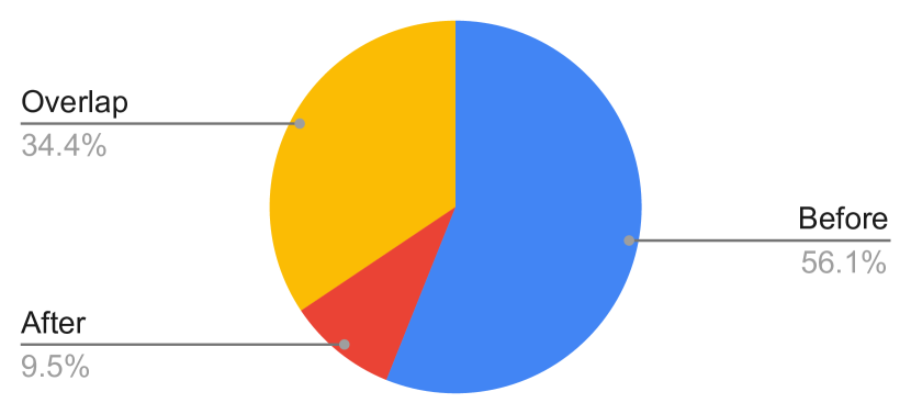
(a) I2B2-2012

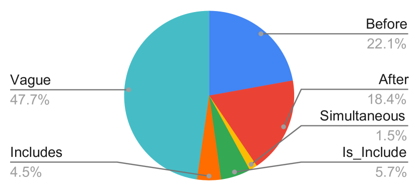
(b) TB-Dense

Figure 4: Relation Type Distribution of I2B2-2012 and TB-Dense

Data Preprocessing

To facilitate the PSL rule grounding and distance calculation, we arrange the training data as a collection of instances, each of which contains three pairs of relations. We first traverse the training dataset to match the PSL rules and make sure that each ground rule is treated as one instance to further calculate the PSL loss term. Besides, relations that are not involved in any rules are packed together and we do not have to compute a PSL loss for them. We also augment the training data by flipping every pair according to the symmetry rules, i.e. if Before($A,B$) is $true$, After($B,A$) should also be $true$. We incorporate the new relations into the training dataset to alleviate the unbalanced data issue.

Model Training Details

We leverage the pretrained BERT-BASE model (Devlin et al. 2018) to generate the sentence embeddings, which contains 110M parameters to fine-tune. In the experiments, we save the checkpoint with the highest validation performance for final testing. In Table 8, we list the best validation performance of different datasets and the corresponding test performance that we also reported in Table 3 and Table 7 for completeness. Data and codes are attached.

Dataset		Precision	Recall	F1
I2B2-2012	Test	86.80	74.53	80.20
	Val	86.03	86.03	86.03
TB-Dense	Test	65.20	65.20	65.20
	Val	58.80	58.80	58.80

Table 8: Corresponding validation performance for each reported test result of CTRL-PG in Table 3 and Table 7.

References

- Alfattni, Peek, and Nenadic (2020) Alfattni, G.; Peek, N.; and Nenadic, G. 2020. Extraction of Temporal Relations from Clinical Free Text: A Systematic Review of Current Approaches. Journal of Biomedical Informatics 103488.
- Aronson and Lang (2010) Aronson, A. R.; and Lang, F.-M. 2010. An overview of MetaMap: historical perspective and recent advances. Journal of the American Medical Informatics Association 17(3): 229–236.
- Augustine, Rekatsinas, and Getoor (2019) Augustine, E.; Rekatsinas, T.; and Getoor, L. 2019. Tractable Probabilistic Reasoning Through Effective Grounding. In Third ICML workshop on Tractable Probabilistic Modeling.
- Bach et al. (2017) Bach, S. H.; Broecheler, M.; Huang, B.; and Getoor, L. 2017. Hinge-loss markov random fields and probabilistic soft logic. The Journal of Machine Learning Research 18(1): 3846–3912.
- Bethard et al. (2015) Bethard, S.; Derczynski, L.; Savova, G.; Pustejovsky, J.; and Verhagen, M. 2015. SemEval-2015 Task 6: Clinical TempEval. In Proceedings of the 9th International Workshop on Semantic Evaluation (SemEval 2015), 806–814. Denver, Colorado: Association for Computational Linguistics. doi:10.18653/v1/S15-2136. URL https://www.aclweb.org/anthology/S15-2136.
- Bethard et al. (2016) Bethard, S.; Savova, G.; Chen, W.-T.; Derczynski, L.; Pustejovsky, J.; and Verhagen, M. 2016. SemEval-2016 Task 12: Clinical TempEval. In Proceedings of the 10th International Workshop on Semantic Evaluation (SemEval-2016), 1052–1062. San Diego, California: Association for Computational Linguistics. doi:10.18653/v1/S16-1165. URL https://www.aclweb.org/anthology/S16-1165.
- Bethard et al. (2017) Bethard, S.; Savova, G.; Palmer, M.; and Pustejovsky, J. 2017. SemEval-2017 Task 12: Clinical TempEval. In Proceedings of the 11th International Workshop on Semantic Evaluation (SemEval-2017), 565–572. Vancouver, Canada: Association for Computational Linguistics. doi:10.18653/v1/S17-2093. URL https://www.aclweb.org/anthology/S17-2093.
- Cabán-Martinez and García-Beltrán (2012) Cabán-Martinez, A. J.; and García-Beltrán, W. F. 2012. Advancing medicine one research note at a time: the educational value in clinical case reports. BMC Research Notes 5(1): 293. doi:10.1186/1756-0500-5-293.
- Cassidy et al. (2014) Cassidy, T.; McDowell, B.; Chambers, N.; and Bethard, S. 2014. An Annotation Framework for Dense Event Ordering. In Proceedings of the 52nd Annual Meeting of the Association for Computational Linguistics (Volume 2: Short Papers).
- Caufield et al. (2019) Caufield, J. H.; Zhou, Y.; Bai, Y.; Liem, D. A.; Garlid, A. O.; Chang, K.-W.; Sun, Y.; Ping, P.; and Wang, W. 2019. A Comprehensive Typing System for Information Extraction from Clinical Narratives. medRxiv 19009118.
- Caufield et al. (2018) Caufield, J. H.; Zhou, Y.; Garlid, A. O.; Setty, S. P.; Liem, D. A.; Cao, Q.; Lee, J. M.; Murali, S.; Spendlove, S.; Wang, W.; et al. 2018. A reference set of curated biomedical data and metadata from clinical case reports. Scientific data 5: 180258.
- Chambers et al. (2014) Chambers, N.; Cassidy, T.; McDowell, B.; and Bethard, S. 2014. Dense event ordering with a multi-pass architecture. Transactions of the Association for Computational Linguistics 2: 273–284.
- Chen, Podchiyska, and Altman (2016) Chen, J. H.; Podchiyska, T.; and Altman, R. B. 2016. OrderRex: clinical order decision support and outcome predictions by data-mining electronic medical records. Journal of the American Medical Informatics Association 23(2): 339–348.
- Chen et al. (2019) Chen, X.; Chen, M.; Shi, W.; Sun, Y.; and Zaniolo, C. 2019. Embedding uncertain knowledge graphs. In Proceedings of the AAAI Conference on Artificial Intelligence, volume 33, 3363–3370.
- Cheng and Miyao (2017) Cheng, F.; and Miyao, Y. 2017. Classifying Temporal Relations by Bidirectional LSTM over Dependency Paths. In Proceedings of the 55th Annual Meeting of the Association for Computational Linguistics (Volume 2: Short Papers).
- Chikka (2016) Chikka, V. R. 2016. CDE-IIITH at SemEval-2016 Task 12: Extraction of Temporal Information from Clinical documents using Machine Learning techniques. In Proceedings of the 10th International Workshop on Semantic Evaluation (SemEval-2016), 1237–1240. San Diego, California: Association for Computational Linguistics. doi:10.18653/v1/S16-1192. URL https://www.aclweb.org/anthology/S16-1192.
- Dellert (2020) Dellert, J. 2020. Exploring Probabilistic Soft Logic as a framework for integrating top-down and bottom-up processing of language in a task context. arXiv preprint arXiv:2004.07000 .
- Deng and Wiebe (2015) Deng, L.; and Wiebe, J. 2015. Joint Prediction for Entity/Event-Level Sentiment Analysis using Probabilistic Soft Logic Models. In Proceedings of the 2015 Conference on Empirical Methods in Natural Language Processing, 179–189. Lisbon, Portugal: Association for Computational Linguistics. doi:10.18653/v1/D15-1018. URL https://www.aclweb.org/anthology/D15-1018.
- Devlin et al. (2018) Devlin, J.; Chang, M.-W.; Lee, K.; and Toutanova, K. 2018. Bert: Pre-training of deep bidirectional transformers for language understanding. arXiv preprint arXiv:1810.04805 .
- Dligach et al. (2017) Dligach, D.; Miller, T.; Lin, C.; Bethard, S.; and Savova, G. 2017. Neural temporal relation extraction. In Proceedings of the 15th Conference of the European Chapter of the Association for Computational Linguistics: Volume 2, Short Papers, 746–751.
- Farnadi, Babaki, and Getoor (2019) Farnadi, G.; Babaki, B.; and Getoor, L. 2019. A Declarative Approach to Fairness in Relational Domains. Data Engineering 36.
- Galvan et al. (2018) Galvan, D.; Okazaki, N.; Matsuda, K.; and Inui, K. 2018. Investigating the challenges of temporal relation extraction from clinical text. In Proceedings of the Ninth International Workshop on Health Text Mining and Information Analysis, 55–64.
- Galvan-Sosa et al. (2020) Galvan-Sosa, D.; Matsuda, K.; Okazaki, N.; and Inui, K. 2020. Empirical Exploration of the Challenges in Temporal Relation Extraction from Clinical Text. Journal of Natural Language Processing 27(2): 383–409.
- Graff (2002) Graff, D. 2002. The AQUAINT Corpus of English News Text LDC2002T31. Linguistic Data Consortium, Philadelphia.
- Gridach (2020) Gridach, M. 2020. A framework based on (probabilistic) soft logic and neural network for NLP. Applied Soft Computing 106232.
- Guan et al. (2020) Guan, H.; Li, J.; Xu, H.; and Devarakonda, M. 2020. Robustly Pre-trained Neural Model for Direct Temporal Relation Extraction. arXiv preprint arXiv:2004.06216 .
- Han et al. (2019) Han, R.; Hsu, I.-H.; Yang, M.; Galstyan, A.; Weischedel, R.; and Peng, N. 2019. Deep Structured Neural Network for Event Temporal Relation Extraction. In Proceedings of the 23rd Conference on Computational Natural Language Learning (CoNLL).
- Han, Ning, and Peng (2019) Han, R.; Ning, Q.; and Peng, N. 2019. Joint Event and Temporal Relation Extraction with Shared Representations and Structured Prediction. In Proceedings of the 2019 Conference on Empirical Methods in Natural Language Processing and the 9th International Joint Conference on Natural Language Processing (EMNLP-IJCNLP).
- Han, Zhou, and Peng (2020) Han, R.; Zhou, Y.; and Peng, N. 2020. Domain Knowledge Empowered Structured Neural Net for End-to-End Event Temporal Relation Extraction. In Proceedings of the 2020 Conference on Empirical Methods in Natural Language Processing (EMNLP), 5717–5729. Online: Association for Computational Linguistics. doi:10.18653/v1/2020.emnlp-main.461. URL https://www.aclweb.org/anthology/2020.emnlp-main.461.
- Hu et al. (2016) Hu, Z.; Ma, X.; Liu, Z.; Hovy, E.; and Xing, E. 2016. Harnessing Deep Neural Networks with Logic Rules. In Proceedings of the 54th Annual Meeting of the Association for Computational Linguistics (Volume 1: Long Papers), 2410–2420. Berlin, Germany: Association for Computational Linguistics. doi:10.18653/v1/P16-1228. URL https://www.aclweb.org/anthology/P16-1228.
- Kingma and Ba (2014) Kingma, D. P.; and Ba, J. 2014. Adam: A method for stochastic optimization. arXiv preprint arXiv:1412.6980 .
- Klir and Yuan (1995) Klir, G.; and Yuan, B. 1995. Fuzzy sets and fuzzy logic, volume 4. Prentice hall New Jersey.
- Lee et al. (2016) Lee, H.-J.; Xu, H.; Wang, J.; Zhang, Y.; Moon, S.; Xu, J.; and Wu, Y. 2016. UTHealth at SemEval-2016 Task 12: an End-to-End System for Temporal Information Extraction from Clinical Notes. In Proceedings of the 10th International Workshop on Semantic Evaluation (SemEval-2016).
- Leeuwenberg and Moens (2017) Leeuwenberg, A.; and Moens, M.-F. 2017. Structured Learning for Temporal Relation Extraction from Clinical Records. In Proceedings of the 15th Conference of the European Chapter of the Association for Computational Linguistics: Volume 1, Long Papers.
- Lin et al. (2018) Lin, C.; Miller, T.; Dligach, D.; Amiri, H.; Bethard, S.; and Savova, G. 2018. Self-training improves recurrent neural networks performance for temporal relation extraction. In Proceedings of the Ninth International Workshop on Health Text Mining and Information Analysis, 165–176.
- Lin et al. (2017) Lin, C.; Miller, T.; Dligach, D.; Bethard, S.; and Savova, G. 2017. Representations of time expressions for temporal relation extraction with convolutional neural networks. In BioNLP 2017, 322–327.
- Lin et al. (2019) Lin, C.; Miller, T.; Dligach, D.; Bethard, S.; and Savova, G. 2019. A BERT-based Universal Model for Both Within- and Cross-sentence Clinical Temporal Relation Extraction. In Proceedings of the 2nd Clinical Natural Language Processing Workshop, 65–71. Minneapolis, Minnesota, USA: Association for Computational Linguistics. doi:10.18653/v1/W19-1908. URL https://www.aclweb.org/anthology/W19-1908.
- Lin et al. (2020) Lin, C.; Miller, T.; Dligach, D.; Sadeque, F.; Bethard, S.; and Savova, G. 2020. A BERT-based One-Pass Multi-Task Model for Clinical Temporal Relation Extraction. In Proceedings of the 19th SIGBioMed Workshop on Biomedical Language Processing, 70–75. Online: Association for Computational Linguistics. doi:10.18653/v1/2020.bionlp-1.7. URL https://www.aclweb.org/anthology/2020.bionlp-1.7.
- Liu et al. (2019a) Liu, S.; Wang, L.; Chaudhary, V.; and Liu, H. 2019a. Attention Neural Model for Temporal Relation Extraction. In Proceedings of the 2nd Clinical Natural Language Processing Workshop, 134–139. Minneapolis, Minnesota, USA: Association for Computational Linguistics. doi:10.18653/v1/W19-1917. URL https://www.aclweb.org/anthology/W19-1917.
- Liu et al. (2019b) Liu, Y.; Ott, M.; Goyal, N.; Du, J.; Joshi, M.; Chen, D.; Levy, O.; Lewis, M.; Zettlemoyer, L.; and Stoyanov, V. 2019b. Roberta: A robustly optimized bert pretraining approach. arXiv preprint arXiv:1907.11692 .
- Llorens, Saquete, and Navarro (2010) Llorens, H.; Saquete, E.; and Navarro, B. 2010. Tipsem (english and spanish): Evaluating crfs and semantic roles in tempeval-2. In Proceedings of the 5th International Workshop on Semantic Evaluation, 284–291.
- Meng and Rumshisky (2018) Meng, Y.; and Rumshisky, A. 2018. Context-Aware Neural Model for Temporal Information Extraction. In Proceedings of the 56th Annual Meeting of the Association for Computational Linguistics (Volume 1: Long Papers).
- Miller and Schubert (1990) Miller, S. A.; and Schubert, L. K. 1990. Time revisited 1. Computational Intelligence 6(2): 108–118.
- Nikfarjam, Emadzadeh, and Gonzalez (2013) Nikfarjam, A.; Emadzadeh, E.; and Gonzalez, G. 2013. Towards generating a patient’s timeline: extracting temporal relationships from clinical notes. Journal of biomedical informatics 46: S40–S47.
- Ning, Feng, and Roth (2017) Ning, Q.; Feng, Z.; and Roth, D. 2017. A Structured Learning Approach to Temporal Relation Extraction. In Proceedings of the 2017 Conference on Empirical Methods in Natural Language Processing.
- Peters et al. (2018) Peters, M. E.; Neumann, M.; Iyyer, M.; Gardner, M.; Clark, C.; Lee, K.; and Zettlemoyer, L. 2018. Deep contextualized word representations. arXiv preprint arXiv:1802.05365 .
- Pujara et al. (2013) Pujara, J.; Miao, H.; Getoor, L.; and Cohen, W. 2013. Knowledge graph identification. In International Semantic Web Conference, 542–557. Springer.
- Pustejovsky et al. (2003) Pustejovsky, J.; Hanks, P.; Sauri, R.; See, A.; Gaizauskas, R.; Setzer, A.; Radev, D.; Sundheim, B.; Day, D.; Ferro, L.; et al. 2003. The timebank corpus. In Corpus linguistics, volume 2003, 40. Lancaster, UK.
- Savova et al. (2010) Savova, G. K.; Masanz, J. J.; Ogren, P. V.; Zheng, J.; Sohn, S.; Kipper-Schuler, K. C.; and Chute, C. G. 2010. Mayo clinical Text Analysis and Knowledge Extraction System (cTAKES): architecture, component evaluation and applications. Journal of the American Medical Informatics Association 17(5): 507–513.
- Soysal et al. (2018) Soysal, E.; Wang, J.; Jiang, M.; Wu, Y.; Pakhomov, S.; Liu, H.; and Xu, H. 2018. CLAMP–a toolkit for efficiently building customized clinical natural language processing pipelines. Journal of the American Medical Informatics Association 25(3): 331–336.
- Sun, Rumshisky, and Uzuner (2013) Sun, W.; Rumshisky, A.; and Uzuner, O. 2013. Evaluating temporal relations in clinical text: 2012 i2b2 Challenge. Journal of the American Medical Informatics Association 20(5): 806–813.
- Tang et al. (2013) Tang, B.; Wu, Y.; Jiang, M.; Chen, Y.; Denny, J. C.; and Xu, H. 2013. A hybrid system for temporal information extraction from clinical text. Journal of the American Medical Informatics Association 20(5): 828–835.
- Tourille et al. (2017) Tourille, J.; Ferret, O.; Neveol, A.; and Tannier, X. 2017. Neural architecture for temporal relation extraction: a Bi-LSTM approach for detecting narrative containers. In Proceedings of the 55th Annual Meeting of the Association for Computational Linguistics (Volume 2: Short Papers), 224–230.
- Xu et al. (2013) Xu, Y.; Wang, Y.; Liu, T.; Tsujii, J.; and Chang, E. I.-C. 2013. An end-to-end system to identify temporal relation in discharge summaries: 2012 i2b2 challenge. Journal of the American Medical Informatics Association 20(5): 849–858.