Tensor Completion by Multi-Rank via Unitary Transformation

Abstract: One of the key problems in tensor completion is the number of uniformly random sample entries required for recovery guarantee. The main aim of this paper is to study $n_{1}\times n_{2}\times n_{3}$ third-order tensor completion based on transformed tensor singular value decomposition, and provide a bound on the number of required sample entries. Our approach is to make use of the multi-rank of the underlying tensor instead of its tubal rank in the bound. In numerical experiments on synthetic and imaging data sets, we demonstrate the effectiveness of our proposed bound for the number of sample entries. Moreover, our theoretical results are valid to any unitary transformation applied to $n_{3}$-dimension under transformed tensor singular value decomposition.

Keywords: tensor completion, transformed tensor singular value decomposition, sampling sizes, transformed tensor nuclear norm

AMS Subject Classifications 2010: 15A69, 15A83, 90C25

1 Introduction

The problem of recovering an unknown low-rank tensor from a small fraction of its entries is known as the tensor completion problem, and comes up in a wide range of applications, e.g., image processing [13, 25, 41], computer vision [20, 40], and machine learning [30, 31]. The goal of low-rank tensor completion is to recover a tensor with the lowest rank based on observable entries of a given tensor. Given a third-order tensor $\mathcal{M}\in\mathbb{C}^{n_{1}\times n_{2}\times n_{3}}$, the low rank tensor completion problem can be expressed as follows:

$$\begin{split}\min_{\mathcal{Z}}&~{}\operatorname{rank}(\mathcal{Z})\\ \text{s.t.}&~{}\mathcal{P}_{\Omega}(\mathcal{Z})=\mathcal{P}_{\Omega}(\mathcal{M}),\end{split}$$ (1)

where $\textup{rank}(\mathcal{Z})$ denotes the rank of the tensor $\mathcal{Z}$, $\Omega$ is a subset of $\{1,\ldots,n_{1}\}\times\{1,\dots,n_{2}\}\times\{1,\dots,n_{3}\}$, and $\mathcal{P}_{\Omega}$ is the projection operator such that the entries in $\Omega$ are given while the remaining entries are missing, i.e.,

$$(\mathcal{P}_{\Omega}(\mathcal{Z}))_{ijk}=\left\{\begin{array}[]{ll}\mathcal{Z}_{ijk},&\mbox{if}\ (i,j,k)\in\Omega,\\ 0,&\mbox{otherwise}.\end{array}\right.$$

In particular, if $n_{3}=1$, the tensor completion problem in (1) reduces to the well-known matrix completion problem, which has received a considerable amount of attention in the past decades, see, e.g., [5, 6, 7, 11, 29] and references therein. In the matrix completion problem, a given incoherent $n\times n$ matrix could be recovered with high probability if the uniformly random sample size is of order $O(rn\log(n)),$ where $r$ is the rank of the given matrix. This bound has been shown to be optimal, see [7] for detailed discussions.

The main aim of this paper is to study the incoherence conditions of low-rank tensors based on the transformed tensor singular value decomposition (SVD) and provide a lower bound on the number of random sample entries required for exact tensor recovery. Different kinds of tensor ranks setting in model (1) lead to different convex relaxation models and different sample sizes required to exactly recover the original tensor. When the rank in the model (1) is chosen as the Tucker rank [35], Liu et al. [20] proposed to use the sum of the nuclear norms (SNN) of unfolding matrices of a tensor to recover a low Tucker rank tensor. Within the SNN framework, Tomioka et al. [33] proved that a given $d$-order tensor $\mathcal{X}\in\mathbb{R}^{n\times\cdots\times n}$ with Tucker rank $(r,\ldots,r)$ can be exactly recovered with high probability if the Gaussian measurements size is of order $O(rn^{d-1})$. Afterwards, Mu et al. [24] showed that $O(rn^{d-1})$ Gaussian measurements are necessary for a reliable recovery by the SNN method. In fact, the degree of freedoms of a tensor $\mathcal{X}\in\mathbb{R}^{n\times\cdots\times n}$ with Tucker rank $(r_{1},\ldots,r_{d})$ is $\prod_{i=1}^{d}r_{i}+\sum_{i=1}^{d}(r_{i}n-r_{i}^{2})$, which is much smaller than $O(rn^{d-1})$. Recently, Yuan et al. [38, 39] showed that an $n\times n\times n$ tensor with Tucker rank $(r,r,r)$ can be exactly recovered with high probability by $O((r^{\frac{1}{2}}n^{\frac{3}{2}}+r^{2}n)\log^{2}(n))$ entries, which have a great improvement compared with the number of sampled sizes required in [24] when $n$ is relatively large. Later, based on a gradient descent algorithm designed on some product smooth manifolds, Xia et al. [37] showed that an $n\times n\times n$ tensor with multi-linear rank $(r,r,r)$ can be reconstructed with high probability by $O(r^{\frac{7}{2}}n^{\frac{3}{2}}\log^{\frac{3}{2}}(n)+r^{7}n\log^{6}(n))$ entries. When the rank in the model (1) is chosen as the CANDECOMP/PARAFAC (CP) rank [18], Mu et.al [24] introduced a square deal method which only uses an individual nuclear norm of a balanced matrix instead of using a combination of all $d$ nuclear norms of unfolding matrices of the tensor. Moreover, they showed that $O(r^{\lfloor\frac{d}{2}\rfloor}n^{\lceil\frac{d}{2}\rceil})$ samples are sufficient to recover a CP rank $r$ tensor with high probability.

Besides, some tensor estimation and recovery problems for the observations with Gaussian measurements were proposed and studied in the literature [1, 3, 21, 27, 34]. For example, Ahmed et al. [1] proposed and studied the tensor regression problem by using low-rank and sparse Tucker decomposition, where a tensor variant of projected gradient descent was proposed and the sample complexity of this algorithm for a $d$-order tensor $n_{1}\times\cdots\times n_{d}$ with Tucker rank $(r_{1},\ldots,r_{d})$ is $O(\bar{r}^{d}+\bar{s}\bar{r}d\log^{2}(3\bar{n}d))$ under the restricted isometry property for sub-Gaussian linear maps. Here $\bar{r}=\max\{r_{1},\ldots,r_{d}\}$ and $\bar{n}=\max\{n_{1},\ldots,n_{d}\}$ and $\bar{s}=\max\{s_{1},\ldots,s_{d}\}$, where $s_{i}$ is the upper bound of the number of nonzero entries of each column of the $i$-th factor matrix in the Tucker decomposition. Moreover, Cai et al. [3] showed that the Riemannian gradient algorithm can reconstruct a $d$-order tensor of size $n\times\cdots\times n$ and Tucker rank $(r,\ldots,r)$ with high probability from only $O(nr^{2}+r^{d+1})$ measurements under the tensor restricted isometry property for Gaussian measurements, where one step of iterative hard thresholding was used for the initialization.

The tubal rank of a third-order tensor was first proposed by Kilmer et al. [16, 17], which is based on tensor-tensor product (t-product). Within the associated algebraic framework of t-product, the tensor SVD was proposed and studied similarly to matrix SVD [17]. For tensor tubal rank minimization, Zhang et al. [42] proved that the tensor tubal nuclear norm (TNN) can be used as a convex relaxation of the tensor tubal rank. Then they showed that an $n\times n\times n$ tensor with tubal rank $r$ can be exactly recovered by $O(rn^{2}\log(n^{2}))$ uniformly sampled entries. However, the TNN is not the convex envelope of the tubal rank of a tensor, which may lead to more sample entries needed to exactly recover the original tensor. In Table 1, we summarize existing results and our contribution for the $n\times n\times n$ tensor completion problem. It is interesting that there are other factors that affect sample sizes requirement such as sampling methods and incoherence conditions. For detailed discussions, the interested readers are referred to [2, 14, 19, 23].

Table 1: Sampling sizes and sampling methods for third-order tensor completion.

Rank	Sampling	Incoherent and Other	Requirement
Assumption	Method	Conditions	Sampling Sizes
CP rank $r$ [24]	Gaussian	N/A	$O(rn^{2})$
CP rank $r$ [14]	Uniformly	Incoherent condition of	$O(n^{\frac{3}{2}}r^{5}\log^{4}(n))$
	Random	symmetric tensor
Tucker rank [39]	Uniformly	Matrix incoherent condition	$O(rn^{\frac{3}{2}}+r^{2}n)\log^{2}(n)$
$(r,r,r)$	Random	on model-$n$ unfolding
Tucker rank [12]	Random	Matrix incoherent condition	$O(rn^{2}\log^{2}(n))$
$(r,r,r)$		on model-$n$ unfolding
Tucker rank [24]	Gaussian	N/A	$O(rn^{2})$
$(r,r,r)$
Tucker rank [37]	Uniformly	Matrix incoherent condition	$O(r^{\frac{7}{2}}n^{\frac{3}{2}}\log^{\frac{3}{2}}(n)+r^{7}n\log^{6}(n))$
$(r,r,r)$	Random	on model-$n$ unfolding
Tubal rank $r$ [42]	Uniformly	Tensor incoherent condition	$O(rn^{2}\log(n^{2}))$
	Random
multi-rank $(r_{1},\ldots,r_{n})$	Uniformly	Tensor incoherent condition	$O(\sum_{i=1}^{n}r_{i}n\log(n^{2}))$
(in this paper)	Random

In this paper, we mainly study the $n_{1}\times n_{2}\times n_{3}$ third-order tensor completion problem based on transformed tensor SVD and transformed tensor nuclear norm (TTNN) [32]. We show that such low-rank tensors can be exactly recovered with high probability when the number of randomly observed entries is of order $O(\sum_{i=1}^{n_{3}}r_{i}\max\{n_{1},n_{2}\}\log(\max\{n_{1},n_{2}\}n_{3}))$, where $r_{i}$ is the $i$-th element of the transformed multi-rank of a tensor.

The rest of this paper is organized as follows. In Section 2, the transformed tensor SVD related to an arbitrary unitary transformation is reviewed. In Section 3, we provide the bound on the number of sample entries for tensor completion via any unitary transformation. In Section 4, several synthetic data and imaging data sets are performed to demonstrate that our theoretical result is valid and the performance of the proposed method is better than the existing methods in terms of sample sizes requirement. Some concluding remarks are given in Section 5. Finally, the proofs of auxiliary lemmas supporting our main theorem are provided in the appendix.

2 Transformed Tensor Singular Value Decomposition

First, some notations used throughout this paper are introduced. $\mathbb{N}_{\geq 0}^{n}$ denotes the nonnegative $n$-dimensional integers space. We use ${\bf\Phi}$ to denote an arbitrary unitary matrix, i.e., ${\bf\Phi}{\bf\Phi}^{H}={\bf\Phi}^{H}{\bf\Phi}=I$, where ${\bf\Phi}^{H}$ is the conjugate transpose of ${\bf\Phi}$ and $I$ is the identity matrix whose dimension should be clear from the context. Tensors are represented by capital Euler script letters, e.g., $\mathcal{A}$. A tube of a third-order tensor is defined by fixing the first two indices and varying the third [17].

Let $\mathcal{A}\in\mathbb{C}^{n_{1}\times n_{2}\times n_{3}}$ be a third-order tensor. $\mathcal{A}_{ijk}$ denotes the $(i,j,k)$-th entry of $\mathcal{A}$. We use $\hat{\mathcal{A}}_{{\bf\Phi}}$ to denote a third-order tensor obtained as follows:

$$\textrm{vec}\left(\hat{\mathcal{A}}_{{\bf\Phi}}(i,j,:)\right)={{\bf\Phi}}\left(\textrm{vec}(\mathcal{A}(i,j,:))\right),$$

where $\textrm{vec}(\cdot)$ is the vectorization operator from $\mathbb{C}^{1\times 1\times n_{3}}$ to $\mathbb{C}^{n_{3}}$ and $\mathcal{A}(i,j,:)$ denotes the $(i,j)$-th tube of $\mathcal{A}$. For simplicity, we denote $\hat{\mathcal{A}}_{{\bf\Phi}}={\bf\Phi}[\mathcal{A}]$. In the same fashion, one can also compute $\mathcal{A}$ from $\hat{\mathcal{A}}_{{\bf\Phi}}$, i.e., ${\cal A}={\bf\Phi}^{H}[\hat{\mathcal{A}}_{{\bf\Phi}}]$. A block diagonal matrix can be derived by the frontal slices of ${\cal A}$ using the “blockdiag” operator:

$$\textrm{blockdiag}(\mathcal{\mathcal{A}}):=\left(\begin{array}[]{cccc}\mathcal{A}^{(1)}&&&\\ &\mathcal{A}^{(2)}&&\\ &&\ddots&\\ &&&\mathcal{A}^{(n_{3})}\\ \end{array}\right),$$

where $\mathcal{A}^{(i)}$ is the $i$-th frontal slice of ${\cal A},~{}i=1,\ldots,n_{3}$. Conversely, the block diagonal matrix $\textrm{blockdiag}(\mathcal{\mathcal{A}})$ can be converted into a tensor via the following “fold” operator:

$$\textrm{fold}(\textrm{blockdiag}(\mathcal{\mathcal{A}})):=\mathcal{\mathcal{A}}.$$

After introducing the tensor notation and terminology, we give the basic definitions about the tensor product, the conjugate transpose of a tensor, the identity tensor and the unitary tensor with respect to the unitary transformation matrix ${\bf\Phi}$, respectively.

Definition 2.1.

[32, Definition 1] The ${\bf\Phi}$-product of $\mathcal{A}\in\mathbb{C}^{n_{1}\times n_{2}\times n_{3}}$ and $\mathcal{B}\in\mathbb{C}^{n_{2}\times n_{4}\times n_{3}}$ is a tensor $\mathcal{C}\in\mathbb{C}^{n_{1}\times n_{4}\times n_{3}}$, which is given by

$$\mathcal{C}=\mathcal{A}\diamond_{\bf\Phi}\mathcal{B}={\bf\Phi}^{H}\left[\emph{fold}\left(\emph{blockdiag}(\mathcal{\hat{A}}_{\bf\Phi})\cdot\emph{blockdiag}(\mathcal{\hat{B}}_{\bf\Phi})\right)\right].$$

Remark 2.1.

Kernfeld et al. [15] defined the tensor product between two tensors by using frontal slices products in the transformed domain based on an arbitrary invertible linear transformation. In this paper, we mainly focus on the tensor product based on unitary transformations. Moreover, the relation between ${\bf\Phi}$-product and tensor product by using fast Fourier transform (FFT) [17] is shown in [32].

Definition 2.2.

[32, Definition 2] For any $\mathcal{A}\in\mathbb{C}^{n_{1}\times n_{2}\times n_{3}}$, its conjugate transpose with respect to ${\bf\Phi}$, denoted by $\mathcal{A}^{H}\in\mathbb{C}^{n_{2}\times n_{1}\times n_{3}}$, is defined as

$$\mathcal{A}^{H}={\bf\Phi}^{H}\left[\emph{fold}\left(\emph{blockdiag}(\mathcal{\hat{A}}_{\bf\Phi})^{H}\right)\right].$$

Definition 2.3.

[15, Proposition 4.1] The identity tensor $\mathcal{I}_{\bf\Phi}\in\mathbb{C}^{n\times n\times n_{3}}$ (with respect to ${\bf\Phi}$) is defined to be a tensor such that ${\cal I}_{\bf\Phi}={\bf\Phi}^{H}[{\cal T}]$, where each frontal slice of ${\cal T}\in\mathbb{R}^{n\times n\times n_{3}}$ is the $n\times n$ identity matrix.

Definition 2.4.

[15, Definition 5.1] A tensor $\mathcal{Q}\in\mathbb{C}^{n\times n\times n_{3}}$ is unitary with respect to ${\bf\Phi}$-product if it satisfies

$$\mathcal{Q}^{H}\diamond_{{\bf\Phi}}\mathcal{Q}=\mathcal{Q}\diamond_{\bf\Phi}\mathcal{Q}^{H}=\mathcal{I}_{\bf\Phi}.$$

In addition, $\mathcal{A}$ is a diagonal tensor if and only if each frontal slice $\mathcal{A}^{(i)}$ of $\mathcal{A}$ is a diagonal matrix. By above definitions, the transformed tensor SVD with respect to ${\bf\Phi}$ can be given as follows.

Theorem 2.2.

[15, Theorem 5.1] Suppose that $\mathcal{A}\in\mathbb{C}^{n_{1}\times n_{2}\times n_{3}}$. Then $\mathcal{A}$ can be factorized as

$$\mathcal{A}=\mathcal{U}\diamond_{\bf\Phi}\mathcal{S}\diamond_{\bf\Phi}\mathcal{V}^{H},$$ (2)

where $\mathcal{U}\in\mathbb{C}^{n_{1}\times n_{1}\times n_{3}},$ $\mathcal{V}\in\mathbb{C}^{n_{2}\times n_{2}\times n_{3}}$ are unitary tensors with respect to ${\bf\Phi}$-product, and $\mathcal{S}\in\mathbb{C}^{n_{1}\times n_{2}\times n_{3}}$ is a diagonal tensor.

Based on the transformed tensor SVD given in Theorem 2.2, the transformed multi-rank and tubal rank of a tensor can be defined as follows.

Definition 2.5.

[32, Definition 6] (i) The transformed multi-rank of $\mathcal{A}\in\mathbb{C}^{n_{1}\times n_{2}\times n_{3}}$, denoted by $\operatorname{rank}_{t}(\mathcal{A})$, is a vector $\textup{\bf r}\in\mathbb{N}_{\geq 0}^{n_{3}}$ with its $i$-th entry being the rank of the $i$-th frontal slice of $\hat{\mathcal{A}}_{\bf\Phi}$, i.e.,

$$\operatorname{rank}_{t}(\mathcal{A}_{\bf\Phi})=\textup{\bf r}~{}~{}\textup{with}~{}~{}r_{i}=\operatorname{rank}(\hat{\mathcal{A}}_{\bf\Phi}^{(i)}),~{}~{}i=1,\ldots,n_{3}.$$

(ii) The transformed tubal rank of $\mathcal{A}\in\mathbb{C}^{n_{1}\times n_{2}\times n_{3}}$, denoted by $\operatorname{rank}_{tt}(\mathcal{A})$, is defined as the number of nonzero singular tubes of $\mathcal{S}$, where $\mathcal{S}$ comes from the transformed tensor SVD of $\mathcal{A}$, i.e.,

$$\operatorname{rank}_{tt}(\mathcal{A})=\#\{i:\mathcal{S}(i,i,:)\neq\bm{0}\}=\max_{i}r_{i}.$$ (3)

Remark 2.3.

For computational improvement, we will use the skinny transformed tensor SVD throughout this paper unless otherwise stated, which is defined as follows: The skinny transformed tensor SVD of $\mathcal{A}\in\mathbb{C}^{n_{1}\times n_{2}\times n_{3}}$ with $\emph{rank}_{tt}(\mathcal{A})=r$ is given as $\mathcal{A}=\mathcal{U}\diamond_{\bf\Phi}\mathcal{S}\diamond_{\bf\Phi}\mathcal{V}^{H},$ where $\mathcal{U}\in\mathbb{C}^{n_{1}\times r\times n_{3}}$ and $\mathcal{V}\in\mathbb{C}^{n_{2}\times r\times n_{3}}$ satisfying $\mathcal{U}^{H}\diamond_{\bf\Phi}\mathcal{U}=\mathcal{I}_{\bf\Phi},\mathcal{V}^{H}\diamond_{\bf\Phi}\mathcal{V}=\mathcal{I}_{\bf\Phi}$, and $\mathcal{S}\in\mathbb{C}^{r\times r\times n_{3}}$ is a diagonal tensor. Here $\mathcal{I}_{\bf\Phi}\in\mathbb{C}^{r\times r\times n_{3}}$ is the identity tensor.

The inner product of two tensors $\mathcal{A},\mathcal{B}\in\mathbb{C}^{n_{1}\times n_{2}\times n_{3}}$ related to the unitary transformation ${\bf\Phi}$ is defined as

$$\langle\mathcal{A},\mathcal{B}\rangle=\sum_{i=1}^{n_{3}}\langle\mathcal{A}^{(i)},\mathcal{B}^{(i)}\rangle=\langle\overline{\mathcal{A}}_{\bf\Phi},\overline{\mathcal{B}}_{\bf\Phi}\rangle,$$ (4)

where $\langle\mathcal{A}^{(i)},\mathcal{B}^{(i)}\rangle$ is the usual inner product of two matrices and $\overline{\mathcal{A}}_{\bf\Phi}=\textrm{blockdiag}(\mathcal{A}_{\bf\Phi})$. The following fact will be used throughout the paper: For any tensor $\mathcal{A}\in\mathbb{C}^{n_{1}\times n_{2}\times n_{3}}$ and $\mathcal{B}\in\mathbb{C}^{n_{2}\times n_{4}\times n_{3}},$ one can get that $\mathcal{A}\diamond_{\bf\Phi}\mathcal{B}=\mathcal{C}\Leftrightarrow\overline{\mathcal{A}}_{\bf\Phi}\cdot\overline{\mathcal{B}}_{\bf\Phi}=\overline{\mathcal{C}}_{\bf\Phi}.$

The tensor spectral norm of an arbitrary tensor $\mathcal{A}\in\mathbb{C}^{n_{1}\times n_{2}\times n_{3}}$ related to ${\bf\Phi}$, denoted by $\|\mathcal{A}\|$, can be defined as $\|\mathcal{A}\|=\|\overline{\mathcal{A}}_{\bf\Phi}\|$ [32], i.e., the spectral norm of its block diagonal matrix $\overline{\mathcal{A}}_{\bf\Phi}$ in the transformed domain. Suppose that ${\tt L}$ is a tensor operator, its operator norm is defined as $\|{\tt L}\|_{\textup{op}}=\sup_{\|\mathcal{A}\|_{F}\leq 1}\|{\tt L}(\mathcal{A})\|_{F},$ where the tensor Frobenius norm of $\mathcal{A}$ is defined as $\|\mathcal{A}\|_{F}=\sqrt{\sum_{i,j,k}|\mathcal{A}_{ijk}|^{2}}$. Specifically, if the operator norm can be represented as a tensor $\mathcal{L}$ via ${\bf\Phi}$-product with $\mathcal{A}$, we have $\|{\tt L}\|_{\textup{op}}=\|\mathcal{L}\|$. The tensor infinity norm and the tensor $l_{\infty,2}$ and are defined as

$$\begin{split}&\|\mathcal{A}\|_{\infty}=\max_{i,j,k}|\mathcal{A}_{ijk}|~{}\textup{and}~{}\|\mathcal{A}\|_{\infty,2}=\max\left\{\max_{i}\sqrt{\sum_{b,k}|\mathcal{A}_{ibk}|^{2}},\max_{j}\sqrt{\sum_{a,k}|\mathcal{A}_{ajk}|^{2}}\right\}.\end{split}$$

Moreover, the weighted tensor $l_{\infty,w}$ norm with respect to a weighted vector $w=(\alpha_{1},\ldots,\alpha_{n_{3}})^{H}\in\mathbb{R}^{n_{3}}$ is defined as

$$\|\mathcal{A}\|_{\infty,w}=\max\left\{\max_{i}\sqrt{\sum_{b,k}\alpha^{2}_{k}|\mathcal{A}_{ibk}|^{2}},\max_{j}\sqrt{\sum_{a,k}\alpha^{2}_{k}|\mathcal{A}_{ajk}|^{2}}\right\},$$ (5)

where $\sum_{k=1}^{n_{3}}\alpha^{2}_{k}=1$. The aim of this paper is to recover a low transformed multi-rank tensor, which motivates us to introduce the following definition of TTNN.

Definition 2.6.

[32, Definition 7] The transformed tensor nuclear norm of $\mathcal{A}\in\mathbb{C}^{n_{1}\times n_{2}\times n_{3}}$, denoted by $\|\mathcal{A}\|_{\textup{TTNN}}$, is the sum of nuclear norms of all frontal slices of $\hat{\mathcal{A}}_{\bf\Phi}$, i.e., $\|\mathcal{A}\|_{\textup{TTNN}}=\sum_{i=1}^{n_{3}}\|{\hat{\mathcal{A}}}^{(i)}_{\bf\Phi}\|_{\ast}$.

Recently, Song et al. [32] showed that the TTNN of a tensor is the convex envelope of the sum of the entries of the transformed multi-rank of a tensor, which is stated in the following.

Lemma 2.4.

[32, Lemma 1] For any tensor $\mathcal{A}\in\mathbb{C}^{n_{1}\times n_{2}\times n_{3}}$, let $\operatorname{rank}_{sum}(\mathcal{A})=\sum_{i=1}^{n_{3}}\operatorname{rank}(\hat{\mathcal{A}}^{(i)}_{\bf\Phi})$. Then $\|\mathcal{A}\|_{\textup{TTNN}}$ is the convex envelope of $\operatorname{rank}_{sum}(\mathcal{A})$ on the set $\{\mathcal{A}\ |\ \|\mathcal{A}\|\leq 1\}$.

Lemma 2.4 shows that the TTNN is the tightest convex relaxation of the sum of the entries of the transformed multi-rank of the tensor over a unit ball of the tensor spectral norm. That is why the TTNN is effective in studying the tensor recovery theory with transformed multi-rank minimization.

Next we introduce two kinds of tensor basis which will be exploited to derive our main result.

Definition 2.7.

(i) The column basis, denoted as $\vec{\bm{e}}_{ik}$, is a tensor of size $n_{1}\times 1\times n_{3}$ with the $(i,1,k)$-th element equaling to $1$ and the others equaling to 0.

(ii) Denote $\mathring{\bm{e}}_{k}$ as a tensor of size $1\times 1\times n_{3}$ with the $(1,1,k)$-th element equaling to $1$ and the remaining elements equaling to 0, $({\bf\Phi}[\mathring{\bm{e}}_{k}])_{j}$ as the $(1,1,j)$-th element of ${\bf\Phi}[\mathring{\bm{e}}_{k}]$, $j=1,\ldots,n_{3}$.

(iii) The transformed tube basis, denoted as $\ddot{\textbf{e}}_{k}$, is a tensor of size $1\times 1\times n_{3}$ with the $(1,1,j)$-th element of $\ddot{\textbf{e}}_{k}$ equaling to $(({\bf\Phi}[\mathring{\bm{e}}_{k}])_{j})^{-1},$ if $({\bf\Phi}[\mathring{\bm{e}}_{k}])_{j}\neq 0,$ and $0$, otherwise, $j=1,\ldots,n_{3}$.

Remark 2.5.

The transformed tube basis $\ddot{\textbf{e}}_{k}$ is determined by the unitary transformation matrix and the original tube $\mathring{\bm{e}}_{k}$, whose detailed formulation can be obtained for a given unitary transformation ${\bf\Phi}$.

3 Main Results

In this section, we consider the third-order tensor completion problem, which aims to recover a low transformed multi-rank tensor under some limited observations. Mathematically, the problem can be described as follows:

$$\begin{split}\min_{\mathcal{Z}}&~{}\sum_{i=1}^{n_{3}}\operatorname{rank}(\hat{\mathcal{Z}}_{\bf\Phi}^{(i)})\\ \text{s.t.}&~{}\mathcal{P}_{\Omega}(\mathcal{Z})=\mathcal{P}_{\Omega}(\mathcal{M}),\end{split}$$

where $\operatorname{rank}(\hat{\mathcal{Z}}_{\bf\Phi}^{(i)})$ is the rank of $\hat{\mathcal{Z}}_{\bf\Phi}^{(i)}$, i.e., the $i$-th element of the transformed multi-rank of $\mathcal{Z},i=1,\ldots,n_{3}$, $\Omega$ and $\mathcal{P}_{\Omega}(\mathcal{Z})$ are defined in model (1). Note that the rank minimization problem is NP-hard and the TTNN is the convex envelope of the sum of the entries of the transformed multi-rank of a tensor [32, Lemma 1]. Therefore, we propose to utilize the TTNN as a convex relaxation of the sum of the entries of the transformed multi-rank of a tensor. More precisely speaking, the convex relaxation model is given by

$$\begin{split}\min_{\mathcal{Z}}&\ \|\mathcal{Z}\|_{\textup{TTNN}}\\ \textup{s.t.}&\ \mathcal{P}_{\Omega}(\mathcal{Z})=\mathcal{P}_{\Omega}(\mathcal{M}).\end{split}$$ (6)

In the following, we need to introduce the tensor incoherence conditions between the underlying tensor $\mathcal{Z}$ and the column basis given in Definition 2.7.

Definition 3.1.

Let $\mathcal{Z}\in\mathbb{C}^{n_{1}\times n_{2}\times n_{3}}$ with $\operatorname{rank}_{t}(\mathcal{Z})=\textup{\bf r}$, where $\textup{\bf r}=(r_{1},\ldots,r_{n_{3}})$. Assume its skinny transformed tensor SVD is $\mathcal{Z}=\mathcal{U}\diamond_{\bf\Phi}\mathcal{S}\diamond_{\bf\Phi}\mathcal{V}^{H}$. Then $\mathcal{Z}$ is said to satisfy the tensor incoherence conditions, if there exists a parameter $\mu\geq 1$, such that

$$\max_{i=1,\ldots,n_{1}}\max_{k=1,\ldots,n_{3}}\|\mathcal{U}^{H}\diamond_{\bf\Phi}\vec{\bm{e}}_{ik}\|_{F}\leq\sqrt{\frac{\mu\sum_{i=1}^{n_{3}}{r_{i}}}{n_{1}n_{3}}},$$ (7)

$$\max_{j=1,\ldots,n_{2}}\max_{k=1,\ldots,n_{3}}\|\mathcal{V}^{H}\diamond_{\bf\Phi}\vec{\bm{e}}_{jk}\|_{F}\leq\sqrt{\frac{\mu\sum_{i=1}^{n_{3}}{r_{i}}}{n_{2}n_{3}}},$$ (8)

where $\vec{\bm{e}}_{ik}\in\mathbb{R}^{n_{1}\times 1\times n_{3}}$ and $\vec{\bm{e}}_{jk}\in\mathbb{R}^{n_{2}\times 1\times n_{3}}$ are the column basis.

Denote by $T$ the linear space of tensors

$$T=\big{\{}\mathcal{U}\diamond_{\bf\Phi}\mathcal{Y}^{H}+\mathcal{W}\diamond_{\bf\Phi}\mathcal{V}^{H}~{}|~{}\mathcal{Y}\in\mathbb{C}^{n_{2}\times r\times n_{3}},~{}\mathcal{W}\in\mathbb{C}^{n_{1}\times r\times n_{3}}\big{\}},$$ (9)

and by $T^{\perp}$ its orthogonal complement, where $\mathcal{U}\in\mathbb{C}^{n_{1}\times r\times n_{3}}$ and $\mathcal{V}\in\mathbb{C}^{n_{2}\times r\times n_{3}}$ are column unitary tensors, respectively, i.e., $\mathcal{U}^{H}\diamond_{\bf\Phi}\mathcal{U}=\mathcal{I}_{\bf\Phi},\mathcal{V}^{H}\diamond_{\bf\Phi}\mathcal{V}=\mathcal{I}_{\bf\Phi}$. In the light of [40, Proposition B.1], for any $\mathcal{Z}\in\mathbb{C}^{n_{1}\times n_{2}\times n_{3}}$, the orthogonal projections onto $T$ and its complementary are given as follows:

$$\begin{split}&\mathcal{P}_{T}(\mathcal{Z})=\mathcal{U}\diamond_{\bf\Phi}\mathcal{U}^{H}\diamond_{\bf\Phi}\mathcal{Z}+\mathcal{Z}\diamond_{\bf\Phi}\mathcal{V}\diamond_{\bf\Phi}\mathcal{V}^{H}-\mathcal{U}\diamond_{\bf\Phi}\mathcal{U}^{H}\diamond_{\bf\Phi}\mathcal{Z}\diamond_{\bf\Phi}\mathcal{V}\diamond_{\bf\Phi}\mathcal{V}^{H},\\ &\mathcal{P}_{T^{\perp}}(\mathcal{Z})=(\mathcal{I}_{\bf\Phi}-\mathcal{U}\diamond_{\bf\Phi}\mathcal{U}^{H})\diamond_{\bf\Phi}\mathcal{Z}\diamond_{\bf\Phi}(\mathcal{I}_{\bf\Phi}-\mathcal{V}\diamond_{\bf\Phi}\mathcal{V}^{H}).\end{split}$$

Denote $n_{(1)}=\max\{n_{1},n_{2}\},n_{(2)}=\min\{n_{1},n_{2}\}.$ We can improve the low bound on the number of sampling sizes for tensor completion by using transformed multi-rank instead of using tubal rank, which is stated in the following theorem.

Theorem 3.1.

Suppose that $\mathcal{Z}\in\mathbb{C}^{n_{1}\times n_{2}\times n_{3}}$ with $\operatorname{rank}_{t}(\mathcal{Z})=\textup{\bf r}$ and its skinny transformed tensor SVD is $\mathcal{Z}=\mathcal{U}\diamond_{\bf\Phi}\mathcal{S}\diamond_{\bf\Phi}\mathcal{V}^{H}$, where $\textup{\bf r}=(r_{1},\ldots,r_{n_{3}})$, $\mathcal{U}\in\mathbb{C}^{n_{1}\times r\times n_{3}},$ $\mathcal{S}\in\mathbb{C}^{r\times r\times n_{3}}$ and $\mathcal{V}\in\mathbb{C}^{n_{2}\times r\times n_{3}}$ with $\operatorname{rank}_{tt}(\mathcal{Z})=r$. Suppose that $\mathcal{Z}$ satisfies the tensor incoherence conditions (7)-(8) and the observation set $\Omega$ with $|\Omega|=m$ is uniformly distributed among all sets of cardinality, then there exist universal constants $c_{0},c_{1},c_{2}>0$ such that if

$$m\geq c_{0}\mu\sum_{i=1}^{n_{3}}{r_{i}}n_{(1)}\log(n_{(1)}n_{3}),$$ (10)

$\mathcal{Z}$ is the unique minimizer to $\eqref{ObjFT}$ with probability at least $1-c_{1}(n_{(1)}n_{3})^{-c_{2}}$.

Next we compare the number of sample sizes requirement for exact recovery in [42]. Note that the tensor incoherence conditions in [42] are given by

$$\max_{i=1,\dots,n_{1}}\|\mathcal{U}^{H}\diamond_{\bf\Phi}\vec{\bm{e}}_{i1}\|_{F}\leq\sqrt{\frac{\mu_{old}r}{n_{1}}},$$

$$\max_{j=1,\dots,n_{2}}\|\mathcal{V}^{H}\diamond_{\bf\Phi}\vec{\bm{e}}_{j1}\|_{F}\leq\sqrt{\frac{\mu_{old}r}{n_{2}}},$$

where $r$ is the tubal rank of the underlying tensor, $\mu_{old}>0$ is a parameter, ${\bf\Phi}$ is FFT, $\vec{\bm{e}}_{i1}$ and $\vec{\bm{e}}_{j1}$ are defined in Definition 2.7. When the number of samples is larger than or equal to $\widetilde{c}rn_{(1)}n_{3}\log(n_{(1)}n_{3})$, the underlying tensor can be recovered exactly [42], where $\widetilde{c}>0$ is a given constant. Neglecting the constants, we know that the bound of sample sizes requirement in Theorem 3.1 is smaller than that of [42] since $\sum_{i=1}^{n_{3}}r_{i}$ is smaller than $rn_{3}$ in general. Especially, when the the vector of the transformed multi-rank ${\bf r}$ is sparse, the number of sample sizes requirement given in (10) is much smaller than that in [42] for exact recovery. Moreover, the exact recovery theory in Theorem 3.1 not only holds for FFT but also for any unitary transformation, which is very meaningful in practical applications. Based on Theorem 3.1, for a given data tensor, we can choose a suitable unitary transformation such that the sum of elements of the transformed multi-rank of the underlying tensor is small [32, 41], which can guarantee to derive better results than that by using FFT directly.

To facilitate our proof of the main theorem, we will consider the independent and identically distributed (i.i.d.) Bernoulli-Rademacher model. More precisely, we assume $\Omega=\{(i,j,k)\ |\ \delta_{ijk}=1\}$, where $\delta_{ijk}$ are i.i.d. Bernoulli variables taking value one with probability $\rho=\frac{m}{n_{1}n_{2}n_{3}}$ and zero with probability $1-\rho$. Such a Bernoulli sampling is denoted by $\Omega\sim\textup{Ber}(\rho)$ for short. As a proxy for uniform sampling, the probability of failure under Bernoulli sampling closely approximates the probability of failure under uniform sampling.

Recall the definitions of tensor Frobenius norm and the tensor incoherence conditions given in (7)-(8), we can get the following result easily.

Proposition 3.2.

Let $\mathcal{Z}\in\mathbb{C}^{n_{1}\times n_{2}\times n_{3}}$ be an arbitrary tensor with $\operatorname{rank}_{t}(\mathcal{Z})=\textup{\bf r}$, and $T$ be given as (9). Suppose that the tensor incoherence conditions (7)-(8) are satisfied, then

$$\|\mathcal{P}_{T}(\vec{\bm{e}}_{ik}\diamond_{\bf\Phi}\ddot{\textbf{e}}_{k}\diamond_{\bf\Phi}\vec{\bm{e}}_{jk}^{H})\|^{2}_{\textrm{F}}\leq\frac{2\mu\sum_{i=1}^{n_{3}}{r_{i}}}{n_{(2)}n_{3}}.$$

Proposition 3.2 plays an important role in the proofs of Lemmas 3.3, 3.4 and 3.5, which can be found in the Appendix.

Lemma 3.3.

Suppose that $\Omega\sim\textup{Ber}(\rho),$ where $\Omega$ with $|\Omega|=m$ is a set of indices sampled independently and uniformly without replacement, $\rho=\frac{m}{n_{1}n_{2}n_{3}}$ and $T$ is given as (9). Then with high probability,

$$\|\rho^{-1}\mathcal{P}_{T}\mathcal{P}_{\Omega}\mathcal{P}_{T}-\mathcal{P}_{T}\|_{\textup{op}}\leq\epsilon,$$ (11)

provided that $m\geq C_{0}\epsilon^{-2}\mu\sum_{i=1}^{n_{3}}{r_{i}}n_{(1)}\log(n_{(1)}n_{3})$ for some numerical constant $C_{0}>0$.

Lemma 3.4.

Suppose that $\mathcal{Z}\in\mathbb{C}^{n_{1}\times n_{2}\times n_{3}}$ is a tensor with $\operatorname{rank}_{t}(\mathcal{Z})=\textup{\bf r}$, $\Omega,\rho$ and $m$ are defined in Lemma 3.3. Then for all $c>1$ and $C_{0}>0$,

$$\|(\rho^{-1}\mathcal{P}_{\Omega}-\mathcal{I})\mathcal{Z}\|\leq c\left(\frac{\log(n_{(1)}n_{3})}{\rho}\|\mathcal{Z}\|_{\infty}+\sqrt{\frac{\log(n_{(1)}n_{3})}{\rho}}\|\mathcal{Z}\|_{\infty,w}\right)$$

holds with high probability provided that $m\geq C_{0}\epsilon^{-2}\mu\sum_{i=1}^{n_{3}}{r_{i}}n_{(1)}\log(n_{(1)}n_{3}),$ where $\mathcal{I}$ denotes the identity operator.

Lemma 3.5.

Suppose that $\mathcal{Z}\in\mathbb{C}^{n_{1}\times n_{2}\times n_{3}}$ is a tensor with $\operatorname{rank}_{t}(\mathcal{Z})=\textup{\bf r}$, $\Omega,\rho$ and $m$ are defined in Lemma 3.3. Then for some sufficiently large $C_{0}$,

$$\|(\rho^{-1}\mathcal{P}_{T}\mathcal{P}_{\Omega}-\mathcal{P}_{T})\mathcal{Z}\|_{\infty,w}\leq\frac{1}{2}\sqrt{\frac{n_{(1)}n_{3}}{\mu\sum_{i=1}^{n_{3}}r_{i}}}\|\mathcal{Z}\|_{\infty}+\frac{1}{2}\|\mathcal{Z}\|_{\infty,w}$$ (12)

holds with high probability provided that $m\geq C_{0}\epsilon^{-2}\mu\sum_{i=1}^{n_{3}}{r_{i}}n_{(1)}\log(n_{(1)}n_{3}).$

The proofs of the three lemmas are left to the appendix. Lemma 3.4 establishes an upper bound of the tensor spectral norm of $(\rho^{-1}\mathcal{P}_{\Omega}-\mathcal{I})\mathcal{Z}$ in terms of $\|\mathcal{Z}\|_{\infty}$ and $\|\mathcal{Z}\|_{\infty,w},$ which is tighter than the existing result given by $\|\mathcal{Z}\|_{\infty}$ and $\|\mathcal{Z}\|_{\infty,2}$. The weights in $\|\mathcal{Z}\|_{\infty,w}$ are determined by the unitary transformation, which guarantee the upper bound of $\|(\rho^{-1}\mathcal{P}_{\Omega}-\mathcal{I})\mathcal{Z}\|$ to be smaller. Lemma 3.5 shows that the $l_{{\infty,w}}$ norm of $(\rho^{-1}\mathcal{P}_{T}\mathcal{P}_{\Omega}-\mathcal{P}_{T})\mathcal{Z}$ can be dominated by $\|\mathcal{Z}\|_{\infty,w}$ and $\|\mathcal{Z}\|_{\infty}$. Moreover, Lemmas C1 and C2 in [42] can be seen as special cases of Lemmas 3.4 and 3.5, respectively, if the transformation is chosen as FFT.

Lemma 3.6.

[42, Lemma 4.1] Suppose that $\|\rho^{-1}{\cal P}_{T}{\cal P}_{\Omega}{\cal P}_{T}-{\cal P}_{T}\|_{\textup{op}}\leq\frac{1}{2}.$ Then for any $\mathcal{Z}\in\mathbb{C}^{n_{1}\times n_{2}\times n_{3}}$ such that $\mathcal{P}_{\Omega}(\mathcal{Z})=0,$ the following inequality

$$\frac{1}{2}\|\mathcal{P}_{T^{\bot}}(\mathcal{Z})\|_{\emph{TTNN}}>\frac{1}{4n_{(1)}n_{3}}\|\mathcal{P}_{T}(\mathcal{Z})\|_{F}$$

holds with high probability.

With the tools in hand we can list the proof of Theorem 3.1 in detail.

Proof of Theorem 3.1. The high level road map of the proof is a standard one just as shown in [4]: by convex analysis, to show $\mathcal{Z}$ is the unique optimal solution to the problem $\eqref{ObjFT}$, it is sufficient to find a dual certificate $\mathcal{Y}$ satisfying several subgradient type conditions. In our case, we need to find a tensor $\mathcal{Y}=\mathcal{P}_{\Omega}(\mathcal{Y})$ such that

$$\|\mathcal{P}_{T}(\mathcal{Y})-\mathcal{U}\diamond_{\bf\Phi}\mathcal{V}^{H}\|_{F}\leq\frac{1}{4n_{(1)}n_{3}^{2}},$$ (13)

$$\|\mathcal{P}_{T^{\bot}}(\mathcal{Y})\|\leq\frac{1}{2}.$$ (14)

It follows from (14) that we need to estimate the tensor spectral norm $\|\mathcal{P}_{T^{\bot}}(\mathcal{Y})\|$. Similar to matrix cases [4], we can use the tensor infinite norm to establish the upper bound of $\|\mathcal{P}_{T^{\bot}}(\mathcal{Y})\|$. However, if $\|\mathcal{Y}\|_{\infty}$ is applied, then it will ultimately link to $\|\mathcal{U}\diamond_{\bf\Phi}\mathcal{V}^{H}\|_{\infty}$ and lead to the joint incoherence condition. In order to avoid applying the joint incoherence condition, $\|\mathcal{Y}\|_{\infty,2}$ is used in [8] and [42] to compute the upper bound of $\|\mathcal{Y}\|$ for the matrix and tensor cases, respectively. It follows from [8] and [42] that a lower upper bound can be derived by using $\|\mathcal{Y}\|_{\infty,2}$. However, the upper bound derived by $\|\mathcal{Y}\|_{\infty,2}$ can be relaxed further for an arbitrary unitary transformation. Here, we derive a new upper bound of $\|\mathcal{P}_{T^{\bot}}(\mathcal{Y})\|$ by using the $l_{\infty,w}$ norm $\|\mathcal{Y}\|_{\infty,w}$ as defined in (5). Note that $\|\mathcal{Y}\|_{\infty,w}$ is not larger than $\|\mathcal{Y}\|_{\infty,2}$ for any tensor $\mathcal{Y},$ which leads to a tighter upper bound of $\|\mathcal{Y}\|$.

We now return to the proof Theorem 3.1 in detail. We apply the Golfing Scheme method introduced by Gross [11] and modified by Candès et al. [4] to construct a dual tensor $\mathcal{Y}$ supported by $\Omega^{c}$ iteratively. Similar to the proof of [42, Theorem 3.1], we consider the set $\Omega^{c}\sim\textup{Ber}(1-\rho)$ as a union of sets of support $\Omega_{j}$, i.e., $\Omega^{c}=\bigcup_{j=1}^{p}\Omega_{j}$, where $\Omega_{j}\sim\textup{Ber}(q),$ which implies $q\geq C_{0}\rho/\log(n_{(1)}n_{3})$. Hence we have $\rho=(1-q)^{p},$ where $p=\lfloor 5\log(n_{(1)}n_{3})+1\rfloor$. Denote

$$\mathcal{Y}=\sum_{j=1}^{p}\frac{1}{q}\mathcal{P}_{\Omega_{j}}(\mathcal{Z}_{j-1}),~{}\text{with}~{}\mathcal{Z}_{j}=\Big{(}\mathcal{P}_{T}-\frac{1}{q}\mathcal{P}_{T}\mathcal{P}_{\Omega_{j}}\mathcal{P}_{T}\Big{)}\mathcal{Z}_{j-1},~{}\mathcal{Z}_{0}=\mathcal{P}_{T}(\mathcal{U}\diamond_{\bf\Phi}\mathcal{V}^{H}).$$ (15)

In the following we will show that $\mathcal{Y}$ defined in (15) satisfies the conditions (13) and (14).

For (13). Set $\mathcal{D}_{k}:=\mathcal{U}\diamond_{\bf\Phi}\mathcal{V}^{H}-\mathcal{P}_{T}(\mathcal{Z}_{k})$ for $k=0,\ldots,p$. By the definition of $\mathcal{Z}_{k}$, we have $\mathcal{D}_{0}=\mathcal{U}\diamond_{\bf\Phi}\mathcal{V}^{H}$ and

$$\mathcal{D}_{k}=(\mathcal{P}_{T}-\mathcal{P}_{T}\mathcal{P}_{\Omega}\mathcal{P}_{T})\mathcal{D}_{k-1},\ k=1,\ldots,p.$$ (16)

Note that $\Omega_{k}$ is independent of $\mathcal{D}_{k-1}$ and $q\geq c_{0}\mu\sum r_{i}\log(n_{(1)}n_{3})/(n_{(1)}n_{3}).$ For each $k,$ replacing $\Omega$ by $\Omega_{k},$ then by Lemma 3.3, we have

$$\|\mathcal{D}_{k}\|_{{F}}\leq\|\mathcal{P}_{T}-\mathcal{P}_{T}\mathcal{P}_{\Omega_{k}}\mathcal{P}_{T}\|\|\mathcal{D}_{k-1}\|_{{F}}\leq\frac{1}{2}\|\mathcal{D}_{k-1}\|_{F}.$$

As a consequence, one can obtain that

$$\|\mathcal{P}_{T}(\mathcal{Y})-\mathcal{U}\diamond_{\bf\Phi}\mathcal{V}^{H}\|_{{F}}=\|\mathcal{D}_{p}\|_{{F}}\leq\left(\frac{1}{2}\right)^{p}\|\mathcal{U}\diamond_{\bf\Phi}\mathcal{V}^{H}\|_{{F}}\leq\frac{1}{4(n_{(1)}n_{3})^{2}}\sqrt{r}\leq\frac{1}{4n_{(1)}n_{3}^{2}}.$$

For (14). Note that $\mathcal{Y}=\sum_{k=1}^{p}\mathcal{P}_{\Omega_{k}}\mathcal{P}_{T}(\mathcal{D}_{k-1}),$ thus

$$\|\mathcal{P}_{T^{\bot}}(\mathcal{Y})\|\leq\sum_{k=1}^{p}\|\mathcal{P}_{T^{\bot}}(\mathcal{P}_{\Omega_{k}}\mathcal{P}_{T}-\mathcal{P}_{T})(\mathcal{D}_{k-1})\|\leq\sum_{k=1}^{p}\|(\mathcal{P}_{\Omega_{k}}-\mathcal{I})\mathcal{P}_{T}(\mathcal{D}_{k-1})\|.$$ (17)

Applying Lemma 3.4 with $\Omega$ replaced by $\Omega_{k}$ to each summand of (17) yields

$$\|\mathcal{P}_{T^{\bot}}(\mathcal{Y})\| \leq c\sum_{k=1}^{p}\Biggl{(}\frac{\log(n_{(1)}n_{3})}{q}\|\mathcal{D}_{k-1}\|_{\infty}+\sqrt{\frac{\log(n_{(1)}n_{3})}{q}}\|\mathcal{D}_{k-1}\|_{\infty,w}\Biggl{)}$$

$$\leq\frac{c}{\sqrt{c_{0}}}\sum_{k=1}^{p}\Biggl{(}\frac{n_{(1)}n_{3}}{\mu\sum r_{i}}\|\mathcal{D}_{k-1}\|_{\infty}+\sqrt{\frac{n_{(1)}n_{3}}{\mu\sum r_{i}}}\|\mathcal{D}_{k-1}\|_{\infty,w}\Biggl{)}.$$ (18)

Using (16), and applying Lemma 3.3 with $\Omega$ replaced by $\Omega_{k},$ we can get

$$\|\mathcal{D}_{k-1}\|_{\infty}=\|(\mathcal{P}_{T^{\bot}}(\mathcal{P}_{\Omega_{k-1}}\mathcal{P}_{T}-\mathcal{P}_{T})\cdots\mathcal{P}_{T^{\bot}}(\mathcal{P}_{\Omega_{1}}\mathcal{P}_{T}-\mathcal{P}_{T}))\mathcal{D}_{0}\|_{\infty}\leq\frac{1}{2^{k}}\|\mathcal{U}\diamond_{\bf\Phi}\mathcal{V}^{H}\|_{\infty}.$$

It follows from Lemma 3.5 that

$$\|\mathcal{D}_{k-1}\|_{\infty,w}=\|(\mathcal{P}_{T}-\mathcal{P}_{T}\mathcal{P}_{\Omega_{k-1}}\mathcal{P}_{T})\mathcal{D}_{k-2}\|_{\infty,w}\leq\frac{1}{2}\sqrt{\frac{n_{(1)}n_{3}}{\mu\sum r_{i}}}\|\mathcal{D}_{k-2}\|_{\infty}+\frac{1}{2}\|D_{k-2}\|_{\infty,w}$$

holds with high probability. Moreover, it follows from (16) that

$$\|\mathcal{D}_{k-1}\|_{\infty,w}\leq\frac{k}{2^{k-1}}\sqrt{\frac{n_{(1)}n_{3}}{\mu\sum r_{i}}}\|\mathcal{U}\diamond_{\bf\Phi}\mathcal{V}^{H}\|_{\infty}+\frac{1}{2^{k-1}}\|\mathcal{U}\diamond_{\bf\Phi}\mathcal{V}^{H}\|_{\infty,w}.$$

Taking them back to (18) yields

$$~{}\|\mathcal{P}_{T^{\bot}}(\mathcal{Y})\|$$

$$\leq ~{}\frac{c}{\sqrt{c_{0}}}\frac{n_{(1)}n_{3}}{\mu\sum r_{i}}\|\mathcal{U}\diamond_{\bf\Phi}\mathcal{V}^{H}\|_{\infty}\sum_{k=1}^{p}(k+1)\left(\frac{1}{2}\right)^{k-1}$$ (19)

$$~{}~{}+\frac{c}{\sqrt{c_{0}}}\sqrt{\frac{n_{(1)}n_{3}}{\mu\sum r_{i}}}\|\mathcal{U}\diamond_{\bf\Phi}\mathcal{V}^{H}\|_{\infty,w}\sum_{k=1}^{p}\left(\frac{1}{2}\right)^{k-1}$$

$$\leq ~{}\frac{6c}{\sqrt{c_{0}}}\frac{n_{(1)}n_{3}}{\mu\sum r_{i}}\|\mathcal{U}\diamond_{\bf\Phi}\mathcal{V}^{H}\|_{\infty}+\frac{2c}{\sqrt{c_{0}}}\sqrt{\frac{n_{(1)}n_{3}}{\mu\sum r_{i}}}\|\mathcal{U}\diamond_{\bf\Phi}\mathcal{V}^{H}\|_{\infty,w}.$$ (20)

By the incoherence conditions given in (7)-(8), we can get

$$\|\mathcal{U}\diamond_{\bf\Phi}\mathcal{V}^{H}\|_{\infty}\leq\max_{i,j,k}\|\mathcal{U}\diamond_{\bf\Phi}\vec{\bm{e}}_{ik}\|_{F}\|\mathcal{V}^{H}\diamond_{\bf\Phi}\vec{\bm{e}}_{ik}\|_{{F}}\leq\frac{\mu\sum r_{i}}{n_{(1)}n_{3}},$$ (21)

$$\|\mathcal{U}\diamond_{\bf\Phi}\mathcal{V}^{H}\|_{\infty,w}\leq\max\left\{\max_{i,k}\|\mathcal{U}\diamond_{\bf\Phi}\mathcal{V}^{H}\diamond_{\bf\Phi}\vec{\bm{e}}_{ik}\|_{{F}},\max_{j,k}\|\vec{\bm{e}}_{jk}^{H}\diamond_{\bf\Phi}\mathcal{U}\diamond_{\bf\Phi}\mathcal{V}^{H}\|_{{F}}\right\}\leq\sqrt{\frac{\mu\sum r_{i}}{n_{(1)}n_{3}}}.$$ (22)

Plugging (21) and (22) into (20), we obtain that

$$\|\mathcal{P}_{T^{\bot}}(\mathcal{Y})\|\leq\frac{6c}{\sqrt{c_{0}}}+\frac{2c}{\sqrt{c_{0}}}\leq\frac{1}{2}$$

provided $c_{0}$ is sufficiently large.

Moreover, for any tensor $\mathcal{W}\in\{\mathcal{W}\in\mathbb{C}^{n_{1}\times n_{1}\times n_{3}}|\mathcal{P}_{\Omega}(\mathcal{W})=0\},$ denote the skinny transformed tensor SVD of $\mathcal{P}_{T^{\bot}}(\mathcal{W})$ by

$$\mathcal{P}_{T^{\bot}}(\mathcal{W})=\mathcal{U}_{\perp}\diamond_{\bf\Phi}\mathcal{S}_{\perp}\diamond_{\bf\Phi}\mathcal{V}^{H}_{\perp}.$$

Since $\mathcal{\overline{U}}_{\bf\Phi}^{H}\cdot(\mathcal{\overline{U}}_{\perp})_{\bf\Phi}=\mathbf{0}$ and $\mathcal{\overline{V}}_{\bf\Phi}^{H}\cdot(\mathcal{\overline{V}}_{\perp})_{\bf\Phi}=\mathbf{0},$ we have

$$\|\mathcal{U}\diamond_{\bf\Phi}\mathcal{V}^{H}+\mathcal{U}_{\perp}\diamond_{\bf\Phi}\mathcal{V}^{H}_{\perp}\|=\|\mathcal{\overline{U}}_{\bf\Phi}\cdot\mathcal{\overline{V}}_{\bf\Phi}^{H}+(\mathcal{\overline{U}}_{\perp})_{\bf\Phi}\cdot((\mathcal{\overline{V}}_{\perp})_{\bf\Phi})^{H}\|=1.$$

Thus, we get that

$$\|\mathcal{Z}+\mathcal{W}\|_{\textup{TTNN}}\geq ~{}\langle\mathcal{U}\diamond_{\bf\Phi}\mathcal{V}^{H}+\mathcal{U}_{\perp}\diamond_{\bf\Phi}\mathcal{V}^{H},\mathcal{Z}+\mathcal{W}\rangle$$

$$= ~{}\langle\mathcal{U}\diamond_{\bf\Phi}\mathcal{V}^{H},\mathcal{Z}\rangle+\langle\mathcal{U}_{\perp}\diamond_{\bf\Phi}\mathcal{V}^{H}_{\perp},\mathcal{P}_{T^{\bot}}(\mathcal{W})\rangle+\langle\mathcal{U}\diamond_{\bf\Phi}\mathcal{V}^{H},\mathcal{W}\rangle$$

$$= ~{}\|\mathcal{Z}\|_{\textup{TTNN}}+\|\mathcal{P}_{T^{\bot}}(\mathcal{W})\|_{\textup{TTNN}}+\langle\mathcal{U}\diamond_{\bf\Phi}\mathcal{V}^{H},\mathcal{W}\rangle$$

$$\geq ~{}\|\mathcal{Z}\|_{\textup{TTNN}}+\mathcal{P}_{T^{\bot}}(\mathcal{W})\|_{\textup{TTNN}}-|\langle\mathcal{Y}-\mathcal{U}\diamond_{\bf\Phi}\mathcal{V}^{H},\mathcal{W}\rangle-\langle\mathcal{Y},\mathcal{W}\rangle|$$

$$\geq ~{}\|\mathcal{Z}\|_{\textup{TTNN}}+\|\mathcal{P}_{T^{\bot}}(\mathcal{W})\|_{\textup{TTNN}}-\|\mathcal{P}_{T^{\bot}}(\mathcal{Y})\|\|\mathcal{P}_{T^{\bot}}(\mathcal{W})\|_{\textup{TTNN}}$$

$$~{}-\|\mathcal{P}_{T}(\mathcal{Y})-\mathcal{U}\diamond_{\bf\Phi}\mathcal{V}^{H}\|_{{F}}\|\mathcal{P}_{T}(\mathcal{W})\|_{{F}}$$

$$\geq ~{}\|\mathcal{Z}\|_{\textup{TTNN}}+\frac{1}{2}\|\mathcal{P}_{T^{\bot}}(\mathcal{W})\|_{\textup{TTNN}}-\frac{1}{4n_{(1)}n_{3}}\|\mathcal{P}_{T}(\mathcal{W})\|_{{F}}.$$ (23)

Thus, it follows from Lemma 3.6 that $\|\mathcal{Z}+\mathcal{W}\|_{\textup{TTNN}}>\|\mathcal{Z}\|_{\textup{TTNN}}$ holds for any $\mathcal{W}$ with $\mathcal{P}_{\Omega}(\mathcal{W})=0.$ As a consequence, $\mathcal{Z}$ is the unique minimizer to $\eqref{ObjFT}.$ This completes the proof. ∎

In the next section, we demonstrate that the theoretical results can be obtained under valid incoherence conditions and the tensor completion performance of the proposed method is better than that of other testing methods.

4 Experimental Results

In this section, numerical examples are presented to demonstrate the effectiveness of the proposed model. All numerical experiments are obtained from a desktop computer running on 64-bit Windows Operating System having 8 cores with Intel(R) Core(TM) i7-6700 CPU at 3.40GHz and 20 GB memory.

Firstly, we employ an alternating direction method of multipliers (ADMM) [9, 10] to solve problem (6). Let $\mathcal{Z}=\mathcal{Y}$. Then problem (6) can be rewritten as

$$\begin{split}\min_{\mathcal{Z}}&\ \|\mathcal{Z}\|_{\textup{TTNN}}\\ \textup{s.t.}&\ \mathcal{Z}=\mathcal{Y},\ \mathcal{P}_{\Omega}(\mathcal{Y})=\mathcal{P}_{\Omega}(\mathcal{M}).\end{split}$$ (24)

The augmented Lagrangian function associated with (24) is defined as

$$L(\mathcal{Z},\mathcal{Y},\mathcal{X}):=\|\mathcal{Z}\|_{\textup{TTNN}}-\langle\mathcal{X},\mathcal{Z}-\mathcal{Y}\rangle+\frac{\beta}{2}\|\mathcal{Z}-\mathcal{Y}\|_{F}^{2},$$

where $\mathcal{X}\in\mathbb{C}^{n_{1}\times n_{2}\times n_{3}}$ is the Lagrangian multiplier and $\beta>0$ is the penalty parameter. The ADMM iteration system is given as follows:

$$\mathcal{Z}^{k+1}=\arg\min_{\mathcal{Z}}\Big{\{}L(\mathcal{Z},\mathcal{Y}^{k},\mathcal{X}^{k})\Big{\}},$$ (25)

$$\mathcal{Y}^{k+1}=\arg\min_{\mathcal{Y}}\Big{\{}L(\mathcal{Z}^{k+1},\mathcal{Y},\mathcal{X}^{k}):\mathcal{P}_{\Omega}(\mathcal{Y})=\mathcal{P}_{\Omega}(\mathcal{M})\Big{\}},$$ (26)

$$\mathcal{X}^{k+1}=\mathcal{X}^{k}-\gamma\beta\left(\mathcal{Z}^{k+1}-\mathcal{Y}^{k+1}\right),$$ (27)

where $\gamma\in(0,\frac{1+\sqrt{5}}{2})$ is the dual steplength. It follows from [32, Theorem 3] that the optimal solution with respect to $\mathcal{Z}$ in (25) is given by

$$\mathcal{Z}^{k+1}=\mathcal{U}\diamond_{\bf\Phi}\mathcal{S}_{\beta}\diamond_{\bf\Phi}\mathcal{V}^{H},$$ (28)

where $\mathcal{Y}^{k}+\frac{1}{\beta}\mathcal{X}^{k}=\mathcal{U}\diamond_{\bf\Phi}\mathcal{S}\diamond_{\bf\Phi}\mathcal{V}^{H}$, $\mathcal{S}_{\beta}=\mathbf{\Phi}^{H}[\hat{\mathcal{S}}_{\beta}]$, and $\hat{\mathcal{S}}_{\beta}=\max\{\hat{\mathcal{S}}_{\bf\Phi}-\frac{1}{\beta},0\}$.

The optimal solution with respect to $\mathcal{Y}$ in (26) is given by

$$\mathcal{Y}^{k+1}=\mathcal{P}_{\overline{\Omega}}\left(\mathcal{Z}^{k+1}-\frac{1}{\beta}\mathcal{X}^{k}\right)+\mathcal{P}_{\Omega}(\mathcal{M}),$$ (29)

where $\overline{\Omega}$ denotes the complementary set of $\Omega$ on $\{1,\ldots,n_{1}\}\times\{1,\ldots,n_{2}\}\times\{1,\ldots,n_{3}\}$. The detailed description of ADMM for solving (24) is given in Algorithm 1.

Algorithm 1 Alternating direction method of multipliers for solving (24)

Step 0. Let $\tau\in(0,(1+\sqrt{5})/2),\beta>0$ be given constants. Given $\mathcal{Y}^{0},\mathcal{X}^{0}$. For $k=0,1,2,\ldots,$ perform the following steps:
Step 1. Compute $\mathcal{Z}^{k+1}$ by (28).
Step 2. Compute $\mathcal{Y}^{k+1}$ via (29).
Step 3. Compute $\mathcal{X}^{k+1}$ by (27).

The convergence of a two-block ADMM for solving convex optimization problems has been established in [9, Theorem B.1] and the convergence of Algorithm 1 can be derived from this theorem easily. We omit the details here for the sake of brevity.

The Karush-Kuhn-Tucker (KKT) conditions associated with problem (24) are given as follows:

$$\left\{\begin{array}[]{lll}0\in\partial\|\mathcal{Z}\|_{\textup{TTNN}}-\mathcal{X},\\ \mathcal{Z}=\mathcal{Y},\ \mathcal{P}_{\Omega}(\mathcal{Y})=\mathcal{P}_{\Omega}(\mathcal{M}),\end{array}\right.$$ (30)

where $\partial\|\mathcal{Z}\|_{\textup{TTNN}}$ denotes the subdifferential of TTNN at $\mathcal{Z}$. Based on the KKT conditions in (30), we adopt the following relative residual to measure the accuracy of a computed solution in the numerical experiments:

$$\eta:=\max\{\eta_{x},\eta_{y}\},$$

where

$$\eta_{x}=\frac{\|\mathcal{Z}-\mbox{Prox}_{\|\cdot\|_{\textup{TTNN}}}(\mathcal{X}+\mathcal{Z})\|_{F}}{1+\|\mathcal{Z}\|_{F}+\|\mathcal{X}\|_{F}},\ \ \eta_{y}=\frac{\|\mathcal{Z}-\mathcal{Y}\|_{F}}{1+\|\mathcal{Z}\|_{F}+\|\mathcal{Y}\|_{F}}.$$

Here $\mbox{Prox}_{f}(y):=\arg\min_{x}\{f(x)+\frac{1}{2}\|x-y\|^{2}\}$. In the practical implementation, Algorithm 1 will be terminated if $\eta\leq 10^{-3}$ or the maximum number of iterations exceeds $600$. We set $\gamma=1.618$ for the convergence of ADMM [9] in all experiments. Since the penalty parameter $\beta$ is not too sensitive to the recovered results, we set $\beta=0.05$ in the following experiments. The relative error (Rel) is defined by

$$\mbox{Rel}:=\frac{\|\mathcal{Z}_{est}-\mathcal{Z}\|_{F}}{\|\mathcal{Z}\|_{F}},$$

where $\mathcal{Z}_{est}$ is the estimated tensor and $\mathcal{Z}$ is the ground-truth tensor. To evaluate the performance of the proposed method for real-world tensors, the peak signal-to-noise ratio (PSNR) is used to measure the quality of the estimated tensor, which is defined as follows:

$$\mbox{PSNR}:=10\log_{10}\frac{n_{1}n_{2}n_{3}({\mathcal{Z}}_{\max}-{\mathcal{Z}}_{\min})^{2}}{\|\mathcal{Z}_{est}-{\mathcal{Z}}\|_{F}^{2}},$$

where ${\mathcal{Z}}_{\max}$ and ${\mathcal{Z}}_{\min}$ denote the maximum and minimum entries of $\mathcal{Z}$, respectively. The structural similarity (SSIM) index [36] is used to measure the quality of the recovered images:

$$\mbox{SSIM}:=\frac{(2\mu_{x}\mu_{y}+c_{1})(2\sigma_{xy}+c_{2})}{(\mu_{x}^{2}+\mu_{y}^{2}+c_{1})(\sigma_{x}^{2}+\sigma_{y}^{2}+c_{2})},$$

where $\mu_{x},\sigma_{x}$ are the mean intensities and standard deviation of the original image, respectively, $\mu_{y},\sigma_{y}$ denote the mean intensities and standard deviation of the recovered images, respectively, $\sigma_{xy}$ denotes the covariance of the original and recovered images, and $c_{1},c_{2}>0$ are constants. For the real-world tensor data, the SSIM is used to denote the average SSIM values of all images.

4.1 Transformations of tensor SVD

In this subsection, we use three kinds of transformations in the ${\bf\Phi}$-product and transformed tensor SVD. The first two transformations are FFT (t-SVD (FFT)) and discrete cosine transform (t-SVD (DCT)). The third one is based on given data to construct a unitary transform matrix [26, 32, 41]. Note that we unfold $\mathcal{Z}$ into a matrix $Z$ along the third-dimension (called t-SVD (data)) and take the SVD of the unfolding matrix $Z=U{\Sigma}{V}^{H}$. Suppose that $\text{rank}(Z)=r$. It is interesting to observe that $U^{H}$ is the optimal transformation to obtain a low rank approximation of $Z$:

$$\min_{\mathbf{\Phi},B}\ \|\mathbf{\Phi}Z-B\|_{F}^{2}\quad\mbox{s.t.}\quad\text{rank}(B)=r,\ \mathbf{\Phi}^{H}\mathbf{\Phi}=\mathbf{\Phi}\mathbf{\Phi}^{H}=I.$$

It has been demonstrated that the chosen unitary transformation $U^{H}$ is very effective for the tensor completion problems in the literature, e.g., [26, 32, 41]. In practice, the estimator of $\mathcal{Z}$ obtained by t-SVD (DCT) can be used to generate $\mathbf{\Phi}$ for tensor completion.

Now we give the computational cost of TTNN based on the three transformations for any $n_{1}\times n_{2}\times n_{3}$ tensor, which is the main cost of Algorithm 1. Suppose that $n_{2}\leq n_{1}$. The computational cost of TTNN is given as follows:

• The application of FFT or DCT to a tube ($n_{3}$-vector) is of $O(n_{3}\log(n_{3}))$ operations. There are $n_{1}n_{2}$ tubes in an $n_{1}\times n_{2}\times n_{3}$ tensor. In the transformed tensor SVD based on FFT or DCT, we need to compute $n_{3}$ $n_{1}$-by-$n_{2}$ SVDs in the transformed domain and then the cost is $O(n_{1}n_{2}^{2}n_{3})$ for these matrices. Hence, the total cost of TTNN based on FFT or DCT is of $O(n_{1}n_{2}n_{3}\log(n_{3})+n_{1}n_{2}^{2}n_{3})$ operations.

• The application of a unitary transformation ($n_{3}$-by-$n_{3}$) to an $n_{3}$-vector is of $O(n_{3}^{2})$ operations. And there are still $n_{3}$ $n_{1}$-by-$n_{2}$ SVDs to be calculated in the transformed domain. Therefore, the total cost of computing the TTNN based on the given data is of $O(n_{1}n_{2}n_{3}^{2}+n_{1}n_{2}^{2}n_{3})$ operations.

4.2 Recovery Results

In this subsection, we show the recovery results to demonstrate the performance of our analysis for synthetic data and real imaging data sets.

4.2.1 Synthetic Data

For the synthetic data, the random tensors are generated as follows: $\mathcal{Z}=\mathcal{A}\diamond_{\bf\Phi}\mathcal{B}\in\mathbb{C}^{n_{1}\times n_{2}\times n_{3}}$ with different transformed multi-rank $\mathbf{r}$, where $\hat{\mathcal{A}}_{{\bf\Phi}}^{(i)}$ and $\hat{\mathcal{B}}_{{\bf\Phi}}^{(i)}$ are generated by MATLAB commands $\mbox{randn}(n_{1},r_{i})$ and $\mbox{randn}(n_{2},r_{i})$, and $r_{i}$ is the $i$-th element of the transformed multi-rank $\mathbf{r}$. Here ${\bf\Phi}$ denotes FFT, DCT, and an orthogonal matrix generated by the SVD of the unfolding matrix of ${\cal Z}$ along the third-dimension, see Section 4.1.

In Figures 2 and 2, we show the actual number of sample sizes for exact recovery and the theoretical bounds of sample sizes requirements in Theorem 3.1:

$$m\geq\ {\rm constant}_{1}\ \sum_{i=1}^{n}r_{i}n\log(n^{2})$$ (31)

and the results in [42]:

$$m\geq\ {\rm constant}_{2}\ rn^{2}\log(n^{2})$$ (32)

for the $n\times n\times n$ tensor with the fixed sum of the transformed multi-rank and fixed transformed tubal rank by using t-SVD (FFT), t-SVD (DCT), and t-SVD (data). In the randomly generated tensor, we set (i) $\max_{1\leq i\leq n}r_{i}=10$ (the transformed tubal rank is 10) and $\sum_{i=1}^{n}r_{i}=200$; and (ii) $\max_{1\leq i\leq n}r_{i}=20$ (the transformed tubal rank is 20) and $\sum_{i=1}^{n}r_{i}=300$.

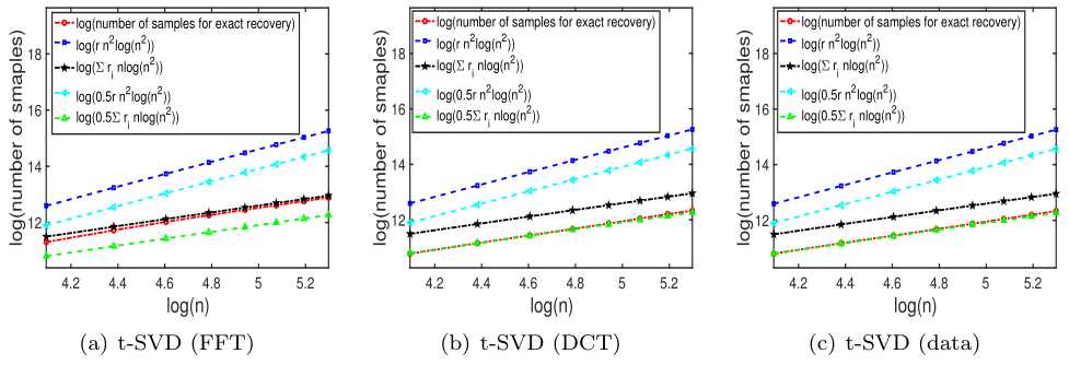
(a) t-SVD (FFT)

Figure 1: The number of samples of exact recovery, the sample sizes required by the right hand sides of (31) and (32) for different values of $n$ with $\sum_{i=1}^{n}r_{i}=200$.

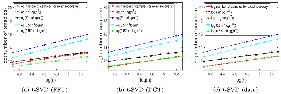
Figure 2: The number of samples of exact recovery, the sample sizes required by the right hand sides of (31) and (32) for different values of $n$ with $\sum_{i=1}^{n}r_{i}=300$.

In Figures 2 and 2, we test different values of $n$ (from 60 to 200 with the increment size being 20). The exact recovery means that five trials are tested and all of the relative errors are less than or equal to $10^{-2}$ in the experiments. We test constant₁, constant₂ = 0.5 or 1 in the right hand sides of (31) and (32) respectively to check how the theoretical bounds of sample sizes match with the actual number of samples for different values of $n$. It can be seen from Figures 2 and 2 that the curve $\sum_{i=1}^{n}r_{i}n\log(n^{2})$ based on the proposed bound with constant${}_{1}=1$ is close to the curve for the number of samples required by using t-SVD (FFT), and the curves $0.5\sum_{i=1}^{n}r_{i}n\log(n^{2})$ based on the proposed bound with constant${}_{1}=0.5$ is close to the curves for the number of samples required by using t-SVD (DCT) and t-SVD (data). Note that the corresponding slope of these lines in Figures 2 and 2 is equal to 1 derived by the $n$ term. In contrast, the curves constant${}_{2}rn^{2}\log(n^{2})$ based on the results in [42] do not fit the curves for the number of samples required by using t-SVD (FFT), t-SVD (DCT) and t-SVD (data), see the curves with constant${}_{2}=0.5,1$ in Figures 2 and 2. The main reason is that the corresponding slope of the lines in Figures 2 and 2 is equal to 2 derived by the $n^{2}$ term. According to Figures 2 and 2, we find that the theoretical bounds of sample sizes requirements in Theorem 3.1 match with the actual number of sample sizes for recovery.

4.2.2 Hyperspectral Images

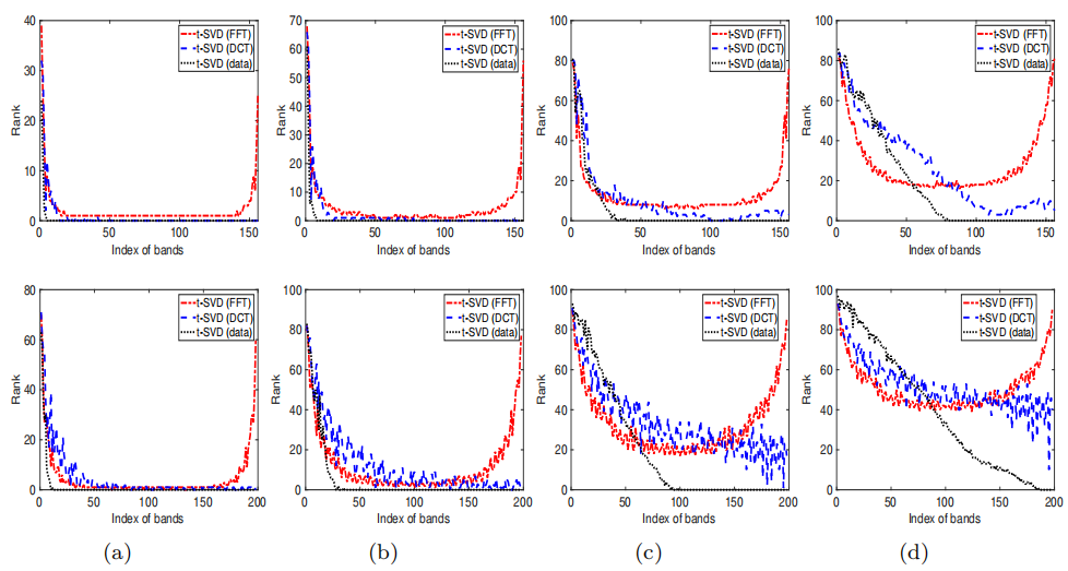
Figure 3: The distribution of transformed multi-ranks of the hyperspectral data sets with different truncations in each band. First row: Samson data set. Second row: Japser Ridge data set. (a) $\varpi=70\%$. (b) $\varpi=80\%$. (c) $\varpi=90\%$. (d) $\varpi=95\%$.

In this subsection, two hyperspectral data sets (Samson ($95\times 95\times 156$) and Japser Ridge ($100\times 100\times 198$) [43]) are used to demonstrate the required number of samples for tensor recovery by the proposed bound. For Samson data, $n_{1}$ and $n_{2}$ are equal to 95 and $n_{3}$ is equal to 156. For Japser Ridge data, $n_{1}$ and $n_{2}$ are equal to 100 and $n_{3}$ is equal to 198. Here we compare our method with the low-rank tensor completion method using the sum of nuclear norms of unfolding matrices of a tensor (LRTC) [12, 20], tensor factorization method (TF) [14], Square Deal [24], gradient descent algorithm on Grassmannians (GoG) [37]. These testing hyperspectral data is normalized on $[0,1]$. Their theoretical estimation of samples required are presented in Table 1.

We remark that these hyperspectral images are not exactly low multi-rank tensors, the multi-rank ($\sum_{i=1}^{n_{3}}r_{i}$) is not available. A truncated tensor is used to compute the transformed multi-rank and tubal rank by using the threshold $\varpi$. Here for a given tensor $\mathcal{Z}$ with transformed tensor SVD in (2) of Theorem 2.2 and $\varpi$, we determine the smallest value $k$ such that

$$\frac{\sum_{i=1}^{k}\varrho_{i}}{\sum_{i=1}^{n_{(2)}n_{3}}\varrho_{i}}\geq\varpi,$$

where $\{\varrho_{i}\}$ is the sorted value in ascending order of the numbers $\{(\hat{{\cal S}}_{\bf\Phi})_{jj\ell}\}_{1\leq j\leq n_{(2)},1\leq\ell\leq n_{3}}$ appearing in the diagonal tensor ${\cal S}$ in (2). The ratio is used to determine the significant numbers are kept in the truncated tensor based on the threshold $\varpi$. Now we can define the transformed multi-rank $\mathbf{r}(\varpi)$ of the truncated tensor as follows:

$$\mathbf{r}(\varpi):=(r_{1}(\varpi),\ldots,r_{n_{3}}(\varpi)),\ \mbox{with}\ r_{\ell}(\varpi):=\#\{(\hat{{\cal S}}_{\bf\Phi})_{jj\ell}\geq\varrho_{k},1\leq j\leq n_{(2)}\},\ \ell=1,\ldots,n_{3},$$

Accordingly, the transformed tubal rank of the truncated tensor is defined as $r(\varpi):=\max\{r_{1}(\varpi),\ldots,r_{n_{3}}(\varpi)\}$. The distributions of the transformed multi-ranks of the two hyperspectral data sets with different $\varpi$ are shown in Figure 3. It can be seen that the $\sum_{i=1}^{n_{3}}r_{i}(\varpi)$ obtained by t-SVD (data) is much smaller than that obtained by t-SVD (FFT) and t-SVD (DCT) for different truncations $\varpi=70\%,80\%,90\%,95\%$, which implies that the t-SVD (data) needs lower number of samples for successful recovery than t-SVD (FFT) and t-SVD (DCT). The distributions of the transformed multi-ranks of the truncated tensor obtained by t-SVD (FFT) are symmetric due to symmetry of FFT.

Table 2: The PSNR, SSIM values, and CPU time (in seconds) of different methods for the hyperspectral images.

Samson const₁ 20 30 40 50 60 70 80 sampling 0.013 0.019 0.026 0.032 0.039 0.045 0.052 rate LRTC PSNR 13.08 16.00 18.34 19.82 20.99 22.12 22.98 SSIM 0.3254 0.5720 0.6223 0.6643 0.6964 0.7287 0.7548 CPU 26.44 29.81 29.50 27.13 25.50 26.35 28.66 TF PSNR 4.05 7.45 20.26 29.78 32.86 35.54 36.39 SSIM 0.3990 0.4852 0.7798 0.8627 0.8856 0.9334 0.9440 CPU 207.55 207.20 206.90 206.80 216.99 210.21 207.86 Square Deal PSNR 16.35 18.55 20.38 22.15 23.77 25.57 26.77 SSIM 0.4502 0.5727 0.6696 0.7269 0.7916 0.8310 0.8667 CPU 37.46 34.93 33.05 30.96 29.48 29.63 34.05 GoG PSNR 16.72 26.02 27.13 30.01 30.45 30.87 31.43 SSIM 0.4851 0.6978 0.7560 0.8372 0.8366 0.8398 0.8665 CPU 1.05e4 1.40e4 3.41e4 3.87e4 4.61e4 3.46e4 4.15e4 t-SVD (FFT) PSNR 22.09 23.88 25.21 26.27 27.09 27.68 28.52 SSIM 0.5743 0.6498 0.6996 0.7442 0.7689 0.7912 0.8107 CPU 30.24 26.30 25.11 24.07 22.45 23.62 26.58 t-SVD (DCT) PSNR 26.35 28.72 30.42 31.92 33.03 33.96 35.04 SSIM 0.7355 0.8098 0.8552 0.8875 0.9096 0.9215 0.9343 CPU 172.41 167.56 177.44 185.69 193.36 187.29 190.13 t-SVD (data) PSNR 28.24 31.37 33.39 35.25 36.53 37.09 38.62 SSIM 0.8324 0.8971 0.9311 0.9539 0.9643 0.9658 0.9746 CPU 241.48 258.86 270.17 282.82 284.68 263.78 291.26 Japser Ridge const₁ 20 30 40 50 60 70 80 sampling 0.010 0.015 0.020 0.025 0.030 0.035 0.040 rate LRTC PSNR 12.48 14.80 16.78 18.17 18.97 19.61 20.15 SSIM 0.3245 0.4104 0.4404 0.4611 0.4793 0.5011 0.5223 CPU 39.54 39.98 42.73 39.81 36.51 40.21 42.36 TF PSNR 7.12 11.41 12.09 15.39 27.03 27.83 28.07 SSIM 0.2076 0.3728 0.6120 0.6418 0.7246 0.7603 0.7693 CPU 400.27 399.79 398.94 398.46 286.83 362.15 384.52 Square Deal PSNR 15.38 17.50 20.47 22.48 24.25 26.13 27.12 SSIM 0.3890 0.5168 0.6199 0.7021 0.7596 0.8046 0.8378 CPU 43.33 41.89 41.82 41.99 40.65 42.59 40.99 GoG PSNR 15.32 22.38 23.54 24.35 25.44 25.90 26.35 SSIM 0.2643 0.5430 0.5624 0.5835 0.6550 0.6808 0.7193 CPU 3.49e4 4.13e4 5.33e4 5.50e4 5.58e4 5.39e4 5.41e4 t-SVD (FFT) PSNR 21.04 22.95 24.09 25.17 26.06 26.74 27.25 SSIM 0.4877 0.5802 0.6353 0.6891 0.7270 0.7578 0.7756 CPU 50.54 42.01 37.62 35.38 34.36 42.69 35.99 t-SVD (DCT) PSNR 21.93 23.40 24.48 25.49 26.36 27.06 27.65 SSIM 0.5206 0.5945 0.6481 0.7015 0.7378 0.7647 0.7892 CPU 200.90 171.96 164.15 169.65 172.05 184.23 193.06 t-SVD (data) PSNR 23.54 25.63 27.47 28.74 30.09 30.78 31.33 SSIM 0.6004 0.7041 0.7816 0.8323 0.8675 0.8777 0.8962 CPU 235.74 217.07 217.13 230.64 235.28 225.95 231.87

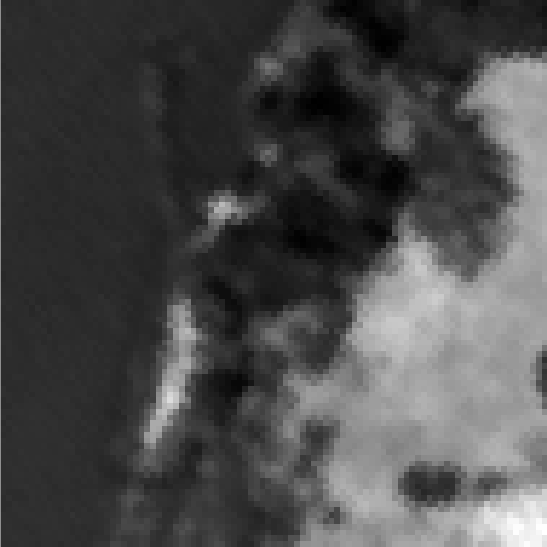
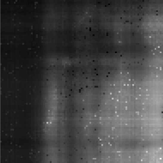
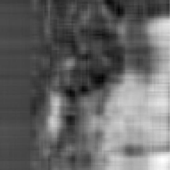
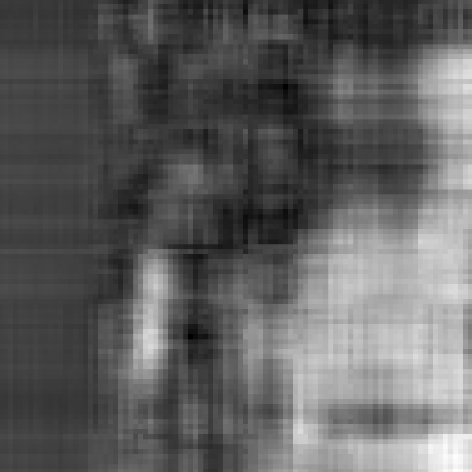
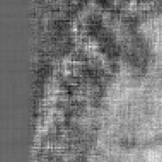
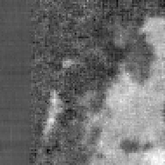
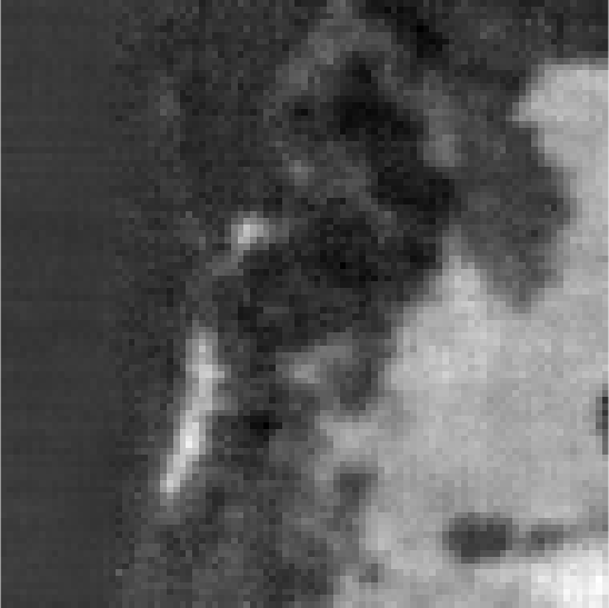
(a) 15th band

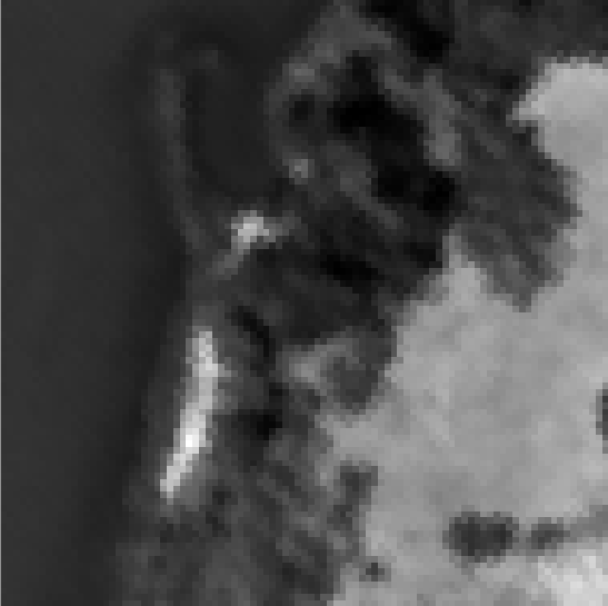
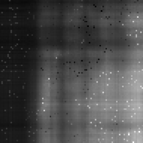
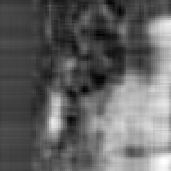
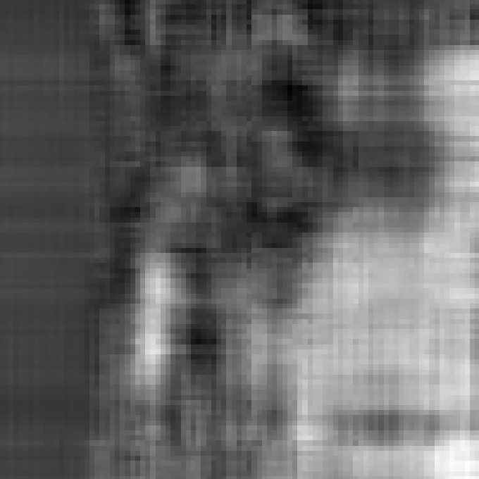
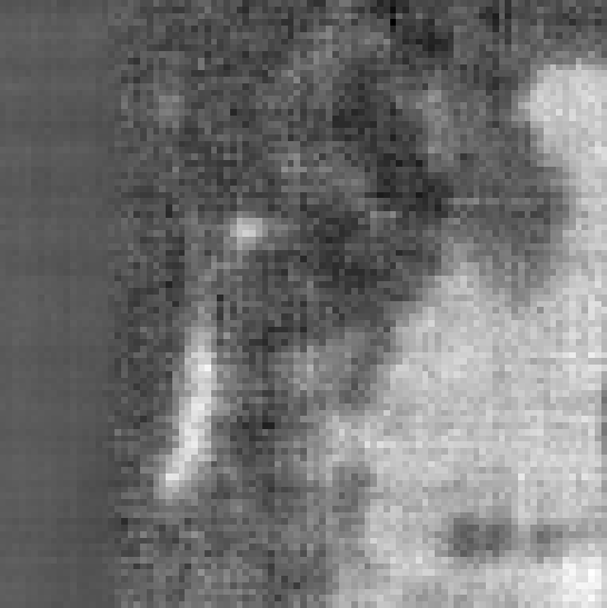
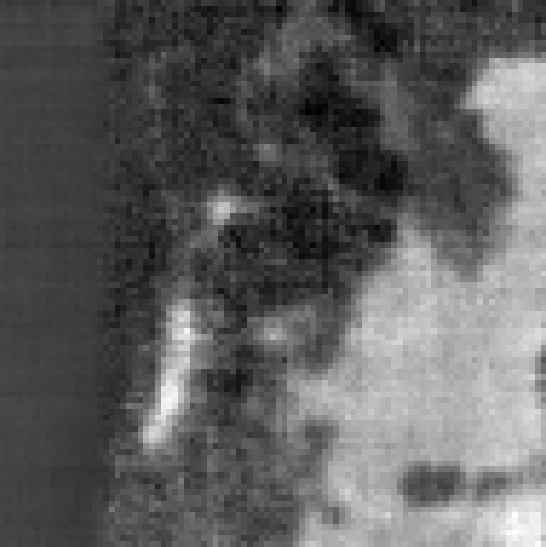
(b) 60th band

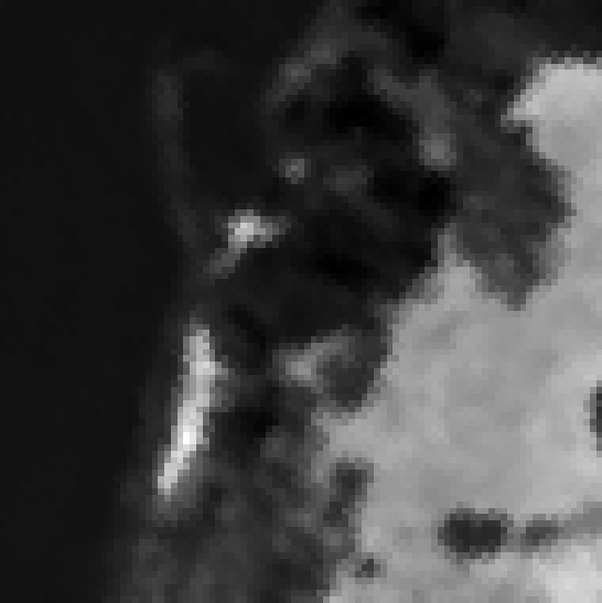
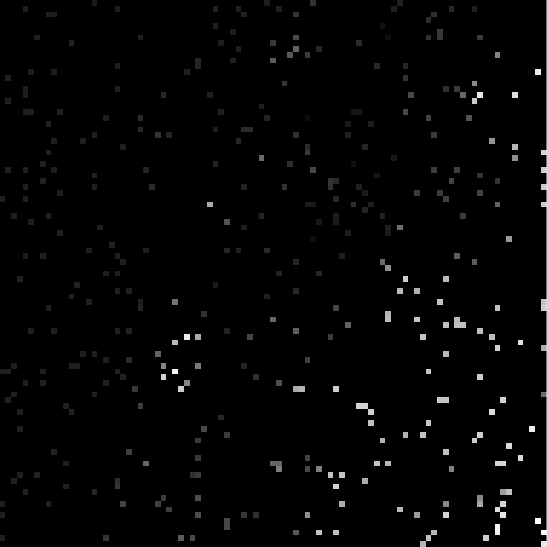
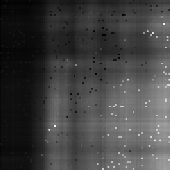
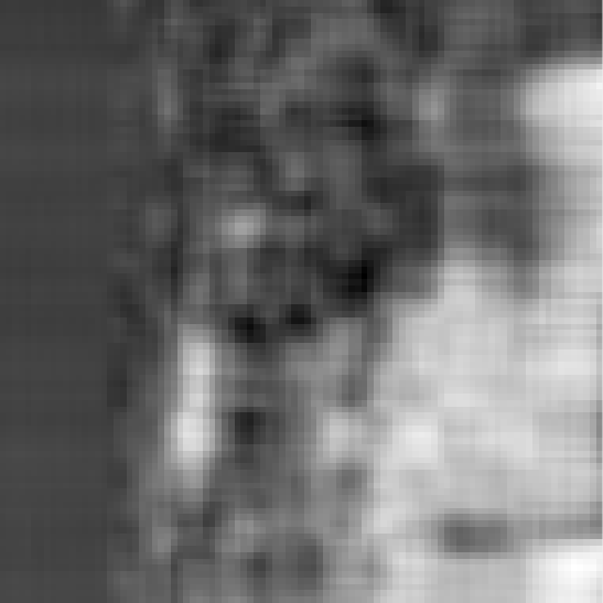
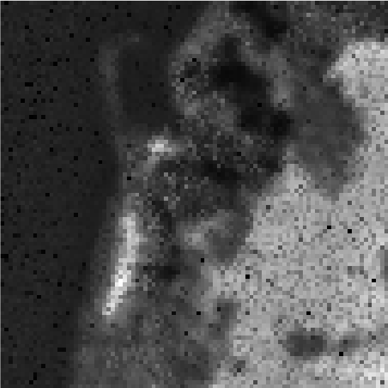
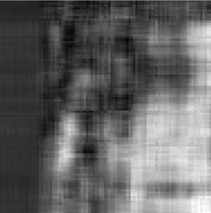
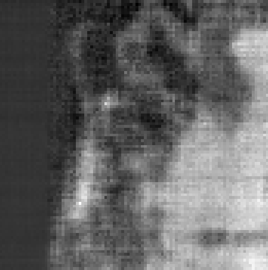
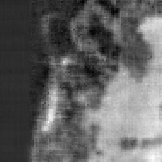
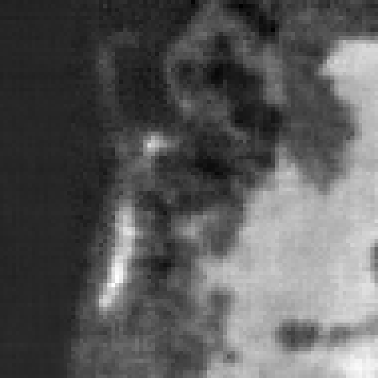
(c) 90th band

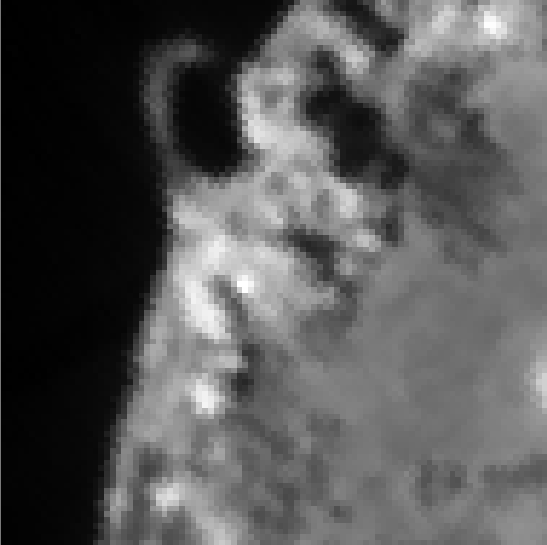
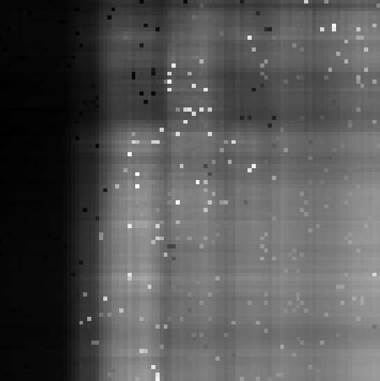
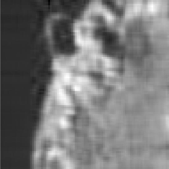
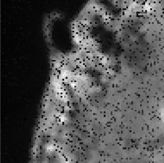
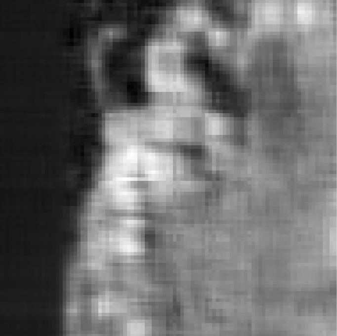
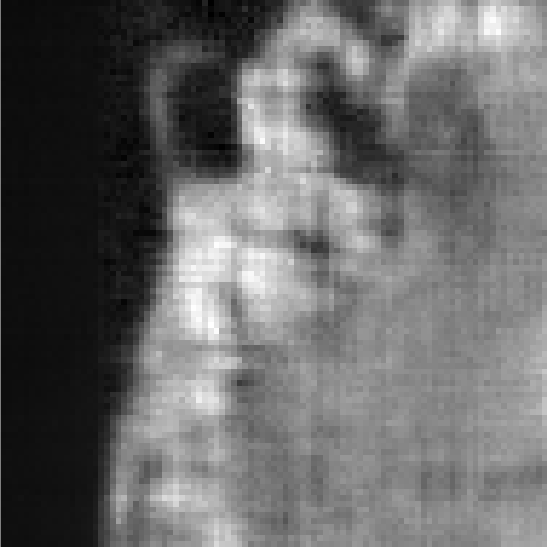
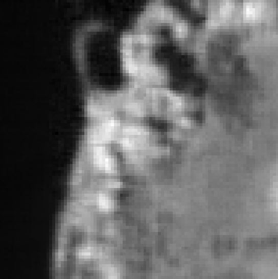
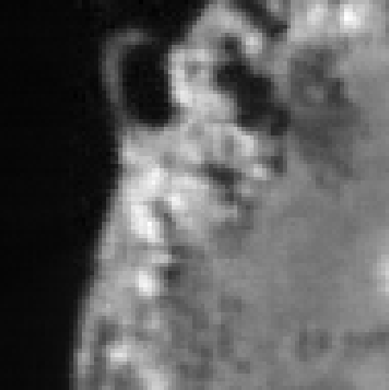
(d) 130th band

Figure 4: Recovery results by different methods for the Samson data with const${}_{1}=60$. First row: Original images. Second row: Observed images. Third row: Recovered images by LRTC. Fourth row: Recovered images by TF. Fifth row: Recovered images by Square Deal. Sixth row: Recovered images by GoG. Seventh row: Recovered images by t-SVD (FFT). Eighth row: Recovered images by t-SVD (DCT). Ninth row: Recovered images by t-SVD (data).

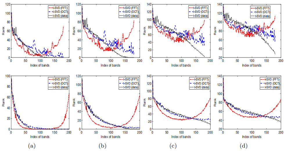
Figure 5: The distribution of transformed multi-ranks of the video data sets with different truncations in each frame. First row: Carphone data set. Second row: Announcer data set. (a) $\varpi=70\%$. (b) $\varpi=80\%$. (c) $\varpi=90\%$. (d) $\varpi=95\%$.

In Table 2, we present the number of samples (const${}_{1}n_{(1)}\log(n_{(1)}n_{3})$) for several values of const₁ and their corresponding PSNR and SSIM values of the recovered tensors by different methods, where const₁ varies from 20 to 80 with step-size $10$. Here we can regard const₁ as $c_{0}\mu\sum_{i=1}^{n_{3}}r_{i}(\varpi)$ in (10) of Theorem 3.1. For $\varpi=70\%$, the values $\sum_{i=1}^{n_{3}}r_{i}(\varpi)$ of Samson hyperspectral image are $346$, $129$, $40$ for t-SVD (FFT), t-SVD (DCT), and t-SVD (data), respectively. Thus, the chosen const₁ is proportional to $\sum_{i=1}^{n_{3}}r_{i}(\varpi)$ for the testing tensor of hyperspectral image with approximately low transformed multi-rank. We can see from the table that for different values of const₁, the PSNR and SSIM values obtained by t-SVD (data) and t-SVD (DCT) are higher than those obtained by LRTC, TF, Square Deal, GoG, and t-SVD (FFT). Moreover, when const${}_{1}=60$, the recovery performance of the t-SVD (FFT), t-SVD (DCT), and t-SVD (data) is good enough in terms of PSNR and SSIM values, which implies the number of sizes is enough for successful recovery by Theorem 3.1. When const₁ is larger, e.g., const${}_{1}=70,80$, the improvements of PSNR values of the t-SVD (FFT), t-SVD (DCT), and t-SVD (data) are smaller than those of other small const₁. For Samson data, the performance of GoG is better than that of t-SVD (FFT) for const${}_{1}\geq 30$. But the computational time required by GoG is significantly more than that required by the other methods. For Japser Ridge data, the PSNR and SSIM values obtained by all three t-SVD methods are almost higher than those obtained by LRTC, TF, Square Deal, and GoG. Moreover, the computational time required by the t-SVD methods are quite efficient compared with the other methods.

Figure 4 shows the visual comparisons of different bands obtained by LRTC, TF, Square Deal, GoG, and three t-SVD methods for the Samson data, where const${}_{1}=60$. We can see that the t-SVD (data) and t-SVD (DCT) outperform LRTC, TF, Square Deal, and t-SVD (FFT) in terms of visual quality. Moreover, the images recovered by t-SVD (data) keep more details than those recovered by LRTC, TF, Square Deal, t-SVD (FFT), and t-SVD (DCT).

4.2.3 Video Data

In this subsection, we test two video data sets (length $\times$ width $\times$ frames) to show the performance of the proposed method, where the testing videos include Carphone ($144\times 176\times 180$) and Announcer ($144\times 176\times 200$), and we just use the first channels of all frames in the original data. Moreover, the first $180$ and $200$ frames for the two videos are chosen to improve the computational time. The intensity range of the video images is scaled into $[0,1]$ in the experiments.

Table 3: The PSNR, SSIM values, and CPU time (in seconds) of different methods for the video data sets.

const₁ 20 30 40 50 60 70 80 90 100 110 120 sampling 0.008 0.012 0.016 0.020 0.024 0.028 0.032 0.036 0.040 0.044 0.048 rate Carphone LRTC PSNR 10.81 11.65 12.49 13.19 13.97 14.75 15.40 16.01 16.53 17.05 17.52 SSIM 0.3498 0.3571 0.3687 0.3870 0.4085 0.4319 0.4496 0.4701 0.4862 0.5038 0.5206 CPU 90.78 85.06 85.92 85.12 89.76 92.28 91.70 90.47 92.91 92.06 95.21 TF PSNR 4.96 4.64 13.41 12.98 20.82 22.57 22.66 22.74 22.75 22.85 23.04 SSIM 0.2855 0.4507 0.5081 0.5499 0.5837 0.6461 0.6531 0.6607 0.6622 0.6705 0.6746 CPU 780.55 779.63 771.43 782.11 762.25 770.57 771.03 765.42 760.32 782.45 795.41 Square Deal PSNR 10.04 12.99 13.55 15.00 16.98 17.15 18.10 19.15 20.42 20.47 21.17 SSIM 0.1796 0.2675 0.3304 0.3988 0.4497 0.4930 0.5348 0.5719 0.6113 0.6178 0.6396 CPU 76.98 80.23 76.06 77.03 76.76 76.36 74.78 80.00 78.59 77.21 79.75 GoG PSNR 18.59 20.18 20.77 20.46 21.22 21.35 21.48 22.11 22.47 22.86 23.15 SSIM 0.4010 0.4653 0.5229 0.5023 0.5449 0.5483 0.5547 0.5768 0.5874 0.5936 0.6058 CPU 1.09e5 2.27e5 1.30e5 1.40e5 2.47e5 6.27e5 3.76e5 6.71e5 6.32e5 6.52e5 6.48e5 t-SVD (FFT) PSNR 9.79 11.55 15.06 18.53 22.04 22.59 23.07 23.38 23.72 24.01 24.24 SSIM 0.1814 0.2463 0.3759 0.4899 0.6121 0.6367 0.6566 0.6690 0.6816 0.6934 0.7017 CPU 53.78 58.69 77.43 88.78 107.26 103.15 98.25 93.03 88.88 90.36 92.81 t-SVD (DCT) PSNR 20.24 21.18 21.93 22.42 22.91 23.24 23.60 23.87 24.15 24.44 24.65 SSIM 0.5230 0.5720 0.6044 0.6286 0.6506 0.6642 0.6772 0.6890 0.6484 0.7106 0.7185 CPU 323.11 291.24 271.55 251.17 237.77 226.54 214.85 205.35 198.58 200.15 197.32 t-SVD (data) PSNR 20.39 21.43 22.30 22.87 23.45 23.75 24.23 24.56 24.85 24.94 25.17 SSIM 0.5294 0.5841 0.6236 0.6499 0.6747 0.6877 0.7063 0.7200 0.7298 0.7329 0.7426 CPU 366.20 337.21 314.40 293.42 278.06 261.55 253.14 242.91 235.86 261.02 248.59 const₁ 20 30 40 50 60 70 80 90 100 110 120 sampling 0.007 0.011 0.015 0.018 0.022 0.025 0.029 0.033 0.036 0.040 0.044 rate Announcer LRTC PSNR 12.72 14.03 15.28 16.42 17.76 18.83 19.88 20.74 21.46 22.06 22.58 SSIM 0.4727 0.4900 0.5087 0.5336 0.5601 0.5869 0.6120 0.6341 0.6520 0.6710 0.6871 CPU 100.75 96.25 100.67 103.05 104.02 105.00 104.68 103.02 100.29 101.23 100.96 TF PSNR 4.39 9.99 11.36 15.48 24.12 25.65 26.22 26.28 27.99 28.29 28.34 SSIM 0.4229 0.6176 0.6599 0.6743 0.7076 0.7363 0.7534 0.7544 0.8169 0.8265 0.8300 CPU 887.20 862.11 872.41 874.64 869.01 864.04 822.11 835.96 858.93 862.62 839.15 Square Deal PSNR 11.50 14.61 16.71 19.36 20.86 23.34 24.15 24.27 26.76 28.24 28.87 SSIM 0.1692 0.2702 0.3780 0.5004 0.6207 0.6950 0.7488 0.7928 0.8394 0.8743 0.8918 CPU 86.39 87.33 80.39 78.26 77.23 77.46 80.36 80.28 81.06 80.25 80.38 GoG PSNR 21.85 23.59 23.72 24.80 24.96 25.42 26.20 26.87 27.14 27.43 27.79 SSIM 0.5113 0.5854 0.6144 0.6691 0.6775 0.6976 0.7183 0.7566 0.7977 0.8236 0.8395 CPU 1.94e5 2.31e5 2.60e5 3.54e5 6.09e5 6.36e5 5.49e5 5.98e5 5.90e5 5.89e5 6.01e5 t-SVD (FFT) PSNR 11.01 16.64 27.03 27.98 28.63 29.11 29.46 29.83 30.12 30.35 30.62 SSIM 0.2606 0.5339 0.8125 0.8380 0.8564 0.8686 0.8776 0.8865 0.8922 0.8987 0.9022 CPU 61.87 97.82 153.63 144.82 132.18 125.67 118.75 106.63 103.44 113.25 108.63 t-SVD (DCT) PSNR 26.06 27.12 27.92 28.58 29.16 29.58 29.95 30.32 30.69 30.93 31.17 SSIM 0.7645 0.8078 0.8353 0.8875 0.8703 0.8798 0.8893 0.8985 0.9046 0.9099 0.9140 CPU 537.80 466.05 432.45 407.57 377.23 350.59 329.40 298.93 287.79 298.46 284.32 t-SVD (data) PSNR 26.08 27.25 28.12 28.76 29.41 29.88 30.24 30.71 31.14 31.29 31.58 SSIM 0.7649 0.8113 0.8399 0.8581 0.8741 0.8838 0.8941 0.9037 0.9106 0.9150 0.9198 CPU 608.38 531.39 472.35 460.30 425.59 395.42 353.94 341.43 330.40 365.25 341.29

Similar to Section 4.2.2, the video data sets are not exactly low-rank. First, we show the distributions of the transformed multi-ranks with different transformations and truncations $\varpi$ in Figure 5. It can be observed that the $\sum_{i=1}^{n_{3}}r_{i}(\varpi)$ obtained by t-SVD (data) is much smaller than that obtained by t-SVD (FFT) and t-SVD (DCT) for different $\varpi$. Therefore, the number of samples required by t-SVD (data) would be smaller than that required by t-SVD (FFT) and t-SVD (DCT) for the same performance. The distributions of transformed multi-ranks obtained by t-SVD (FFT) are symmetric for different $\varpi$ since the FFT has symmetric property.

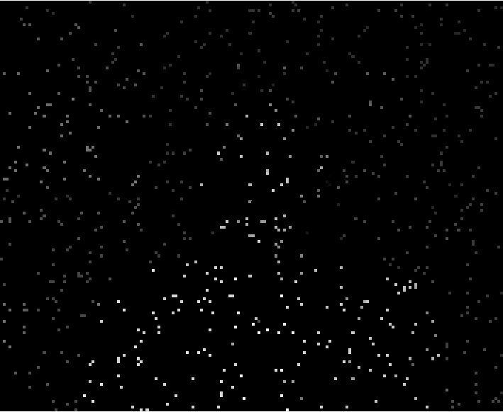
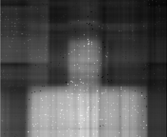
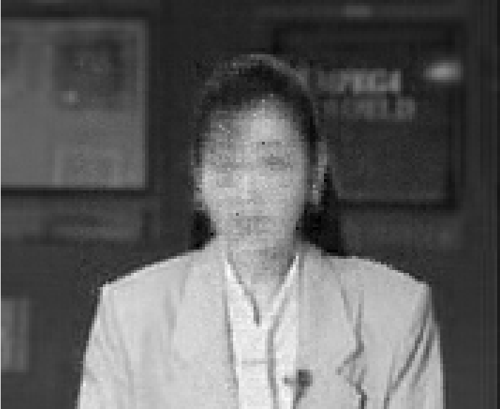
(a) 20th frame

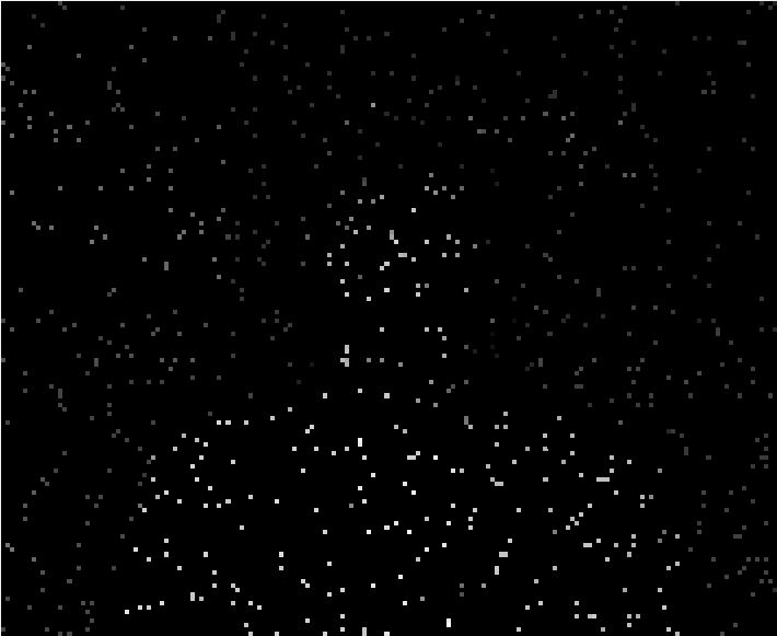
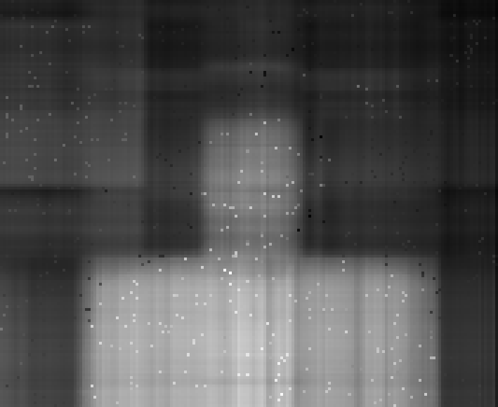
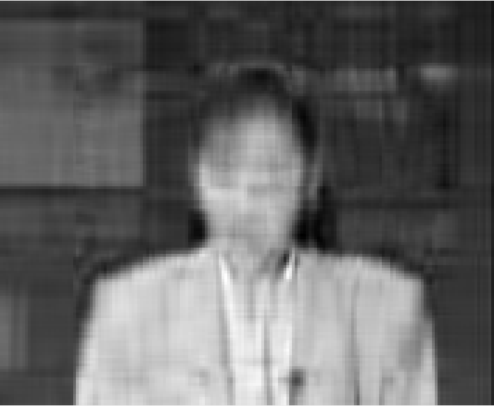
(b) 80th frame

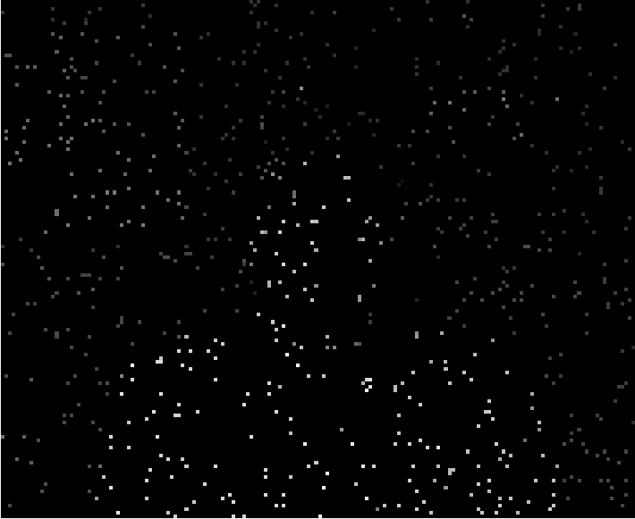
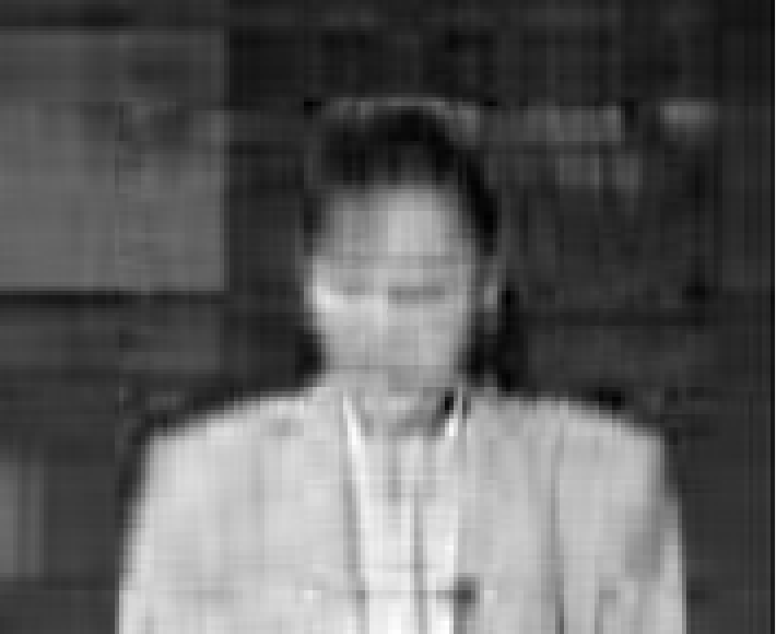
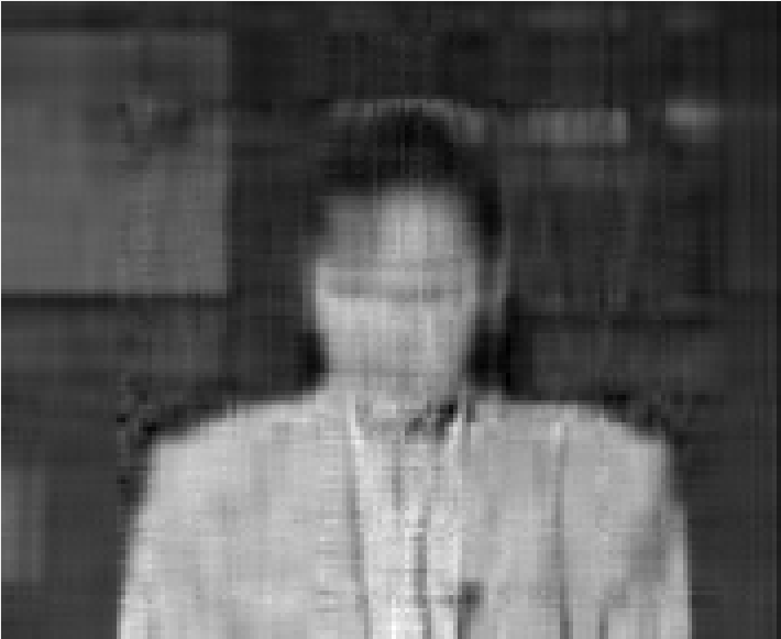
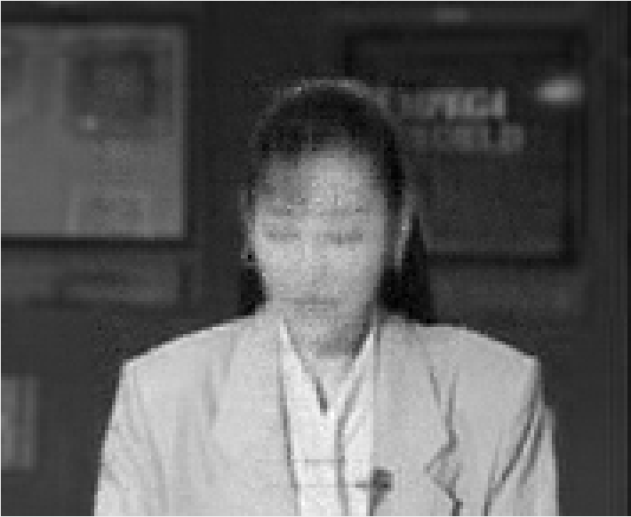
(c) 120th frame

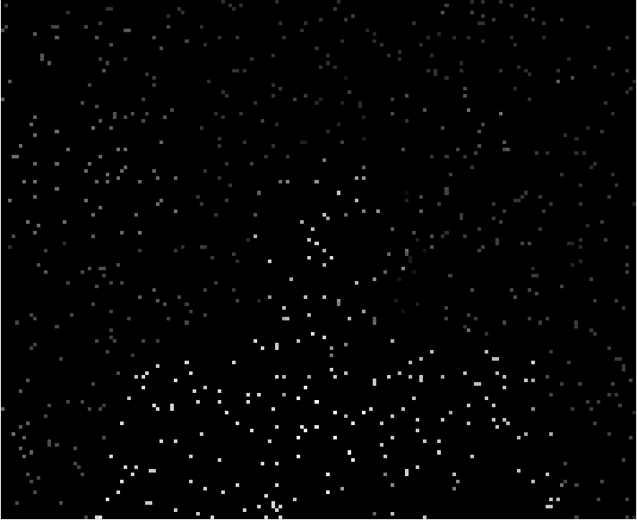
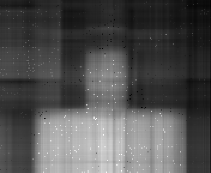
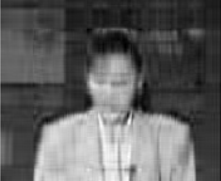
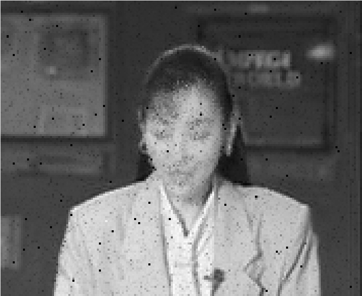
(d) 180th frame

Figure 6: Recovery results by different methods for the Announcer data with const${}_{1}=80$. First row: Original images. Second row: Observed images. Third row: Recovered images by LRTC. Fourth row: Recovered images by TF. Fifth row: Recovered images by Square Deal. Sixth row: Recovered images by GoG. Seventh row: Recovered images by t-SVD (FFT). Eighth row: Recovered images by t-SVD (DCT). Ninth row: Recovered images by t-SVD (data).

We use const${}_{1}n_{(1)}\log(n_{(1)}n_{3})$ number of samples based on Theorem 3.1. The range const₁ is from 20 to 120 with increment step-size being 10. For example, when $\varpi=70\%$, the $\sum_{i=1}^{n_{3}}r_{i}(\varpi)$ of Announcer obtained by t-SVD (FFT), t-SVD (DCT), t-SVD (data) are $1886$, $1649$, $1502$, respectively. When const₁ is equal to 100, the required sample size would be enough for successful recovery by Theorem 3.1. When const${}_{1}>100$, e.g., const${}_{1}=110,120$, the improvements of PSNR values by the three t-SVD methods are very small. In Table 3, we show the PSNR, SSIM values, and CPU time (in seconds) of different methods for the testing video data sets with different const₁. It can be seen that the performance of t-SVD (data) is better than that of LRTC, TF, Square Deal, GoG, t-SVD (FFT), and t-SVD (DCT) in terms of PSNR and SSIM values. The PSNR and SSIM values obtained by t-SVD (DCT) are higher than those obtained by t-SVD (FFT). Hence, the number of samples required by t-SVD (DCT) and t-SVD (data) is smaller than that required by LRTC, TF, Square Deal, GoG, and t-SVD (FFT) for the same recovery performance, which demonstrates the conclusion of Theorem 3.1. Moreover, the CPU time (in seconds) required by GoG is much more than that required by other methods.

Figure 6 shows the visual quality of the 20th, 80th, 120th, 180th frames of the recovered images by LRTC, TF, Square Deal, GoG, and three t-SVD methods, where const${}_{1}=80$. It can be seen that the three t-SVD methods outperform LRTC, TF, Square Deal, and GoG for different frames in terms of visual quality, where the recovered images by the t-SVD methods are more clear.

5 Concluding Remarks

In this paper, we have established the sample size requirement for exact recovery in the tensor completion problem by using transformed tensor SVD. We have shown that for any $\mathcal{Z}\in\mathbb{C}^{n_{1}\times n_{2}\times n_{3}}$ with transformed multi-rank $(r_{1},r_{2},\ldots,r_{n_{3}})$, one can recover the tensor exactly with high probability under some incoherence conditions if the sample size of observations is of the order $O(\sum_{i=1}^{n_{3}}r_{i}\max\{n_{1},n_{2}\}\log(\max\{n_{1},n_{2}\}n_{3}))$ under uniformly sampled entries. The sample size requirement of our theory for exact recovery is smaller than that of existing methods for tensor completion. Moreover, several numerical experiments on both synthetic data and real-world data sets are presented to show the superior performance of our methods in comparison with other state-of-the-art methods.

In further work, it would be of great interest to extend the transformed tensor SVD and tensor completion results to higher-order tensors (cf. [22]). It would be also of great interest to extend the result of the unitary transformation to any invertible linear transformation for tensor completion (cf. [15]).

Appendix A.

We first list the following lemma, which is the main tool to prove our conclusions.

Lemma 5.1.

([28, Theorem 4]) Let $X_{1},\ldots,X_{L}\in\mathbb{R}^{n\times n}$ be independent zero mean random matrices of dimension $d_{1}\times d_{2}$. Suppose $\rho_{k}^{2}=\max\left\{\|\mathbb{E}[X_{k}X_{k}^{T}]\|,\|\mathbb{E}[X_{k}^{T}X_{k}]\|\right\}$ and $\|X_{k}\|\leq B$ almost surely for all $k=1,\ldots,L.$ Then for any $\tau>0,$

$$\mathbb{P}\left[\Biggl{\|}\sum_{k=1}^{L}X_{k}\Biggl{\|}>\tau\right]\leq(d_{1}+d_{2})\exp\left(\frac{-\tau^{2}/2}{\sum_{k=1}^{L}\rho_{k}^{2}+B\tau/3}\right).$$

Moreover, if $\max\left\{\big{\|}\sum_{k=1}^{L}X_{k}X_{k}^{T}\big{\|},\big{\|}\sum_{k=1}^{L}X_{k}^{T}X_{k}\big{\|}\right\}\leq\sigma^{2},$ then for any $c>1,$ we have

$$\left\|\sum_{k=1}^{L}X_{k}\right\|\leq\sqrt{4c\sigma^{2}\log(d_{1}+d_{2})}+cB\log(d_{1}+d_{2})$$

holds with probability at least $1-(d_{1}+d_{2})^{-(c-1)}.$

Proof of Lemma 3.3

Let $\mathcal{E}_{ijk}$ be a unit tensor whose $(i,j,k)$-th entry is 1 and others are 0. Then for an arbitrary tensor $\mathcal{Z}\in\mathbb{C}^{n_{1}\times n_{2}\times n_{3}}$, we have $\mathcal{Z}=\sum_{i,j,k}\langle\mathcal{E}_{ijk},\mathcal{Z}\rangle\mathcal{E}_{ijk}.$ Recall Definition 2.7, $\mathcal{E}_{ijk}$ can be expressed as $\mathcal{E}_{ijk}=\vec{\bm{e}}_{ik}\diamond_{\bf\Phi}\ddot{\bm{e}}_{k}\diamond_{\bf\Phi}\vec{\bm{e}}_{jk}^{H},$ then ${\cal P}_{T}(\mathcal{Z})$ can also be decomposed as

$${\cal P}_{T}(\mathcal{Z})=\sum_{i,j,k}\langle{\cal P}_{T}(\mathcal{Z}),\vec{\bm{e}}_{ik}\diamond_{\bf\Phi}\ddot{\bm{e}}_{k}\diamond_{\bf\Phi}\vec{\bm{e}}^{H}_{jk}\rangle\vec{\bm{e}}_{ik}\diamond_{\bf\Phi}\ddot{\bm{e}}_{k}\diamond_{\bf\Phi}\vec{\bm{e}}^{H}_{jk},$$

where $T$ is defined as (9). Similarly,

$$\rho^{-1}{\cal P}_{T}{\cal P}_{\Omega}{\cal P}_{T}(\mathcal{Z})=\sum_{i,j,k}\rho^{-1}\delta_{ijk}\langle\mathcal{Z},{\cal P}_{T}(\vec{\bm{e}}_{ik}\diamond_{\bf\Phi}\ddot{\bm{e}}_{k}\diamond_{\bf\Phi}\vec{\bm{e}}^{H}_{jk})\rangle{\cal P}_{T}(\vec{\bm{e}}_{ik}\diamond_{\bf\Phi}\ddot{\bm{e}}_{k}\diamond_{\bf\Phi}\vec{\bm{e}}^{H}_{jk}).$$

Define the operator $\mathcal{T}^{ijk}$ as:

$$\mathcal{T}^{ijk}(\mathcal{Z})=\rho^{-1}\delta_{ijk}\langle\mathcal{Z},{\cal P}_{T}(\vec{\bm{e}}_{ik}\diamond_{\bf\Phi}\ddot{\bm{e}}_{k}\diamond_{\bf\Phi}\vec{\bm{e}}^{H}_{jk})\rangle{\cal P}_{T}(\vec{\bm{e}}_{ik}\diamond_{\bf\Phi}\ddot{\bm{e}}_{k}\diamond_{\bf\Phi}\vec{\bm{e}}^{H}_{jk}).$$

Then by the definition of tensor operator norm, we can get

$$\|\mathcal{T}^{ijk}\|_{\textup{op}}=\frac{1}{\rho}\|{\cal P}_{T}(\vec{\bm{e}}_{ik}\diamond_{\bf\Phi}\ddot{\bm{e}}_{k}\diamond_{\bf\Phi}\vec{\bm{e}}^{H}_{jk})\|^{2}_{F},~{}\text{and}~{}\|{\cal P}_{T}\|_{\textup{op}}\leq 1.$$

Note the fact that for any two positive semidefinite matrices ${A},{B}\in\mathbb{C}^{n\times n}$, we have $\|{A}-{B}\|\leq\max\{\|{A}\|,\|{B}\|\}.$ Therefore, by the inequality given in Proposition 3.2, we have

$$\Big{\|}\mathcal{T}^{ijk}-\frac{1}{n_{1}n_{2}n_{3}}{\cal P}_{T}\Big{\|}_{\textup{op}}\leq\max\left\{\frac{1}{\rho}\|{\cal P}_{T}(\vec{\bm{e}}_{ik}\diamond_{\bf\Phi}\ddot{\bm{e}}_{k}\diamond_{\bf\Phi}\vec{\bm{e}}^{H}_{jk})\|^{2}_{F},\frac{1}{n_{1}n_{2}n_{3}}\right\}\leq\frac{2\mu\sum{r_{i}}}{n_{(2)}n_{3}\rho}.$$

In addition, one has

$$~{}\Big{\|}\mathbb{E}\Big{(}\mathcal{T}^{ijk}-\frac{1}{n_{1}n_{2}n_{3}}{\cal P}_{T}\Big{)}^{2}\Big{\|}_{\textup{op}}$$

$$\leq ~{}\left\|\mathbb{E}\left(\frac{1}{\rho}\|{\cal P}_{T}(\vec{\bm{e}}_{ik}\diamond_{\bf\Phi}\ddot{\bm{e}}_{k}\diamond_{\bf\Phi}\vec{\bm{e}}^{H}_{jk})\|^{2}_{F}\mathcal{T}^{ijk}\right)-\frac{2}{n_{1}n_{2}n_{3}}{\cal P}_{T}\mathbb{E}(\mathcal{T}^{ijk})+\frac{1}{n^{2}_{1}n^{2}_{2}n^{2}_{3}}{\cal P}_{T}\right\|$$

$$= ~{}\left\|\frac{1}{\rho}\|{\cal P}_{T}(\vec{\bm{e}}_{ik}\diamond_{\bf\Phi}\ddot{\bm{e}}_{k}\diamond_{\bf\Phi}\vec{\bm{e}}^{H}_{jk})\|^{2}_{F}\frac{1}{n_{1}n_{2}n_{3}}{\cal P}_{T}-\frac{1}{n^{2}_{1}n^{2}_{2}n^{2}_{3}}{\cal P}_{T}\right\|\leq\frac{2\mu\sum{r_{i}}}{n_{(1)}n^{2}_{(2)}n^{2}_{3}\rho}.$$

Setting $\tau=\sqrt{\frac{14\mu\beta\sum{r_{i}}\log(n_{(1)}n_{3})}{3n_{(2)}n_{3}\rho}}\leq\frac{1}{2}$ with any $\beta>1$ and using Lemma 5.1, we have

$$\mathbb{P}[\|\rho^{-1}{\cal P}_{T}{\cal P}_{\Omega}{\cal P}_{T}-{\cal P}_{T}\|_{\textup{op}}>\tau]=\mathbb{P}\left[\left\|\sum_{i,j,k}\left(\mathcal{T}^{ijk}-\frac{1}{n_{1}n_{2}n_{3}}{\cal P}_{T}\right)\right\|_{\textup{op}}>\tau\right]$$

$$\leq~{} 2n_{(1)}n_{3}\exp\Bigg{(}\frac{\frac{-7\mu\beta\sum{r_{i}}\log(n_{(1)}n_{3})}{3n_{(2)}n_{3}\rho}}{\frac{2\mu\sum{r_{i}}}{n_{(2)}n_{3}\rho}+\frac{2\mu\sum{r_{i}}}{6n_{(2)}n_{3}\rho}}\Bigg{)}=2n_{(1)}n_{3}\exp({-\beta\log n_{(1)}n_{3}})=2(n_{(1)}n_{3})^{1-\beta},$$

which implies that

$$\mathbb{P}\left[\|\rho^{-1}{\cal P}_{T}{\cal P}_{\Omega}{\cal P}_{T}-{\cal P}_{T}\|_{\textup{op}}\leq\epsilon\right]\geq 1-2(n_{(1)}n_{3})^{1-\beta}.$$

This completes the proof.

Appendix B. Proof of Lemma 3.4

Denote

$$\rho^{-1}\mathcal{P}_{\Omega}(\mathcal{Z})-\mathcal{Z}=\sum_{i,j,k}\mathcal{G}^{ijk}=\sum_{i,j,k}\Big{(}\frac{1}{\rho}\delta_{ijk}-1\Big{)}\mathcal{Z}_{ijk}\vec{\bm{e}}_{ik}\diamond_{\bf\Phi}\ddot{\bm{e}}_{k}\diamond_{\bf\Phi}\vec{\bm{e}}^{H}_{jk}.$$

Then by the independence of $\delta_{ijk}$, we have $\mathbb{E}[\mathcal{G}^{ijk}]=\bf{0}$ and $\|\mathcal{G}^{ijk}\|\leq\frac{1}{\rho}\|\mathcal{Z}\|_{\infty}.$ Moreover,

$$\left\|\mathbb{E}\left[\sum_{i,j,k}(\mathcal{G}^{ijk})^{H}\diamond_{\bf\Phi}\mathcal{G}^{ijk}\right]\right\| =\left\|\sum_{i,j,k}|\mathcal{Z}_{ijk}|^{2}\vec{\bm{e}}_{jk}\diamond_{\bf\Phi}\vec{\bm{e}}_{jk}^{H}\mathbb{E}\left(\frac{1}{\rho}\delta_{ijk}-1\right)^{2}\right\|$$

$$=\left\|\frac{1-\rho}{\rho}\sum_{i,j,k}|\mathcal{Z}_{ijk}|^{2}\vec{\bm{e}}_{ik}\diamond_{\bf\Phi}\vec{\bm{e}}_{ik}^{H}\right\|.$$

Recall the definition of tensor basis, we can get that ${\bf\Phi}[\vec{\bm{e}}_{jk}\diamond_{\bf\Phi}\vec{\bm{e}}_{jk}^{H}]$ is a tensor except the $(j,j,t)$-th tube entries equaling to $({\bf\Phi}[\mathring{\bm{e}}_{k}])_{t}^{2}=\alpha^{2}_{t},t=1,\ldots,n_{3}$ with $\sum_{t=1}^{n_{3}}\alpha_{t}^{2}=1,$ and 0 otherwise. Hence, we get that

$$\left\|\mathbb{E}\left[\sum_{i,j,k}(\mathcal{G}^{ijk})^{H}\diamond_{\bf\Phi}\mathcal{G}^{ijk}\right]\right\| =\frac{1-\rho}{\rho}\left\|\sum_{i,j,k}|\mathcal{Z}_{ijk}|^{2}\vec{\bm{e}}_{jk}\diamond_{\bf\Phi}\vec{\bm{e}}_{jk}^{H}\right\|$$

$$=\frac{1-\rho}{\rho}\max_{j}\left\|\sum_{i,j,k}|\mathcal{Z}_{ijk}|^{2}\vec{\bm{e}}_{jk}\diamond_{\bf\Phi}\vec{\bm{e}}_{jk}^{H}\right\|$$

$$=\frac{1-\rho}{\rho}\max_{j}\left\|\sum_{i,k}|\mathcal{Z}_{ijk}|^{2}(\overline{\vec{\bm{e}}}_{jk})_{\bf\Phi}\cdot(\overline{\vec{\bm{e}}}_{jk})_{\bf\Phi}^{H}\right\|\leq\frac{1}{\rho}\|\mathcal{Z}\|^{2}_{\infty,w}.$$

Moreover, $\left\|\mathbb{E}\left[\sum_{i,j,k}\mathcal{G}^{ijk}\diamond_{\bf\Phi}(\mathcal{G}^{ijk})^{H}\right]\right\|$ can be also bounded similarly. Then by Lemma 5.1, we can get that

$$\|\rho^{-1}\mathcal{P}_{\Omega}(\mathcal{Z})-\mathcal{Z}\|_{\textup{op}}\leq c\left(\frac{\log(n_{(1)}n_{3})}{\rho}\|\mathcal{Z}\|_{\infty}+\sqrt{\frac{\log(n_{(1)}n_{3})}{\rho}}\|\mathcal{Z}\|_{\infty,w}\right)$$

holds with high probability provided that $m\geq C_{0}\epsilon^{-2}\mu\sum{r_{i}}n_{(1)}\log(n_{(1)}n_{3}).$

Appendix C. Proof of Lemma 3.5

Denote the weighted $b$-th lateral slice of $(\rho^{-1}\mathcal{P}_{T}\mathcal{P}_{\Omega}-\mathcal{P}_{T})\mathcal{Z}$ as

$$\sum_{i,j,k}\mathcal{F}^{ijk}: =(\rho^{-1}\mathcal{P}_{T}\mathcal{P}_{\Omega}-\mathcal{P}_{T})\mathcal{Z}\diamond_{\bf\Phi}\vec{\bm{e}}_{bk}$$

$$=\sum_{i,j,k}\Big{(}\frac{1}{\rho}\delta_{ijk}-1\Big{)}\mathcal{Z}_{ijk}\mathcal{P}_{T}(\vec{\bm{e}}_{ik}\diamond_{\bf\Phi}\ddot{\bm{e}}_{k}\diamond_{\bf\Phi}\vec{\bm{e}}^{H}_{jk})\diamond_{\bf\Phi}\vec{\bm{e}}_{bk},$$

where $\mathcal{F}^{ijk}\in\mathbb{C}^{n_{1}\times 1\times n_{3}}$ are zero-mean independent lateral slices. By the incoherence conditions given in Proposition 3.2, we have

$$\|\mathcal{F}^{ijk}\|_{{F}}=\left\|\left(\frac{1}{\rho}\delta_{ijk}-1\right)\mathcal{Z}_{ijk}\mathcal{P}_{T}(\vec{\bm{e}}_{ik}\diamond_{\bf\Phi}\ddot{\bm{e}}_{k}\diamond_{\bf\Phi}\vec{\bm{e}}^{H}_{jk})\diamond_{\bf\Phi}\vec{\bm{e}}_{bk}\right\|_{{F}}\leq\frac{1}{\rho}\sqrt{\frac{2\mu\sum_{i=1}^{n_{3}}r_{i}}{n_{1}n_{3}}}\|\mathcal{Z}\|_{\infty}.$$

Furthermore,

$$\left\|\mathbb{E}\left[\sum_{i,j,k}(\mathcal{F}^{ijk})^{H}\diamond_{\bf\Phi}\mathcal{F}^{ijk}\right]\right\|_{{F}}=\frac{1-\rho}{\rho}\sum_{i,j,k}|\mathcal{Z}_{ijk}|^{2}\|\mathcal{P}_{T}(\vec{\bm{e}}_{ik}\diamond_{\bf\Phi}\ddot{\bm{e}}_{k}\diamond_{\bf\Phi}\vec{\bm{e}}^{H}_{jk})\diamond_{\bf\Phi}\vec{\bm{e}}_{bk}\|^{2}_{{F}}.$$

Then by the definition of $\mathcal{P}_{T}$, we can get

$$~{}\|\mathcal{P}_{T}(\vec{\bm{e}}_{ik}\diamond_{\bf\Phi}\ddot{\bm{e}}_{k}\diamond_{\bf\Phi}\vec{\bm{e}}^{H}_{jk})\diamond_{\bf\Phi}\vec{\bm{e}}_{bk}\|^{2}_{F}$$

$$= ~{}\|\mathcal{U}\diamond_{\bf\Phi}\mathcal{U}^{H}\diamond_{\bf\Phi}\vec{\bm{e}}_{ik}\diamond_{\bf\Phi}\ddot{\bm{e}}_{k}\diamond_{\bf\Phi}\vec{\bm{e}}^{H}_{jk}\diamond_{\bf\Phi}\vec{\bm{e}}_{bk}$$

$$~{}~{}~{}~{}+(\mathcal{I}_{\bf\Phi}-\mathcal{U}\diamond_{\bf\Phi}\mathcal{U}^{H})\diamond_{\bf\Phi}\vec{\bm{e}}_{ik}\diamond_{\bf\Phi}\ddot{\bm{e}}_{k}\diamond_{\bf\Phi}\vec{\bm{e}}^{H}_{jk}\diamond_{\bf\Phi}\mathcal{V}\diamond_{\bf\Phi}\mathcal{V}^{H}\diamond_{\bf\Phi}\vec{\bm{e}}_{bk}\|^{2}_{{F}}$$

$$\leq ~{}\frac{\mu\sum_{i=1}^{n_{3}}r_{i}}{n_{1}n_{3}}\|\ddot{\bm{e}}_{k}\diamond_{\bf\Phi}\vec{\bm{e}}_{jk}\diamond_{\bf\Phi}\vec{\bm{e}}_{bk}\|^{2}_{{F}}+\|\vec{\bm{e}}_{jk}^{H}\diamond_{\bf\Phi}\mathcal{V}\diamond_{\bf\Phi}\mathcal{V}^{H}\diamond_{\bf\Phi}\vec{\bm{e}}_{bk}\|^{2}_{{F}}.$$

Therefore, we obtain

$$\left\|\mathbb{E}\left[\sum_{i,j,k}(\mathcal{F}^{ijk})^{H}\diamond_{\bf\Phi}\mathcal{F}^{ijk}\right]\right\|_{F}$$

$$\leq~{} \frac{1}{\rho}\sum_{i,j,k}|\mathcal{Z}_{ijk}|^{2}\|\mathcal{P}_{T}(\vec{\bm{e}}_{ik}\diamond_{\bf\Phi}\ddot{\bm{e}}_{k}\diamond_{\bf\Phi}\vec{\bm{e}}^{H}_{jk})\diamond_{\bf\Phi}\vec{\bm{e}}_{bk}\|^{2}_{{F}}$$

$$\leq~{} \frac{1}{\rho}\sum_{i,j,k}|\mathcal{Z}_{ijk}|^{2}\frac{\mu\sum_{i=1}^{n_{3}}r_{i}}{n_{1}n_{3}}\|\ddot{\bm{e}}_{k}\diamond_{\bf\Phi}\vec{\bm{e}}_{jk}\diamond_{\bf\Phi}\vec{\bm{e}}_{bk}\|^{2}_{{F}}+\frac{1}{\rho}\sum_{i,j,k}|\mathcal{Z}_{ijk}|^{2}\|\vec{\bm{e}}_{jk}^{H}\diamond_{\bf\Phi}\mathcal{V}\diamond_{\bf\Phi}\mathcal{V}^{H}\diamond_{\bf\Phi}\vec{\bm{e}}_{bk}\|^{2}_{{F}}$$

$$\leq~{} \frac{\mu\sum_{i=1}^{n_{3}}r_{i}}{\rho n_{1}n_{3}}\|\mathcal{Z}\|^{2}_{\infty,w}+\frac{1}{\rho}\sum_{i,k}|\mathcal{Z}_{ijk}|^{2}\|\vec{\bm{e}}_{jk}^{H}\diamond_{\bf\Phi}\mathcal{V}\diamond_{\bf\Phi}\mathcal{V}^{H}\diamond_{\bf\Phi}\vec{\bm{e}}_{jk}\|^{2}_{{F}}$$

$$\leq~{} \frac{2\mu\sum_{i=1}^{n_{3}}r_{i}}{\rho n_{(2)}n_{3}}\|\mathcal{Z}\|_{\infty,w}^{2},$$

where the third inequality can be derived by $\vec{\bm{e}}_{jk}^{H}\diamond_{\bf\Phi}\vec{\bm{e}}_{bk}=\bf{0}$ if $j\neq b.$ By the same argument, $\left\|\mathbb{E}[\sum_{ijk}\mathcal{F}^{ijk}\diamond_{\bf\Phi}(\mathcal{F}^{ijk})^{H}]\right\|_{F}$ can be bounded by the same quantity. Therefore, by Lemma 5.1, we get that

$$\|(\rho^{-1}\mathcal{P}_{T}\mathcal{P}_{\Omega}-\mathcal{P}_{T})\mathcal{Z}\diamond_{\bf\Phi}\vec{\bm{e}}_{bk}\|_{{F}}\leq\frac{1}{2}\|\mathcal{Z}\|_{\infty,w}+\frac{1}{2}\sqrt{\frac{n_{(1)}n_{3}}{\mu\sum_{i=1}^{n_{3}}r_{i}}}\|\mathcal{Z}\|_{\infty}$$

holds with high probability. We can also get the same results with respect to $\vec{\bm{e}}^{H}_{ak}\diamond_{\bf\Phi}(\rho^{-1}\mathcal{P}_{T}\mathcal{P}_{\Omega}-\mathcal{P}_{T})\mathcal{Z}.$ Then Lemma 3.5 follows from using a union bound over all the tensor columns and rows, and the desired results hold with high probability.

References

- [1] T. Ahmed, H. Raja, and W. U. Bajwa. Tensor regression using low-rank and sparse Tucker decompositions. SIAM Journal on Mathematics of Data Science, 2(4):944–966, 2020.
- [2] B. Barak and A. Moitra. Noisy tensor completion via the sum-of-squares hierarchy. In Conference on Learning Theory, pages 417–445, 2016.
- [3] J.-F. Cai, L. Miao, Y. Wang, and Y. Xian. Provable near-optimal low-multilinear-rank tensor recovery. arXiv:2007.08904, 2020.
- [4] E. J. Candès, X. Li, Y. Ma, and J. Wright. Robust principal component analysis? Journal of the ACM, 58(3):11, 2011.
- [5] E. J. Candès and Y. Plan. Matrix completion with noise. Proceedings of the IEEE, 98(6):925–936, 2010.
- [6] E. J. Candès and B. Recht. Exact matrix completion via convex optimization. Foundations of Computational Mathematics, 9(6):717–772, 2009.
- [7] E. J. Candès and T. Tao. The power of convex relaxation: Near-optimal matrix completion. IEEE Transactions on Information Theory, 56(5):2053–2080, 2010.
- [8] Y. Chen. Incoherence-optimal matrix completion. IEEE Transactions on Information Theory, 61(5):2909–2923, 2015.
- [9] M. Fazel, T. K. Pong, D. Sun, and P. Tseng. Hankel matrix rank minimization with applications to system identification and realization. SIAM Journal on Matrix Analysis and Applications, 34(3):946–977, 2013.
- [10] R. Glowinski and A. Marroco. Sur l’approximation, par éléments finis d’ordre un, et la résolution, par pénalisation-dualité d’une classe de problèmes de Dirichlet non linéaires. Revue Française d’Automatique Informatique, Recherche Opérationnelle. Analyse Numérique, 9(R2):41–76, 1975.
- [11] D. Gross. Recovering low-rank matrices from few coefficients in any basis. IEEE Transactions on Information Theory, 57(3):1548–1566, 2011.
- [12] B. Huang, C. Mu, D. Goldfarb, and J. Wright. Provable models for robust low-rank tensor completion. Pacific Journal of Optimization, 11(2):339–364, 2015.
- [13] T. Imbiriba, R. A. Borsoi, and J. C. M. Bermudez. A low-rank tensor regularization strategy for hyperspectral unmixing. In 2018 IEEE Statistical Signal Processing Workshop (SSP), pages 373–377. IEEE, 2018.
- [14] P. Jain and S. Oh. Provable tensor factorization with missing data. In Advances in Neural Information Processing Systems, pages 1431–1439, 2014.
- [15] E. Kernfeld, M. Kilmer, and S. Aeron. Tensor-tensor products with invertible linear transforms. Linear Algebra and its Applications, 485:545–570, 2015.
- [16] M. E. Kilmer, K. Braman, N. Hao, and R. C. Hoover. Third-order tensors as operators on matrices: A theoretical and computational framework with applications in imaging. SIAM Journal on Matrix Analysis and Applications, 34(1):148–172, 2013.
- [17] M. E. Kilmer and C. D. Martin. Factorization strategies for third-order tensors. Linear Algebra and its Applications, 435(3):641–658, 2011.
- [18] T. G. Kolda and B. W. Bader. Tensor decompositions and applications. SIAM Review, 51(3):455–500, 2009.
- [19] A. Krishnamurthy and A. Singh. Low-rank matrix and tensor completion via adaptive sampling. In Advances in Neural Information Processing Systems, pages 836–844, 2013.
- [20] J. Liu, P. Musialski, P. Wonka, and J. Ye. Tensor completion for estimating missing values in visual data. IEEE Transactions on Pattern Analysis and Machine Intelligence, 35(1):208–220, 2013.
- [21] Y. Luo and A. R. Zhang. Low-rank tensor estimation via Riemannian Gauss-Newton: Statistical optimality and second-order convergence. arXiv:2104.12031, 2021.
- [22] C. D. Martin, R. Shafer, and B. LaRue. An order-p tensor factorization with applications in imaging. SIAM Journal on Scientific Computing, 35(1):A474–A490, 2013.
- [23] A. Montanari and N. Sun. Spectral algorithms for tensor completion. Communications on Pure and Applied Mathematics, 71(11):2381–2425, 2018.
- [24] C. Mu, B. Huang, J. Wright, and D. Goldfarb. Square deal: Lower bounds and improved relaxations for tensor recovery. In International Conference on Machine Learning, pages 73–81, 2014.
- [25] M. K. Ng, Q. Yuan, L. Yan, and J. Sun. An adaptive weighted tensor completion method for the recovery of remote sensing images with missing data. IEEE Transactions on Geoscience and Remote Sensing, 55(6):3367–3381, 2017.
- [26] D. Qiu, M. Bai, M. K. Ng, and X. Zhang. Nonlocal robust tensor recovery with nonconvex regularization. Inverse Problems, 37(3):035001, 2021.
- [27] H. Rauhut, R. Schneider, and Ž. Stojanac. Low rank tensor recovery via iterative hard thresholding. Linear Algebra and its Applications, 523:220–262, 2017.
- [28] B. Recht. A simpler approach to matrix completion. Journal of Machine Learning Research, 12:3413–3430, 2011.
- [29] B. Recht, M. Fazel, and P. A. Parrilo. Guaranteed minimum-rank solutions of linear matrix equations via nuclear norm minimization. SIAM Review, 52(3):471–501, 2010.
- [30] B. Romera-Paredes, H. Aung, N. Bianchi-Berthouze, and M. Pontil. Multilinear multitask learning. In International Conference on Machine Learning, pages 1444–1452, 2013.
- [31] M. Signoretto, Q. T. Dinh, L. De Lathauwer, and J. A. Suykens. Learning with tensors: a framework based on convex optimization and spectral regularization. Machine Learning, 94(3):303–351, 2014.
- [32] G. Song, M. K. Ng, and X. Zhang. Robust tensor completion using transformed tensor singular value decomposition. Numerical Linear Algebra with Applications, 27(3):e2299, 2020.
- [33] R. Tomioka, T. Suzuki, K. Hayashi, and H. Kashima. Statistical performance of convex tensor decomposition. In Advances in Neural Information Processing Systems, pages 972–980, 2011.
- [34] T. Tong, C. Ma, A. Prater-Bennette, E. Tripp, and Y. Chi. Scaling and scalability: Provable nonconvex low-rank tensor estimation from incomplete measurements. arXiv:2104.14526, 2021.
- [35] L. R. Tucker. Some mathematical notes on three-mode factor analysis. Psychometrika, 31(3):279–311, 1966.
- [36] Z. Wang, A. C. Bovik, H. R. Sheikh, and E. P. Simoncelli. Image quality assessment: From error visibility to structural similarity. IEEE Transactions on Image Processing, 13(4):600–612, 2004.
- [37] D. Xia and M. Yuan. On polynomial time methods for exact low rank tensor completion. Foundations of Computational Mathematics, 19(6):1265–1313, 2019.
- [38] M. Yuan and C.-H. Zhang. On tensor completion via nuclear norm minimization. Foundations of Computational Mathematics, 16(4):1031–1068, 2016.
- [39] M. Yuan and C.-H. Zhang. Incoherent tensor norms and their applications in higher order tensor completion. IEEE Transactions on Information Theory, 63(10):6753–6766, 2017.
- [40] X. Zhang and M. K. Ng. A corrected tensor nuclear norm minimization method for noisy low-rank tensor completion. SIAM Journal on Imaging Sciences, 12(2):1231–1273, 2019.
- [41] X. Zhang and M. K.-P. Ng. Low rank tensor completion with Poisson observations. IEEE Transactions on Pattern Analysis and Machine Intelligence, DOI: 10.1109/TPAMI.2021.3059299, 2021.
- [42] Z. Zhang and S. Aeron. Exact tensor completion using t-SVD. IEEE Transactions on Signal Processing, 65(6):1511–1526, 2017.
- [43] F. Zhu, Y. Wang, B. Fan, S. Xiang, G. Meng, and C. Pan. Spectral unmixing via data-guided sparsity. IEEE Transactions on Image Processing, 23(12):5412–5427, 2014.