Spin Change of Asteroid 2012 TC4 probably by Radiation Torques

Abstract

Asteroid 2012 TC4 is a small ($\sim$10 m) near-Earth object that was observed during its Earth close approaches in 2012 and 2017. Earlier analyses of light curves revealed its excited rotation state. We collected all available photometric data from the two apparitions to reconstruct its rotation state and convex shape model. We show that light curves from 2012 and 2017 cannot be fitted with a single set of model parameters – the rotation and precession periods are significantly different for these two data sets and they must have changed between or during the two apparitions. Nevertheless, we could fit all light curves with a dynamically self-consistent model assuming that the spin states of 2012 TC4 in 2012 and 2017 were different. To interpret our results, we developed a numerical model of its spin evolution in which we included two potentially relevant perturbations: (i) gravitational torque due to the Sun and Earth, and (ii) radiation torque known as the Yarkovsky-O’Keefe-Radzievskii-Paddack (YORP) effect. Despite our model simplicity, we found that the role of gravitational torques is negligible. Instead, we argue that the observed change of its spin state may be plausibly explained as a result of the YORP torque. To strengthen this interpretation we verify that (i) the internal energy dissipation due to material inelasticity, and (ii) an impact with a sufficiently large interplanetary particle are both highly unlikely causes its observed spin state change. If true, this is the first case when the YORP effect has been detected for a tumbling body.

1 Introduction

Apollo-type near-Earth asteroid 2012 TC4 was discovered in October 2012 by the Pan-STARRS1 survey, few days before its closest approach to the Earth (having a geocentric distance of about 95,000 km). It was observed photometrically and its rotation period of about 12 min (Polishook, 2013; Warner, 2013; Odden et al., 2013; Carbognani, 2014) and effective diameter of 7-34 m (Polishook, 2013) were determined. Later, Ryan & Ryan (2017) noticed also a second period in the data and interpreted it as a manifestation of a tumbling rotation state.

The next close approach in October 2017 was at a geocentric distance of about 50,000 km and an even more extensive observing campaign (including spectroscopic and radar observations) was coordinated by the NASA Planetary Defense Coordination Office (PDCO) at that time. This campaign served also as a planetary defense exercise and its results were summarised by Reddy et al. (2019). Additionally, Urakawa et al. (2019) also conducted the observing campaign of this asteroid in the same apparition independently and they attempted to reproduce their light curves with a model of a tumbling triaxial ellipsoid. Besides these observing campaigns, a few photometric observations of 2012 TC4 were carried out in this apparition (Sonka et al., 2017; Warner, 2018; Lin et al., 2019). All photometric data observed in 2017 confirmed the excited rotation state of 2012 TC4 with the main period of 12.2 min.

Here, we revisit the situation using more sophisticated methods and tools. We reconstruct the convex shape model and spin state of 2012 TC4 from the available light curves that include the published data in the literature and our own new observations. We show that the rotation state must have changed between 2012 and 2017 apparitions and we propose a YORP-driven spin evolution as the most likely explanation. The data are described in Sect. 2, the physical model of the body is developed in Sect. 3, and the theoretical analysis of rotation dynamics is in Sect. 4. Mathematical methods and numerical set-up of the theoretical model are summarized in the Appendix A. The best fit of our physical model to the available light curves is shown in the Appendix B.

2 Optical Photometry Data

To reconstruct the spin state of 2012 TC4, we collected its light curves observed during both close approaches. Photometric observations from 2012 and 2017 were made using a variety of telescopes having apertures between 0.35 m and 5 m and equipped with CCD cameras. Observational circumstances with references to original sources are listed in Table 1. Apart from previously published light curves, our dataset also includes several new observations (indicated by coauthor names in the last column). In particular, we obtained four light curves using Pistoiese 0.6 m telescope (MPC code: 104) with CCD Apogee U6 which has a $35^{\prime}\times 35^{\prime}$ field of view corresponding to a pixel scale of 2 arcsec/pixel in both apparitions. The raw frames were processed for the dark and flat-field correction and the light curves of this observatory were constructed using Canopus software (Warner, 2006). The pre-processing and the photometry of the light curve observed at Wildberg Observatory (MPC code: 198) using a 0.35 m telescope equipped with SXVF-H16 $2048\times 2048$ CCD Camera was conducted using Astrometrica (Raab, 2012). In the pre-process for this data, both dark and flat-field correction was carried out. All photometric data were calibrated referenced the PPMXL Catalog (Roeser et al., 2010). The Panchromatic Robotic Optical Monitoring and Polarimetry Telescopes (PROMPT) located at the Cerro Tololo Inter-American Observatory (CTIO) in Chile consist of six 0.41-m reflectors equipped with the Apogee Alta U47+ E2V camera. The field of view is $10^{\prime}\times 10^{\prime}$ with 0.59 arcsec/pixel. All raw image frames were processed (master dark, master flat, bad pixel correction) using the software package MIRA. Aperture photometry was then performed on the asteroid and three comparison stars. A master image frame was created to identify any faint stars in the path of the asteroid. Data from images with background contamination stars in the asteroid’s path were then eliminated. A part of the published light curves, we obtained from the Asteroid Lightcurve Data Exchange Fromat database (ALCDEF, Warner et al., 2011). We also acquired the light curve published by (Reddy et al., 2019) from International Asteroid Warning Network (IAWN) 2012 TC4 Observing Campaign homepage.

Since the corrected light curves were observed using various filters, and include both the relative and the absolutely calibrated observations, they have a magnitude offset between each other. As a result, the whole dataset is primarily treated as an ensemble of relative light curves.

2.1 Two-period Fourier series analysis

In the first step, we analyzed the photometry data from 2012 and 2017 using the 2-period Fourier series method (Pravec et al., 2005, 2014). Concerning the 2012 observations, we used all but one photometric light curve series taken from 2012-10-09.9 to 2012-10-11.2 (see Table 1). In particular, we excluded the data taken on 2012-10-10.7 by Polishook (2013), where we found a possible timing problem. Concerning the 2017 observations, we used a selected subset of the data taken between 2017-10-09.1 and 2017-10-11.1. This choice was motivated by noting that the observing geometry during this time interval in 2017 was very similar (due to the fortuitous resonant return of the asteroid to Earth after the five years) to the geometry of the time interval of the 2012 observations. This choice minimizes possible (but anyway small) systematic effects due to changes in observing geometry when comparing results of our analysis of the data from the two apparitions (see below).

We reduced the data to the unit geo- and heliocentric distances and to a consistent solar phase using the $H$-$G$ phase relation, assuming $G=0.24$, converted them to flux units and fitted them with the 4th order 2-period Fourier series. A search for periods quickly converged and we found the two main periods $P_{1}=12.2183\pm 0.0002$ min and $P_{2}=8.4944\pm 0.0002$ min in 2012 and $P_{1}=12.2492\pm 0.0001$ min and $P_{2}=8.4752\pm 0.0001$ min in 2017. The phased data and the best-fit Fourier series, together with the post-fit residuals, are plotted in Fig. 1. We note that the smaller formal errors of the periods determined from the 2017 data were due to a higher quality of the 2017 observations (the best-fit rms residuals were 0.081 and 0.065 mag for the 2012 and 2017 data, respectively; see also the post-fit residuals plotted at the bottom part of Fig. 1). As for possible systematic errors of the determined periods, the largest could be due to the so-called synodic effect. It is caused by the change of position of a studied asteroid with respect to the Earth and Sun in the inertial frame during the observational time interval. An estimate of the magnitude of the synodic effect can be obtained using the phase-angle-bisector approximation, for which we used eq. (4) from Pravec et al. (1996). Using this approach, we estimate the systematic errors of the determined periods $\Delta P_{1}=0.0005$ and 0.0002 min and $\Delta P_{2}=0.0002$ and 0.0001 min in 2012 and 2017, respectively. These systematic errors are only slightly larger than the formal errors given above. A caveat is that the formula eq. (4) in Pravec et al. (1996) was determined for the case of a principal-axis rotator. An exact estimate of the systematic period uncertainties due to the synodic effect for a tumbling asteroid would require an analysis of its actual non-principal-axis rotation in given observing geometry, but we did not pursue it here as the effect was naturally surmounted by the physical modeling presented in the next section.

As will be shown in the next section, the strongest observed frequency in the light curve, $P_{1}^{-1}$, is actually a difference between the precession and the rotation frequency of the tumbler: $P_{1}^{-1}=P_{\phi}^{-1}-P_{\psi}^{-1}$. The second strongest frequency $P_{2}^{-1}$ is then the precession frequency $P_{\phi}^{-1}$. This is a characteristic feature of light curve of a tumbling asteroid in short-axis mode (SAM; see below). We note that the same behavior was observed for (99942) Apophis and (5247) Krylov that are also in SAM (Pravec et al., 2014; Lee et al., 2020).

The principal light curve periods $P_{1}$ and $P_{2}$ determined from the 2012 and 2017 observations differ at a high level of significance, formally on an order of about $100\,\sigma$. While the systematic errors due to the synodic effect could decrease the formal significance by a factor of a few, the significance of the observed period changes would still remain large, on an order of several tens of $\sigma$. To interpret these findings in more depth, we turned to construct a physical model of 2012 TC4 as a tumbling object in the next section.

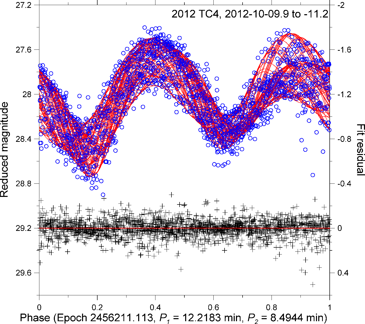
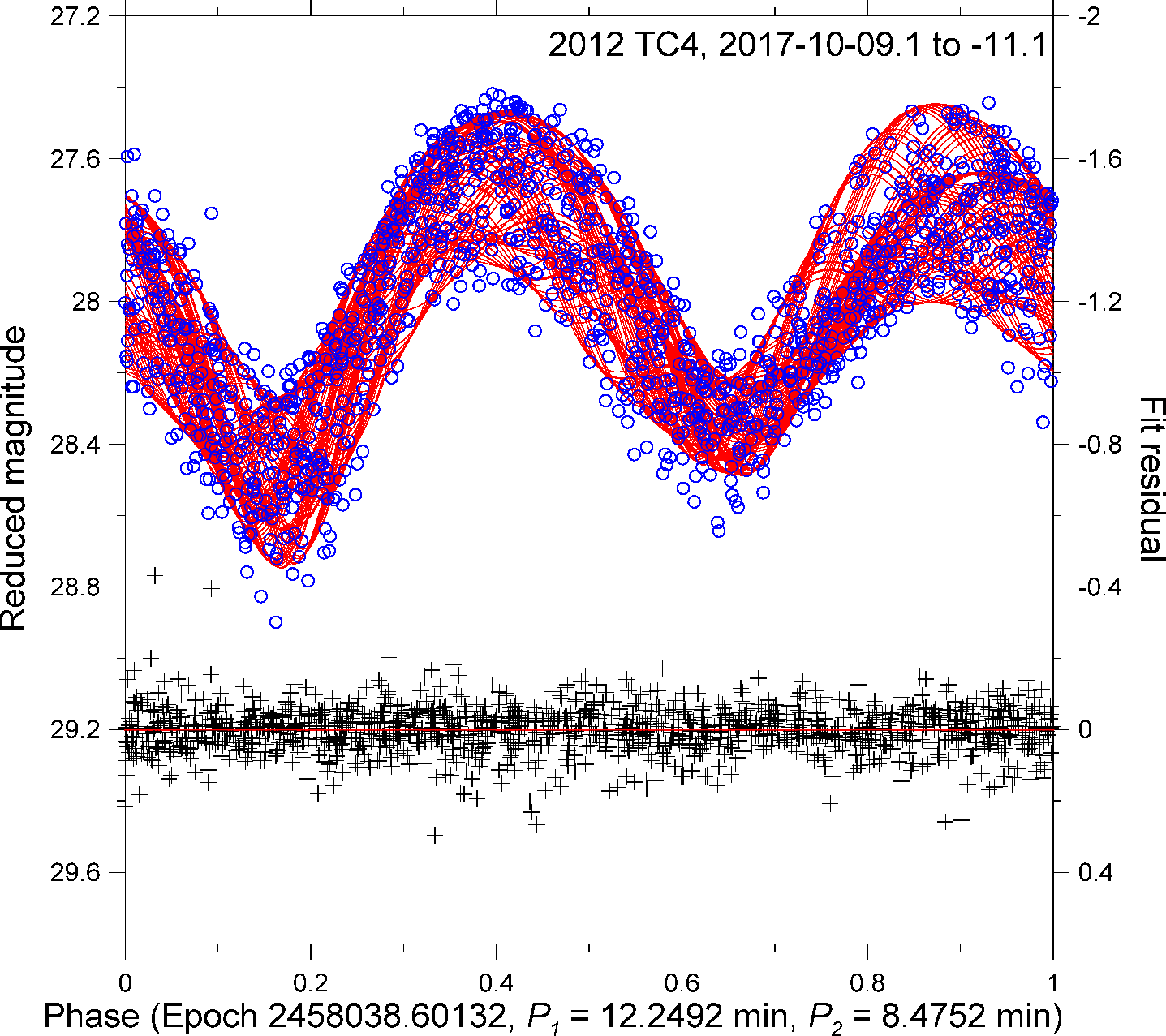
Figure 1: The blue open circles are the photometric data of 2012 TC4 taken from 2012-10-09.9 to 2012-10-11.2 (left) and from 2017-10-09.1 to 2017-10-11.1 (right) reduced to the unit geo- and heliocentric distances and to a consistent solar phase (see text for details), folded with the respective main periods $P_{1}$. The red curve is the best-fit 4th order Fourier series with the two periods. The black plusses are the post-fit residuals (see the right ordinates).

Table 1: Observation details (new data denoted by name of a coauthor)

Telescope	Date (UT)	Filter	Ref.
– 2012 –
OAVdA 0.81-m (Italy)	2012 10 09.9	C	Carbognani (2014)
Pistoiese 0.6-m (Italy)	2012 10 09.9	R	Bacci
Pistoiese 0.6-m (Italy)	2012 10 10.0	R	Bacci
MRO 2.4-m (USA)	2012 10 10.2	V	Ryan & Ryan (2017)
Wise observatory 0.72-m (Israel)	2012 10 10.8	V	Polishook (2013)
OAVdA 0.81-m (Italy)	2012 10 10.8	C	Carbognani (2014)
PROMPT1 0.41-m (Chile)	2012 10 11.1	Lum	Pollock
MRO 2.4-m (USA)	2012 10 11.1	V	Ryan & Ryan (2017)
PDO 0.35-m (USA)a	2012 10 11.2	V	Warner (2013)
– 2017 –
Kitt Peak Mayall 4-m (USA)	2017 09 13.2	R	Reddy et al. (2019)
Kitt Peak Mayall 4-m (USA)	2017 09 14.1	R	Reddy et al. (2019)
Palomar Hale 5-m (USA)	2017 09 17.4	SR	Reddy et al. (2019)
Palomar Hale 5-m (USA)	2017 09 20.2	SR	Warner (2018)
SOAR 4.1-m (Chile)	2017 10 06.2	SR	Reddy et al. (2019)
PDO 0.35-m (USA)	2017 10 09.2	V	Warner (2018)
MRO 2.4-m (USA)	2017 10 09.2	V	Reddy et al. (2019)
Kiso 1.05-m (Japan)	2017 10 09.5	SG	Urakawa et al. (2019)
Wise observatory 0.72-m (Israel)	2017 10 09.8	V	Reddy et al. (2019)
LCO-C 1-m (Chile)	2017 10 10.1	SR, SI	Reddy et al. (2019)
LCO-A 1-m (Chile)	2017 10 10.1	SR	Reddy et al. (2019)
PDO 0.35-m (USA)	2017 10 10.2	V	Warner (2018)
Nayoro 0.4-m (Japan)	2017 10 10.4	V	Urakawa et al. (2019)
BSGC 1-m (Japan)	2017 10 10.6	SG, SR, SI, SZ	Urakawa et al. (2019)
Lulin 1-m (Taiwan)b	2017 10 10.6	BVRI (diff.)	Lin et al. (2019)
Kiso 1.05-m (Japan)	2017 10 10.5	SG	Urakawa et al. (2019)
Wise observatory 0.72-m (Israel)	2017 10 10.8	V	Reddy et al. (2019)
Pistoiese 0.6-m (Italy)	2017 10 10.9	R	Bacci
KMTNet 1.6-m (South Africa)	2017 10 10.9	V	Reddy et al. (2019)
Pistoiese 0.6-m (Italy)	2017 10 11.0	R	Bacci
USNA 0.51-m (USA)	2017 10 11.0	V	Reddy et al. (2019)
MRO 2.4-m (USA)	2017 10 11.1	R	Reddy et al. (2019)
PDO 0.35-m (USA)	2017 10 11.2	V	Warner (2018)
Kiso 1.05 m (Japan)c	2017 10 11.5	SG	Urakawa et al. (2019)
Lulin 1-m (Taiwan)b	2017 10 11.6	BVRI (diff.)	Lin et al. (2019)
Anan Science Center 1.13-m (Japan)c	2017 10 11.6	V	Urakawa et al. (2019)
Wise Observatory 0.72-m (Israel)	2017 10 11.8	V	Reddy et al. (2019)
AIRA 0.38-m (Romania)	2017 10 11.8	V	Sonka et al. (2017)
Wildberg Observatory 0.35-m (Germany)d	2017 10 11.8		Apitzsch
KMTNet 1.6-m (South Africa)	2017 10 11.9	V	Reddy et al. (2019)
MRO 2.4-m (USA)	2017 10 12.1	R	Reddy et al. (2019)

3 Physical Model

3.1 Model from 2017 data

The light curve data set from 2017 is much richer than that from 2012, so we started with the inversion of 2017 data. We investigated possible frequency combinations based on the fact that the main frequencies $f_{1}$ and $f_{2}$ of a tumbling asteroid light curve are usually found at 2$f_{\phi}$ and 2($f_{\phi}\pm f_{\psi}$) or low harmonics and combination, where $f_{\phi}$ is the precession and $f_{\psi}$ the rotation frequency, respectively, and the plus sign is for a long-axis mode (LAM) and the minus sign for a short-axis mode (SAM) (Kaasalainen, 2001). Using the values $f_{1}=4.898\,\text{hr}^{-1}$ and $f_{2}=7.079\,\text{hr}^{-1}$ from the previous section, we found eight possible frequency combinations: $f_{1}=f_{\phi}$, $f_{2}=2(f_{\phi}-f_{\psi})$ (SAM1); $f_{1}=2(f_{\phi}-f_{\psi}),f_{2}=2f_{\phi}$ (SAM2); $f_{1}=2(f_{\phi}-f_{\psi}),f_{2}=f_{\phi}$ (SAM3); $f_{1}=f_{\phi}-f_{\psi},f_{2}=f_{\phi}$ (SAM4); $f_{1}=2f_{\phi},f_{2}=2(f_{\phi}+f_{\psi})$ (LAM1); $f_{1}=2f_{\phi},f_{2}=f_{\phi}+f_{\psi}$ (LAM2); $f_{1}=f_{\phi},f_{2}=(f_{\phi}+f_{\psi})$ (LAM3); $f_{1}=f_{\phi}+f_{\psi},f_{2}=f_{\phi}$ (LAM4). Then we conducted the shape and spin optimization for these combinations with the same way as in Lee et al. (2020). It was found that only the SAM4 solution provided an acceptable fit to the data and was physically self consistent.

We used 34 light curves from October 2017. Four light curves from September 2017 were very noisy and did not further constrain the model, so we did not include them in our analysis. We inverted the light curves with the method and code developed by Kaasalainen (2001) combined with Hapke’s light-scattering model (Hapke, 1993). According to Reddy et al. (2019), colors of TC4 are consistent with C or X complex and also its spectrum is X type, with Xc type being the best match. The X complex contains low and high albedo objects but the E type seems most likely because the high circular polarization ratio suggests that TC4 is optically bright (Reddy et al., 2019). This is in agreement with Urakawa et al. (2019) who also report X type colors. As a result we used Hapke’s model with parameters derived for an E type asteroid (2867) Šteins (Spjuth et al., 2012): $\varpi=0.57$, $g=-0.30$, $h=0.062$, $B_{0}=0.6$, and $\bar{\theta}=28^{\circ}$. Because our data did not cover low solar phase angles, $h$ and $B_{0}$ parameters for opposition surge and also roughness $\bar{\theta}$ were fixed. We optimized $\varpi$ and $g$ parameters and they converged to values $\varpi=0.69$, $g=-0.20$, which gave geometric albedo of 0.34. An alternative solution with fixed values $\varpi=0.57$, $g=-0.30$ provided only marginally worse fit and the kinematic parameters were not affected. In general, solution of our inverse problem was not sensitive to Hapke’s parameters likewise in previous studies (e.g., Scheirich et al., 2010; Pravec et al., 2014; Lee et al., 2020).

The rotation and precession periods had the following values: $P_{\psi}=27.5070\pm 0.002$ min and $P_{\phi}=8.47512\pm 0.0002$ min, respectively. The $1\sigma$ uncertainties were estimated from the increase of $\chi^{2}$ when varying the solved-for parameters – given the number of measurements about 8600, $3\sigma$ uncertainty interval corresponds to about 5% increase in $\chi^{2}$ (e.g., Vokrouhlický et al., 2017). Direction of the angular momentum vector in ecliptic coordinates was $\lambda=92^{\circ}$, $\beta=-89.6^{\circ}$, practically oriented toward the south ecliptic pole. Normalized moments of inertia were $I_{1}=0.41$, $I_{2}=0.81$, but the model was not too sensitive to their particular values. The inertia moments computed from the 3D shape (assuming constant density) were $I_{1}=0.435$, $I_{2}=0.831$, indicating consistency with the kinematic parameters above.

The dark facet, which is always introduced into a convex shape model to regularize the solution (Kaasalainen & Torppa, 2001), represented about a few percent of the total surface area and forcing it to smaller values led to a worse fit. This might mean that there is some albedo variegation on the surface of TC4 or that its real shape is highly nonconvex and a convex-shape approximation represent its limits.

3.2 Model from 2012 data

For this model, we used 14 light curves from 2012. The rotation and precession periods were now $P_{\psi}=27.873\pm 0.005$ min and $P_{\phi}=8.4945\pm 0.0003$ min, respectively. The $1\sigma$ uncertainties were estimated in the same way as for the 2017 model, namely from the increase of $\chi^{2}$. The direction of the angular momentum vector was $\lambda=89^{\circ}$, $\beta=-90^{\circ}$, moments of inertia $I_{1}=0.43$, $I_{2}=0.80$. The 3D shape model was similar to that reconstructed from 2017 data and also the direction of the angular momentum vector was practically the same.

In spite of consistency in all other solved-for parameters, we thus observed that the periods $P_{\phi}$ and $P_{\psi}$ for the two apparitions were significantly different. Attempts to use the 2017 values to fit the 2012 data, or vice versa, led to a dramatically worse fit. We scanned period parameter space around the best-fit values and plotted the relative $\chi^{2}$ values – see Fig. 2. The minima in $\chi^{2}$ for 2012 and 2017 periods are clearly separated.

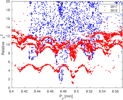
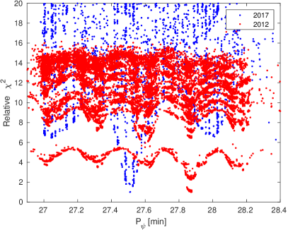
Figure 2: Period scan for data from 2017 (October only) and 2012. Each point represents one trial model that converged to given $P_{\phi}$, $P_{\psi}$, and $\chi^{2}$ values. Minima for 2012 and 2017 data are clearly separated. Relative $\chi^{2}$ was normalized to have the minimum value of 1.

3.3 Model from 2012 and 2017 data

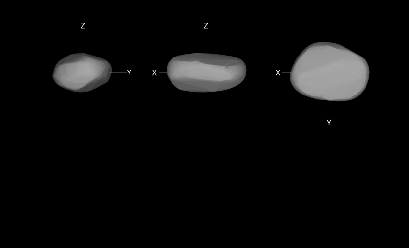
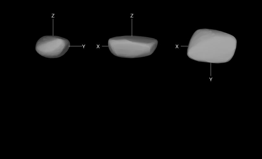
Figure 3: Shape models reconstructed independently from 2012 (top) and 2017 (bottom) light curves. The 2017 model is also almost identical to that reconstructed from joint inversion of 2012 and 2017 data.

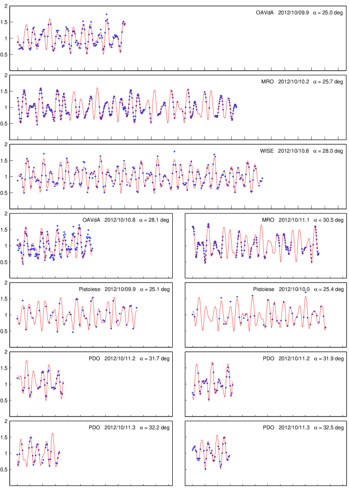
Figure 11: Light curve fits for data in 2012. The photometric light curve data shown in this figure is available as ”Data behind the Figure.”

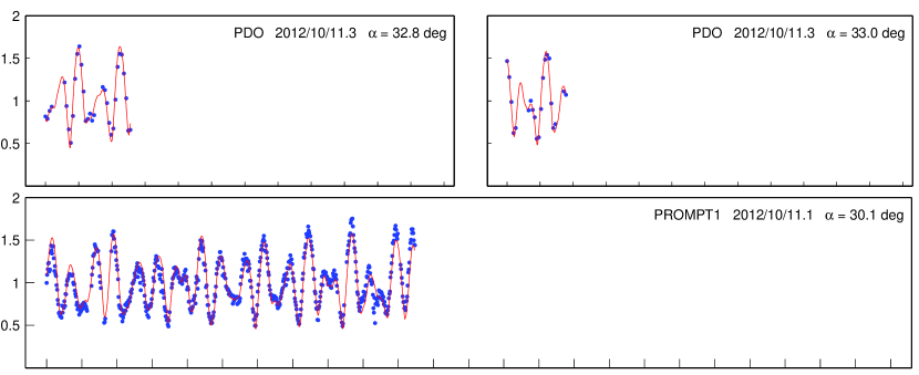
Figure 12: Light curve fits for data in 2012. The photometric light curve data shown in this figure is available as ”Data behind the Figure.”

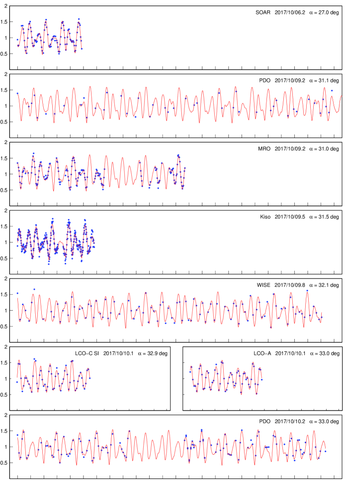
Figure 13: Light curve fits for data in 2017. The photometric light curve data shown in this figure is available as ”Data behind the Figure.”

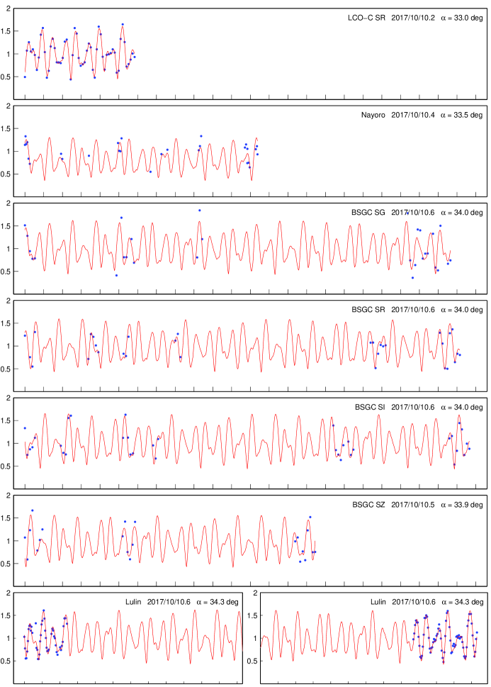
Figure 14: Light curve fits for data in 2017. The photometric light curve data shown in this figure is available as ”Data behind the Figure.”

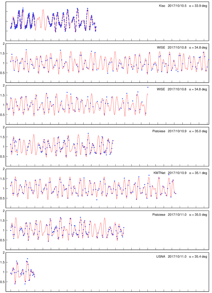
Figure 15: Light curve fits for data in 2017. The photometric light curve data shown in this figure is available as ”Data behind the Figure.”

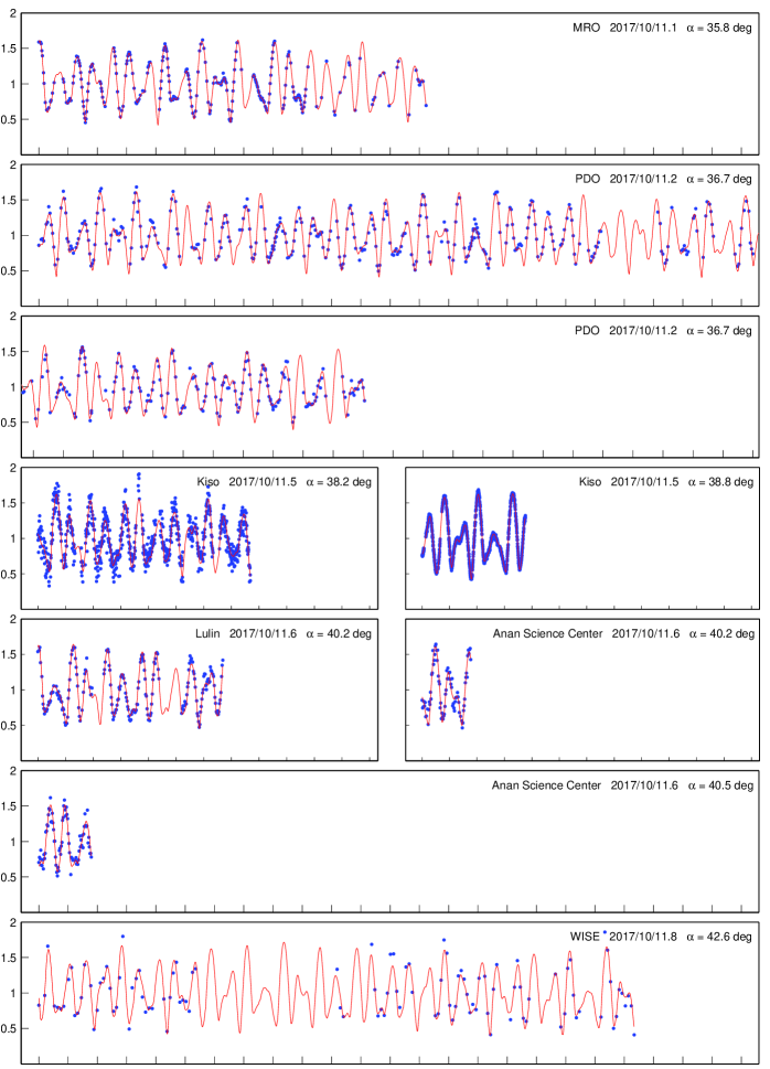
Figure 16: Light curve fits for data in 2017. The photometric light curve data shown in this figure is available as ”Data behind the Figure.”

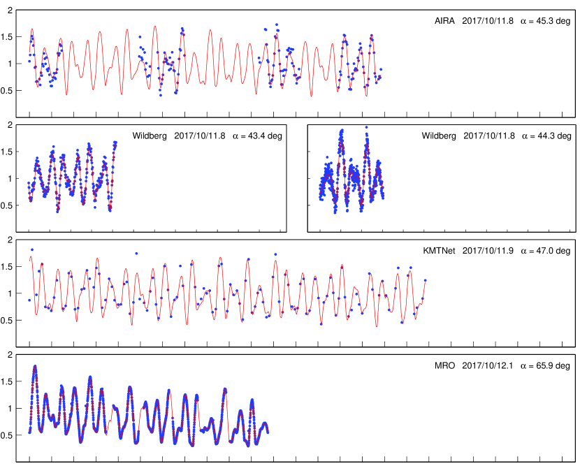
Figure 17: Light curve fits for data in 2017. The photometric light curve data shown in this figure is available as ”Data behind the Figure.”

The 3D models reconstructed from the two apparitions independently have similar global shapes but their details are different (Fig. 3). If we take the shape reconstructed from the 2017 data and use it to fit the 2012 data, it gives a satisfactory fit to light curves. However, a better way how to use all data together is not to treat them separately but to instead invert both apparitions together with a common shape model that would differ only in kinematic parameters. Therefore, we modified the original inversion code of Kaasalainen (2001) to enable including two independent light curve sets. We assumed that the only parameters that were different for the two apparitions were the rotation and precession periods $P_{\psi}$, $P_{\phi}$ and initial Euler angles $\phi_{0}$, $\psi_{0}$. Parameters describing the shape and the direction of the angular momentum vector were the same. So the full set of kinematic parameters for a two-apparition model was: $(\lambda,\beta,\phi_{0}^{(1)},\phi_{0}^{(2)},\psi_{0}^{(1)},\psi_{0}^{(2)},P_{\psi}^{(1)},P_{\psi}^{(2)},P_{\phi}^{(1)},P_{\phi}^{(2)},I_{1},I_{2})$, where the superscript $(1)$ is for 2012 apparition and $(2)$ is for 2017 apparition. The two light curve data sets were independent in the sense that the integration of kinematic equations (eq. A.3 in Kaasalainen, 2001) was done separately for 2012 and 2017 data, the two epochs were not directly connected. The final model shape is almost identical to that reconstructed from only 2017 data shown in Fig. 3. The fit of the final model to individual light curves is shown in Figs. 11–17. Rotation and precession periods converged to practically the same values as with the independent treatment of each of two apparitions. The best-fit parameters for the 2012 and 2017 apparitions are listed in Table 2. The physical models of 2012 TC4 from 2012 and 2017 and the light curve data set used to reconstruct these models are available from the DAMIT database (Ďurech et al., 2010).

Table 2: Parameters of the model in Fig. 3 reconstructed from 2012 and 2017 light curves. The reported errors correspond to standard deviations of parameters computed from bootstrap models. Parameters without errors were fixed (Hapke’s parameters) or did not change ($I_{1}$ and $I_{2}$). Formally small uncertainty of $\psi_{0}$ means that this initial orientation angle is correlated with the shape and does not change significantly with different bootstrap data sets. Parameter $\lambda$ is practically unconstrained because the angular momentum direction is very close to $\beta=-90^{\circ}$. Values $\delta L/L$ and $\delta E/E$ are relative changes of angular momentum $L$ and energy $E$ between 2012 and 2017, i.e., $\delta L/L=(L_{2017}-L_{2012})/L_{2017}$ and $\delta E/E=(E_{2017}-E_{2012})/E_{2017}$.

	2012	2017
$P_{\psi}$ [min]	$27.8720\pm 0.0007$	$27.5070\pm 0.0002\$
$P_{\phi}$ [min]	$\ 8.4944\pm 0.0005$	$\ 8.47511\pm 0.00008$
$\phi_{0}$ [deg]	$322\pm 8$	$74\pm 9$
$\psi_{0}$ [deg]	$198\pm 0.02$	$180\pm 0.2$
JD0	2456210.00	2458032.69
$\lambda$ [deg]	$103\pm 78$
$\beta$ [deg]	$-88.5\pm 0.7$
$I_{1}$	0.42
$I_{2}$	0.81
$w$	0.67
$g$	$-0.20$
$h$	0.062
$B_{0}$	0.6
$\bar{\theta}$ [deg]	28
$\delta L/L$	$0.00078\pm 0.00006$
$\delta E/E$	$-0.0035\pm 0.0001$

3.4 Bootstrap

To estimate uncertainties of physical periods, and to further robustly demonstrate that their change between 2012 and 2017 is significant, we created bootstrapped data samples and repeated the light curve inversion for them. From both 2012 and 2017 data sets, we created 1000 bootstrap samples by randomly selecting the same number of light curves from the original data set. For October 2017 bootstrap, 279 final shape models had clearly wrong inertia tensor that was not consistent with the kinematic $I_{1},I_{2}$ parameters, so we removed them from the analysis. For all remaining bootstrap models, we plot histograms of $P_{\phi}$ and $P_{\psi}$ distribution in Fig. 4. The standard deviations of the precession period $P_{\phi}$ are $0.0005\,$min and $0.00009\,$min for 2012 and 2017 data, respectively, which are similar to uncertainty values derived in Sects. 3.1 and 3.2. For the rotation period $P_{\psi}$, these standard deviations are $0.0008$ and $0.0002$ min, which is significantly smaller than our $\chi^{2}$-based estimate. Nevertheless, the difference between periods determined from 2012 and 2017 apparitions is much larger than their uncertainty intervals and we are not aware of any random or model errors that could cause such difference. Our conclusion is that the spin state of TC4 has changed from 2012 to 2017, rotation and precession periods have decreased. In what follows, we try to interpret this change using a theoretical model of TC4 spin evolution with the relevant torques.

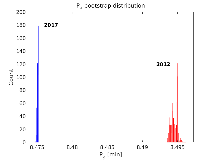
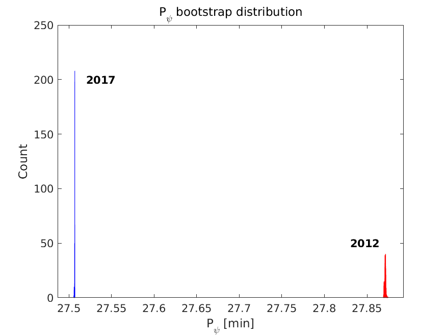
Figure 4: Distribution of periods $P_{\phi}$ (left) and $P_{\psi}$ (right) for bootstrapped light curves.

4 Theory

4.1 Orbital dynamics

The unique observational opportunities of 2012 TC4 are directly related to its exceptional orbit. The asteroid had a deep encounter with the Earth on October 12, 2012, during which the closest distance to the geocenter was approximately $95,000$ km (Fig. 5). However, the more unusual circumstance was that the 2012 close encounter resulted in a change of the 2012 TC4’s orbital semimajor axis which placed it nearly exactly to the 5:3 resonance with the Earth heliocentric motion. As a result, in five years after the first close encounter, i.e. on October 12, 2017, the relative configuration of the asteroid and the Earth nearly exactly repeated, placing it again in a deep encounter configuration. This time the closest approach to the geocenter had even closer distance of $50,200$ km. Astrometric observations during the two close approaches, including Arecibo and Green Bank radar data taken in 2017, allowed a very accurate orbital solution over the five year period of time in between 2012 and 2017. In the context of this paper, we note that it also provided an interesting information about nongravitational effects needed to be empirically included in orbit determination. Adopting methodology from cometary motion (e.g., Marsden et al. (1973) and Farnocchia et al. (2013) or Mommert et al. (2014) for the asteroidal context), we note the following values of radial $A_{1}$ and transverse $A_{2}$ accelerations: (i) $A_{1}=(2.17\pm 0.80)\times 10^{-11}$ au d^-2, or $(4.35\pm 1.60)\times 10^{-10}$ m s^-2, and (ii) $A_{2}=-(2.73\pm 0.65)\times 10^{-13}$ au d^-2 (both assume $\propto r^{-2}$ heliocentric decrease; see JPL/Horizons web page https://ssd.jpl.nasa.gov/sbdb.cgi). At a first sight, these values appear very reasonable (compare, e.g., with a $A_{1}$ and $A_{2}$ fits for a $\simeq 4$ m body 2009 BD, Mommert et al., 2014; Vokrouhlický et al., 2015a).

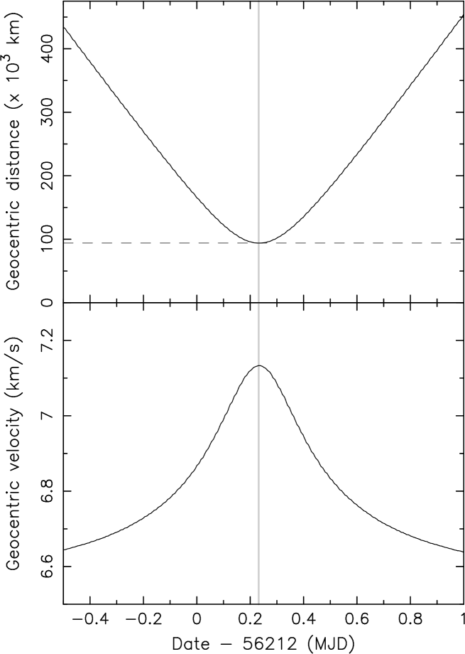
Figure 5: Geocentric distance (top) and relative velocity (bottom) of 2012 TC4 during its close encounter with Earth on October 12, 2012 (nominal minimum configuration at MJD56212.229, gray vertical line); the abscissa shows time in days with respect to MJD56212. The dashed horizontal line at the top panel shows the minimum distance of $\simeq 95,000$ km. The asymptotic value of the relative velocity with respect to the Earth, $\simeq 6.5$ km/s, increases to more than $7.1$ km/s by the Earth gravity.

If we were to interpret both components as a result of radiation forces, we may further obtain useful information about the body. The radial component would represent the direct solar radiation pressure. In a simple model, where we assume a spherical body of size $D$ and bulk density $\rho$, we have $A_{1}\simeq 3C_{\rm R}F_{0}/(2\rho Dc)$, with $C_{\rm R}$ the radiation pressure coefficient (dependent on sunlight scattering properties on the surface), $F_{0}\simeq 1367$ W m^-2 the solar constant and $c$ the light velocity. Adopting $C_{\rm R}\simeq 1.2$ and $D\simeq 10$ m, we obtain a very reasonable bulk density $\rho\simeq(1.9\pm 0.7)$ g cm^-3. The transverse component of nongravitational orbital effects makes sense when interpreted as the Yarkovsky effect (e.g., Vokrouhlický et al., 2015a). Note that the above mentioned value of $A_{2}$ translates to a secular change of the semimajor axis $da/dt=-(110\pm 26)\times 10^{-4}$ au My^-1 (see, e.g., Farnocchia et al., 2013). Given the near extreme obliquity of the rotational angular momentum, we may safely restrict to the diurnal component of the Yarkovsky effect. The negative value of $A_{2}$, or $da/dt$, corresponds well to the retrograde sense of 2012 TC4 rotation (implied by the direction of the rotational angular momentum vector, Sec. 3). Next, borrowing the simple model for a spherical body from Vokrouhlický (1998), and fixing the size $D=10$ m, the inferred bulk density $\rho\simeq 1.9$ g cm^-3 and the surface thermal conductivity $K=0.05$ W m^-1 K^-1, we estimate that the corresponding surface thermal inertia is $\Gamma\simeq 490^{+270}_{-250}$ in SI units (though, we note there is also a lower-inertia solution possible like in Mommert et al., 2014). This is a very adequate value too (e.g., Delbó et al., 2015). Obviously, due to many frozen parameters in the model (and its simplicity), the realistic uncertainty in $\Gamma$ would be larger. However, it is not our intention to fully solve this problem. We satisfy ourselves with observation that the needed empirical nongravitational accelerations in the orbital fit may be very satisfactorily interpreted as radiation-related effects. In the next sections, we show that also the change in the rotation state in between 2012 and 2017 observation epochs may be very well explained by the radiation torque known as the Yarkovsky-O’Keefe-Radzievskii-Paddack effect (e.g., Vokrouhlický et al., 2015a).

4.2 Rotational dynamics

Our methods and mathematical approach used to describe evolution of the rotation state of 2012 TC4 are presented in the Appendix A, therefore here we provide just a general outline. We numerically integrated Euler equations (A2) and (A4) describing spin state evolution of 2012 TC4 in between the observation runs in 2012 and 2017. The kinematical part, describing transformation between the inertial frame and the body-frame defined by principal axes of the tensor of inertia, was parametrized by the Rodrigues-Hamilton parameters $\mbox{\boldmath$\lambda$}=(\lambda_{0},\lambda_{1},\lambda_{2},\lambda_{3})$ (see, e.g., Whittaker, 1917). This choice helps to remove problems related to coordinate singularity given by zero value of the nutation angle. The dynamical part is represented by evolution of the angular velocity $\omega$ in the body-frame. Note that in most cases of asteroid lightcurve interpretation, a simplified model of a free-top would be sufficient (used also in Sec. 3 to fit the 2012 and 2017 data separately). However, the evidence of change of the rotation state of 2012 TC4 in between the 2012 and 2017 epochs, discussed above, requires appropriate torques to be included in the model. We addressed two effects:

• gravitational torques due to the Sun and the Earth, and

• radiation torques due to the sunlight scattered by the surface and thermally re-radiated (the YORP effect; e.g., Bottke et al., 2006; Vokrouhlický et al., 2015a).

The tidal gravitational fields of the Sun and the Earth were represented in the body-frame using the quadrupole approximation (A7) (e.g., Fitzpatrick, 1970; Takahashi et al., 2013). The nature of the perturbation is different for the Sun and the Earth. In the solar case, the gravitational torque results in a small tilt by less than $1$ arcminute describing a small segment on the precession cone. The effect of the Earth-induced gravitational torques manifests as an impulsive effect only during close encounters. Our main goal was to verify that, due to fast rotation of 2012 TC4, the effect averages out and cannot contribute to the observed change in rotational frequencies. Indeed, Fig. 6 shows change of the osculating rotational (intrinsic) angular momentum and energy during the 2012 close encounter with the Earth (only about six times larger effects are observed during the closer encounter in 2017, but this is not relevant for our analysis anyway, because observations preceded this approach). The initial data of the simulation were taken from the observations fit in 2012, namely before the encounter. Recall that the characteristic timescale of the encounter is about half a day (determined, for instance, as a width of characteristic Earth relative velocity increase at the bottom panel of Fig. 5 at $\simeq 6.8$ km s^-1 level, half value between the asymptotic and peak velocities). In comparison, the characteristic rotational periods $P_{\psi}$ and $P_{\phi}$ are of the order of minutes, i.e. much shorter. As a result, the effect of the Earth gravitational torque efficiently averages out during each of the rotation cycles (a significant effect may be expected only for very slowly rotating bodies and sufficiently deep encounters, such as seen for 4179 Toutatis during its 2004 close encounter with the Earth; e.g., Takahashi et al., 2013). Therefore, we may conclude that the gravitational torques cannot explain the observed change in the rotation state of 2012 TC4 in between the 2012 and 2017 epochs. Still, we keep them in our model for the sake of completeness.

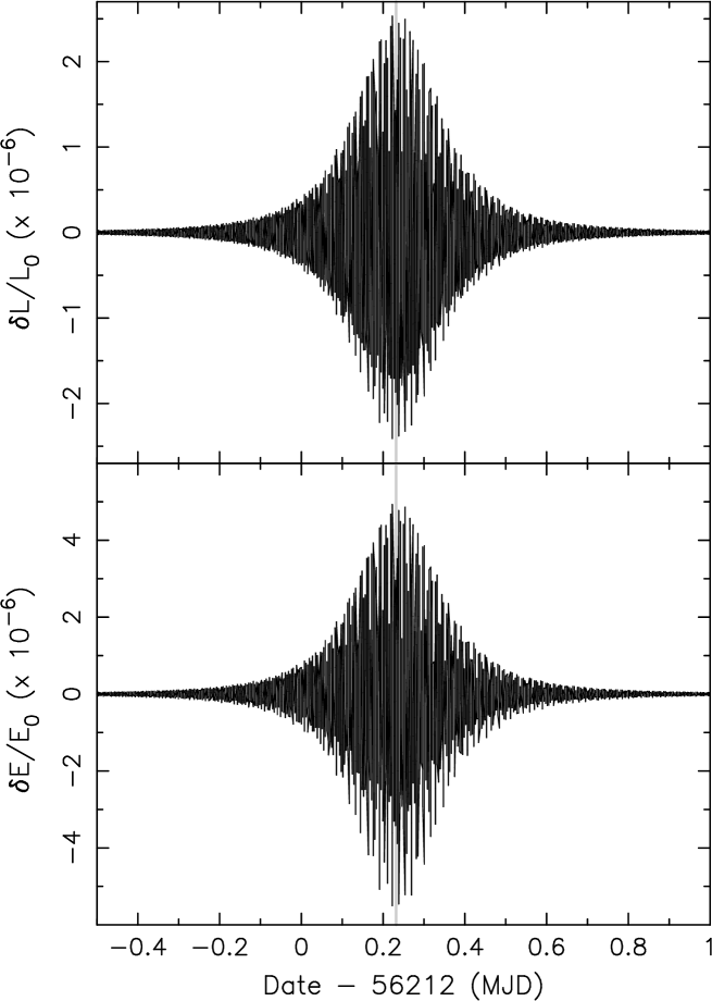
Figure 6: The effect of the Earth gravitational torque in quadrupole approximation on rotation state parameters of 2012 TC4 during its close encounter on October 12, 2012 (gray line denotes the nominal minimum distance configuration). The abscissa shows time in days with respect to MJD56212 (as in Fig. 5). The upper panel shows a fractional change of the rotational angular momentum $\delta L=L-L_{0}$, normalized by the initial value $L_{0}$, the bottom panel panel shows a fractional change of the rotational energy $\delta E=E-E_{0}$, normalized by the initial value $E_{0}$ (note that both ordinate scales are in $10^{-6}$). The resulting change of both parameters after the encounter is $\leq 5\times 10^{-9}$.

Figure 7: The effect of the radiation (YORP) torque on rotation state parameters of 2012 TC4 in the time interval between the two recent close encounters with the Earth (i.e., October 12, 2012 and October 12, 2017). Nominal model is used here to obtain a first insight of the expected order of magnitude of the perturbation. The abscissa shows time in years. The upper panel shows a fractional change of the rotational angular momentum $\delta L=L-L_{0}$, normalized by the initial value $L_{0}$, the bottom panel panel shows a fractional change of the rotational energy $\delta E=E-E_{0}$, normalized by the initial value $E_{0}$ (note that both ordinate scales are in $10^{-3}$). Both reference values taken at MJD58032.19, mean epoch of 2017 observations, and the asteroid’s rotation state was propagated backward in time to October 2012.

The radiation torques are of a quite different importance. It is well-known that the YORP effect is able to secularly change rotational frequency and tilt the rotational angular momentum in space. While mostly studied in the limit of a rotation about the shortest axis of the inertial tensor, generalizations to the tumbling situation were also developed. Both numerical (Vokrouhlický et al., 2007) and analytical (Cicalò & Scheeres, 2010; Breiter et al., 2011) studies confirmed that YORP effect is able to change rotational angular momentum, its orientation in both the inertial space and body-frame in an appreciable manner. As usual, the effect is more important on small bodies. Here we included the simple, zero-inertia limit developed in Rubincam (2000) and Vokrouhlický & Čapek (2002), see Eq. (A8). A first look into importance of the radiation torques may be obtained by taking nominal solution of the rotation state from the 2017 observations, including the appropriate shape model, and propagate it backwards in time to early October 2012 (epoch of the first set of observations). We use the more accurate 2017 model as reference rather than the one constructed from poorer 2012 observations. The length-scale of the model was adjusted to correspond to an equivalent sphere of diameter $D=10$ m and density was $\rho=1.4$ g cm^-3. We verified that results have the expected invariance to rescaling of both $\rho$ and $D$ such that $\rho\,D^{2}=$ const. Our nominal choice of the $1.4$ g cm^-3 bulk density, albeit conflicting with the suggested E-type specral classification of TC4, is therefore linked to the assumed equivalent size of $10$ m, but it might be redefined according to the rescaling principle. This combination of parameters provides a very nice match of the $P_{\phi}$ period change due to our YORP model (see Sec. 4.3).

Figure 7 provides information about secular change in rotational angular momentum $L$ (top) and energy $E$ (bottom) in that simulation. Here we see a long-term change in both quantities. The wavy pattern is due to eccentricity of the 2012 TC4 orbit and a stronger YORP torque at perihelion. The accumulated fractional change in both $L$ and $E$ is few times $10^{-3}$. This is promising, because the observed change in these quantities in of the same order of magnitude (see Table 2), and makes us believe that the change in the directly observable $P_{\psi}$ and $P_{\phi}$ periods will also be as needed. Nevertheless, we also note a difference. The simulation results shown in Fig. 7 indicate both angular momentum and energy increased from 2012 to 2017. Such a behaviour is perhaps expected at the first place (for instance, in the case of a body in a principal-rotation state, YORP would necessarily affect both $E$ and $L$ in the same way). However, rotation state solutions from observations in 2012 and 2017 tell us something else (see Table 2): the rotational angular momentum $L$ increased in between 2012 and 2017, while the energy $E$ decreased. Before commenting more on this difference, we first provide more detailed analysis of the radiation torque effects for 2012 TC4 in our modeling, this time using the whole suite of acceptable initial data and shape models (all compatible with the observations; Sec. 3.4). This will allow a statistical assessment of the predicted values.

4.3 Results

An ideal procedure of proving that the observed changes in tumbling-state periods $P_{\phi}$ and $P_{\psi}$ are due to the radiation (YORP) torques would require a highly-reliable theoretical model (numerical propagation of 2012 TC4’s rotation state with appropriate torques included) employed to fit all available observations (in our case data from October 2012 and 2017). Obviously, the only “comfort” of this analysis would be to possibly adjust some free (unknown) parameters. Unfortunately, such a plan is presently too ambitious, and thus we resort to a simpler way.

Recall the much easier situation when the YORP effect has been searched (and detected) for asteroids rotating in the lowest-energy mode, namely about the shortest principal axis of the inertia tensor. In this case, YORP results in a secular change of the unique rotation period $P$ (as in $P_{\phi}$ and $P_{\psi}$, when the body tumbles). The measurements are rarely precise enough, and the effect strong enough, to directly reveal the change in the period $P$ (see, though, an exception for 54509 YORP, Lowry et al., 2007). More often, one uses the fact that the linear-in-time change in $P$ produces a quadratic-in-time effect in the rotation-phase. Linking properly the asteroid rotation phase over many observation sessions with an empirical quadratic term helps to characterize changes of $P$ which are individually too small to be determined from one-apparition observations (see, e.g., Vokrouhlický et al., 2015a). This approach adopts an empirical magnitude of the quadratic term in the rotation phase and simply solves it as a free parameter (not combining it with a theoretical model at that stage). Interpretation in terms of the YORP effect is done only aposteriori, when the fitted amplitude of the phase-quadratic term is compared with a prediction from the YORP model. And even then, the comparison is often not simple, because the model prediction for YORP is known to depend on unresolved small-scale irregularities of the body shape. At several occasions one had to satisfy with a factor of few difference accounting for the model inaccuracy.

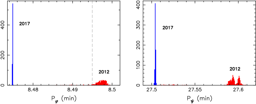
Figure 8: Distribution of periods $P_{\phi}$ (left) and $P_{\psi}$ (right) for 687 models of 2012 TC4 from our numerical simulation containing both gravitational and radiation (YORP) torques. The individual models sample possible initial orientation of the angular momentum vector $\mathbf{L}$ in the inertial space, orientation of the body-frame in the inertial space and slight shape variants of the body. All models were constructed using the October 2017 observations and therefore they are referred to the common epoch MJD58032.19. Blue histograms are computed from these initial data and they are identical to those in Fig. 4. The red histograms correspond to the rotation state of 2012 TC4 at MJD56209.88, nominal epoch of the October 2012 observations (the mean $P_{\phi}$ value from the observations is shown with the vertical dashed line). Unlike in Fig. 4, the 2012 data here were computed from the spin state vectors obtained from our numerical propagation of the 2012 TC4 rotation starting in October 2017.

Things are quite more complex when the body tumbles. First of all, it is not clear how to set the empirical approach from above and apply it in this situation. In the same time, direct modeling approach is probably even less accurate than in the case of rotation about the principal axis of the inertia tensor. Not only the worry about the role of unresolved small-scale irregularities remains, but the present YORP model is restricted to the zero thermal conductivity limit (see, e.g., Vokrouhlický et al. (2007) for numerical approach, and Cicalò & Scheeres (2010); Breiter et al. (2011) for analytical studies). Yarkovsky acceleration for tumblers was evaluated with thermal models (e.g., Vokrouhlický et al., 2005, 2015b), but in these cases $P_{\phi}$ and $P_{\psi}$ were slightly tweaked to make them resonant (an approach we cannot afford here). In this situation, we adopted the following simple procedure.

4.3.1 Model based on 2017 data

We start with a set of models based uniquely on the most reliable and accurate observations from the 2017 apparition. In particular, we constructed 687 variants of the 2012 TC4 physical model (Sec. 3.1). They are all very similar, because they sample tight parameter variations all resulting in acceptable fits of the data. These represent (i) slightly modified initial rotation parameters (Euler angles and their derivatives, as well as inertial space direction of the rotational angular momentum vector), and (ii) slight shape variants of the body. The initial epoch MJD58032.19 was common to all variant models. Using these initial data and shape models, we propagated all 687 clone realizations of 2012 TC4 backward in time to the epoch MJD56209.88, characteristic of the October 2012 observations. We used our numerical approach described above with both gravitational and radiation (YORP) torques included. For the latter, we assumed an effective size $D=10$ m (corresponding to a sphere of the same volume of the models) and bulk density $\rho=1.4$ g cm^-3. The above-mentioned rescaling rule, namely invariance to $\rho\,D^{2}$, may allow us to transform our results to other combinations of $D$ and $\rho$ values.

The evolutionary tracks of angular momentum $L$ and energy $E$ secular changes due to the YORP torques mostly resemble those from Fig. 7. For some model variants, which were more different from the nominal one, the slope of the overall secular change in $L$ and/or $E$ was shallower or steeper. At the initial and final epochs of our simulations we determined $P_{\phi}$ and $P_{\psi}$ periods from a short numerical simulation of a free-top model. We also verified that the $P_{\psi}$ values correspond exactly to those provided by the analytical formula (A5). Figure 8 shows our results. The blue histograms are for the initial data, i.e., the October 2017 rotation state. Because the observations were numerous and of a good quality, the model variants differ only slightly and the $P_{\phi}$ and $P_{\psi}$ distributions are tight (they also match those from the Fig. 4). The red histograms in Fig. 8 were determined from the last epoch of our numerical runs and correspond to the predicted rotation state of 2012 TC4 in October 2012. We note both period appreciably changed, as already anticipated from preliminary simulation shown in Fig. 7. These $P_{\phi}$ and $P_{\psi}$ distributions are obviously less tight than the initial ones, reflecting different evolutionary tracks of the individual clone variants. Our prime interest is to compare the red distribution in Fig. 8 (from simulations) to the red distributions in Fig. 4 (from the 2012 observations, also highlighted withe dashed line for $P_{\phi}$ period). First, we note that the match of the $P_{\phi}$ periods is surprisingly good. The mean value $8.495$ min of the observations rather well corresponds to the mean value $8.497$ min of the simulated data, which have comfortably large dispersion of $0.003$ min to overlap with the observed data; in fact, the shift in $P_{\phi}$ is even larger than required. Interestingly, the comparison is not as good in the $P_{\psi}$ period. The model-predicted value $27.59\pm 0.02$ min (formal uncertainty) is short to explain the observations which provide on average $27.87$ min. Still, the model indicates a significant shift from the initial value $27.5070\pm 0.0002$ min. Nevertheless, to reach the value from the 2012 observations the shift would need to be about $3.7$ times larger. We do not know the reason for this difference, at all likelihood also related to the misbehaviour in the rotational energy evolution (see above). We suspect that the overly simple modeling of the YORP effect, such as the surface thermal inertia and/or the unresolved small-scale shape irregularities, play and important role here (note that a factor of $3$ between the observations and model-prediction was also seen in the cases when YORP was detected for asteroids rotating about the principal axis of the inertia tensor). The fact that some deeper aspects of the model are not characterized well, as witnessed by the opposite sign of the energy evolution, implies that our results cannot be easily reconciled with the observations by a simple rescaling of size $D$ and bulk density $\rho$. We have verified that the accumulated shifts in both $P_{\phi}$ and $P_{\psi}$ periods are proportional to $\rho\,D^{2}$. Thus, the $P_{\psi}$ mismatch could be explained by assuming the 2012 TC4’s size is $\simeq 5.2$ m, but this would produce factor $\simeq 3.7$ inconsistency in $P_{\phi}$ period (making the modeled value larger than observed). Instead, we believe that some missing details of the YORP modeling, which result in different effects on $P_{\phi}$ and $P_{\psi}$, are responsible for the difference.

4.3.2 Model based on a combination of 2012 and 2017 data

For sake of comparison, we also repeated our analysis using models based on a combination of the observations in 2012 and 2017 (Sec. 3.3). Obviously at each of these epochs we considered different parameters of the rotation state, but now we enforced the same shape model is used for both data-sets. This solution gives us an opportunity to consider two sets of initial conditions for our simulation, both in 2012 and 2017, and analyses predictions in the complementary epoch (integrating the rotation model once backward in time and once forward in time). Obviously, in all cases our model includes the gravitational and radiation torques, $D=10$ m effective size and $\rho=1.4$ g cm^-3 bulk density as before (needed for the evaluation of the radiation torques).

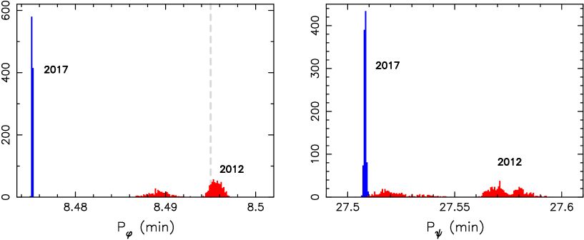
Figure 9: The same as in Fig. 8, but now for nearly a thousand variant shape models of 2012 TC4 constructed from a combination of the 2012 and 2017 data. Data at the initial epoch MJD58032.19 (October 2017) are in blue. They have been propagated using our dynamical model to MJD56209.88 (October 2012), and the endstates of these runs served to compute $P_{\phi}$ and $P_{\psi}$ shown by the red histograms.

We start with the case of the initial data in October 2017 and backward-in-time integration. This is directly comparable with results above, when only observations in 2017 were used. However, the models are slightly different in all their aspects (initial conditions and shape), because now the 2012 observations play the role in their construction. Results are shown in Fig. 9. While slightly different then in Fig. 8, the principal outcome is the same: (i) fairly satisfactory prediction for the $P_{\phi}$ period, while (ii) too small change in the $P_{\psi}$ period.

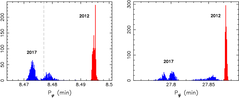
Figure 10: The same as in Fig. 9 (shape models constrained by both 2012 and 2017 observations), but now propagation was performed from MJD56209.5 epoch in 2012 (red) to MJD58032.19 in 2017 (blue). The 2012 data constrain the rotation state solution less accurately and thus result in a larger scatter of the predicted periods $P_{\phi}$ and $P_{\psi}$ in 2017. The vertical dashed line shows mean value of the $P_{\phi}$ period from the October 2017 observations.

We next consider the opposite case, namely initial condition in October 2012 and model propagation forward in time to October 2017. Results are shown in Fig. 10. Obviously, here the red histograms (from initial data in October 2012) are more constrained than the blue histograms (resulting from rotation state vectors propagated using our model to October 2017). The latter are more dispersed than the red histograms in Fig. 9, because the less numerous and accurate observations in 2012 constrain the models with lower accuracy. Nevertheless, the principal features of the solution are still present: (i) the $P_{\phi}$ period changed adequately for majority of cases, while (ii) the $P_{\psi}$ period changed too little.

4.3.3 In summary

So while we are not able to provide an exact proof that the change in $P_{\phi}$ and $P_{\psi}$ periods between the 2012 and 2017 apparitions of 2012 TC4 are due to the YORP effect, we consider the difference between the observations and model predictions can be accounted for the model inaccuracy.

5 Discussion

In the previous section, we demonstrated that the observed change of the rotation state of 2012 TC4 in between the two apparitions in 2012 and 2017 may be possibly explained as a result of the YORP effect. We also showed that the effect of the close encounter in October 12, 2012 on the rotation state was minimum, at least in a rigid-body approximation. However, since the YORP model –for the reasons explained– did not provide an exact match of the observations, and even left unresolved the issue of the observed energy change versus the model prediction, it is both useful and necessary to also briefly analyse possible alternative explanations. Here we discuss in some detail two plausible processes. We leave aside a third possibility, notably a mass-loss from the surface of 2014 TC4 sometime in the period between the two observation campaigns (or during the 2012 Earth encounter). At the first sight, this may look an attractive explanation because the fast rotation of this body implies formally negative gravitational attraction at the surface. Therefore, it takes only the effect of breaking cohesive bonds near the surface to make part of the body escape. This event would have an influence on rotational energy and angular momentum, both directly by the quanta carried away by escaping mass but also by a change of the TC4’s tensor of inertia. While possible, caveats of this model are twofold: (i) first, the observational data do not have resolution to provide a conclusive information about a shape change of the body (which may not be large for the effect to work at the one-per-mile level), and, (ii) more importantly, in most scenarios the process would lead to a decrease of the rotational angular momentum of TC4. Unlike in the two processes discussed below, we are not able to simply estimate likelihood of this process.

5.1 Internal energy dissipation effects

Individual solutions of 2012 TC4’s rotation parameters in 2012 and 2017 indicate that periods $P_{\psi}$ and $P_{\phi}$ decreased in the latter epoch (Fig. 4). In terms of osculating approximation with a free-top model it implies that the wobbling motion of the angular momentum vector ${\bf L}$ in the body-fixed frame moved toward the fundamental mode of its direction along the shortest axis of the inertia tensor. Note the trajectory of ${\bf L}$ in the body-fixed frame is uniquely parametrized with $p=2BE/L^{2}$ (see, e.g., the Appendix A and Landau & Lifshitz, 1969). In quantitative terms, the change from 2012 to 2017 state is expressed by $\delta p\simeq-6.2\times 10^{-3}$ (Table 2). The average rate over $\delta t\simeq 5$ year interval would thus be $\delta p/\delta t\simeq-3.9\times 10^{-11}$ s^-1.

In the YORP model presented above, the change in $p$ was a composition of changes both in the energy $E$ and angular momentum $L$. In fact, both $E$ and $L$ increased from 2012 to 2017 (Fig. 7), but the composite effect was a decrease in $p$, in this case $\delta p\simeq-4.6\times 10^{-3}$, a similar value to that directly determined from osculating $L$ and $E$ above. Another processes may lead to approximately the same results by producing a different combination of energy and angular momentum changes. For instance, effects of material inelasticity result directly in energy dissipation while preserving angular momentum. In this case, both $E$ and $p$ decrease with a direct relation $\delta E\simeq(L^{2}/2B)\,\delta p$.

In order to explore whether the observed effect of the 2012 TC4’s spin change could even be plausibly matched by internal energy dissipation we used the model presented by Breiter et al. (2012). These authors assumed a fully triaxial geometry of the body, but restricted their analysis of energy dissipation to the empirical description with a quality factor $Q$ (see an alternative model of Frouard & Efroimsky (2017), where the authors describe the energy dissipation using a Maxwell viscous liquid but allow only a biaxial shape of the body). With these assumptions, they expressed the secular (i.e., wobbling-cycle-averaged) rate of energy change in the following form

$$\frac{\delta E}{\delta t}\simeq-\frac{a^{4}\rho m\Omega^{5}}{\mu Q}\,\Psi\;,$$ (1)

where $a$ is semimajor axis of the body’s triaxial approximation, $\rho$ its density, $m$ its mass, $\Omega=L/C$ and $\Psi$ a rather complicated factor depending on nutation angle $\theta_{\rm nut}$ (i.e., tilt between ${\bf L}$ and the shortest body axis; we find $\theta_{\rm nut}$ oscillates between $\simeq 16^{\circ}$ and $\simeq 46^{\circ}$, with a mean $\simeq 30^{\circ}$), body-axes ratios and Lame coefficients (see Breiter et al., 2012, Sec. 4.3). Finally, $\mu$ is the Lamé shear modulus (rigidity) and $Q$ the quality factor, expressing empirically the energy dissipation per wobbling cycle. The product $\mu Q$ is characteristic to studies involving energy dissipation in planetary science since the pioneering work of Burns & Safronov (1973) (though, see already Prendergast, 1958). While highly uncertain, typical values of this parameter for asteroids range between $10^{11}$ and $5\times 10^{12}$ Pa (e.g., Harris, 1994). Using $\delta E/\delta t\simeq(L^{2}/2B)\,\delta p/\delta t$, with the above mentioned $\delta p/\delta t$ value, we can now use (1) to infer what values of $\mu Q$ would be needed to explain the change in 2012 TC4’s tumbling state in between 2012 and 2017 close approaches. The remaining unknown parameter is $\Psi$, which we estimate to be $\simeq(1-5)\times 10^{-3}$. Plugging this value to (1), we find $\mu Q$ ranging from $4\times 10^{5}$ to $4\times 10^{6}$ Pa. Remarkably, such values are four to five orders of magnitude smaller than the usually adopted estimates. Therefore, unless the energy dissipation by internal friction is extraordinarily high (and thus the $\mu Q$ value very small), this process cannot explain the observed rotation change of 2012 TC4. Note additionally, that we considered derivation of the needed $\mu Q$ value within the energy dissipation model as a useful exercise to match the energy change. Such a model, however, would not explain the observed angular momentum change.

5.2 Impact by an interplanetary particle

Another alternative process to the radiation torques is that of an impact by interplanetary meteoroid. However, in the following we provide an argument that the likelihood of this to happen at the level needed to explain the 2012 TC4 data is again very small. To that end we used information from Bottke et al. (2020). This paper determined meteoroid flux on a small asteroid (101955) Bennu using a state-of-art model MEM-3 allowing to predict parameters of meteoroids impacting a target body orbiting between Mercury and the asteroid belt (e.g., Moorhead et al., 2020). Note that the orbit of Bennu is similar to 2012 TC4 and we shall neglect the small flux differences that could result from a small orbital dissimilarity of these two objects (if anything, the flux would be slightly larger on Bennu, because of its orbit closer to the Sun). In their Fig. 2, Bottke et al. (2020) show that 5 mg interplanetary particles, approximately $2$ mm in size, strike Bennu with frequency of $\simeq 60$ per year with a median impact velocity little less than $\simeq 30$ km/s. For 2012 TC4 we only need to rescale this number to account for a much smaller size: Bennu is a $\simeq 500$ m size asteroid, while a characteristic size of 2012 TC4 is only $\simeq 10$ m. Therefore, the 5 mg flux on 2012 TC4 is about $\simeq 2.4\times 10^{-2}$ per year. The chances to be hit by such a particle in $5$ years is therefore merely $\simeq 0.12$. However, even if it has happened, the dynamical effect would be minimum. Estimating the change in rotational angular momentum $L$ plainly by $\delta L/L\simeq(m/M)(v_{\rm imp}/R\omega)$, where $m$ and $M$ are masses of the particle and 2012 TC4, $v_{\rm imp}$ is the impact velocity, and $R$ and $\omega$ are 2012 TC4’s characteristic radius and rotational frequency, we would obtain $\delta L/L\simeq 2\times 10^{-7}$. At least ten thousand times larger effect would be needed to approach the level observed for 2012 TC4, and this would require an impacting particle at least twenty times larger, i.e. $5$ cm or more. Because MEM-3 incorporates flux dependence on mass from Grün et al. (1985), thus $\propto m^{-4/3}$, the chances that 2012 TC4 was hit by a $5$ cm meteoroid in between 2012 and 2017 is only $\simeq 6\times 10^{-7}$. We thus conclude that chances that the observed effect was produced by an impact of interplanetary particle is negligibly small and may be discarded.

6 Conclusions

Photometric data of 2012 TC4 collected during its two close approaches to the Earth in 2012 and 2017 clearly show that this asteroid is in an excited rotation state. Fourier analysis of 2012 and 2017 data sets finds two unique periods in the signal and these two periods are significantly different, which means that the rotation state of TC4 must have changed slowly between 2012 and 2017 or suddenly during the 2012 flyby (the 2017 flyby was after photometric observations). This detection of period change is robust and not model-dependent.

The periods detected by Fourier analysis were used to constrain physical rotation and precession periods of the tumbling rotation state. We found only one physically acceptable solution that fits photometric data, namely free-tumbling situation about the shortest axis of the inertia tensor (SAM mode). When modeling light curve sets from 2012 and 2017 separately, the shape models are similar with about the same direction of angular momentum vector but the rotation and precession periods are significantly different and there is no combination of parameters that would provide an acceptable fit to the whole data set. The change of physical periods of tumbling is consistent with the change revealed by Fourier analysis. Including this period change into our model, we were able to fit all available photometry from both apparitions. The difference in periods for 2012 and 2017 apparitions is much larger than any possible random or model error, so this model-based detection of periods change is significant and robust.

Having detected the period change and creating a physical model of TC4, we looked for a possible explanation for this change. First, we show that the effect of close encounter in 2012 on the rotation state was negligibly small compared to the detected change of the rotation state. Second, we show that a plausible explanation is the YORP effect – the numerical simulation of the rotation dynamics based on our shape model of TC4 gives a general agreement with observed periods change. Although the match is not ideal, we believe that the discrepancy is caused by simplification in our YORP model and uncertainties in the shape model and other parameters. We also show that the other two possible mechanisms that could affect the rotation state – namely the internal energy dissipation and impacts of interplanetary particles – are too small to cause the measured effect, so YORP remains the only plausible explanation of the observed change of the rotation state of 2012 TC4. Accepting this explanation, this is the first detection of YORP acting on a tumbling asteroid.

Appendix A Rotational dynamics of 2012 TC4

In this Appendix, we summarize variables and mathematical approach used for propagation of 2012 TC4 rotation state in between the 2012 and 2017 epochs (Section 4). This is obviously a classical piece of mechanics which can be found in many textbooks (e.g., Landau & Lifshitz, 1969; Goldstein, 1980). For that reason we keep our description to a very minimum.

The kinematical part of the problem describes orientation of the asteroid in the inertial frame. For simplicity we assume the asteroid is a rigid body, allowing us to define unambiguously a proper body-fixed frame. The easiest choice has (i) the origin in the asteroid’s center-of-mass, and (ii) the axes coinciding with the principal axes of the inertia tensor $\mathbf{I}$ (therefore $\mathbf{I}={\rm diag}(A,B,C)$, with $A\leq B\leq C$). Transformation between the inertial and body-fixed frames is conventionally parametrized by a set of Euler angles, most often the 3-1-3 sequence of the precession angle $\phi$, the nutation angle $\theta$, and the angle of proper rotation $\psi$. However, instead of the three Euler angles $(\phi,\theta,\psi)$ we use here the Rodrigues-Hamilton parameters $\mbox{\boldmath$\lambda$}=(\lambda_{0},\lambda_{1},\lambda_{2},\lambda_{3})$ (e.g., Whittaker, 1917). Their relation to the Euler angles is given by: (i) $\lambda_{0}+\imath\lambda_{3}=\cos\frac{\theta}{2}\,\exp\left[\frac{\imath}{2}\left(\psi+\phi\right)\right]$, and (ii) $\lambda_{2}+\imath\lambda_{1}=\imath\sin\frac{\theta}{2}\,\exp\left[\frac{\imath}{2}\left(\psi-\phi\right)\right]$ ($\imath$ is a complex unit). One can easily verify a constraint: $\lambda_{0}^{2}+\lambda_{1}^{2}+\lambda_{2}^{2}+\lambda_{3}^{2}=1$ (in our numerical runs satisfied with a $\leq 10^{-13}$ accuracy). The sacrifice of using four instead of three parameters pays off in at least two advantages. First, parametrization by Euler angles is unstable when, or near, $\sin\theta=0$ state. No such problem occurs when using the Rodrigues-Hamilton parameters which provide a uniformly non-singular description of the rotation. Second, Euler-angle parametrization necessarily requires use of trigonometric functions. Instead, manipulation with the Rodrigues-Hamilton parameters is limited to simple algebraic functions, in fact quadratic at maximum, as shown below in Eqs. (A1) and (A2). For that reason the use of the four Rodrigues-Hamilton parameters does not even slow down the computations in a noticeable way.

The rotation matrix $\mathbf{A}$ needed for the vector transformation from the inertial frame to the body-fixed frame is a simple quadratic form of $\lambda$, namely

$$\mathbf{A}=\left(\begin{array}[]{ccccc}\lambda_{0}^{2}+\lambda_{1}^{2}-\lambda_{2}^{2}-\lambda_{3}^{2}&,&2\left(\lambda_{0}\lambda_{3}+\lambda_{1}\lambda_{2}\right)&,&2\left(\lambda_{1}\lambda_{3}-\lambda_{0}\lambda_{2}\right)\\ 2\left(\lambda_{1}\lambda_{2}-\lambda_{0}\lambda_{3}\right)&,&\lambda_{0}^{2}+\lambda_{2}^{2}-\lambda_{1}^{2}-\lambda_{3}^{2}&,&2\left(\lambda_{0}\lambda_{1}+\lambda_{2}\lambda_{3}\right)\\ 2\left(\lambda_{0}\lambda_{2}+\lambda_{1}\lambda_{3}\right)&,&2\left(\lambda_{2}\lambda_{3}-\lambda_{0}\lambda_{1}\right)&,&\lambda_{0}^{2}+\lambda_{3}^{2}-\lambda_{1}^{2}-\lambda_{2}^{2}\\ \end{array}\right)\;.$$ (A1)

The inverse transformation is represented by a transposed matrix $\mathbf{A}^{\rm T}$. Asteroid’s rotation is represented with the angular velocity vector $\omega$, whose components in the body-fixed frame are $(\omega_{1},\omega_{2},\omega_{3})$. Their relation to the time derivatives of the Rodrigues-Hamilton parameters is simply

$$\frac{d\mbox{\boldmath$\lambda$}}{dt}=\frac{1}{2}\,\mathbf{P}\cdot\mbox{\boldmath$\lambda$}\;,$$ (A2)

where

$$\mathbf{P}=\left(\begin{array}[]{ccccccc}0&,&-\omega_{1}&,&-\omega_{2}&,&-\omega_{3}\\ \omega_{1}&,&0&,&\phantom{-}\omega_{3}&,&-\omega_{2}\\ \omega_{2}&,&-\omega_{3}&,&0&,&\phantom{-}\omega_{1}\\ \omega_{3}&,&\phantom{-}\omega_{2}&,&-\omega_{1}&,&0\\ \end{array}\right)\;.$$ (A3)

This explicitly linear differential equation for $\lambda$ cannot be solved in a trivial way, because $\mathbf{P}=\mathbf{P}\left(\mbox{\boldmath$\omega$}\right)$, and the angular momentum vector is a time-dependent variable. The antisymmetry of $\mathbf{P}$ implies conservation of the above mentioned quadratic constraint of $\lambda$.

The dynamical part of the problem expresses the Newton’s principle that a change of the rotational (intrinsic) angular momentum $\mathbf{L}=\mathbf{I}\cdot\mbox{ \boldmath$\omega$}$ is given by the applied torque $\mathbf{M}$. Tradition has it to state this rule in the body-fixed frame, where $\mathbf{I}$ is constant and even diagonal in our choice of axes, such that

$$\frac{d\mathbf{L}}{dt}+\mbox{\boldmath$\omega$}\times\mathbf{L}=\mathbf{M}\;.$$ (A4)

Equations (A2) and (A4) define the problem of asteroid’s rotation in our set of seven parameters $(\mbox{\boldmath$\lambda$},\mbox{\boldmath$\omega$})$. Once the torques $\mathbf{M}$ are specified, we numerically integrate this system of differential equations with the initial data determined from the set of observations (either forward in time if the 2012 data are used, or backward in time if the 2017 data are used). We use Burlish-Stoer integration scheme with tightly controlled accuracy. We also note another useful quantity, namely the energy of rotational motion about the center given by $E=\frac{1}{2}\,\mbox{\boldmath$\omega$}\cdot\mathbf{L}$. In a classical problem of a free top (i.e., $\mathbf{M}=0$), both $E$ and $\mathbf{L}$ in the inertial frame are conserved. In the body-fixed frame only $L=|\mathbf{L}|$ is constant. Nevertheless, conservation of $E$ and $L$ (together with the principal values of the inertia tensor $A$, $B$ and $C$) uniquely determines the wobbling trajectory of $\mathbf{L}$ in the body-fixed frame (e.g., Landau & Lifshitz, 1969; Deprit & Elipe, 1993). There are two options for this motion: (i) short-axis mode (SAM), when $\mathbf{L}$ circulates about $+z$ or $-z$ body axis, or (ii) long-axis (LAM), mode $\mathbf{L}$ circulates about $+x$ or $-x$ body axis. A useful discriminator of the two is yet another conserved and non-dimensional quantity in the free-top problem, namely $p=2BE/L^{2}$: (i) SAM is characterized by $p$ values in between $\beta=B/C$ and $1$, while (ii) LAM is characterized by $p$ values in between $1$ and $\alpha=B/A$. Note that $\Delta=B/p$ plays an important role in description of the free-top problem using Hamiltonian tools (e.g., Deprit & Elipe, 1993; Breiter et al., 2011). The free-top motion of $\mathbf{L}$ in the body fixed frame is easily integrable using Jacobi elliptic functions. When plugged in the kinematical equations (A3), one can also obtain solution for $\lambda$ or the Euler angles $(\phi,\theta,\psi)$ (e.g., Landau & Lifshitz, 1969). Those of $\psi$ and $\theta$ are strictly periodic with a period (SAM mode relevant for 2012 TC4 assumed here)

$$P_{\psi}=\frac{C}{L}\,\frac{4\beta K\left(k\right)}{\sqrt{\left(1-\beta\right)\left(\beta/\alpha-p\right)}}\;,$$ (A5)

where $K(k)$ is complete elliptic integral of the first kind with the modulus $k$ given by

$$k^{2}=\frac{\left(\beta/\alpha-1\right)\left(p-\beta\right)}{\left(1-\beta\right)\left(\beta/\alpha-p\right)}$$ (A6)

(the motion of $\theta$ has a periodicity $P_{\psi}/2$). The motion of the precession angle $\phi$ is not periodic. Nevertheless a fully analytical solution still exists and it is composed of two parts, the first of which has periodicity $P_{\psi}$ and a second has another periodicity, generally incommensurable with $P_{\psi}$ (e.g., Landau & Lifshitz, 1969). Yet it is both practical and conventional to define an approximate periodicity $P_{\phi}$ of $\phi$. We use definition of Kaasalainen (2001), Eq. (A.11), namely numerically determining an advance in $\phi$ angle over $P_{\psi}$ period (this, in principle, averages out contribution of the $P_{\psi}$-periodic part in the $\phi$ solution). When weak torques are applied, the free-top solution represents still a very useful (osculating) template with all above-discussed variables such as $E$, $L$, $p$, $P_{\psi}$ or $P_{\phi}$ adiabatically changing in time.

Finally, we discuss the torques used in our analysis. The first class is due to gravitational tidal fields of the Sun and the Earth. Assume a point mass source $M$ specified in the body-fixed frame of the asteroid with a position vector $\mathbf{R}$. Using the quadrupole part of the exterior perturber tidal field we have (e.g., Fitzpatrick, 1970; Takahashi et al., 2013)

$$\mathbf{M}_{\rm grav}=\frac{3GM}{R^{5}}\,\mathbf{R}\times\left(\mathbf{I}\cdot\mathbf{R}\right)\;.$$ (A7)

We neglect the formally dipole part of the tidal field, which could only occur if the true center-of-mass of the asteroid is slightly displaced from the assumed location (determined by using the assumption of homogeneous density; see, e.g., Takahashi et al., 2013). Note the position of all bodies, the asteroid, the Sun and the Earth, are primarily determined using the numerical integration of the orbital problem in the inertial frame (or, actually, displaced heliocentric frame). In our case, we numerically integrated planetary orbits, including the Earth, and 2012 TC4 in the heliocentric system by taking initial data from NEODyS website (https://newton.spacedys.com/neodys/). We output the necessary positions every $170$ s, enough for the purpose of the 2012 TC4’s rotation dynamics. We also compared our solution with that available at the JPL Horizons system (http://ssd.jpl.nasa.gov/?horizons), and found a very good correspondence with tiny differences, not meaningful for our application. The relative position $\mathbf{R}$ in (A7) is determined by (i) the difference of the corresponding bodies in our orbital solution, and (ii) transformation to the body-fixed frame. As a result $\mathbf{M}_{\rm grav}=\mathbf{M}_{\rm grav}\left(t,\mbox{\boldmath$\lambda$}\right)$. The steep dependence $M_{\rm grav}\propto R^{-3}$ implies that the Earth effect is non-negligible only during the close encounters to this planet (e.g., Fig. 5).

Our analysis also includes the radiation torque known as the YORP effect (e.g., Bottke et al., 2006; Vokrouhlický et al., 2015a). Because of the tumbling rotation state of 2012 TC4, we resort to the simplest variant, namely a limit of zero thermal inertia (the effects of finite thermal inertia were studied only for objects rotating about the shortest axis of the inertia tensor so far; e.g., Čapek & Vokrouhlický, 2004; Golubov & Krugly, 2012). In this approximation the radiation torque is given by (e.g., Rubincam, 2000; Vokrouhlický & Čapek, 2002)

$$\mathbf{M}_{\rm YORP}=-\frac{2F}{3c}\int H\left[\mathbf{n}\cdot\mathbf{n}_{0}\right]\left(\mathbf{n}\cdot\mathbf{n}_{0}\right)\,\mathbf{r}\times d\mathbf{S}\;,$$ (A8)

where $F$ is the solar radiation flux at the location of the asteroid and $c$ is the light velocity. The integral in (A8) is performed over the surface of the body characterized by an ensemble of outward-oriented surface elements $d\mathbf{S}=\mathbf{n}\,dS$, $\mathbf{n}$ is the normal to the surface and $\mathbf{r}$ is the position of the surface element with respect to the origin of the body-fixed frame. The unit vector of the solar position in the body fixed frame is denoted with $\mathbf{n}_{0}$, and $H[x]$ is the Heaviside step function (its presence in the integrand of (A8) implies that a non-zero contribution to the radiation torque is provided by surface units for which the Sun is above local horizon). In fact, our code includes even more complex feature of self-shadowing of surface units, but this is not active in the case of 2012 TC4 whose resolved shape is convex. The factor $2/3$ on the right hand side of Eq. (A8) is due to the assumption of Lambertian reradiation from the surface. More complicated assumptions about directionality of the thermally emitted radiation from the surface, such as the beaming effects (e.g., Rozitis & Green, 2012), are presently not implemented in the code. The lightcurve inversion obviously allows only a finite accuracy in shape determination of the body, typically a convex polyhedron with little more than thousand surface facets. It is known that already this fact is an obstacle to an accurate evaluation of the YORP torque, which may sensitively depend on smaller-scale surface irregularities, not resolved by our shape model. The formal integration in Eq. (A8) is therefore represented with a summation over the surface units of the resolved shape model. We use algebra from Dobrovolskis (1996) to determine all necessary variables. This also means we assume constant density distribution in the body.

Appendix B Light curve fits

Here we show how the model fits the data. In all plots below, blue dots are individual photometric measurements, the red light curve is what the best-fit model form Sect. 3.3 predicts. The relative brightness on the vertical axis is scaled to have the mean value of one. Ticks on the horizontal axis are 10 min apart and the scale is the same for all plots. More information about light curves can be found in Table 1.

References

- Bottke et al. (2006) Bottke, W. F., Vokrouhlický, D., Rubincam, D. P., & Nesvorný, D. 2006, Annual Review of Earth and Planetary Sciences, 34, 157, doi: 10.1146/annurev.earth.34.031405.125154
- Bottke et al. (2020) Bottke, W. F., Moorhead, A., Connolly, H. C., et al. 2020, J. Geophys. Res., 125, e06282, doi: 10.1029/2019JE006282
- Breiter et al. (2011) Breiter, S., Rożek, A., & Vokrouhlický, D. 2011, MNRAS, 417, 2478, doi: 10.1111/j.1365-2966.2011.19411.x
- Breiter et al. (2012) —. 2012, MNRAS, 427, 755, doi: 10.1111/j.1365-2966.2012.21970.x
- Burns & Safronov (1973) Burns, J. A., & Safronov, V. S. 1973, MNRAS, 165, 403
- Čapek & Vokrouhlický (2004) Čapek, D., & Vokrouhlický, D. 2004, Icarus, 172, 526, doi: 10.1016/j.icarus.2004.07.003
- Carbognani (2014) Carbognani, A. 2014, Minor Planet Bulletin, 41, 4
- Cicalò & Scheeres (2010) Cicalò, S., & Scheeres, D. J. 2010, Celestial Mechanics and Dynamical Astronomy, 106, 301, doi: 10.1007/s10569-009-9249-7
- Delbó et al. (2015) Delbó, M., Mueller, M., Emery, J. P., Rozitis, B., & Capria, M. T. 2015, in Asteroids IV, ed. P. Michel, F. E. DeMeo, & W. F. Bottke (Tucson: University of Arizona Press), 107–128
- Deprit & Elipe (1993) Deprit, A., & Elipe, A. 1993, Journal of the Astronautical Sciences, 41, 603
- Dobrovolskis (1996) Dobrovolskis, A. R. 1996, Icarus, 124, 698, doi: 10.1006/icar.1996.0243
- Ďurech et al. (2010) Ďurech, J., Sidorin, V., & Kaasalainen, M. 2010, A&A, 513, A46, doi: 10.1051/0004-6361/200912693
- Farnocchia et al. (2013) Farnocchia, D., Chesley, S. R., Vokrouhlický, D., et al. 2013, Icarus, 224, 1, doi: 10.1016/j.icarus.2013.02.004
- Fitzpatrick (1970) Fitzpatrick, P. 1970, Principles of Celestial Mechanics (Academic Press, New York)
- Frouard & Efroimsky (2017) Frouard, J., & Efroimsky, M. 2017, Celestial Mechanics and Dynamical Astronomy, 129, 177, doi: 10.1007/s10569-017-9768-6
- Goldstein (1980) Goldstein, H. 1980, Classical Mechanics (Addison-Wesley, Reading)
- Golubov & Krugly (2012) Golubov, O., & Krugly, Y. N. 2012, ApJ, 752, L11, doi: 10.1088/2041-8205/752/1/L11
- Grün et al. (1985) Grün, E., Zook, H. A., Fechtig, H., & Giese, R. H. 1985, Icarus, 62, 244, doi: 10.1016/0019-1035(85)90121-6
- Hapke (1993) Hapke, B. 1993, Theory of reflectance and emittance spectroscopy (Cambridge: Cambridge University Press)
- Harris (1994) Harris, A. W. 1994, Icarus, 107, 209, doi: 10.1006/icar.1994.1017
- Kaasalainen (2001) Kaasalainen, M. 2001, Astron. Astrophys., 376, 302, doi: 10.1051/0004-6361:20010935
- Kaasalainen & Torppa (2001) Kaasalainen, M., & Torppa, J. 2001, Icarus, 153, 24, doi: 10.1006/icar.2001.6673
- Kim et al. (2016) Kim, S.-L., Lee, C.-U., Park, B.-G., et al. 2016, Journal of Korean Astronomical Society, 49, 37, doi: 10.5303/JKAS.2016.49.1.037
- Landau & Lifshitz (1969) Landau, L., & Lifshitz, E. 1969, Mechanics (Pergamon Press, Oxford)
- Lee et al. (2020) Lee, H. J., Ďurech, J., Kim, M. J., et al. 2020, A&A, 635, A137, doi: 10.1051/0004-6361/201936808
- Lin et al. (2019) Lin, Z.-Y., Ip, W.-H., & Ngeow, C.-C. 2019, Planet. Space Sci., 166, 54, doi: 10.1016/j.pss.2018.07.012
- Lowry et al. (2007) Lowry, S. C., Fitzsimmons, A., Pravec, P., et al. 2007, Science, 316, 272, doi: 10.1126/science.1139040
- Marsden et al. (1973) Marsden, B. G., Sekanina, Z., & Yeomans, D. K. 1973, AJ, 78, 211, doi: 10.1086/111402
- Mommert et al. (2014) Mommert, M., Hora, J. L., Farnocchia, D., et al. 2014, ApJ, 786, 148, doi: 10.1088/0004-637X/786/2/148
- Moorhead et al. (2020) Moorhead, A. V., Kingery, A., & Ehlert, S. 2020, Journal of Spacecraft and Rockets, 57, 160, doi: 10.2514/1.A34561
- Odden et al. (2013) Odden, C. E., Verhaegh, J. C., McCullough, D. G., & Briggs, J. W. 2013, Minor Planet Bulletin, 40, 176
- Polishook (2013) Polishook, D. 2013, Minor Planet Bulletin, 40, 42
- Pravec et al. (1996) Pravec, P., Šarounová, L., & Wolf, M. 1996, Icarus, 124, 471, doi: 10.1006/icar.1996.0223
- Pravec et al. (2005) Pravec, P., Harris, A. W., Scheirich, P., et al. 2005, Icarus, 173, 108, doi: 10.1016/j.icarus.2004.07.021
- Pravec et al. (2014) Pravec, P., Scheirich, P., Ďurech, J., et al. 2014, Icarus, 233, 48, doi: 10.1016/j.icarus.2014.01.026
- Prendergast (1958) Prendergast, K. H. 1958, AJ, 63, 412, doi: 10.1086/107795
- Raab (2012) Raab, H. 2012, Astrometrica: Astrometric data reduction of CCD images. http://ascl.net/1203.012
- Reddy et al. (2019) Reddy, V., Kelley, M. S., Farnocchia, D., et al. 2019, Icarus, 326, 133, doi: 10.1016/j.icarus.2019.02.018
- Roeser et al. (2010) Roeser, S., Demleitner, M., & Schilbach, E. 2010, AJ, 139, 2440, doi: 10.1088/0004-6256/139/6/2440
- Rozitis & Green (2012) Rozitis, B., & Green, S. F. 2012, MNRAS, 423, 367, doi: 10.1111/j.1365-2966.2012.20882.x
- Rubincam (2000) Rubincam, D. P. 2000, Icarus, 148, 2, doi: 10.1006/icar.2000.6485
- Ryan & Ryan (2017) Ryan, W., & Ryan, E. V. 2017, in AAS/Division for Planetary Sciences Meeting Abstracts #49, AAS/Division for Planetary Sciences Meeting Abstracts, 204.06
- Scheirich et al. (2010) Scheirich, P., Durech, J., Pravec, P., et al. 2010, Meteoritics and Planetary Science, 45, 1804, doi: 10.1111/j.1945-5100.2010.01146.x
- Sonka et al. (2017) Sonka, A. B., Gornea, A. I., Anghel, S., & Birlan, M. 2017, Romanian Astronomical Journal, 27, 223
- Spjuth et al. (2012) Spjuth, S., Jorda, L., Lamy, P. L., Keller, H. U., & Li, J.-Y. 2012, Icarus, 221, 1101, doi: 10.1016/j.icarus.2012.06.021
- Takahashi et al. (2013) Takahashi, Y., Busch, M. W., & Scheeres, D. J. 2013, AJ, 146, 95, doi: 10.1088/0004-6256/146/4/95
- Urakawa et al. (2019) Urakawa, S., Ohsawa, R., Sako, S., et al. 2019, AJ, 157, 155, doi: 10.3847/1538-3881/ab09f0
- Vokrouhlický (1998) Vokrouhlický, D. 1998, A&A, 335, 1093
- Vokrouhlický et al. (2015a) Vokrouhlický, D., Bottke, W. F., Chesley, S. R., Scheeres, D. J., & Statler, T. S. 2015a, in Asteroids IV, ed. P. Michel, F. E. DeMeo, & W. F. Bottke (Tucson: University of Arizona Press), 509–531, doi: 10.2458/azu_uapress_9780816532131-ch027
- Vokrouhlický et al. (2007) Vokrouhlický, D., Breiter, S., Nesvorný, D., & Bottke, W. F. 2007, Icarus, 191, 636, doi: 10.1016/j.icarus.2007.06.002
- Vokrouhlický et al. (2015b) Vokrouhlický, D., Farnocchia, D., Čapek, D., et al. 2015b, Icarus, 252, 277, doi: 10.1016/j.icarus.2015.01.011
- Vokrouhlický & Čapek (2002) Vokrouhlický, D., & Čapek, D. 2002, Icarus, 159, 449, doi: 10.1006/icar.2002.6918
- Vokrouhlický et al. (2005) Vokrouhlický, D., Čapek, D., Chesley, S. R., & Ostro, S. J. 2005, Icarus, 173, 166, doi: 10.1016/j.icarus.2004.08.002
- Vokrouhlický et al. (2017) Vokrouhlický, D., Pravec, P., Ďurech, J., et al. 2017, AJ, 153, 270, doi: 10.3847/1538-3881/aa72ea
- Warner (2006) Warner, B. D. 2006, A Practical Guide to Lightcurve Photometry and Analysis (Springer)
- Warner (2013) —. 2013, Minor Planet Bulletin, 40, 71
- Warner (2018) —. 2018, Minor Planet Bulletin, 45, 19
- Warner et al. (2011) Warner, B. D., Stephens, R. D., & Harris, A. W. 2011, Minor Planet Bulletin, 38, 172
- Whittaker (1917) Whittaker, E. 1917, A Treatise on the Analytical Dynamics of Particles and Rigid Bodies (Cambridge University Press, Cambridge)