Nanomechanical Measurement of the Brownian Force Noise in a Viscous Liquid

Abstract

We study the spectral properties of the thermal force giving rise to the Brownian motion of a continuous mechanical system — namely, a nanomechanical beam resonator — in a viscous liquid. To this end, we perform two separate sets of experiments. First, we measure the power spectral density (PSD) of the position fluctuations of the resonator around its fundamental mode at its center. Then, we measure the frequency-dependent linear response of the resonator, again at its center, by driving it with a harmonic force that couples well to the fundamental mode. These two measurements allow us to determine the PSD of the Brownian force noise acting on the structure in its fundamental mode. The PSD of the force noise extracted from multiple resonators spanning a broad frequency range displays a “colored spectrum”. Using a single-mode theory, we show that, around the fundamental resonances of the resonators, the PSD of the force noise follows the dissipation of a blade oscillating in a viscous liquid — by virtue of the fluctuation-dissipation theorem.

Brownian motion, the random steps taken by a micron-sized particle in a liquid, is a distinct reality of the microscopic world. The Brownian particle is incessantly bombarded by thermally-agitated liquid molecules from all sides, with the momentum exchange giving rise to a rapidly fluctuating Brownian force. One can find an approximation for the Brownian force by integrating out the many degrees of freedom of the liquid and writing a Langevin equation for the motion of the particle [1]. For a single-degree-of-freedom moving along the $z$ axis, the power spectral density (PSD) of the Brownian force noise $G_{F}(\omega)$ is related to the PSD of the particle’s position fluctuations as ${G_{Z}}(\omega)={\left|{\hat{\chi}(\omega)}\right|^{2}}{G_{F}}(\omega)$. Here, ${\hat{\chi}(\omega)}$ is the complex linear response function or the force susceptibility of the particle and describes how the particle responds to a harmonic force at angular frequency $\omega$. The simplest description of the dynamics of the Brownian particle comes from the assumption of a “white” PSD for the Brownian force noise that satisfies the fluctuation-dissipation theorem [2]. This approximation, while neglecting all effects of inertia and flow-structure interaction, captures the long-time diffusive behavior of the Brownian particle [2, 3, 4].

Brownian motion also sets the limits of mechanical resonators in physics experiments. Mechanical resonators with linear dimensions over many orders of magnitude — from meter-scale mirrors [5, 6, 7] all the way down to atomic-scale nanostructures [8, 9] – have been used for detecting charge [10] and mass [11], and for studying electromagnetic fields [12] and quantum mechanics [13]. A typical continuous mechanical resonator can be described as a collection of mechanical modes, with each mode behaving like a particle bound in a harmonic potential, i.e., a harmonic oscillator [14]. With the normal mode approximation, Brownian motion of a continuous mechanical resonator can be easily formulated for small dissipation [15, 16], when spectral flatness (i.e., a white PSD) and modal orthogonality can be assumed for the Brownian force. For a multi-degree-of-freedom system with large and spatially varying dissipation, however, the theoretical formulation of Brownian motion is non-trivial [17, 6]. Here, the modes are coupled strongly and motions in different modes become correlated [15, 18]. A possibility for finding the characteristics of the thermal force comes from the fluctuation-dissipation theorem, assuming that one can determine the dissipation in the system from separate theory, e.g., fluid dynamics [19].

While the Brownian force acting on single-degree-of-freedom particles has been directly measured in liquids [3, 4, 20], the few reports on continuous mechanical resonators remain in the small dissipation limit [21, 22, 23]. In the presence of large dissipation, experimental challenges, such as dampened signal levels and lack of reliable motion actuation methods, have so far precluded the direct measurement of the Brownian force on continuous mechanical systems. Here, we employ optical and electronic measurement techniques to extract the PSD of the Brownian force noise acting on a nanomechanical resonator in a viscous liquid. The force noise exerted by the liquid on the resonator has a “colored” PSD and follows the viscous dissipation of the resonator as dictated by the fluctuation-dissipation theorem [19]. A single-mode approximation obtained from fluid dynamics [24] captures the observed colored PSD at low frequency but deviates from the experiment with increasing frequency where higher mode contributions and details of our external driving approach become appreciable.

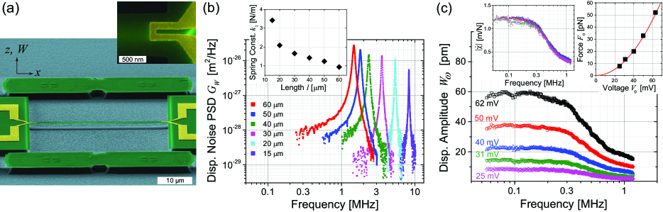
Figure 1: (a) False-colored SEM image of a silicon nitride nanomechanical beam ($l\times b\times h\approx 40~{}\mu\rm m\times 950~{}\rm nm\times 93~{}\rm nm$), showing the structure (green) and the actuators (yellow). (Inset) Close-up image of an electrothermal actuator near one of the clamps of the beam. This is a u-shaped gold film resistor deposited on top of the beam with a thickness of $100~{}\rm nm$ and a width of $120~{}\rm nm$. (b) PSDs of the displacement noise of beams with different lengths ($15~{}{\rm\mu m}\leq l\leq 60~{}{\rm\mu m}$) measured in air around their fundamental resonant modes and at their centers ($x=l/2$). The inset shows the spring constant $k_{1}$ as a function of length for each beam. (c) Driven displacement amplitudes of the 60-$\rm\mu m$-long beam in water at different drive voltages $V_{0}$. Left inset shows the magnitude of the susceptibility $\left|{\hat{\chi}}\right|$ as a function of frequency, and the right inset shows the responsivity of the force transducer. The line is a fit to $F_{0}=A{V_{0}}^{2}$ with $A=1.27\times 10^{-8}~{}\rm N/V^{2}$.

Our experiments are performed on nanomechanical silicon nitride doubly-clamped beam resonators under tension. Figure 1(a) shows a false-colored scanning electron microscope (SEM) image of a typical beam that has dimensions of $l\times b\times h\approx\rm 40~{}\mu m\times 950~{}nm\times 93~{}nm$. There is a 2 $\rm\mu m$ gap between the beam and the substrate. There are two u-shaped metal (gold) electrodes on each end of the beam, through which an AC electric current can be passed (Fig. 1(a) inset). This causes Ohmic heating cycles, which in turn generate thermal bending moments. The result is efficient actuation of nanomechanical oscillations at exactly twice the frequency of the applied AC current [25, 26]. Both the driven and Brownian motions of the beams are measured using a path-stabilized Michelson interferometer that can resolve a displacement of $\sim 5~{}\rm fm/\sqrt{Hz}$ after proper numerical background subtraction [27]. We focus on the out-of-plane motions of the beams at their centers ($x=l/2$), denoted by ${W}(t)$ (Fig. 1(a)). For measurements in liquid, the device chip is immersed in a small bath of liquid. Table 1 lists the dimensions and experimentally-determined mechanical parameters of all the devices used in this study. In the following analysis, we use a density of $\rho_{s}=2750$ kg/m³, Young’s modulus of $E=300$ GPa, and a tension force of $S=7.64$ $\mu$N for all the beams. All experimental details and data are available in the SI [28].

Table 1: Experimentally-obtained mechanical properties of the measured devices.

Device	$l\times b\times h$	$k_{1}$	$m_{1}$	$\omega_{1}/2\pi$
	($\mu\rm m^{3}$)	(N/m)	(pg)	(MHz)
$60\mu\rm m$	$60\times 0.95\times 0.093$	0.93	10.82	1.48
$50\mu\rm m$	$50\times 0.95\times 0.093$	1.24	9.63	1.80
$40\mu\rm m$	$40\times 0.95\times 0.093$	1.42	6.53	2.35
$30\mu\rm m$	$30\times 0.95\times 0.093$	1.66	3.33	3.55
$20\mu\rm m$	$20\times 0.95\times 0.093$	2.09	1.83	5.38
$15\mu\rm m$	$15\times 0.95\times 0.093$	3.42	1.26	8.28

We first describe how the spring constants $k_{1}$ and effective masses $m_{1}$ are obtained for the fundamental mode of the resonators from thermal noise measurements in air. Figure 1(b) shows the PSD of the displacement noise (position fluctuations) $G_{W}$ (in units of $\rm m^{2}/Hz$) at $x=l/2$ as a function of frequency $\frac{\omega}{2\pi}$ for each resonator around its fundamental mode resonance frequency. Since the resonances are sharply-peaked, $G_{W}$ can be integrated accurately over frequency to obtain the mean-squared fluctuation amplitude, $\langle{W}^{2}\rangle$, for the fundamental mode. Using the classical equipartition theorem, we determine the spring constants of the resonators as $k_{1}=k_{B}T/\langle{W}^{2}\rangle$, where $k_{B}$ is the Boltzmann constant and $T$ is the temperature. Thus, $k_{1}$ is the spring constant for the fundamental mode when measured at $x=l/2$. The inset of Fig. 1(b) shows $k_{1}$ as a function of beam length. In air, the frequency of the fundamental mode $\omega_{1}$ and its effective mass $m_{1}$ are assumed to be very close to their respective values in vacuum [29]. Thus, with $k_{1}$ and $\omega_{1}$ in hand, $m_{1}$ can be found from $m_{1}=k_{1}/{\omega_{1}}^{2}$ where $m_{1}$ is the effective mass of the beam in the absence of a surrounding liquid. We discuss how the experimentally measured values of $k_{1}$, $m_{1}$ and $\omega_{1}$ relate to the theoretical predictions for an Euler-Bernoulli beam under tension in the SI [28].

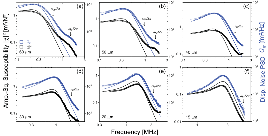
Figure 2: Amplitude-squared susceptibility $\left|{\hat{\chi}}\right|^{2}$ (black) and PSD of the displacement fluctuations $G_{W}$ (blue) for each beam in water; beam length is indicated in the lower left of each panel. Both quantities are measured at the center of the beam $x=l/2$. Square symbols are experimental measurements. The continuous lines are theoretical predictions using the single-mode description. The arrows show the approximate positions of the peaks of the second ($\omega_{2f}/2\pi$) and third mode ($\omega_{3f}/2\pi$) in fluid (when in range).

We now turn to the calibration of the forced response in water. Under a harmonic force $F(t)={F_{0}}\sin{\omega t}$, we can write the oscillatory displacement of the beam at its center as ${W}(t)={{W}_{\omega}}\sin\left({\omega t+{\varphi_{\omega}}}\right)$, with ${W}_{\omega}$ and $\varphi_{\omega}$ being the frequency-dependent displacement amplitude and phase, respectively. Linear response theory yields ${{W}_{\omega}}=\left|{\hat{\chi}(\omega)}\right|{F_{0}}$ [30]. Assuming that the fundamental mode response dominates at low frequency ($\omega\to 0$), one recovers the familiar static (DC) response ${{W}_{dc}}={F_{0}}/{k_{1}}$ (see Eqs. (1) and (2) below). Figure 1(c) shows the driven response of the 60-$\rm\mu m$ beam at $x=l/2$ in water obtained at several different drive voltages. Each data trace is collected by applying to the electrothermal actuator a sinusoidal voltage with constant amplitude $V_{0}$ and sweeping the frequency of the voltage. The displacement amplitude at low frequency, ${W}_{dc}$, is determined from each trace, and $F_{0}$ is found as $F_{0}\approx k_{1}{{W}_{dc}}$ with $k_{1}$ from thermal noise measurements. From the measured displacement amplitudes at different drive amplitudes, one can obtain the force transducer responsivity, shown in the upper right inset of Fig. 1(c). More importantly, under the assumption that $F_{0}$ is constant [28], one can extract the amplitude of the force susceptibility as $\left|{\hat{\chi}(\omega)}\right|\approx{W}_{\omega}/F_{0}$. The left inset of Fig. 1(c) shows that the response of the device at different drive voltages (forces) can be collapsed onto $\left|{\hat{\chi}(\omega)}\right|$ as measured at its center using the proper force calibration.

We show measurements of the driven response and the Brownian fluctuations for each nanomechanical beam in water in Fig. 2. Each double-logarithmic plot corresponds to a separate beam, showing the PSD of the displacement noise, $G_{W}$ (blue, $\rm fm^{2}/Hz$), and the amplitude-squared susceptibility, ${\left|\hat{\chi}\right|^{2}}$ (black, $\rm m^{2}/N^{2}$), as a function of frequency. In all plots, the range shown for both $G_{W}$ and ${\left|\hat{\chi}\right|^{2}}$ are adjusted to span exactly two decades; the ranges of frequency shown are different. The approximate positions of the peaks of the second mode (not detectable at the center of the beam) and the third mode are marked with arrows when in range. Several important observations can be made. It is evident that $G_{W}$ and ${\left|\hat{\chi}\right|^{2}}$ show different frequency dependencies and peak positions. It is precisely these variations that we will use to provide an experimental estimate of the PSD of the Brownian force noise. It is also clear from Fig. 2 that, as the frequency of the fundamental mode increases for the different devices of decreasing length, the overdamped response progressively turns underdamped at higher frequencies where the mass loading due to the fluid is reduced [24].

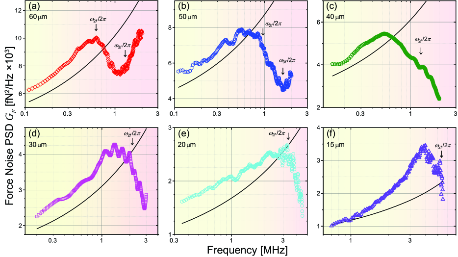
Figure 3: PSD of the Brownian force $G_{F}$ acting on each beam in water. The line is the prediction of Eq. (4) for an oscillating blade in a viscous fluid. Arrows show the higher mode peak positions as in Fig. 2. The shading indicates the approximate frequency region where the fundamental mode is dominant.

The continuous lines in Fig. 2 are from a theoretical description that treats the beams as single-degree-of-freedom harmonic oscillators in a viscous fluid [24]. We first express the linear response function in the familiar general form

$${\left|{\hat{\chi}(\omega)}\right|^{2}}=\frac{1}{{{{\left[{{k_{1}}-{m_{f}}(\omega){\omega^{2}}}\right]}^{2}}+{\omega^{2}}{{\left[{{\gamma_{f}}(\omega)}\right]}^{2}}}}.$$ (1)

The modal mass $m_{f}$ in fluid is a function of frequency due to the mass of fluid that is moving in conjunction with $m_{1}$. In addition, the dissipation due to the viscous fluid $\gamma_{f}$ is frequency dependent. Both $m_{f}(\omega)$ and $\gamma_{f}(\omega)$ can be determined from fluid dynamics by approximating the beam as a long and slender blade (or cylinder) oscillating perpendicular to its axis in a manner consistent with the fundamental mode amplitude profile of the beam [31, 32, 24]. This description yields $\gamma_{f}(\omega)=m_{1}T_{0}\omega\Gamma_{b}^{\prime\prime}({\rm Re}_{\omega})$ and ${m_{f}}(\omega)={m_{1}}\left({1+{T_{0}}\Gamma_{b}^{\prime}({\rm{R}}{{\rm{e}}_{\omega}})}\right)$. The hydrodynamic function of the blade $\Gamma_{b}$ is expressed as a function of the frequency-based Reynolds number, ${\rm Re}_{\omega}=\frac{\omega b^{2}}{4\nu_{f}}$, where $\nu_{f}$ is the kinematic viscosity of the fluid [32, 24]. $\Gamma_{b}$ is a complex valued function, $\Gamma_{b}({\rm Re}_{\omega})=\Gamma_{b}^{\prime}({\rm Re}_{\omega})+i\Gamma_{b}^{\prime\prime}({\rm Re}_{\omega})$, that is determined as an ${\cal O}(1)$ correction to the hydrodynamic function of an oscillating cylinder in fluid [32, 33]. The mass loading parameter, $T_{0}=\frac{\pi\rho_{f}b}{4\rho_{s}h}$, is the ratio of the mass of a cylinder of fluid with diameter $b$ to the mass of the beam, where $\rho_{f}$ and $\rho_{s}$ are fluid and solid densities, respectively. Using these ideas, the amplitude-squared susceptibility can be expressed as [24]

$${\left|{\hat{\chi}(\omega)}\right|^{2}}=\frac{1}{{{{\left[{{k_{1}}-{m_{1}}\left({1+{T_{0}}\Gamma_{b}^{\prime}}\right){\omega^{2}}}\right]}^{2}}+{{{\omega^{2}}\left[{{m_{1}}{T_{0}}\omega\Gamma_{b}^{\prime\prime}}\right]}^{2}}}}$$ (2)

for the fundamental mode of the beam when measured at $x=l/2$. Comparing Eq. (2) with Eq. (1), one can clearly see how the oscillating blade solution provides the parameters for the single-degree-of-freedom harmonic oscillator.

The PSD of the position fluctuations of the fundamental mode of the beam can be expressed as

$$G_{{W}}(\omega)=\left|{\hat{\chi}(\omega)}\right|^{2}G_{F}(\omega).$$ (3)

It follows from the fluctuation-dissipation theorem [34, 35] that the PSD of the Brownian force noise for an oscillating blade or cylinder in fluid can be expressed as [19]

$$G_{F}(\omega)=4k_{B}Tm_{1}T_{0}\omega\Gamma_{b}^{\prime\prime}({\rm Re}_{\omega}).$$ (4)

In Fig. 2, the black lines use Eq. (2) and the blue lines use Eqs. (3-4) where $k_{1}$ and $m_{1}$ are measured from experiment; the force is calibrated using $k_{1}$ at zero frequency; and $\Gamma_{b}$ and $T_{0}$ are calculated from the dimensions and density of the beam and the properties of water. In other words, there are no free fit parameters.

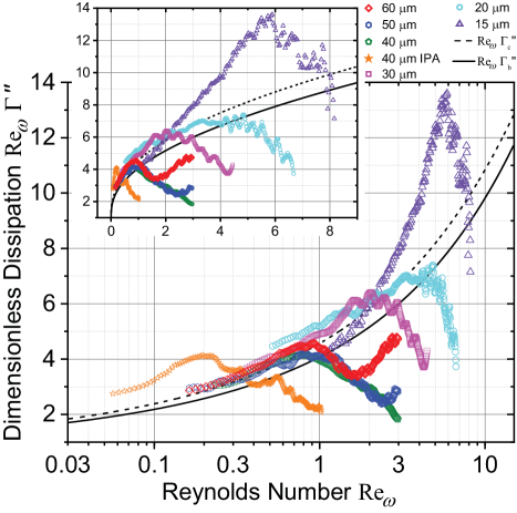
Figure 4: Semi-logarithmic and linear (inset) plots showing all the data in the dimensionless dissipation form. Theoretical predictions are shown for an oscillating cylinder (dashed line) and for an oscillating blade (solid line).

With the displacement noise PSD and the susceptibility experimentally determined, we can find an estimate of the PSD of the Brownian force noise exerted on the beams by the surrounding liquid using $G_{F}(\omega)=G_{W}(\omega)/|\hat{\chi}(\omega)|^{2}$. The symbols in Fig. 3(a)-(f) show the experimentally-obtained PSDs of the Brownian force (in units of $\rm fN^{2}/Hz$) in water. The monotonically-increasing continuous lines are the theoretical predictions for an oscillating blade in a viscous fluid given by Eq. (4). The arrows indicate the approximate peak frequencies, $\omega_{2f}$ and $\omega_{3f}$, of the higher modes as in Fig. 2. The experimental data in Fig. 3(a)-(f) increase with frequency for $\omega\lesssim\omega_{2f}$ as predicted by the theory of an oscillating blade in fluid. However, the experiment begins to deviate from theory around $\omega_{2f}$ for all resonators (Fig. 3(a)-(f)). After making a dip, the data in Fig. 3(a) and (b) begin to increase again around $\omega_{3f}$; this feature remains out of the measurement range in Fig. 3(c)-(f). We attribute these deviations from the theoretical prediction to the influence of the higher modes of oscillation in the driven response of the beam [28], in qualitative agreement with [33].

The general trends of the Brownian force can be made clearer by plotting the experimental data nondimensionally. From Eq. (4), the dimensionless variation of the force PSD can be expressed as ${\rm Re}_{\omega}\Gamma^{\prime\prime}({\rm Re}_{\omega})$. Figure 4 shows ${\rm Re}_{\omega}\Gamma^{\prime\prime}({\rm Re}_{\omega})$ for each data trace in Fig. 3 using semi-logarithmic (main) and linear (inset) plots. To make this plot, we have found experimental $\Gamma^{\prime\prime}$ values from $\Gamma^{\prime\prime}=G_{F}/(4k_{B}Tm_{1}T_{0}\omega$) for each beam, with ${\rm Re}_{\omega}$ acting as a nondimensional frequency. Also shown in Fig. 4 are the theoretical predictions for an oscillating cylinder (dashed line) and blade (solid line) in a viscous fluid. In addition to the six data sets in water, we include data taken in isopropyl alcohol (IPA) [28]. IPA, with its higher viscosity and lower density compared to water, allows us to extend our dimensionless parameter space. The data in Fig. 4 extend over two decades in ${\rm Re}_{\omega}$ and follow the viscous dissipation of a blade (or cylinder) oscillating in the liquid over a range of frequencies.

A more accurate description of the Brownian dynamics of the continuous beams used in the experiments should include the contributions from the higher modes. If we use a multimode lumped description, we can express the PSD of the displacement fluctuations as (cf. Eq. (3))

$$G_{{W}}(\omega)=\sum_{n=1,3,\ldots}^{\infty}|\hat{\chi}_{n}(\omega)|^{2}G_{F,n}(\omega),$$ (5)

where $\hat{\chi}_{n}(\omega)$ represents the susceptibility of the $n^{\rm th}$ mode and the even modes do not contribute since the measurement is at $x=l/2$. Eq. (5) is the sum of the different modal contributions where the modes are assumed to be uncorrelated with one another. For small mode number $n$, a reasonable assumption is that $G_{F,n}(\omega)$ is independent of $n$ to yield $G_{{W}}(\omega)\approx G_{F}(\omega)\sum|\hat{\chi}_{n}(\omega)|^{2}$, where it is clear that the important quantity is the sum of the squares of the susceptibilities of the individual modes.

Similarly, the driven response should be described using a multimode approach that accounts for the spatially-varying aspects of electrothermal drive. This analysis yields an approximate expression of the form

$${{W}_{\omega}}^{2}\approx\bar{\alpha}\left(\pi F_{0}\right)^{2}\left|\sum_{n}\psi_{n}\hat{\chi}_{n}(\omega)\right|^{2}.$$ (6)

Here, $F_{0}$ is the magnitude of the electrothermal force and $\psi_{n}$ accounts for the coupling of the drive to mode $n$ [28]. We have used the fact that magnitude of the odd mode shapes at the center of the beam are nearly constant in order to factor out the constant $\bar{\alpha}\approx\left(\phi_{n}(1/2)\right)^{-2}$ for small and odd $n$, where $\phi_{n}(1/2)$ is the normalized mode shape evaluated at the center of the beam.

Equations (5)-(6) provide some insight into the deviations of the experiment from theory observed in Figs. 3 and 4. For the electrothermal drive applied at the distal ends of the beam, the coefficients $\psi_{n}$ are not expected to be constant and will result in non-trivial contributions from the higher modes. Since, in the single mode approximation, we estimate $G_{F}(\omega)$ by dividing the displacement noise PSD at $\omega$ by the driven response at the same $\omega$, variations in the driven response due to $\psi_{n}$ result in deviations from expected behavior for high frequencies where the influence of the higher modes are significant. We point out that the effects of $\psi_{n}$ cannot be simply deconvoluted or factored out. The electrothermal driven response of the higher modes are entangled due to the large damping in the system, and the driven response becomes quite complicated as the frequency increases. We highlight that Eq. (6) contains the square of the sum whereas Eq. (5) is the sum of the squares. As a result, Eq. (6) would contain complicated contributions due to the cross terms even if the coefficients $\psi_{n}$ could be made nearly constant.

This first direct measurement of the PSD of the Brownian force in a liquid employing nanomechanical resonators is a remarkable manifestation of the fluctuation-dissipation theorem. Even a qualitative explanation of the experimental deviation from theory has required consideration of subtle aspects of the driven response of a continuous system. In the near future, a transducer capable of exerting forces at arbitrary positions with high spatial resolution [36] may allow for directly determining $|\hat{\chi}_{n}(\omega)|^{2}$ for several individual modes. This could then be used to extend the frequency range of the type of measurements described here and would lead to further physical insights into the Brownian force acting on a continuous nanostructure.

ABA and KLE acknowledge support from US NSF through Grant Nos. CBET-1604075 and CMMI-2001403. MRP acknowledges support from US NSF Grant No. CMMI-2001559.

References

- Chandler [1987] D. Chandler, Introduction to Modern Statistical Mechanics, 1st ed. (Oxford University Press, New York, 1987).
- Kubo et al. [1985] R. Kubo, M. Toda, and N. Hashitsume, Statistical Physics II: Nonequilibrium Statistical Mechanics, 2nd ed., Vol. 31 (Springer, Heidelberg, 1985).
- Franosch et al. [2011] T. Franosch, M. Grimm, M. Belushkin, F. M. Mor, G. Foffi, L. Forró, and S. Jeney, Resonances arising from hydrodynamic memory in Brownian motion, Nature 478, 85 (2011).
- Jannasch et al. [2011] A. Jannasch, M. Mahamdeh, and E. Schäffer, Inertial effects of a small brownian particle cause a colored power spectral density of thermal noise, Physical Review Letters 107, 228301 (2011).
- Cohadon et al. [1999] P. F. Cohadon, A. Heidmann, and M. Pinard, Cooling of a mirror by radiation pressure, Physical Review Letters 83, 3174 (1999).
- Gillespie and Raab [1995] A. Gillespie and F. Raab, Thermally excited vibrations of the mirrors of laser interferometer gravitational-wave detectors, Physical Review D 52, 577 (1995).
- Adhikari [2014] R. X. Adhikari, Gravitational radiation detection with laser interferometry, Reviews of Modern Physics 86, 121 (2014).
- Bunch et al. [2007] J. S. Bunch, A. M. Van Der Zande, S. S. Verbridge, I. W. Frank, D. M. Tanenbaum, J. M. Parpia, H. G. Craighead, and P. L. McEuen, Electromechanical resonators from graphene sheets, Science 315, 490 (2007).
- Barnard et al. [2019] A. W. Barnard, M. Zhang, G. S. Wiederhecker, M. Lipson, and P. L. McEuen, Real-time vibrations of a carbon nanotube, Nature 566, 89 (2019).
- Cleland and Roukes [1998] A. N. Cleland and M. L. Roukes, A nanometre-scale mechanical electrometer, Nature 392, 160 (1998).
- Ekinci et al. [2004] K. L. Ekinci, X. M. Huang, and M. L. Roukes, Ultrasensitive nanoelectromechanical mass detection, Applied Physics Letters 84, 4469 (2004).
- Aspelmeyer et al. [2014] M. Aspelmeyer, T. J. Kippenberg, and F. Marquardt, Cavity optomechanics, Reviews of Modern Physics 86, 1391 (2014).
- O’Connell et al. [2010] A. D. O’Connell, M. Hofheinz, M. Ansmann, R. C. Bialczak, M. Lenander, E. Lucero, M. Neeley, D. Sank, H. Wang, M. Weides, J. Wenner, J. M. Martinis, and A. N. Cleland, Quantum ground state and single-phonon control of a mechanical resonator, Nature 464, 697 (2010).
- Cleland [2003] A. N. Cleland, Foundations of Nanomechanics (Springer Berlin Heidelberg, Berlin, 2003).
- Saulson [1990] P. R. Saulson, Thermal noise in mechanical experiments, Physical Review D 42, 2437 (1990).
- Cleland and Roukes [2002] A. N. Cleland and M. L. Roukes, Noise processes in nanomechanical resonators, Journal of Applied Physics 92, 2758 (2002).
- Majorana and Ogawa [1997] E. Majorana and Y. Ogawa, Mechanical thermal noise in coupled oscillators, Physics Letters, Section A: General, Atomic and Solid State Physics 233, 162 (1997).
- Schwarz et al. [2016] C. Schwarz, B. Pigeau, L. Mercier De Lépinay, A. G. Kuhn, D. Kalita, N. Bendiab, L. Marty, V. Bouchiat, and O. Arcizet, Deviation from the Normal Mode Expansion in a Coupled Graphene-Nanomechanical System, Physical Review Applied 6, 064021 (2016).
- Paul and Cross [2004] M. R. Paul and M. C. Cross, Stochastic dynamics of nanoscale mechanical oscillators immersed in a viscous fluid, Physical Review Letters 92, 235501 (2004).
- Mo et al. [2015] J. Mo, A. Simha, and M. G. Raizen, Broadband boundary effects on Brownian motion, Physical Review E - Statistical, Nonlinear, and Soft Matter Physics 92, 062106 (2015).
- Miao et al. [2012] H. Miao, K. Srinivasan, and V. Aksyuk, A microelectromechanically controlled cavity optomechanical sensing system, New Journal of Physics 14, 10.1088/1367-2630/14/7/075015 (2012).
- Teufel et al. [2009] J. D. Teufel, T. Donner, M. A. Castellanos-Beltran, J. W. Harlow, and K. W. Lehnert, Nanomechanical motion measured with an imprecision below that at the standard quantum limit, Nature Nanotechnology 4, 820 (2009).
- Doolin et al. [2014] C. Doolin, P. H. Kim, B. D. Hauer, A. J. R. MacDonald, and J. P. Davis, Multidimensional optomechanical cantilevers for high-frequency force sensing, New Journal of Physics 16, 10.1088/1367-2630/16/3/035001 (2014).
- Paul et al. [2006] M. R. Paul, M. T. Clark, and M. C. Cross, The stochastic dynamics of micron and nanoscale elastic cantilevers in fluid: Fluctuations from dissipation, Nanotechnology 17, 4502 (2006), 0605035 .
- Ari et al. [2018] A. B. Ari, M. Cagatay Karakan, C. Yanik, I. I. Kaya, and M. Selim Hanay, Intermodal Coupling as a Probe for Detecting Nanomechanical Modes, Physical Review Applied 9, 034024 (2018).
- Bargatin et al. [2007] I. Bargatin, I. Kozinsky, and M. L. Roukes, Efficient electrothermal actuation of multiple modes of high-frequency nanoelectromechanical resonators, Applied Physics Letters 90, 1 (2007).
- Kara et al. [2015] V. Kara, Y. I. Sohn, H. Atikian, V. Yakhot, M. Lončar, and K. L. Ekinci, Nanofluidics of Single-Crystal Diamond Nanomechanical Resonators, Nano Letters 15, 8070 (2015).
- [28] See Supplemental Material for additional details on device properties and theoretical derivations.
- Kara et al. [2017] V. Kara, V. Yakhot, and K. L. Ekinci, Generalized Knudsen Number for Unsteady Fluid Flow, Physical Review Letters 118, 10.1103/PhysRevLett.118.074505 (2017), arXiv:1702.07783 .
- Sethna [2006] J. Sethna, Statistical Mechanics: Entropy, Order Parameters, and Complexity (OUP Oxford, Oxford, 2006).
- Rosenhead [1963] L. Rosenhead, Fluid Motion Memoirs: Laminar Boundary Layers, 1st ed. (Oxford University Press, Oxford, 1963).
- Sader [1998] J. E. Sader, Frequency response of cantilever beams immersed in viscous fluids with applications to the atomic force microscope, Journal of Applied Physics 84, 64 (1998).
- Clark et al. [2010] M. T. Clark, J. E. Sader, J. P. Cleveland, and M. R. Paul, Spectral properties of microcantilevers in viscous fluid, Physical Review E - Statistical, Nonlinear, and Soft Matter Physics 81, 046306 (2010).
- Callen and Welton [1951] H. B. Callen and T. A. Welton, Irreversibility and generalized noise, Physical Review 83, 34 (1951).
- Callen and Greene [1952] H. B. Callen and R. F. Greene, On a theorem of irreversible thermodynamics, Physical Review 86, 702 (1952).
- Sampathkumar et al. [2006] A. Sampathkumar, T. W. Murray, and K. L. Ekinci, Photothermal operation of high frequency nanoelectromechanical systems, Applied Physics Letters 88, 223104 (2006).