Adiabatically Induced Orbital Magnetization

Abstract

A semiclassical theory for the orbital magnetization due to adiabatic evolutions of Bloch electronic states is proposed. It renders a unified theory for the periodic-evolution pumped orbital magnetization and the orbital magnetoelectric response in insulators by revealing that these two phenomena are the only instances where the induced magnetization is gauge invariant. This theory also accounts for the electric-field induced intrinsic orbital magnetization in two-dimensional metals and Chern insulators. We illustrate the orbital magnetization pumped by microscopic local rotations of atoms, which correspond to phonon modes with angular momentum, in toy models based on honeycomb lattice, and the results are comparable to the pumped spin magnetization via strong Rashba spin orbit coupling. We also show the vital role of the orbital magnetoelectricity in validating the Mott relation between the intrinsic nonlinear anomalous Hall and Ettingshausen effects.

I Introduction

Understanding the orbital magnetization in crystalline solids is among the most important objectives of orbitronics Zhang2005 ; Go2017 ; Bhowal2020 . Unlike its spin companion, the orbital magnetization of Bloch electrons in the absence of external perturbations is already hard to access quantum mechanically, as it does not correspond to a bounded operator. This nonlocality is finally accounted for by a Berry phase formula Xiao2005 ; Resta2005 ; Shi2007 that gives significantly distinct orbital magnetization from the atom-centered approximation when combined with ab-initio calculations in various magnetic materials Ceresoli2010 ; Lopez2012 ; Hanke2016 . In the presence of external driving electric fields, the extrinsic responses of spin and orbital magnetization, namely the spin and orbital Edelstein effects, are given similarly by the magnetic moments averaged over current-carrying states Edelstein1990 ; Murakami2015 ; Mak2017 ; Pesin2018 ; Salemi2019 ; Mertig2020 . In contrast, the intrinsic responses of them, i.e., the spin and orbital magnetoelectric effects, are completely different due to the nonlocal nature of the magnetic dipole operator. Specifically, the spin magnetoelectricity Garate2009 ; Garate2010 is dictated by a Berry curvature following the ubiquitous character of intrinsic linear responses of a local operator Dong2020 , while the orbital one consists of a Chern-Simons three form and a perturbative term of the reciprocal-space Berry connection Moore2010 ; Vanderbilt2010 ; Lee2011 ; Gao2014 . Besides, the magnetization pumped by periodic adiabatic processes in band insulators has been studied recently by a density matrix approach evaluating the time-averaged expectation value of the spin and magnetic dipole operators Luka2019 ; Murakami2020 . In this approach, the orbital magnetization can only be obtained in the Wannier basis Luka2019 , in contrast to the spin one that can be evaluated in the Bloch representation.

Up to date, the orbital magnetization induced by electric fields and by periodic adiabatic processes are treated by different theories. Whether both phenomena have a deep connection and if they can emerge in a unified theoretical framework are still unknown. In this work, we develop a semiclassical theory for the magnetization induced by adiabatic evolutions of Bloch electronic states. In general, the adiabatically induced orbital magnetization is gauge dependent due to the presence of the electric current in the second Chern form of Berry curvatures. Noticeably, the orbital magnetoelectric effect and the periodic-evolution pumped orbital magnetization emerge as the only instances where the induced magnetization is gauge invariant due to the elimination of its explicit time dependence. Our work thus renders a unified theory of both phenomena in insulators with vanishing Chern numbers. Besides, unlike the Chern-Simons contribution deduced from the second Chern form current, the induced magnetization due to the perturbed Berry connection is well defined irrespective of Chern invariants and of insulators or metals. As a result, the orbital magnetoelectricity in two-dimensional (2D) metals and Chern insulators, which had long been hard to approach, is also attained in our theory.

We apply our theory to illustrate the orbital magnetization pumped by microscopic atomic rotations, which correspond to phonon modes with angular momentum Zhang2014 ; Garanin2015 , in toy models based on the honeycomb lattice. The results are comparable to the pumped spin magnetization via a strong Rashba spin orbit coupling Murakami2020 . We also show the vital role played by the electric-field induced orbital magnetization in the nonlinear intrinsic anomalous Ettingshausen effect in 2D metallic systems. In particular, the Mott relation is validated in intrinsic nonlinear transport by subtracting the magnetization component of the thermal current in the second order of the electric field.

This paper is organized as follows. In Sec. II we lay out the semiclassical theory of Bloch electrons, which is employed to study the adiabatically induced orbital magnetization in metals and insulators, respectively, in Sec. III and Sec. IV. A case study of the orbital magnetization pumped by local rotations of atoms and the application of the orbital magnetoelectricity to the intrinsic nonlinear anomalous Ettingshausen effect are shown in Sec. V, followed by a summary in Sec. VI. Some technical details of the theory are presented in Appendices A and B for the convenience of interested readers.

II Semiclassical theory

In the semiclassical description, the Hamiltonian felt by a narrow wave packet centered around position $\bm{r}_{c}$ is $\hat{H}=\hat{H}_{c}+\hat{H}^{\prime}$ in the first order gradient expansion, where $\hat{H}_{c}=\hat{H}_{0}\left(\bm{\hat{r}},\bm{\hat{p}};w\left(\bm{r}_{c}\right),R\left(t\right)\right)+\sum_{\alpha}\bm{\hat{\theta}}^{\left(\alpha\right)}\cdot\bm{h}^{\left(\alpha\right)}\left(\bm{r}_{c},t\right)\$is the local Hamiltonian and $\hat{H}^{\prime}=\frac{1}{2}\{\left(\hat{r}-r_{c}\right)_{i},\frac{\partial\hat{H}_{c}}{\partial r_{ci}}\}$ is the gradient correction Sundaram1999 . The Einstein summation convention is implied for repeated Cartesian indices $i$, $j$ and $s$ henceforth. $\hat{H}_{0}$ is the local approximation of the genuine Hamiltonian. The most general $\hat{H}_{0}$ considered here includes $w\left(\bm{r}_{c}\right)$ that represents possible nonuniform static mechanical fields varying slowly on the scale of the wave packet as well as $R\left(t\right)$ serving as a parameter whose time evolution is adiabatic. Besides, in order to implement the variational approach to obtain the local density of a bounded observable, we add the auxiliary term $\sum_{\alpha}\bm{\hat{\theta}}^{\left(\alpha\right)}\cdot\bm{h}^{\left(\alpha\right)}\left(\bm{r},t\right)$ into the Hamiltonian and expand it around $\bm{r}_{c}$. Here $\bm{\hat{\theta}}^{\left(\alpha\right)}$ ($\alpha=1,2,..$) is a set of bounded observable operators, each of which is assumed to be a vector for simple notations, without losing generality. $\bm{h}^{\left(\alpha\right)}\left(\bm{r},t\right)$ denotes the conjugate slowly varying external fields, and $\bm{h}^{\left(\alpha\right)}\left(\bm{r}_{c},t\right)$ changes adiabatically in the parameter space $\left(t,\bm{r}_{c}\right)$. At the end of the calculation the auxiliary term is set to zero, i.e., $\bm{h}^{\left(\alpha\right)}=0$.

In the semiclassical theory that is accurate to the first order of spatial gradients and of time derivative Sundaram1999 ; Xiao2010 , the wave packet $|W_{n}\left(\bm{k},\bm{r}_{c},t\right)\rangle=\sum_{\bm{p}}C_{n\bm{p}}|\psi_{n\bm{p}}\rangle$ is constructed by superposing the local Bloch states $|\psi_{n\bm{p}}\left(\bm{r}_{c},t\right)\rangle=e^{i\bm{p}\cdot\bm{\hat{r}}}|u_{n\bm{p}}\left(\bm{r}_{c},t\right)\rangle$ of $\hat{H}_{c}$. Here $n$ and $\hbar\bm{p}$ are the band index and crystal momentum, respectively, and the coefficient $C_{n\bm{p}}$ is sharply distributed around the wave vector $\bm{k}$ of the wave packet, obeying $\sum_{\bm{p}}\left|C_{n\bm{p}}\right|^{2}=1$. To simplify notations, all the band quantities without explicit band index are considered for band $n$, unless otherwise noted. Throughout this study we consider nondegenerate bands to simplify the analysis and assume they are so separated that adiabatic evolutions are feasible. The wave packet Lagrangian reads (set $\hbar=1$)

$$L=\langle W|i\frac{d}{dt}-\hat{H}|W\rangle=\bm{\dot{r}}_{c}\cdot\bm{k}+\bm{\dot{k}}\cdot\bm{\mathcal{A}}^{k}+\bm{\dot{r}}_{c}\cdot\bm{\mathcal{A}}^{r_{c}}+\mathcal{A}^{t}-\tilde{\varepsilon},$$ (1)

where $\bm{\mathcal{A}}^{k/r_{c}}=\langle u_{n}|i\partial_{\bm{k/r}_{c}}\mathbf{|}u_{n}\rangle$ and $\mathcal{A}^{t}=\langle u_{n}|i\partial_{t}\mathbf{|}u_{n}\rangle$ are the Berry connections derived from the periodic part $|u_{n}\left(\bm{k},\bm{r}_{c},t\right)\rangle$ of the Bloch wave Sundaram1999 . The noncanonical form of the Lagrangian due to Berry connections implies that $\left(\bm{r}_{c},\bm{k}\right)$ are not canonical variables, thus the measure of the phase space spanned by $\left(\bm{r}_{c},\bm{k}\right)$ should be modified, with the result Xiao2005 $\mathcal{D}=1+\Omega_{ii}^{kr_{c}}$. Here $\Omega_{ii}^{kr_{c}}$ is the trace of the Berry curvature $\Omega_{ij}^{kr_{c}}\equiv\partial_{k_{i}}\mathcal{A}_{j}^{r_{c}}-\partial_{r_{cj}}\mathcal{A}_{i}^{k}$, and other Berry curvatures are formed similarly. The wave-packet energy is given by $\tilde{\varepsilon}=\varepsilon+\delta\varepsilon$ up to first order gradients, where $\varepsilon_{n}\left(\bm{k},\bm{r}_{c},t\right)$ is the local Bloch energy, $\delta\varepsilon_{n}=\operatorname{Re}\sum_{n_{1}\neq n}\bm{\mathcal{A}}_{nn_{1}}^{k}\cdot(\partial_{\bm{r}_{c}}\hat{H}_{c})_{n_{1}n}$ and $\bm{\mathcal{A}}_{nn_{1}}^{k}=\langle u_{n}|i\partial_{\bm{k}}\mathbf{|}u_{n_{1}}\rangle$ is the interband Berry connection.

When going beyond the above first-order theory, the wave packet is no longer dictated only by the Bloch states of local Hamiltonian $\hat{H}_{c}$ but is modified by $\hat{H}^{\prime}$ up to the linear order of spatial gradients Gao2014 . In the well established second-order theory Gao2019 the inhomogeneity appears only in electromagnetic gauge potentials, whereas the following results account for weak inhomogeneities of mechanical fields conjugate to general bounded operators. This generalization is necessary to obtain the adiabatically induced orbital magnetization carried by Bloch electrons by calculating the magnetization current, which is manifested only in nonuniform systems Cooper1997 ; Xiao2020EM . For this purpose, it is sufficient to retain results up to the order of the product spatial and time derivatives.

In the second-order theory the wave packet takes the form of Gao2019

$$|W_{n}\left(\bm{k},\bm{r}_{c},t\right)\rangle=\sum_{\bm{p}}e^{i\bm{p}\cdot\bm{\hat{r}}}[C_{n\bm{p}}|u_{n\bm{p}}\rangle+\sum_{n_{1}\neq n}C_{n_{1}\bm{p}}|u_{n_{1}\bm{p}}\rangle],$$ (2)

where (derivations presented in Appendix A)

$$C_{n_{1}}=\frac{\Delta_{n_{1}n}C_{n}}{\varepsilon_{n\bm{p}}-\varepsilon_{n_{1}\bm{p}}}-i\bm{\mathcal{A}}_{n_{1}n}^{r_{c}}\cdot(i\partial_{\bm{p}}+\bm{\mathcal{A}}_{n}^{p}-\bm{r}_{c})C_{n}$$ (3)

incorporates spatial-gradient induced corrections. Here

$$\Delta_{n_{1}n} \equiv\frac{i}{2}(\partial_{\bm{\hat{p}}}\cdot\partial_{\bm{r}_{c}}\hat{H}_{c})_{n_{1}n}+\sum_{n_{2}\neq n}(\partial_{\bm{r}_{c}}\hat{H}_{c})_{n_{1}n_{2}}\cdot\bm{\mathcal{A}}_{n_{2}n}^{p}$$

$$-\bm{\mathcal{A}}_{n_{1}n}^{r_{c}}\cdot\bm{v}_{n}$$ (4)

has the dimension of energy, with $\bm{\mathcal{A}}_{nn_{1}}^{r_{c}}=\langle u_{n}|i\partial_{\bm{r}_{c}}\mathbf{|}u_{n_{1}}\rangle$. The wave-packet center appearing in Eq. (3) is determined by $\bm{r}_{c}=\langle W|\bm{\hat{r}}|W\rangle=\partial_{\bm{k}}\gamma(\bm{k})+\bm{\mathcal{A}}^{k}+\bm{a}^{k}$, where $-\gamma(\bm{p})$ is the phase of $C_{n\bm{p}}$. While the first two terms appear already in the first order theory Sundaram1999 , the third term $\bm{a}_{n}^{k}\equiv 2\operatorname{Re}\sum_{\bm{p}}\sum_{n_{1}\neq n}C_{n\bm{p}}^{\ast}C_{n_{1}\bm{p}}\bm{\mathcal{A}}_{nn_{1}}^{p}$ is the inhomogeneity induced positional shift of the wave-packet center. Gathering the above results we get a gauge invariant expression

$$\bm{a}_{n}^{k}=2\operatorname{Re}\sum_{n_{1}\neq n}\frac{\bm{\mathcal{A}}_{nn_{1}}^{k}\Delta_{n_{1}n}}{\varepsilon_{n}-\varepsilon_{n_{1}}}-\partial_{\bm{k}}\cdot\mathcal{G}_{n}^{r_{c}k},$$ (5)

with $\mathcal{G}_{n}^{r_{c}k}=\operatorname{Re}\sum_{n_{1}\neq n}\bm{\mathcal{A}}_{nn_{1}}^{r_{c}}\bm{\mathcal{A}}_{n_{1}n}^{k}$ being the quantum metric tensor in $\left(\bm{r}_{c},\bm{k}\right)$ space.

One can then find that the wave-packet Lagrangian takes the same form [Eq. (1)] as in the first order theory, but the involved Berry connections are modified by inhomogeneity, i.e., $\bm{\mathcal{\tilde{A}}}^{k}=\bm{\mathcal{A}}^{k}+\bm{a}^{k}$ and $\mathcal{\tilde{A}}^{t}=\mathcal{A}^{t}+a^{t}$. The corrected Berry connections in fact take similar structures, e.g.,

$$a_{n}^{t}=2\operatorname{Re}\sum_{n_{1}\neq n}\frac{\mathcal{A}_{nn_{1}}^{t}\Delta_{n_{1}n}}{\varepsilon_{n}-\varepsilon_{n_{1}}}-\partial_{\bm{k}}\cdot\bm{\mathcal{G}}_{n}^{r_{c}t},$$ (6)

where $\bm{\mathcal{G}}_{n}^{r_{c}t}=\operatorname{Re}\sum_{n_{1}\neq n}\bm{\mathcal{A}}_{nn_{1}}^{r_{c}}\mathcal{A}_{n_{1}n}^{t}$, and are gauge invariant. Note that the correction to $\bm{\mathcal{A}}^{r_{c}}$ is not needed, since $\bm{\mathcal{A}}^{r_{c}}$ is already in the first order of spatial gradients. Meanwhile, the wave-packet energy does not receive further corrections at the order of the product spatial and time derivatives.

Having identified the wave-packet Lagrangian and the concomitant action $S$, one gets directly the semiclassical dynamics of Bloch electrons following from the Euler-Lagrange equation in $\left(\bm{r}_{c},\bm{k}\right)$ space. Furthermore, one can consider the local density of a bounded observable $\bm{\hat{\theta}}$, of which the conjugate external field is marked by $\bm{h}$, contributed by a Bloch-electron ensemble with the occupation function $f_{n}\left(\bm{r}_{c},\bm{k},t\right)$. The general recipe for this has been given recently as Dong2020

$$\bm{\theta}\left(\bm{r},t\right)=-\int\left[d\bm{k}\right]d\bm{r}_{c}\mathcal{D}f\frac{\delta S}{\delta\bm{h}\left(\bm{r},t\right)}|_{\bm{h}\rightarrow 0},$$ (7)

where $\left[d\bm{k}\right]\equiv\sum_{n}d\bm{k}/(2\pi)^{d}$ with $d$ as the spatial dimensionality. In what follows we suppress the notation $\bm{h}\rightarrow 0$ but the results for various adiabatic responses are calculated in this limit. We take $f(\tilde{\varepsilon})$ as the Fermi distribution in order to focus on adiabatic intrinsic contributions determined solely by band structures.

The spin magnetoelectricity and spin pumping by periodic adiabatic processes can be readily obtained from the above formula in the first order of time derivative, as detailed in Appendix B, while the orbital counterparts can only be acquired through calculating the electric current, which is much more involved and is elaborated in the next two sections.

III Orbital magnetization in metals

III.1 Nonlinear electric current

In order to address the orbital magnetization induced by adiabatic evolutions, we need to formulate the local charge current density up to the order of the product spatial and time derivatives. To achieve this Eq. (7) is considered in the case of $\bm{\hat{\theta}}=e\bm{\hat{v}}$ being the charge current operator, hence $\bm{h}=-\bm{A}$ is the electromagnetic vector potential with a minus sign, which enters through the minimal coupling, resulting in the chain rule $\partial_{-\bm{A}}=e\partial_{\bm{k}}$. We still use $\bm{k}$ to denote the gauge invariant crystal momentum. In the following the center label $c$ is suppressed, unless otherwise noted. After some manipulations, as shown in Appendix B, we arrive at (hereafter $\int$ without integral variable is shorthand for $\int\left[d\bm{k}\right]$, $f^{0}=f\left(\varepsilon\right)$)

$$\bm{j}\left(\bm{r},t\right) =\bm{\nabla}\times(\bm{M}^{0}+\int f^{0}\partial_{\bm{B}}a^{t})+\partial_{t}\int f^{0}e\bm{a}^{k}$$

$$-e\int f^{0}(\Omega^{\bm{k}t}+\Omega_{s}^{k\left[kr\right]t}\bm{\hat{e}}_{s})$$

$$-e\int\partial_{\varepsilon}f^{0}\delta\varepsilon\Omega^{\bm{k}t}+e\int(\partial_{\bm{k}}f^{0}a^{t}-\partial_{t}f^{0}\bm{a}^{k}),$$ (8)

where the second Chern form of the Berry curvature Xiao2009 ; Zhou2013 is labeled as

$$\Omega_{s}^{k\left[kr\right]t}\equiv\Omega_{si}^{kk}\Omega_{i}^{rt}+\Omega_{si}^{kr}\Omega_{i}^{tk}+\Omega_{s}^{kt}\Omega_{ii}^{kr},$$ (9)

$\bm{\hat{e}}_{s}$ is the unit vector in the $s$ direction, and

$$\bm{M}^{0}=\int(f^{0}\bm{m}+eg^{0}\bm{\Omega}).$$ (10)

Here $\bm{m}_{n}=\frac{e}{2}\sum_{n_{1}\neq n}\bm{\mathcal{A}}_{nn_{1}}^{k}\times\bm{v}_{n_{1}n}$ is the orbital moment of a Bloch electron, $\bm{\Omega}$ is the vector form of Berry curvature $\Omega_{ij}^{kk}$, and $g^{0}=-\int_{\varepsilon}^{\infty}f(\eta)d\eta$ is the grand potential density contributed by a Bloch electron. With the symmetric gauge for the uniform magnetic field, Eq. (6) gives

$$\partial_{\bm{B}}a^{t}=2\operatorname{Re}\sum_{n_{1}\neq n}\frac{-\mathcal{A}_{nn_{1}}^{t}\bm{m}_{n_{1}n}}{\varepsilon_{n}-\varepsilon_{n_{1}}}+\frac{e}{2}\partial_{\bm{k}}\times\bm{\mathcal{G}}_{n}^{kt},$$ (11)

where $\bm{\mathcal{G}}_{n}^{kt}=\operatorname{Re}\sum_{n_{1}\neq n}\bm{\mathcal{A}}_{nn_{1}}^{k}\mathcal{A}_{n_{1}n}^{t}$ is the quantum metric in $\left(\bm{k},t\right)$ space, and $\bm{m}_{n_{1}n}=-\partial_{\bm{B}}\Delta_{n_{1}n}$, which will be elaborated later in combination with a more specific physical context.

Equation (8) is the pivotal result of this paper. The first line is of total spatial and time derivatives, hence is certainly intimately related to the orbital magnetization and electric polarization. Apparently, $\bm{M}^{0}$ is the magnetization that relies solely on instantaneous electronic states and corresponds to the equilibrium orbital magnetization in the static case Shi2007 . On the other hand, the magnetization and polarization may not be determined by the first line of Eq. (8) alone, as the second line can be relevant as well. This line consists of first and second Chern forms of Berry curvatures, which underline various electronic topological responses of insulators Xiao2009 ; Xiao2010 ; Qi2008 ; Essin2009 . Besides, the last line signifies intrinsic Fermi-surface contributions to the charge current density in metals, which are beyond the conventional Boltzmann transport picture of conductors Ziman and are distinct from intrinsic Fermi-sea contributions to linear response.

Now we are in a position to compare Eq. (8) with existing results at the same order. The second line of this equation has been formulated in inhomogeneous insulators Xiao2009 ; Qi2015 and metals Hayata2017 . The specific case where the inhomogeneity enters only through the magnetic vector potential has been studied in insulators with degenerate bands Moore2010 ; Qi2008 and in metals Moore2016 . Meanwhile, these pioneering studies disregarded the magnetization current in the first line of Eq. (8), especially the orbital magnetization induced by the Berry connection $a^{t}$ due to adiabatic time evolutions [Eq. (11)]. However, there is an important physical context: orbital magnetoelectricity in 2D metals, which is contributed entirely by this gauge invariant term and hence is beyond the scope of the aforementioned theories. We discuss this subject shortly.

III.2 Orbital magnetoelectricity in 2D

To address the orbital magnetoelectricity, we consider the case that the adiabatic time dependence stems entirely from the vector potential, i.e., $\bm{E}=-\partial_{t}\bm{A}$, with $\bm{E}$ being a weak constant electric field, then $\partial_{t}=e\bm{E}\cdot\partial_{\bm{k}}$, $a^{t}=\bm{a}^{k}\cdot e\bm{E}$ and $\Omega_{s}^{k\left[kr\right]t}=\Omega_{sj}^{k\left[kr\right]k}eE_{j}$. Thus the local charge current density [Eq. (8)] reduces to

$$\bm{j}\left(\bm{r}\right) =\bm{\nabla}\times[\bm{M}^{0}+\int f^{0}\partial_{\bm{B}}(e\bm{E\cdot a}^{k})]$$

$$-e^{2}\bm{E}\times\int f^{0}\bm{\Omega}-e^{2}E_{i}\int f^{0}\Omega_{si}^{k\left[kr\right]k}\bm{\hat{e}}_{s}$$

$$+e^{2}\bm{E}\times\int\partial_{\varepsilon}f^{0}(\bm{v}\times\bm{a}^{k}-\delta\varepsilon\bm{\Omega}).$$ (12)

To understand this current we first inspect the case when the spatial dependence originates only from the vector potential, i.e., $\bm{B}=\bm{\nabla}\times\bm{A}$. Then it is apparent that

$$\bm{j}=-e^{2}\bm{E}\times\int\{f^{0}\bm{\Omega}-\partial_{\varepsilon}f^{0}[\bm{v}\times(\bm{a}^{k})^{\bm{B}}+\left(\bm{m}\cdot\bm{B}\right)\bm{\Omega}]\},$$ (13)

where $(\bm{a}^{k})^{\bm{B}}$ is proportional to the magnetic field. This result recovers the intrinsic magneto-nonlinear Hall current of order $EB$ that was obtained previously by a different method Gao2014 .

On the other hand, to identify the orbital magnetization one could introduce the spatial dependence from other inhomogeneous external mechanical fields. By doing so one may expect that the local current density in bulk can be decomposed into a transport and a magnetization component, namely Cooper1997

$$\bm{j}=\bm{j}^{\text{tr}}+\bm{\nabla}\times\bm{M},$$ (14)

where the transport current $\bm{j}^{\text{tr}}$ contributes to the net flow through the sample. In 2D the second Chern form current is enforced to vanish due to $\Omega_{si}^{k\left[kr\right]k}=0$, hence Eq. (14) is rescued with $\bm{j}^{\text{tr}}$ taking the same form as the above magneto-nonlinear Hall current Eq. (13) and

$$\bm{M}=\bm{M}^{0}+\int f^{0}\partial_{\bm{B}}(e\bm{E\cdot a}^{k}).$$ (15)

Recall that $\bm{a}^{k}$ is physically a positional shift of a semiclassical Bloch electron, the electric work upon this shift implies immediately an orbital magnetization. This electric-field induced magnetization is in agreement with what is obtained recently by a different method Xiao2020OM , but the present derivation is much simpler, even though starting from a more generic framework. In 2D, $\bm{M}$ is a pseudoscalar and is well defined irrespective of metals or Chern insulators.

Owing to the gauge invariance of $\bm{a}^{k}$, it is legitimate to define the orbital magnetoelectric susceptibility contributed by each Bloch electron in 2D $\alpha_{ij}^{\text{o}}$ via

$$\partial M_{j}/\partial E_{i}=\int f^{0}\alpha_{ij}^{\text{o}}.$$ (16)

$\alpha_{ij}^{\text{o}}$ takes a gauge invariant form ($j=z$ in 2D)

$$\alpha_{ij}^{\text{o}}=-2e\operatorname{Re}\sum_{n_{1}\neq n}\frac{(\mathcal{A}_{i}^{k})_{nn_{1}}(m_{j})_{n_{1}n}}{\varepsilon_{n}-\varepsilon_{n_{1}}}+\frac{e^{2}}{2}\epsilon_{jls}\partial_{k_{l}}(\mathcal{G}_{si}^{kk})_{n},$$ (17)

with $\mathcal{G}_{n}^{kk}=\operatorname{Re}\sum_{n_{1}\neq n}\bm{\mathcal{A}}_{nn_{1}}^{k}\bm{\mathcal{A}}_{n_{1}n}^{k}$ as the $\bm{k}$-space quantum metric QM2020 .

It is interesting to compare $\alpha_{ij}^{\text{o}}$ with the spin magnetoelectric susceptibility contributed by each Bloch electron, which is given by the first term of Eq. (17) with $\bm{m}_{n_{1}n}$ replaced by the interband elements of spin magnetic moment. Since $\bm{m}_{n_{1}n}=-\frac{e}{2}\sum_{n_{2}\neq n}(\bm{v}_{n_{1}n_{2}}+\delta_{n_{2}n_{1}}\bm{v}_{n})\times\bm{\mathcal{A}}_{n_{2}n}^{k}$ reduces to the familiar orbital moment $\bm{m}_{n}$ when $n_{1}=n$, it can be deemed as an interband orbital magnetic moment. Despite this similarity between spin and orbital magnetoelectric susceptibility, the distinction is apparent: the $\bm{k}$-space dipole moment of the quantum metric $\partial_{k_{l}}\mathcal{G}_{si}^{kk}$ does not have a counterpart in spin magnetoelectricity. Noticeably, for two-band metallic systems with particle-hole symmetry, the first term of $\alpha_{ij}^{\text{o}}$ vanishes, hence $\alpha_{ij}^{\text{o}}=\frac{e^{2}}{2}\epsilon_{jls}\partial_{k_{l}}\mathcal{G}_{si}^{kk}$ is given solely by the quantum metric dipole, which is an intrinsic Fermi surface effect.

Before closing this section, we note that in 3D insulators with nonvanishing $\bm{k}$-space Chern invariants or 3D metals, the second Chern form current in Eq. (12) obviously poses a difficulty in pursuing a gauge invariant decomposition in the form of Eq. (14). This difficulty raises the question as to whether the electric-field induced orbital magnetization can be defined as a bulk quantity in such systems. At the present stage this is still an open question Chen2012 ; Bergman2011 ; Qi2011 and is left for future efforts.

IV Orbital magnetization in non-Chern insulators

Now we turn to the nonlinear electric current in insulators in the general case of adiabatic time evolutions and spatial dependence, under the assumption of vanishing Chern numbers in all the pertinent parameter spaces. Great simplifications of Eq. (8) occur in insulators. First, the Fermi-surface terms vanish and the Fermi-sea ones are contributed by fully occupied bands. Then, according to the antisymmetric decomposition of the second Chern form

$$\Omega_{s}^{k\left[kr\right]t}=\partial_{k_{s}}CS_{ii}^{tkr}-\partial_{k_{i}}CS_{si}^{tkr}-\partial_{r_{i}}CS_{is}^{tkk}-\partial_{t}CS_{sii}^{kkr},$$ (18)

where the involved Chern-Simons three forms read, e.g., $CS_{si}^{tkr}=\frac{1}{2}(\mathcal{A}^{t}\Omega_{si}^{kr}+\mathcal{A}_{s}^{k}\Omega_{i}^{rt}+\mathcal{A}_{i}^{r}\Omega_{s}^{tk})$, $CS_{is}^{tkk}=\frac{1}{2}(\mathcal{A}^{t}\Omega_{is}^{kk}+\mathcal{A}_{i}^{k}\Omega_{s}^{kt}+\mathcal{A}_{s}^{k}\Omega_{i}^{tk})$ and $CS_{sii}^{kkr}=\frac{1}{2}(\mathcal{A}_{s}^{k}\Omega_{ii}^{kr}+\mathcal{A}_{i}^{k}\Omega_{is}^{rk}+\mathcal{A}_{i}^{r}\Omega_{si}^{kk})$, the current density takes the form of

$$\bm{j}\left(\bm{r},t\right)=\bm{\nabla}\times\bm{M}\left(\bm{r},t\right)+\partial_{t}\bm{P}\left(\bm{r},t\right).$$ (19)

Here we have taken the $\bm{k}$-space periodic gauge for Bloch wave functions, and

$$\bm{M} =\bm{M}^{0}+\int(\partial_{\bm{B}}a^{t}-e\frac{1}{2}\epsilon_{lis}CS_{is}^{tkk}\bm{\hat{e}}_{l}),$$ (20)

$$\bm{P} =e\int(\bm{\mathcal{A}}^{k}+\bm{a}^{k}+CS_{sii}^{kkr}\bm{\hat{e}}_{s})$$ (21)

can be deemed as the orbital magnetization and polarization induced, respectively, by the adiabatic time evolution and spatial inhomogeneity.

One can tell from Eq. (8) that the perturbative contribution $\partial_{\bm{B}}a^{t}$ to the orbital magnetization is well defined regardless of Chern numbers in $\left(\bm{k},t\right)$ space and is invariant under a gauge transformation of Bloch wave functions (a phase transformation is compatible with the $\bm{k}$-space periodic gauge). In contrast, the Chern-Simons orbital magnetization deduced from the second Chern form current is only well defined in insulators with vanishing $\left(\bm{k},t\right)$-space Chern numbers. It changes under the gauge transformation. It can be readily shown that this gauge dependence is permitted by the inherent degrees of freedom of $\bm{M}\left(\bm{r},t\right)$ and $\bm{P}\left(\bm{r},t\right)$ determined by the invariance of the local current density Eq. (19) Hirst1997 (e.g., in the 2D case the inherent degrees of freedom of $\bm{M}$ and $\bm{P}$ are $M_{z}\bm{\hat{z}}\rightarrow M_{z}\bm{\hat{z}}-\partial_{t}\chi\bm{\hat{z}}\$and$\ \bm{P}\rightarrow\bm{P}+\bm{\nabla}\times(\chi\bm{\hat{z}})$, with a scalar field $\chi(\bm{r},t)$).

This gauge dependence also implies, on the other hand, the necessity of removing the time dependence of the orbital magnetization and the spatial dependence of the electric polarization if one would like to pursue gauge invariant definitions of them. Therefore, there are generally two ways to have a gauge invariant orbital magnetization: to either eliminate the explicit time dependence of $\bm{M}$ or pursue the definition upon an average over time. These two approaches correspond to two important physical contexts – orbital magnetoelectric response and orbital magnetization pumping – that are addressed separately in the following two subsections.

IV.1 Orbital magnetoelectric response

When the time and spatial dependence concerns only the electromagnetic gauge potentials, the explicit time dependence of $\bm{M}$ and spatial dependence of $\bm{P}$ are removed due to the minimal coupling. This is the case of the orbital magnetoelectric response in insulators, which includes two dual effects: a constant electric (magnetic) field induces an orbital magnetization (electric polarization). Most previous derivations are designed for only one of the two dual effects Moore2010 ; Vanderbilt2010 ; Gao2014 ; Lee2011 , while a theory capable of both simultaneously is rare Sipe2020 . Here we show that they are readily derived from the present theory.

On the one hand, when the time dependence appears solely as $\bm{E}=-\partial_{t}\bm{A}$, one has $\int CS_{is}^{tkk}=\frac{-\theta e}{4\pi^{2}}\epsilon_{isj}E_{j}$, where $\theta=-\int\frac{d^{3}k}{4\pi}\bm{\mathcal{A}}^{k}\cdot\bm{\Omega}$ is the abelian version of the so called $\theta$-term Xiao2010 ; Essin2009 . Then $\bm{M}$ [Eq. (20)] becomes a time-independent orbital magnetization

$$\bm{M}=\bm{M}^{0}+\partial_{\bm{B}}\int\bm{a}^{k}\cdot e\bm{E}+\frac{e^{2}}{4\pi^{2}}\theta\bm{E}.$$ (22)

On the other hand, when the spatial dependence appears only as a magnetic field, $\int CS_{sii}^{kkr}=\frac{\theta e}{4\pi^{2}}B_{s}$. Thus one can identify $\bm{P}$ as a uniform polarization, which is in agreement with the previous theory Gao2014 , and verify $\partial M_{i}/\partial E_{j}=\partial P_{j}/\partial B_{i}$.

IV.2 Periodic-evolution pumped orbital magnetization

It is also possible to define, based on $\bm{M}$ and $\bm{P}$, the time averaged orbital magnetization in time periodic systems and spatially averaged polarization in spatially periodic systems. Here we concentrate on the magnetization, and the polarization can be discussed similarly. If the adiabatic time dependence of the electronic Hamiltonian is periodic with period $T$ and the Chern invariants in $\left(\bm{k},t\right)$ space are zero, then the time averaged $\bm{M}$ is gauge invariant and can be perceived as the orbital magnetization pumped by the periodic evolution, namely

$$\bm{\bar{M}}\left(\bm{r}\right)=\int_{0}^{T}\frac{dt}{T}\bm{M}\left(\bm{r},t\right).$$ (23)

We use the notation $\bm{\bar{M}}$ to distinguish from the instantaneous magnetization $\bm{M}\left(\bm{r},t\right)$ in Eq. (19). In 2D the $\bm{\nabla}\phi$ degree of freedom of the magnetization is irrelevant and the so defined $\bm{\bar{M}}\left(\bm{r}\right)$ gives the orbital magnetization unambiguously. In both 2D and 3D this $\bm{\bar{M}}$ coincides with the abelian version of the so-called geometric orbital magnetization obtained by a density matrix approach evaluating the time-averaged expectation value of the magnetic dipole operator in the Wannier basis in homogeneous band insulators Luka2019 . On the other hand, the present theory does not invoke the Wannier basis and accounts also for weak inhomogeneous systems.

V Applications

V.1 Model illustration of orbital magnetization pumped by local rotations of atoms

To illustrate the above theory, we consider a minimal model for the orbital magnetization due to the periodic adiabatic evolution of electronic states induced by microscopic local rotations of atoms. Such a model is not required to possess the spin-orbit coupling, in contrast to the spin magnetization induced by local circulations of atoms that is only possible with the aid of spin-orbit coupling Murakami2020 . The minimal spatial dimensionality for rotational motions is two, and the model should have a gap. Moreover, the second Chern form current can be nonzero only if the dimension of the Hamiltonian is larger than two Xiao2009 . Therefore, we here consider a two-band model hence focus exclusively on the contribution

$$\bm{\bar{M}}=\int_{0}^{T}\frac{dt}{T}\int\frac{d\bm{k}}{(2\pi)^{2}}\partial_{\bm{B}}a^{t}$$ (24)

from the perturbed Berry connection. According to the expression for $\partial_{\bm{B}}a^{t}$ (only the first term of Eq. (11) matters in insulators), one can easily verify that it can be nonvanishing in a two-band model only if the particle-hole symmetry is broken.

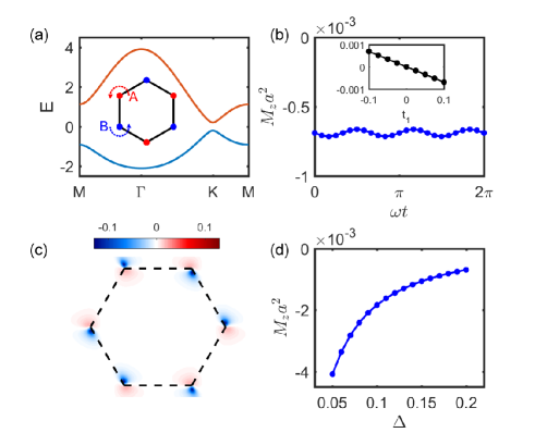
Figure 1: Model illustration of the orbital magnetization of Bloch electrons induced by the microscopic local rotation of atoms. (a) Band structure of a spinless-graphene toy model with first and second nearest neighbor hoppings. (b) Time dependence of the adiabatically induced magnetic moment in units of $e\omega a^{2}$ per unit cell. Here $\omega$ is the angular frequency of the atomic rotation, $a$ is the lattice constant, and we take the parameters as $\Delta=0.2t_{0}$, $t_{1}=0.1t_{0}$ and $\delta t_{0}=0.1t_{0}$. The insert shows that the pumped orbital magnetization in one period of the local rotations of atoms is proportional to the next nearest neighbor hopping parameter. (c) $\bm{k}$-space distribution of $\partial_{\bm{B}}a^{t}$ of the valence band. (d) Gap dependence of the pumped orbital magnetization.

Such a minimal model can thus be chosen as a spinless graphene-type one based on the honeycomb lattice taking into account the next nearest neighbor hopping, which is described by the Hamiltonian

$$\hat{H}(\bm{k})=t_{0}(F_{\mathrm{R}}\sigma_{x}-F_{\mathrm{Im}}\sigma_{y})+\Delta\sigma_{z}+t_{1}F_{\mathrm{NN}}\sigma_{0},$$ (25)

where $F_{\mathrm{R}}=2\cos x\cos y+\cos 2y$, $F_{\mathrm{Im}}=2\cos x\sin y-\sin 2y$, and $F_{\mathrm{NN}}=2\cos(2x/\sqrt{3})+4\cos(x/\sqrt{3})\cos\sqrt{3}y+3$ with $x=k_{x}a_{0}\sqrt{3}/2$, $y=k_{y}a_{0}/2$ and $a_{0}$ being the inter-atomic distance. The first and second nearest neighbor hoppings are $t_{0}$ and $t_{1}$, respectively, and a nonzero $t_{1}$ breaks the particle-hole symmetry. The staggered sublattice potential strength is $\Delta$.

Next, we add an adiabatic perturbation term due to the microscopic local rotation of atoms, and mainly follow the treatment introduced in Ref. Murakami2020 , where a right handed circularly polarized optical phonon mode at $\Gamma$ point is considered, with frequency $\omega$ and displacement vectors

$$\bm{u}_{A}=u_{0}(\cos\omega t,\sin\omega t),\text{ \ }\bm{u}_{B}=-\bm{u}_{A}$$ (26)

of A and B atoms on the two sublattices. There is a phase difference $\pi$ between the circular rotations of atoms A and B (see also Fig 1(a)), thus the nearest neighbor bond lengths change with time by the microscopic local rotations, while the next nearest neighbor ones do not. One can hence take these rotations as the modulation of the nearest neighbor hopping. By writing down the tight-binding Hamiltonian and converting it to a $\bm{k}$-space one, the resultant adiabatic perturbation to $\hat{H}(\bm{k})$ reads

$$\delta\hat{H}(\bm{k},t)= -\delta t_{0}(\sigma_{x}\sin y+\sigma_{y}\cos y)\sqrt{3}\sin x\cos\omega t$$

$$+ \delta t_{0}[(\cos x\cos y-\cos 2y)\sigma_{x}$$

$$-(\cos x\sin y+\sin 2y)\sigma_{y}]\sin\omega t,$$ (27)

where $\delta t_{0}\propto 2u_{0}$ arises from the change of the first nearest neighbor hopping energy due to the variation of the inter-atomic distance by the local rotations Murakami2020 . In our calculation, we consider the chemical potential inside the band gap and set $t_{0}$ as the energy unit, $t_{1}=0.1t_{0}$, and $\delta t_{0}=0.1t_{0}$.

With $\Delta=0.2t_{0}$, we plot energy bands in the absence of phonons in Fig. 1(a) where a band gap opens and the energy bands do not show particle-hole symmetry. In the presence of phonons, the adiabatic evolution of the electronic states due to the local rotations of A and B atoms leads to a time-dependent orbital magnetic moment, which is plotted in Fig. 1(b) in units of $\frac{et_{0}}{\hbar}a^{2}\frac{\hbar\omega}{t_{0}}$ (magnetic moment upon an area of $a^{2}$) in an evolution period. It is apparent that the induced orbital magnetization is proportional to the phonon frequency $\omega$. By using the parameters of graphene with $t_{0}=3$ eV and the lattice constant $a=\sqrt{3}a_{0}=2.46$ Å, $\frac{et_{0}}{\hbar}a^{2}$ is about 4.77$\mu_{B}$ with $\mu_{B}$ as the Bohr magneton. One can find a weak oscillation with a nonzero net contribution (about $-3.5\times 10^{-3}$ $\mu_{B}\frac{\hbar\omega}{t_{0}}$) upon one period of the local rotations of atoms, which implies a nonzero pumping of orbital magnetization. The $\bm{k}$-resolved instantaneous orbital magnetization $\partial_{\bm{B}}a^{t}$ is plotted in Fig. 1(c) where one can find that the main contribution is from K and K’ points with minimal interband spacings. As the band gap decreases, the magnitude of the induced magnetization increases rapidly (Fig. 1(d)).

We verify that the induced orbital magnetization vanishes with the next nearest neighbor hopping parameter $t_{1}$ in the insert in Fig. 1(b), which also shows that the pumped magnetization is proportional to $t_{1}$ at least up to $t_{1}=0.1t_{0}$. The resultant orbital magnetization pumping in the above toy model is of the same order as the pumped spin magnetization in a honeycomb lattice with very strong Rashba spin-orbit coupling (the Rashba coefficient equals to $0.4t_{0}$) Murakami2020 . We also mention that, in this latter four-band model, breaking the particle-hole symmetry is not required for supporting nonzero orbital magnetization pumped by rotations of atoms, and the pumped orbital and spin magnetization are also generally comparable (not shown here). Furthermore, taking $\hbar\omega/t_{0}=0.1$ (the ratio of the typical energy scales of phonons and electrons), the magnetic-moment pumping due to the periodic adiabatic change of electronic states induced by microscopic rotations of atoms is of the order of the nuclear magneton.

V.2 Intrinsic nonlinear anomalous Ettingshausen effect in 2D metals

Not only the electric current but also a thermal current carried by Bloch electrons can be induced by an applied electric field. In the intrinsic linear thermal current response to the electric field, the zero-field orbital magnetization plays a vital role Cooper1997 ; Xiao2006 ; Xiao2020EM . It is therefore anticipated that the electric-field induced orbital magnetization is indispensable in the second-order nonlinear intrinsic thermal current response to the electric field, i.e., the nonlinear intrinsic anomalous Ettingshausen effect. In this subsection we discuss in more detail the semiclassical picture of the electric-field induced orbital magnetization in 2D metals, and point out its key role in the intrinsic nonlinear anomalous Ettingshausen effect.

First, the electric-field modified orbital magnetization can be recast into an instructive form

$$\bm{M}=\int(f^{0}\bm{\tilde{m}}+eg^{0}\bm{\tilde{\Omega}})$$ (28)

in analogy to the magnetization (10) in the absence of electric fields. Here $\bm{\tilde{\Omega}}=\partial_{\bm{k}}\times[\bm{\mathcal{A}}^{k}+(\bm{a}^{k})^{\bm{E}}]$ is the electric-field modified Berry curvature, and

$$\bm{\tilde{m}}=\bm{m}+\partial_{\bm{B}}(e\bm{E}\cdot\bm{a}^{k})+e\bm{v}^{0}\times(\bm{a}^{k})^{\bm{E}}$$ (29)

is the orbital moment $\bm{\tilde{m}}=\frac{e}{2}\langle W|\left(\bm{\hat{r}}-\bm{r}_{c}\right)\times\bm{\hat{v}}|W\rangle$ up to the first order of the electric field. $\bm{m}$ is the zero-field orbital moment, $\bm{v}^{0}$ is the band velocity, and $(\bm{a}^{k})^{\bm{E}}$ is the positional shift linear in the electric field Gao2014 .

Second, a coarse graining process based on the wave-packet description of Bloch electrons Xiao2006 shows that, the electric-field induced local energy current density up to the second order is given by

$$\bm{j}^{\text{E}}=-e\bm{E}\times\int f^{0}\varepsilon\bm{\tilde{\Omega}}-\bm{E}\times\int f^{0}\bm{\tilde{m}}.$$ (30)

A magnetization current $\bm{j}^{\text{E,mag}}$ should be discounted to obtain the transport energy current density Cooper1997 $\bm{j}^{\text{E,tr}}=\bm{j}^{\text{E}}-\bm{j}^{\text{E,mag}}$. In uniform crystals, the energy magnetization current at the linear order of the electric field is given by the the material-dependent part of the Poynting vector describing the energy flow Xiao2006 : $\bm{j}^{\text{E,mag}}=-\bm{E}\times\bm{M}^{0}$. In the present nonlinear response, one has

$$\bm{j}^{\text{E,mag}}=-\bm{E}\times\bm{M}.$$ (31)

Consequently, the transport thermal current is given by

$$\bm{j}^{\text{h,tr}}=\bm{j}^{\text{E,tr}}-\frac{\mu}{e}\bm{j}=-e\bm{E}\times T\int s\left(\varepsilon\right)\bm{\tilde{\Omega}},$$ (32)

where $s\left(\varepsilon\right)=\left[\left(\varepsilon-\mu\right)f^{0}-g^{0}\right]/T$ is the entropy density contributed by a particular Bloch state, $\mu$ is the chemical potential, $T$ is the temperature, and we have made use of the result for the intrinsic nonlinear Hall electric current Gao2014 $\bm{j}=-e^{2}\bm{E}\times\int f^{0}\bm{\tilde{\Omega}}$.

By integration by parts, the entropy density takes the form of $s\left(\varepsilon\right)=\int d\eta\left(\eta-\mu\right)\partial_{\mu}f\left(\eta\right)\theta\left(\eta-\varepsilon\right)/T$, which renders the thermal transport current to be

$$\frac{\bm{j}^{\text{h,tr}}}{T}=-\frac{1}{e}\int d\eta\frac{\eta-\mu}{T}\frac{\partial f\left(\eta\right)}{\partial\eta}\bm{j}\left(\eta\right).$$ (33)

Here $\bm{j}\left(\eta\right)=-e^{2}\bm{E}\times\int\theta\left(\eta-\varepsilon\right)\bm{\tilde{\Omega}}$ is the nonlinear Hall electric current at zero temperature with Fermi energy $\eta$. This equation is completely parallel to the generalized Mott relation between the transport thermal current and electric current in the linear order of electric fields. At low temperatures much less than the distances between the chemical potential and band edges, the Sommerfeld expansion is legitimate Xiao2016 , hence the entropy density reduces to $s\left(\varepsilon\right)=\frac{1}{3}\pi^{2}k_{B}^{2}T\delta\left(\mu-\varepsilon\right)$, which is concentrated on the Fermi surface and decays dramatically away from it. Then the standard form of the Mott relation follows

$$\bm{j}^{\text{h}}/T=(\pi^{2}k_{B}^{2}T/3e)[\partial\bm{j}\left(\varepsilon\right)/\partial\varepsilon]|_{\varepsilon=\mu}.$$ (34)

Therefore, we extend the regime of validity of the Mott relation to the second-order intrinsic thermoelectric current responses to a constant electric field.

VI Summary

We have formulated a semiclassical theory for the orbital magnetization induced by general adiabatic evolutions of Bloch electronic states. This theory starts from formulating the electric current density in bulk, from which the magnetization can be extracted. The induced orbital magnetization is gauge dependent in general case but is gauge invariant only when the adiabatic time dependence is implicit or averaged out. These two cases correspond to the orbital magnetoelectric response and the periodic-evolution pumped orbital magnetization.

In the orbital magnetoelectric effect the adiabatic evolution is driven by a constant electric field, and the time dependence is only implicit through the evolution of mechanical crystal momentum. Thus the pertinent second Chern form current vanishes in 2D, making the 2D orbital magnetoelectricity governed completely by the perturbative term of the reciprocal-space Berry connection (Eqs. (16) and (17)), irrespective of insulators or metals. The role of the orbital magnetoelectricity in the nonlinear intrinsic anomalous Ettingshausen effect, which is proposed here as a transverse thermal current response in the second order of the driving electric field, has also been revealed in 2D metals. On the other hand, the orbital magnetoelectricity and the nonlinear intrinsic anomalous Ettingshausen effect in 3D metals are beyond the scope of the present theory. They may not be determined solely by bulk considerations and are left for future efforts.

In the context of the orbital magnetization pumped by periodic adiabatic evolutions in non-Chern insulators, the Chern-Simons contribution deduced from the second Chern form current can be present even in 2D. Meanwhile, as a second Chern form can be nonzero only if the system has more than two bands Xiao2009 , in a two-band minimal model the pumped magnetization is dictated solely by the perturbative term of the time component of the Berry connection [Eqs. (24) and (11)]. We illustrated the orbital magnetization pumping due to the periodic adiabatic change of electronic states induced by microscopic rotations of atoms in toy models based on the honeycomb lattice. The induced magnetization is of the same order as the pumped spin magnetization via strong Rashba spin orbit coupling.

The presented formulation is based on the assumption of well separated nondegenerate Bloch bands, whereas to explore the semiclassical theories in the case of degenerate bands and of closely located bands with possible non-adiabatic effects Tu2020 ; Woods2020 need separate studies.

Appendix A Derivation of gradient corrected wave-packet state

Given that the perturbative $\hat{H}^{\prime}$ is the form of the gradient correction, the first-order wave-packet reads

$$|W_{n}(\bm{k})\rangle =\sum_{\bm{p}}C_{n\bm{p}}\left[|\psi_{n\bm{p}}\rangle\right.$$

$$\left.+\sum_{n_{1}\bm{p}_{1}\neq n\bm{p}}\frac{\langle\psi_{n_{1}\bm{p}_{1}}|\hat{H}^{\prime}|\psi_{n\bm{p}}\rangle}{\varepsilon_{n\bm{p}}-\varepsilon_{n_{1}\bm{p}_{1}}}|\psi_{n_{1}\bm{p}_{1}}\rangle\right]$$

$$=\sum_{\bm{p}}e^{i\bm{p}\cdot\bm{\hat{r}}}[C_{n\bm{p}}|u_{n\bm{p}}\rangle+\sum_{n_{1}\neq n}C_{n_{1}\bm{p}}|u_{n_{1}\bm{p}}\rangle],$$ (35)

where

$$C_{n_{1}\bm{p}} =\sum_{\bm{p}_{1}}C_{n\bm{p}_{1}}\frac{\langle\psi_{n_{1}\bm{p}}|\hat{H}^{\prime}|\psi_{n\bm{p}_{1}}\rangle}{\varepsilon_{n\bm{p}_{1}}-\varepsilon_{n_{1}\bm{p}}}$$

$$=\sum_{n_{2}\bm{p}_{1}}C_{n\bm{p}_{1}}\frac{(\partial_{\bm{r}_{c}}\hat{H}_{c}\left(\bm{p}\right))_{n_{1}n_{2}}\cdot i(\bm{D}_{\bm{p}})_{n_{2}n}\delta_{\bm{pp}_{1}}}{\varepsilon_{n\bm{p}_{1}}-\varepsilon_{n_{1}\bm{p}}}$$

$$+\sum_{n_{2}\bm{p}_{1}}C_{n\bm{p}_{1}}\frac{(\partial_{\bm{r}_{c}}\hat{H}_{c}\left(\bm{p}_{1}\right))_{n_{2}n}\cdot i(\bm{D}_{\bm{p}})_{n_{1}n_{2}}\delta_{\bm{pp}_{1}}}{\varepsilon_{n\bm{p}_{1}}-\varepsilon_{n_{1}\bm{p}}}.$$ (36)

Here we introduced the notation

$$i(\bm{D}_{\bm{p}})_{n_{2}n}\equiv i\partial_{\bm{p}}\delta_{n_{2}n}+\bm{\mathcal{A}}_{n_{2}n}^{p}-\bm{r}_{c}\delta_{n_{2}n}.$$ (37)

After some manipulations we get Eq. (3) with

$$\Delta_{n_{1}n} =\frac{1}{2}(i\partial_{\bm{p}}+\bm{\mathcal{A}}_{n_{1}}^{p}-\bm{\mathcal{A}}_{n}^{p})\cdot(\partial_{\bm{r}_{c}}\hat{H}_{c})_{n_{1}n}$$

$$+\frac{1}{2}\sum_{n_{2}\neq n_{1}}\bm{\mathcal{A}}_{n_{1}n_{2}}^{p}\cdot(\partial_{\bm{r}_{c}}\hat{H}_{c})_{n_{2}n}$$

$$+\frac{1}{2}\sum_{n_{2}\neq n}(\partial_{\bm{r}_{c}}\hat{H}_{c})_{n_{1}n_{2}}\bm{\mathcal{A}}_{n_{2}n}^{p}-\bm{\mathcal{A}}_{n_{1}n}^{r_{c}}\cdot\bm{v}_{n}.$$ (38)

By using

$$\partial_{\bm{p}}\cdot(\partial_{\bm{r}_{c}}\hat{H}_{c})_{n_{1}n} =(\partial_{\bm{\hat{p}}}\cdot\partial_{\bm{r}_{c}}\hat{H}_{c})_{n_{1}n}$$

$$+i\sum_{n_{2}}[\bm{\mathcal{A}}_{n_{1}n_{2}}^{p}\cdot(\partial_{\bm{r}_{c}}\hat{H}_{c})_{n_{2}n}$$

$$-(\partial_{\bm{r}_{c}}\hat{H}_{c})_{n_{1}n_{2}}\cdot\bm{\mathcal{A}}_{n_{2}n}^{p}],$$ (39)

one gets Eq. (4). Here we also note that Eqs. (3) and (4) has also been obtained by a different method in a recent preprint Zhao2020 . In addition, when $[\partial_{\bm{r}_{c}}\hat{H}_{c},\bm{\hat{r}]}=0$, Eq. (4) reduces to $\Delta_{n_{1}n}\equiv\sum_{n_{2}\neq n}(\partial_{\bm{r}_{c}}\hat{H}_{c})_{n_{1}n_{2}}\cdot\bm{\mathcal{A}}_{n_{2}n}^{p}-\bm{\mathcal{A}}_{n_{1}n}^{r_{c}}\cdot\bm{v}_{n}$.

Appendix B Derivation of Eq. (8)

As shown in Ref. Dong2020 , one has

$$\int\left[d\bm{k}\right]d\bm{r}_{c}\mathcal{D}f\frac{\delta S}{\delta\bm{h}} =\int\mathcal{D}f[\frac{\partial L}{\partial\bm{h}}-\frac{d}{dt}\frac{\partial L}{\partial(\partial_{t}\bm{h})}]$$

$$-\partial_{r_{i}}\int\mathcal{D}f[\frac{\partial L}{\partial(\partial_{i}\bm{h})}-\frac{\partial L}{\partial(\partial_{t}\bm{h})}\dot{r}_{i}],$$ (40)

then the field variation formula (7) yields

$$\theta_{s}=\int\mathcal{D}f(\partial_{h_{s}}\tilde{\varepsilon}-\tilde{\Omega}_{s}^{h\mathcal{T}})-\partial_{r_{i}}\int f[d_{is}^{\theta}-\frac{\partial a^{t}}{\partial\left(\partial_{i}h_{s}\right)}].$$ (41)

Here $\tilde{\Omega}_{s}^{h\mathcal{T}}=\Omega_{si}^{hk}\dot{k}_{i}+\Omega_{si}^{hr}\dot{r}_{i}+\tilde{\Omega}_{s}^{ht}$, where $\dot{k}_{i}=-\partial_{i}\varepsilon+\Omega_{i}^{rt}$ and $\dot{r}_{i}=\partial_{k_{i}}\varepsilon-\Omega_{i}^{kt}$ up to the order of the product spatial and time derivatives according to the equations of motion, and only the Berry curvature $\Omega^{\bm{h}t}$ need be modified by inhomogeneity:

$$\tilde{\Omega}^{ht}=\partial_{\bm{h}}\mathcal{\tilde{A}}^{t}-\partial_{t}\bm{\mathcal{\tilde{A}}}^{h},\text{ \ }\bm{\mathcal{\tilde{A}}}^{h}=\frac{\partial\mathcal{\tilde{A}}^{t}}{\partial(\partial_{t}\bm{h})}=\bm{\mathcal{A}}^{h}+\bm{a}^{h}.$$ (42)

Then we arrive at

$$\theta_{s}\left(\bm{r},t\right) =\partial_{h_{s}}(G-\int f^{0}a^{t})-\partial_{r_{i}}[D_{is}^{\theta}-\int f^{0}\frac{\partial a^{t}}{\partial\left(\partial_{i}h_{s}\right)}]$$

$$-\int f^{0}(\Omega_{s}^{ht}+\Omega_{s}^{h\left[kr\right]t})+\partial_{t}\int f^{0}a_{s}^{h}$$

$$-\int\partial_{\varepsilon}f^{0}\delta\varepsilon\Omega_{s}^{ht}+\int(\partial_{h_{s}}f^{0}a^{t}-\partial_{t}f^{0}a_{s}^{h}),$$ (43)

where each term is gauge invariant, and the second Chern form of the Berry curvature is labeled as

$$\Omega_{si}^{hk}\Omega_{i}^{rt}+\Omega_{si}^{hr}\Omega_{i}^{tk}+\Omega_{s}^{ht}\Omega_{ii}^{kr}\equiv\Omega_{s}^{h\left[kr\right]t}.$$ (44)

Besides, $G=\int\mathcal{D}g\left(\tilde{\varepsilon}\right)$ is the electronic grand potential density and is evaluated to the first order of gradients, $g\left(\tilde{\varepsilon}\right)=g^{0}+f^{0}\delta\varepsilon$, and $\partial g\left(\tilde{\varepsilon}\right)/\partial\tilde{\varepsilon}=f\left(\tilde{\varepsilon}\right)=f^{0}+\partial_{\varepsilon}f^{0}\delta\varepsilon$, with $g^{0}=-\int_{\varepsilon}^{\infty}f(\eta)d\eta$ and $f^{0}=f\left(\varepsilon\right)$. $D_{is}^{\theta}=\int(f^{0}d_{is}^{\theta}+g^{0}\Omega_{is}^{kh})$ is the $\theta$-dipole density of the electron system, with $d_{ij}^{\theta}=\partial\delta\varepsilon_{n}/\partial\left(\partial_{i}h_{j}\right)$ being the $\theta$-dipole moment of a semiclassical Bloch electron Dong2020 .

In the case of $\bm{\hat{\theta}}=e\bm{\hat{v}}$ and $\bm{h}=-\bm{A}$, Eq. (43) reduces to Eq. (8).

On the other hand, in the absence of inhomogeneity Eq. (43) reduces to $\bm{\theta}\left(t\right)=\int f^{0}(\partial_{\bm{h}}\varepsilon-\bm{\Omega}^{\bm{h}t})$. In insulators, hence zero temperature for electrons, one has

$$\bm{\theta}\left(t\right)=\int\langle u|\bm{\hat{\theta}}\mathbf{|}u\rangle-\int\bm{\Omega}^{\bm{h}t}.$$ (45)

The first term on the right hand side is simply the average value of $\bm{\theta}$ in the electron system obtained by using the instantaneous Hamiltonian, whereas the second term is a geometric term related to the Berry curvature in $\left(t,\bm{h}\right)$ space

$$\bm{\Omega}^{\bm{h}t}=-\bm{\Omega}^{t\bm{h}}=2\operatorname{Re}\sum_{n_{1}\neq n}\frac{\mathcal{A}_{nn_{1}}^{t}\bm{\theta}_{n_{1}n}}{\varepsilon_{n}-\varepsilon_{n_{1}}}.$$ (46)

Equation (45) gives a unified account of diverse adiabatic responses of bounded operators in band insulators, such as the spin magnetoelectric effect, where the spin magnetization is induced by a weak electric field, and the spin magnetization pumped by microscopic local rotation of atoms Murakami2020 .

References

- (1) B. A. Bernevig, T. L. Hughes, and S.-C. Zhang, Phys. Rev. Lett. 95, 066601 (2005).
- (2) D. Go, J.-P. Hanke, P. M. Buhl, F. Freimuth, G. Bihlmayer, H.-W. Lee, Y. Mokrousov, and S. Blugel, Sci. Rep. 7, 46742 (2017).
- (3) S. Bhowal and S. Satpathy, Phys. Rev. B 101, 121112(R) (2020).
- (4) D. Xiao, J. Shi, and Q. Niu, Phys. Rev. Lett. 95, 137204 (2005).
- (5) T. Thonhauser, D. Ceresoli, D. Vanderbilt, and R. Resta, Phys. Rev. Lett. 95, 137205 (2005).
- (6) J. Shi, G. Vignale, D. Xiao, and Q. Niu, Phys. Rev. Lett. 99, 197202 (2007).
- (7) D. Ceresoli, U. Gerstmann, A. P. Seitsonen, and F. Mauri, Phys. Rev. B 81, 060409(R) (2010).
- (8) M. G. Lopez, D. Vanderbilt, T. Thonhauser, and I. Souza, Phys. Rev. B 85, 014435 (2012).
- (9) J.-P. Hanke, F. Freimuth, A. K. Nandy, H. Zhang, S. Blugel, and Y. Mokrousov, Phys. Rev. B 94, 121114(R) (2016).
- (10) V. M. Edelstein, Solid State Commun. 73, 233 (1990).
- (11) T. Yoda, T. Yokoyama, and S. Murakami, Sci. Rep. 5, 12024 (2015).
- (12) J. Lee, Z. Wang, H. Xie, K. F. Mak, and J. Shan, Nat. Mater. 16, 887 (2017).
- (13) C. Şahin, J. Rou, J. Ma, and D. A. Pesin, Phys. Rev. B 97, 205206 (2018).
- (14) L. Salemi, M. Berritta, A. K. Nandy, and P. M. Oppeneer, Nature Communications 10, 5381 (2019).
- (15) A. Johansson, B. Gobel, J. Henk, M. Bibes, and I. Mertig, arXiv: 2006.14958
- (16) I. Garate and A. H. MacDonald, Phys. Rev. B 80, 134403 (2009).
- (17) I. Garate and M. Franz, Phys. Rev. Lett. 104, 146802 (2010).
- (18) L. Dong, C. Xiao, B. Xiong, and Q. Niu, Phys. Rev. Lett. 124, 066601 (2020).
- (19) A. Malashevich, I. Souza, S. Coh, and D. Vanderbilt, New J. Phys. 12, 053032 (2010).
- (20) A. M. Essin, A. M. Turner, J. E. Moore, and D. Vanderbilt, Phys. Rev. B 81, 205104 (2010).
- (21) K.-T. Chen and P. A. Lee, Phys. Rev. B 84, 205137 (2011).
- (22) Y. Gao, S. A. Yang, and Q. Niu, Phys. Rev. Lett. 112, 166601 (2014).
- (23) L. Trifunovic, S. Ono, and H. Watanabe, Phys. Rev. B 100, 054408 (2019).
- (24) M. Hamada and S. Murakami, Phys. Rev. Res. 2, 023275 (2020).
- (25) L. Zhang and Q. Niu, Phys. Rev. Lett. 112, 085503 (2014).
- (26) D. A. Garanin and E. M. Chudnovsky, Phys. Rev. B 92, 024421 (2015).
- (27) G. Sundaram and Q. Niu, Phys. Rev. B 59, 14915 (1999).
- (28) D. Xiao, M.-C. Chang, and Q. Niu, Rev. Mod. Phys. 82, 1959 (2010).
- (29) Y. Gao, Frontiers of Physics 14, 33404 (2019).
- (30) N. R. Cooper, B. I. Halperin, and I. M. Ruzin, Phys. Rev. B 55, 2344 (1997).
- (31) C. Xiao and Q. Niu, Phys. Rev. B 101, 235430 (2020).
- (32) J.-H. Zhou, J. Hua, Q. Niu, and J.-R. Shi, Chin. Phys. Lett. 30, 027101 (2013).
- (33) D. Xiao, J. Shi, D. P. Clougherty, and Q. Niu, Phys. Rev. Lett. 102, 087602 (2009).
- (34) X.-L. Qi, T. L. Hughes, and S.-C. Zhang, Phys. Rev. B 78, 195424 (2008).
- (35) A. M. Essin, J. E. Moore, and D. Vanderbilt, Phys. Rev. Lett. 102, 146805 (2009).
- (36) J. M. Ziman, Principles of the Theory of Solids (Cambridge University Press, Cambridge, 1972).
- (37) D. Bulmash, P. Hosur, S.-C. Zhang, and X.-L. Qi, Phys. Rev. X 5, 021018 (2015).
- (38) T. Hayata and Y. Hidaka, Phys. Rev. B 95, 125137 (2017).
- (39) D. Varjas, A. G. Grushin, R. Ilan, and J. E. Moore, Phys. Rev. Lett. 117, 257601 (2016).
- (40) C. Xiao, H. Liu, J. Zhao, S. A. Yang, and Q. Niu, arXiv: 2002.01637
- (41) A. Gianfrate, O. Bleu, L. Dominici, V. Ardizzone, M. De Giorgi, D. Ballarini, G. Lerario, K. W. West, L. N. Pfeiffer, D. D. Solnyshkov, D. Sanvitto, and G. Malpuech, Nature 578, 381 (2020).
- (42) K.-T. Chen and P. A. Lee, Phys. Rev. B 86, 195111 (2012).
- (43) D. L. Bergman, Phys. Rev. Lett. 107, 176801 (2011).
- (44) M. Barkeshli and X.-L. Qi, Phys. Rev. Lett. 107, 206602 (2011).
- (45) L. L. Hirst, Rev. Mod. Phys. 69, 607 (1997).
- (46) P. T. Mahon and J. E. Sipe, Phys. Rev. Res. 2, 033126 (2020).
- (47) D. Xiao, Y. Yao, Z. Fang, and Q. Niu, Phys. Rev. Lett. 97, 026603 (2006).
- (48) C. Xiao, D. Li, and Z. Ma, Phys. Rev. B 93, 075150 (2016).
- (49) Matisse Wei-Yuan Tu, C. Li, H. Yu, and W. Yao, Phys. Rev. B 102, 045423 (2020).
- (50) T. Stedman and L. M. Woods, Phys. Rev. Res. 2, 033086 (2020).
- (51) Y. Zhao, Y. Gao, and D. Xiao, arXiv: 2009.09306