Trustworthy Online Marketplace Experimentation with Budget-split Design

Abstract

Online experimentation, also known as A/B testing, is the gold standard for measuring product impacts and making business decisions in the tech industry. The validity and utility of experiments, however, hinge on unbiasedness and sufficient power. In two-sided online marketplaces, both requirements are called into question. The Bernoulli randomized experiments are biased because treatment units interfere with control units through market competition and violates the “stable unit treatment value assumption”(SUTVA). The experimental power on at least one side of the market is often insufficient because of disparate sample sizes on the two sides. Despite the important of online marketplaces to the online economy and the crucial role experimentation plays in product improvement, there lacks an effective and practical solution to the bias and low power problems in marketplace experimentation. Our paper fills this gap by proposing an experimental design that is unbiased in any marketplace where buyers have a defined budget, which could be finite or infinite. We then provide generalizable system architecture for deploying this design to online marketplaces. Finally, we confirm our findings with empirical performance from experiments run in two real-world online marketplaces.

Keywords: A/B testing, controlled experiment, interference, online marketplaces

1 Introduction

Online experimentation (also known as A/B testing) has become the gold standard for measuring product impact and making business decisions in the tech industry. Companies such as Google, Facebook, Amazon, Microsoft and LinkedIn have all embraced this paradigm and built in-house platforms to enable large-scale online experimentation (Tang et al., 2010; Letham et al., 2019; Deng and Shi, 2016; Kohavi et al., 2012; Xu et al., 2015), commercial platforms have also emerged to provide online experimentation as a service to the broader audienceJohari et al. (2017). Because of the crucial role online experimentation plays in decision making and the scale at which it impacts the business, it is of utmost importance to ensure the unbiasedness and power of experiments. When an experiment is biased, the impact estimate is systematically incorrect and the quality of business decisions is compromised. This is especially detrimental if the bias is systematic. When the experiments do not have enough power, even large impacts are not statistically significant and are incorrectly neglected as ”neutral”, and when impacts do get detected, the throughput of experiments, therefore speed of innovation, is limited. These considerations are precisely why the majority of online experimentation literature is devoted to either designing unbiased experiments under an interference structure (Saveski et al., 2017; Eckles et al., 2017), or to increasing the power of an unbiased experiment (Deng et al., 2013).

The optimal strategy for designing unbiased and powerful experiments is highly dependent on the underlying interference structure. The most studied example of interference in the tech industry is that of the online social network (Saveski et al., 2017; Eckles et al., 2017), where each unit is the same type of entity (for example, a member of a social network). Each unit can connect with other units and interact with her connections.

Another important interference structure in online platforms, yet received little coverage, is that of online marketplaces. Unlike in a social network, the marketplace population consists of at least two types of units, sellers who offer goods, services or attention and buyers who purchase them with some currency. Marketplaces are an important part of the online economy, and usually are the products responsible for revenue generation in a tech companies. Therefore, it is important for both tech companies and the health of the online economy that we are able to experiment in online marketplaces unbiasedly and with high power. Some examples of online marketplaces are ads marketplace, where advertisers purchase the attention of platform members in the form of ads impressions (McMahan et al., 2013; He et al., 2014); hiring marketplace, where employers purchase the attention of job seekers in the form of job postings; and education platforms, where buyers purchase courses from educators that offer them.

The interference and network structure in online marketplaces present experimentation challenges to both unbiasedness and power. Bernoulli randomized experiments on either the seller-side or buyer-side violate the “stable unit treatment value assumption”(SUTVA) (Rubin, 2005; Johari et al., 2020) and are biased. To illustrate why SUTVA is violated, we use seller-side Bernoulli randomized experiments as an example. When a treatment increases the competitiveness of sellers, unless all buyers still have enough budget reserve to purchase more, the increased attractiveness of treatment sellers translates to relatively less attractiveness of control sellers, and the control sales decreases as treatment sales increases. Such interference in marketplaces violates the SUTVA assumption, which states a unit’s potential outcome should depend only on the treatment it receives and not on treatments other units receive. Analogous argument explains why buyer-side Bernoulli randomized experiments also violate SUTVA and are biased. In the marketing sphere, this bias is termed the “cannibalization bias”, to highlight the fact that treatment sales is higher than control sales not because total sales grows, but because treatment sales “cannibalizes” on control sales. Making a decision based on Bernoulli randomized experiments when cannibalization is present results in systematic overestimation of treatment effects. In any real-world marketplace, there are always limits to buyers’ budgets and sellers’ inventory, therefore both seller-side and buyer-side Bernoulli randomized experiments are subject to the cannibalization bias.

Beyond the cannibalization bias, marketplace experimentation is also plagued with insufficient experimental power. This happens because the two sides of the market usually consist of different types of entities, and are drastically disparate in numbers. For example, in an Ads marketplace, where buyers are enterprise advertisers or agencies, and sellers are consumer users, the number of buyers (Lara O’Reilly, 2015) can be three orders of magnitude smaller than the number of sellers (WebsiteBuilder, 2020). Similarly, in a physical goods marketplace, where buyers are consumers and sellers are more likely to be small businesses, the number of buyers is 60 times larger than the number of sellers (Emily Dayton, 2019). This disparity in sample size naturally leads to disparity in experimental power, and the insufficient power will be further exacerbated if the side with smaller sample size also has longer tails in metric distributions. This power disparity, or relative insufficiency on one side of the marketplace is undesirable because the marketplace business is only sustainable if both sides continues to be optimized, and one side of the marketplace having significantly lower experimental power means the speed of innovation and optimization is throttled on this side.

Solutions to marketplace experimentation in existing literature roughly follow two approaches: the analysis approach which first models the interference structure and cannibalization bias, and then apply model-based adjustments to the biased Bernoulli randomized experiments (Johari et al., 2020; Blake and Coey, 2014); the design approach, which explore alternative designs that are unbiased under weak and verifiable assumptions on the marketplace (Bojinov and Shephard, 2019; Jason (Xiao) Wang, 2018; Basse et al., 2016a). The analysis approach typically requires first simplifying the marketplace to a parametric model, when the modeling assumptions themselves are often untestable. In fact, if the model could accurately capture the marketplace, experimentation is not necessary and treatment effects can be measured through simulations. Some design approaches (Bojinov and Shephard, 2019; Jason (Xiao) Wang, 2018) are successful in achieving low bias under reasonable assumption, but the low bias comes at the cost of even lower power. Our paper contributes to the marketplace experimentation literature by proposing the budget-split design which overcomes both the bias and power challenges. The unbiasedness of the budget-split design requires one easy-to-validate assumption only, which is the buyers have a continuous budget (the budget can be finite or infinite). It is up to 30 times more powerful than alternative designs when deployed in the real-world marketplaces. The implementation and deployment of this design does not require an overhaul of the existing online marketplace infrastructure or the experimentation platform. Rather, only incremental changes to modules of the infrastructure. We note that our design shares some similarities with the budget allocation design in Basse et al. (2016a). Although both designs split the “budgets” in some ways, they are fundamentally different: in Basse et al. (2016a), an indirect, artificial “budget” (quota) is given to each buyer while the budget-split design considers the direct, natural budget that the buyers define. We also notice a recent blogpost in Greg Novak and Spiegel (2020) that outlines an inventory-split counterpart of the budget-split design. Our formal analysis of the budget-split design can be directly applied to the inventory-split settings with little modification.

The impact of the budget-split design is significant. It has enabled marketplace experimentation free of cannibalization bias; boosted experimental power to detect treatment effects that previously would have been dominated by noise. As a result, marketplace innovation and optimizations are carried out with much higher confidence and velocity. In this paper, we use the ads marketplace as a running example to present the budget-split design. The methodology, system architecture and empirical results can be readily extend to any marketplace where the buyer has a well-defined budget, such as the hiring marketplace. The rest of the paper is organized as follows. In Section 2, the causal inference problem in marketplaces is formally defined using the potential outcome framework. Section 3 introduces the budget-split design contrasts it with alternative designs such as cluster-based randomization and alternating-day design. Section 4 highlights the key considerations in system architecture and deployment of the budget-split design to online marketplaces. The empirical results on unbiasedness and power of the budget-split design are reported in Section 5. Finally, Section 6 concludes the paper with discussions and future research.

2 Experimentation in online ads marketplace

Experiments in an online ads marketplace (OAM) falls into the family of bipartite experiments where experimentation takes place in a bipartite graph, linking two types of entities – the buyers and the sellers(Pouget-Abadie et al., 2019; Doudchenko et al., 2020). Sellers are consumer members who visit the website, offer their attention and create requests for ads impressions, while buyers are advertisers that fulfill these requests with ads impressions. Each member visit can result in multiple ads requests to “sell” (i.e., the webpage can have multiple slots to show ads impressions during one visit). Each advertiser can create multiple campaigns that serve difference purposes, have different budgets, and target different member segments. Without loss of generality, we set our experimental units on the two sides as members and campaigns. Our framework can be applied to units at other granularity levels though. For example, it is common to set member sessions as the seller side units (finer) and advertisers as the buyer side units (coarser).

Suppose the marketplace contains $N$ members and $M$ campaigns, denoted by $i\in[N]=\{1,2,\ldots,N\}$ and $\mathcal{C}_{j},j\in[M]=\{1,2,\ldots,M\}$, respectively. For the $j$-th campaign $\mathcal{C}_{j}$, let $B_{j}\geq 0$ be its budget and the member set $I_{j}\subset[N]$ be its target population. Let $\bm{B}=\{B_{1},B_{2},\ldots,B_{M}\}$ denote the budgets of all campaigns. We note that targeting is at the member level. Thus if a member is targeted by a campaign, all requests created by this member are targeted. In addition, the campaigns can have different strategy and behavior, such as the bidding strategy and the pacing strategy. We do not model these details and instead simply represent these nuisances with parameter $\bm{\Theta}_{j}$. With these notations, we write the entire OAM as $\mathcal{M}=\{(\mathcal{C}_{j},I_{j},B_{j},\bm{\Theta}_{j})^{M}_{j=1}\}$. Figure 1 gives an illustration of an OAM.

There are two types of experiments in an OAM classified by the side of the market where the new feature is to be launched. When this feature acts on the seller-side, for example changing the placement of ads from top of the page to right rail of the page, a member-level experiment (ME) or a seller-side experiment needs to be performed to test its effect where the randomization units are members. Similarly, when the feature acts on the buyer-side, such as adjusting the bid price of a campaign, we need to conduct a campaign-level experiment (CE) or a buyer-side experiment where the randomization units are campaigns.

In this paper, we use ME to introduce the ideas. The budget-split design we propose also applies to CE. To simplify the demonstration, we defer the discussion of CE to Section 3.1 and focus on ME for now. In an ME, let $W_{i}\in\{0,1\}$ be the treatment received by member $i$, $\bm{W}=(W_{1},\ldots,W_{N})$ the treatment assignment vector of all members. Classical designs, such as the completely randomized design, can be directly applied to the seller side:

Definition 1 (Member-level completely randomized design).

A member-level completely randomized design is a probability distribution $\eta$ on $\{0,1\}^{N}$ such that for some $1\leq N_{1}\leq N$, $\eta(\bm{W})=1$ if $\sum^{N}_{i=1}W_{i}=N_{1}$ and $\eta(\bm{W})=0$ otherwise.

Unfortunately, as we show in Section 2.2 and Section 5.2, applying this design in OAM without modification and ignoring the buyer side can severely bias the treatment estimation. Similar bias is entailed when applying classical designs on the buyer side and ignoring the seller side.

Figure 1: An illustration of the online ads marketplace. The size of each campaign block represents its budget.

2.1 Potential outcomes and causal estimands

We adopt the potential outcomes framework (Rubin, 1974) for causal inference. For each $i\in[N]$ and $j\in[M]$, let $Y_{ij}(\bm{W};\bm{B})$ be the scalar potential outcome of member $i$ and campaign $\mathcal{C}_{j}$ given the treatment assignment vector and the budgets. Note that the potential outcomes are specified for each $(member,campaign)$ pair, which is the finest level in our design. A similar setup is also considered in Basse et al. (2016b). This general setup allows outcomes measured at coarser levels to be written as aggregations. For example, for situations in Doudchenko et al. (2020) and Pouget-Abadie et al. (2019) where the potential outcomes are specified in terms of only one side of the market, they can be defined by summing over indexes in $Y_{ij}(\bm{W};\bm{B})$ of the other side. Let $\bm{W}_{-i}$ be the $(N-1)$ vector by removing the $i$-th element from $\bm{W}$, we also consider an alternative parametrization of the potential outcomes as suggested by Chin (2018): $Y_{ij}(\bm{W};\bm{B})=Y_{ij}(W_{i},\bm{W}_{-i};\bm{B})$.

We focus on two metrics of special interests in an OAM: the value delivered to an advertiser and the revenue received by the marketplace operator. Specifically, let $Y_{ij}(\bm{W};\bm{B})\geq 0$ be the value delivered to campaign $\mathcal{C}_{j}$ (in fact, to the underlying advertiser) by the ads requests created by member $i$. If $i\not\in I_{j}$, member $i$ is not in the target population of $\mathcal{C}_{j}$ and $Y_{ij}(\bm{W};\bm{B})=0$ by definition. If $i\in I_{j}$, $\mathcal{C}_{j}$ competes for the ads slots from member $i$’s visits with all other campaigns $\mathcal{C}_{j^{\prime}}$ such that $i\in I_{j^{\prime}}$ by participating in an auction, such as the firce price auction or the generalized second price auction (Edelman et al., 2007). Note that the potential outcomes depend on the campaign budgets. In an OAM, $\mathcal{C}_{j}$’s own budget $B_{j}$ is used by the system to guide its pacing and bidding strategy (Agarwal et al., 2014), affecting its own bid underlying each $Y_{ij}$. At the same time, the resulting $Y_{ij}$ also depends on bids from other campaigns, which are themselves determined by their own budgets and actual spending. Unlike in (Basse et al., 2016b), we directly focus on the outcomes of the auction, ignoring the underlying bids as well as the auction mechanism for generality.

Aside from the value delivered to the advertisers, another crucial metric is the corresponding revenue received by the marketplace operator, denoted as $Y^{*}_{ij}(\bm{W};\bm{B})$. It is worth noting that $Y^{*}_{ij}(\bm{W};\bm{B})$ may or may not equal $Y_{ij}(\bm{W};\bm{B})$. Due to the complex optimization procedure under the hood, $Y_{ij}$ depends on $\bm{B}$ in a “not exact” manner, meaning that it is possible for $\sum_{i\in I_{j}}Y_{ij}(\bm{W};\bm{B})>B_{j}$, a phenomenon referred to as “over-delivery”. On the other hand, the platform cannot charge a campaign more than its budget. Therefore, we have for each $j$,

$$0\leq Y^{*}_{ij}(\bm{W};\bm{B}) \leq Y_{ij}(\bm{W};\bm{B})$$ (2.1)

$$\sum\limits_{i\in I_{j}}Y^{*}_{ij}(\bm{W};\bm{B}) \leq B_{j}.$$

In this work, we conduct inference conditioning on the potential outcomes and take treatment assignment as the only source of randomness. This randomization based inference strategy has the advantage of not entailing any modeling assumptions on $Y_{ij}(\bm{W};\bm{B})$. Due to the complex and evolving ecosystem in an OAM, modeling these potential outcomes can be extremely challenging.

We would like to estimate the treatment effect in terms of the total delivered value and the total received revenue conditioning on the budgets:

$$\tau(\bm{B}) =\sum\limits_{j\in[M]}\sum\limits_{i\in I_{j}}[Y_{ij}(\bm{1};\bm{B})-Y_{ij}(\bm{0};\bm{B})]=\sum\limits_{j\in[M]}\tau_{j}(\bm{B})$$ (2.2)

$$\tau^{*}(\bm{B}) =\sum\limits_{j\in[M]}\sum\limits_{i\in I_{j}}[Y^{*}_{ij}(\bm{1};\bm{B})-Y^{*}_{ij}(\bm{0};\bm{B})]=\sum\limits_{j\in[M]}\tau^{*}_{j}(\bm{B}),$$

where $\bm{1}=(1,1,\ldots,1)_{N}$ and $\bm{0}=(0,0,\ldots,0)_{N}$ denote the all treatment and all control treatment assignment.

The validity of vanilla A/B testing hinges critically on the stable unit treatment value assumption (SUTVA) (Imbens and Rubin, 2015), which states that (i) there is only a single form of each treatment variant and (ii) a unit’s potential outcome is unaffected by the treatment assignment of other units. The no interference assumption, however, is usually violated in marketplace experiments due to the limited campaign budgets. One special scenario where SUTVA at can be justified is in an imaginary world without budget constraints, so that the campaigns are free to bid on any of their targeted members based on their own evaluation of that member’s value. This is essentially the SUTVA for bids assumption made by Basse et al. (2016b). Formally, we have

Assumption 1 (No interference under unlimited budget).

If $B_{j}=\infty$ for each $j\in[M]$, we have $Y_{ij}(\bm{W};\bm{\infty})=Y_{ij}(W_{i};\bm{\infty})$.

In this case, the following simple plug-in estimator is unbiased:

$$\hat{\tau}_{j}(\bm{\infty}) =\sum\limits_{i\in I_{j}}\frac{W_{i}\cdot Y_{ij}(\bm{W};\bm{\infty})}{N_{1}/N}-\sum\limits_{i\in I_{j}}\frac{(1-W_{i})\cdot Y_{ij}(\bm{W};\bm{\infty})}{N_{0}/N},$$ (2.3)

where $N_{1}=\sum^{N}_{i=1}w_{i}$, $N_{0}=N-N_{1}$. Moreover, since there is no budget constraint, $Y_{ij}^{*}(\bm{W})=Y_{ij}(\bm{W})=Y_{ij}(W_{i})$ and the corresponding plug-in estimator $\hat{\tau}_{j}^{*}(\bm{\infty})$ for $\tau_{j}^{*}(\bm{\infty})$ is also unbiased.

2.2 Finite budget and the cannibalization bias

In reality, it is very unlikely that ads campaigns have unlimited budgets. As a result, Assumption 1 no longer holds and the potential outcomes are affected. With a finite budget, each campaign now needs to take a more “global” view over all its target members when planning its bid such that the total budget is split to different members wisely. For example, if the treatment has an edge over the control, a wise campaign should take this advantage and allocate more budget to members in the treatment group, resulting in interference between the potential outcomes. Due to this interference, the naive estimator for $\tau_{j}(\bm{B})$ and $\tau^{*}_{j}(\bm{B})$ as in (2.3) is no longer unbiased. To further illustrate this, we consider two examples. The first example illustrate that the naive estimator $\hat{\tau}_{j}^{*}(\bm{B})$ of $\tau_{j}^{*}(\bm{B})$ is biased in a very common scenario that can happen in a real OAM due to the strict budget constraints. The second example considers a more fundamental case, where even $\hat{\tau}_{j}(\bm{B})$ is biased. From now on, we assume that $0<B_{j}<\infty$ for campaign $j\in[M]$.

Example 1 (Full budget utilization).

Imagine an OAM that has a single buyer with a $100 budget, willing to purchase the sellers attention at $20 per impression; and many sellers each with a different propensity to pay attention to the buyers ads. Naturally, to better serve both the buyer’s and sellers’ interest, the marketplace improves the algorithm for matching the buyer with sellers who are most interested paying attention to the buyers ads. If the buyer already manages to spend the $100 budget under sub par seller ranking ($\sum_{i\in[N]}Y_{i1}^{*}(\bm{0};100)=100$), then improving seller ranking cannot further increase the buyer spending because there simply is no untapped budget (by definition, $\sum_{i\in[N]}Y_{i1}^{*}(\bm{1};100)\leq 100$ and $\tau^{*}_{1}(100)\leq 0$). On the other hand, had we run a member-level completely randomized experiment, with sellers in treatment being ranked by a better algorithm, we would have observed a positive treatment effect of the improved algorithm from the plug-in estimator.

Example 2 (Universally beneficial treatment with diminishing returns).

For some campaign $j$ with $I_{j}=[N]$, suppose that

$$\hskip 8.5359ptY_{ij}(0,|\bm{W}_{-i}|=N-1;\bm{B})$$ (2.4)

$$<\cdots$$

$$<Y_{ij}(0,|\bm{W}_{-i}|=1;\bm{B})$$

$$<Y_{ij}(0,\bm{0};\bm{B})<Y_{ij}(1,\bm{1};\bm{B})$$

$$<Y_{ij}(1,|\bm{W}_{-i}|=N-2;\bm{B})$$

$$<\cdots$$

$$<Y_{ij}(1,|\bm{W}_{-i}|=0;\bm{B}),$$

for any $i\in[N]$, where for $0\leq K<N$, $Y_{ij}(W_{i},|\bm{W}_{-i}|=K;\bm{B})=\{Y_{ij}(W_{i},\bm{W}_{-i};\bm{B}):\sum_{i\in I_{j}}\bm{W}_{-i}=K\}$. Intuitively, in this scenario, the treatment increases the value of each member. However, members in the treatment group are more valuable when the size of the treatment group is smaller; members in the control group are less valuable when the size of the treatment group is larger. (Consider an analogy to a job market in a county. If a job applicant is the only college graduate, he/she would probably be paid very high; with more and more applicants holding a college degree, the value of such a degree diminishes while those only holding a high school degree can find it harder to even get a job.) In this case,

$$\hskip 15.6491pt\mathbbm{E}[\hat{\tau}_{j}(\bm{B})]-\tau_{j}(\bm{B})$$ (2.5)

$$=\left\{\mathbbm{E}\left[\sum\limits_{i=1}^{N}\frac{W_{i}\cdot Y_{ij}(1,|\bm{W}_{-1}|=N_{1}-1;\bm{B})}{N_{1}/N}\right]-\sum\limits_{i=1}^{N}Y_{ij}(1,\bm{1};\bm{B})\right\}$$

$$+\left\{\sum\limits_{i=1}^{N}Y_{ij}(0,\bm{0};\bm{B})-\mathbbm{E}\left[\sum\limits_{i=1}^{N}\frac{(1-W_{i})\cdot Y_{ij}(0,|\bm{W}_{-1}|=|N_{1}|-1;\bm{B})}{N_{0}/N}\right]\right\}.$$

By (2.4), the two terms on the RHS are all positive. Thus $\hat{\tau}_{j}(\bm{B})$ has a positive bias.

Note that in (2.5), $\sum_{i=1}^{N}Y_{ij}(1,\bm{1};\bm{B})$ is overestimated while $\sum_{i=1}^{N}Y_{ij}(0,\bm{0};\bm{B})$ is underestimated. We thus refer to the bias of this naive estimator as the cannibalization bias as the new version of the product appears to be having an edge over the old one in an experiment, not only because it drives extra values of members in treatment, but also because it “cannibalises” the members’ values in control.

2.3 Switchback design

One popular strategy to get rid of this cannibalization bias is to treat the entire OAM at different times as the experimental units and adopt the switchback design (Bojinov et al., 2020). Let $t=1,2,\ldots,T$ be $T$ ordered time points. The switchback design assigns random treatment to each $\mathcal{M}_{t}$. Thus for each fixed $t$, all units (members or campaigns depending on whether the experiment is ME or CE) are assigned to the control or the treatment simultaneously. Since only one treatment is active at any time, there is no cannibalization bias due to cross treatment group intervention.

In practice, applying a switchback design to an OAM can be challenging. Firstly, although the design prevents any cross treatment interventions at any time point, it allows interventions across time points, often referred to as a carryover effect (Bojinov et al., 2020). In an OAM, the level of the carryover effect depends on the features being tested as well as other factors in the ecosystem. In general, it is hard to understand these carryover effects and analysis the switchback experiment properly. Secondly, a switchback experiment can be highly inefficient when it takes sometime for the effect of the feature to become measurable. For example, some features target at improving the performance of a campaign over a week. In this case, the time gap between different assignments has to be at least a week and the overall experimental period can stretch over weeks or even months. Thirdly, there is a conflict between the validity and the efficiency of a switchback experiment. On the one hand, a switchback experiment needs to run long enough to collect enough samples; on the other hand, it implicitly assumes that the OAM does not change much during the experimentation period, which is likely to be unrealistic when this period is long.

3 Budget-split design

In this section, we introduce a novel design that removes the cannibalization bias in both the member-level experiment and the campaign-level experiment in an OAM while bypassing the challenges in the switchback design. Our key motivation is that the cannibalization bias comes from interactions between units in different treatment groups. If these interactions are blocked, the cannibalization bias will not exist. Similar to the idea in Ha-Thuc et al. (2020), our goal is to simulate the two “counterfactuals” of the ads marketplace—one under the control and another under the treatment—with a design, such that a causal relationship can be established by directly comparing these two simulated marketplaces. The success of our strategy depends on two factors: (i) how similar the two simulated marketplaces are before the treatment, and (ii) how similar these simulated marketplaces are to the original marketplace before the treatment. As we shall see, our design automatically ensures (i), that is, the two marketplaces have exactly the same campaigns, very similar members, and the same underlying mechanism (i.e., auction mechanism, bidding strategy, etc.) We state (ii) formally in Assumption 3.5 and validate this assumption with real examples in Section 5.2.

Without loss of generality, we assume $I_{j}=[N]$ for all $\mathcal{C}_{j},j\in[M]$ in this section. Recall that the original OAM is $\mathcal{M}=\{(\mathcal{C}_{j},I_{j},B_{j},\bm{\Theta}_{j})^{M}_{j=1}\}$. We create two independent marketplaces $\mathcal{M}^{(0)}$ and $\mathcal{M}^{(1)}$ out of $\mathcal{M}$ with the following steps:

1. perform a random split of the members into two buckets of size $N^{(0)}$ and $N^{(1)}=N-N^{(0)}$. Let $d_{i}\in\{0,1\}$ be the bucket indicator of member $i$ and $\bm{d}=(d_{1},d_{2},\ldots,d_{N})$;

2. split the budget of each campaign $j$ accordingly:

   $$B_{j}^{(0)}=\frac{N^{(0)}}{N}\cdot B_{j} ,\quad B_{j}^{(1)}=\frac{N^{(1)}}{N}\cdot B_{j};$$ (3.1)

3. create a campaign $\mathcal{C}_{j_{0}}$ with a budget $B_{j}^{(0)}$ and a target population $I_{j_{0}}=\{i:d_{i}=0\}$. Let this campaign inherit all features (summarized by $\bm{\Theta}_{j}$) from campaign $\mathcal{C}_{j}$. Similarly, create a campaign $\mathcal{C}_{j_{1}}$;

4. replace $\mathcal{M}$ with two independent marketplaces:

   $$\mathcal{M}^{(0)} =\{(\mathcal{C}_{j_{0}},I_{j_{0}},B^{(0)}_{j},\bm{\Theta}_{j})^{M}_{j_{0}=1}\}$$ (3.2)

   $$\mathcal{M}^{(1)} =\{(\mathcal{C}_{j_{1}},I_{j_{1}},B^{(1)}_{j},\bm{\Theta}_{j})^{M}_{j_{1}=1}\}.$$

Recall that the treatment effect of interests is

$$\tau_{j}(\bm{B})=\sum\limits^{N}_{i=1}[Y_{ij}(\bm{1};\bm{B})-Y_{ij}(\bm{0};\bm{B})].$$ (3.3)

Intuitively, under the budget split setup, we use one of the $\mathcal{M}^{(l)}$’s to estimate $\sum^{N}_{i=1}Y_{ij}(\bm{1};\bm{B})$, and use another to estimate $\sum^{N}_{i=1}Y_{ij}(\bm{0};\bm{B})$. To this end, let $\tilde{W}_{l}\in\{0,1\}$ be the treatment indicator of OAM $\mathcal{M}^{l}$, where $\tilde{W}_{1}\sim\text{Bernoulli}(p)$ and $\tilde{W}_{0}=1-\tilde{W}_{1}$. If $\tilde{W}_{l}=1$, we apply the treatment to members in bucket $l$; if $\tilde{W}_{l}=0$, these members will receive the control.

Let $\bm{B}^{(l)}=\{B_{1}^{(l)},B_{2}^{(l)},\ldots,B_{M}^{(l)}\}$ and $\bm{W}^{(l)}=\{W_{i}:i\in I_{j_{l}}\}$ for $l=0,1$. Similar to the definition of $Y_{ij}(\bm{W};\bm{B})$, we define the potential outcomes associated with campaign $\mathcal{C}_{j_{l}}$ as $Y_{ij}^{(l)}(\bm{W}^{(l)};\bm{B}^{(l)}\mid\bm{d})$ for $l=0,1$ and $i\in I_{j_{l}}$. Note that these potential outcomes also depend on $\bm{d}$. (When defining these potential outcomes, we are actually making a no interference assumption, which is formally stated in Assumption 2.) Given a split $\bm{d}$, we consider the following estimator:

$$\hat{\tau}_{j}^{BS}(\bm{B}) =\sum\limits_{l=0,1}\tilde{W}_{l}\sum\limits_{i=1}^{N}\frac{\mathbbm{1}(d_{i}=l)Y_{ij}^{(l)}(\bm{1}_{N^{(l)}};\bm{B}^{(l)}\mid\bm{d})}{N^{(l)}/N}$$ (3.4)

$$-\sum\limits_{l=0,1}(1-\tilde{W}_{l})\sum\limits_{i=1}^{N}\frac{\mathbbm{1}(d_{i}=l)Y_{ij}^{(l)}(\bm{0}_{N^{(l)}};\bm{B}^{(l)}\mid\bm{d})}{N^{(l)}/N}.$$

To study the properties of $\hat{\tau}_{j}^{BS}(\bm{B})$, we first introduce the following definition:

Definition 2 (proportionally restricted campaign).

For $j\in[M]$, we define a proportionally restricted version of $\mathcal{C}_{j}$ as $\mathcal{C}_{j}(K)$, for $1\leq K\leq N$, such that $\mathcal{C}_{j}(K)$ is only allowed to target at $K$ members completely at random with a budget of $\mathcal{B}_{j}(K)=KB_{j}/N$. Moreover, suppose that all campaigns are proportionally restricted in a coupled manner, that is, they are restricted to the same members. Then for each $i\in[N]$, we can define the potential outcomes associated with $\mathcal{C}(K)$ as $\mathcal{Y}_{ij}(\bm{W};\mathcal{B}(K)\mid\bm{d})$, where $\mathcal{B}(K)=\{\mathcal{B}_{1}(K),\ldots,\mathcal{B}_{M}(K)\}$, $\bm{d}=(d_{1},d_{2},\ldots,d_{N})$, $d_{i}$ the indicator of whether member $i$ is in the restricted target population. For convenience, we define $\mathcal{Y}_{ij}(\bm{W};\mathcal{B}(K)\mid\bm{d})=0$ if $d_{i}=0$.

In practice, this definition is relevant to the throttling procedure that can be applied before the auctions take place (Basse et al., 2016b). For example, due to resource constraint, the system could not afford to allow each campaign to bid for all its targeting members. We next state two assumptions on the potential outcomes of proportionally restricted campaigns. Assumption 2 limits the interference to members within the restricted target population. Assumption 3.5 ensures that the restricted campaigns are on average “similar enough” to the unrestricted ones such that they can be used to perform inference about the original campaigns.

Assumption 2 (Limited interference).

For each $i\in[N]$, $j\in[M]$ and $\bm{W}$, we assume $\mathcal{Y}_{ij}(\bm{W};\mathcal{B}(K)\mid\bm{d})=\mathcal{Y}_{ij}(\bm{W}_{\bm{d}=1};\mathcal{B}(K)\mid\bm{d})$, where $\bm{W}_{\bm{d}=1}$ represents the elements in $\bm{W}$ with $\bm{d}=1$.

Assumption 3 (Stable system).

For each $j$ and $1\leq K\leq N$, we assume

$$\frac{1}{N}\sum\limits^{N}_{i=1}Y_{ij}(\bm{1};\bm{B}) =\mathbbm{E}_{\bm{d}}\left[\frac{1}{K}\sum\limits_{i=1}^{N}d_{i}\mathcal{Y}_{ij}(\bm{1}_{K};\mathcal{B}(K)\mid\bm{d})\right]$$ (3.5)

$$\frac{1}{N}\sum\limits^{N}_{i=1}Y_{ij}(\bm{0};\bm{B}) =\mathbbm{E}_{\bm{d}}\left[\frac{1}{K}\sum\limits_{i=1}^{N}d_{i}\mathcal{Y}_{ij}(\bm{0}_{K};\mathcal{B}(K)\mid\bm{d})\right].$$

Assumption 3.5 characterizes a degree of stability of the system. It requires that a proportionally restricted campaign behaves in a similar manner to its original campaign so that the two created OAMs are similar to the original one. In practice, this assumption is more likely to hold when (i) $K$ is large and (ii) $N$ is large. When $K$ is close to $N$, the $\mathcal{C}_{j}(K)$ is essentially $\mathcal{C}_{j}$. When $K$ decreases, the ecosystem underlying $\mathcal{C}_{j}(K)$ becomes less similar to that of $\mathcal{C}_{j}$ and the reliability of this assumption decreases accordingly. In the extreme case when $K$ is close to $1$, $\mathcal{C}_{j}(K)$ essentially loses all its flexibility in participating in auctions. As a result, the potential outcomes of $\mathcal{C}_{j}(K)$ can be totally distorted from those of $\mathcal{C}_{j}$. In reality, there is usually some burn-in threshold $K_{0}$ such that the system (i.e., the bidding strategies of the campaigns) stabilizes with $K_{0}$ members. In this case, if $N$ is very large such that $K>K_{0}$, $\mathcal{C}_{j}(K)$ would behave very similarly to $\mathcal{C}_{j}$. Fortunately, in OAM, $N$ is usually at least at the scale of millions, in which case $K>K_{0}$ can be easily satisfied with $K=O(N)$. We note that $K_{0}$ depends on the level of homogeneity of members. $K_{0}$ of a market where the members are very similar to each other is generally smaller than $K_{0}$ in a more heterogeneous market.

Theorem 1.

Under Assumption 2 and Assumption 3.5, if in addition $N^{(0)}=N^{(1)}=N/2$, $p=0.5$, the budget split estimator in (3.4) is unbiased: for each $j\in[M]$,

$$\mathbbm{E}_{\tilde{W}_{1},\bm{d}}[\hat{\tau}_{j}^{BS}(\bm{B})]=\tau_{j}(\bm{B}).$$ (3.6)

The proof is standard and can be found in Appendix B.

3.1 Campaign-level experiments

So far, we have been focusing on ME. Since the budget split framework creates two complete OAM with both the buyer side and the seller side, it can also be used for CE. A CE is involved when the features to be tested act on the buyer-side. Examples of such features include UI changes at the campaign management portal and adjustments to the underlying campaign bidding strategy.

Similar to the setup in Section 2, let $W^{c}_{j}\in\{0,1\}$ be the treatment received by campaign $\mathcal{C}_{j}$, $j\in[M]$ and let $Y^{c}_{ij}(\bm{W}^{c};\bm{B})$ be the corresponding potential outcomes. Again, we consider the treatment effect in terms of the total delivered value:

$$\tau^{c}(\bm{B}) =\sum\limits_{j\in[M]}\sum\limits_{i\in I_{j}}[Y^{c}_{ij}(\bm{1}^{c};\bm{B})-Y^{c}_{ij}(\bm{0}^{c};\bm{B})]=\sum\limits_{j\in[M]}\tau^{c}_{j}(\bm{B}).$$ (3.7)

Under the budget split framework, the setup for CE is essentially the same as for ME. In this case, $\tau^{c}_{j}(\bm{B})$ is estimated directly by comparing the two campaigns $\mathcal{C}_{j_{0}}$ and $\mathcal{C}_{j_{1}}$ with an estimator similar to (3.4).

Although the same budget-split framework is used for both ME and CE, the resulting experiments have very different nature. In ME, the budget split design essentially performs a completely randomized experiment at the 50-50 split, where the treatment assignments coincide with the budget allocations. Here we adopt the budget split design to remove the cannibalization bias. In CE, the budget split design has a more direct motivation. Namely, we create two (approximately) identical replicates for each experimental units before the experiment and solve the “fundamental problem of causal inference” (Holland, 1986) by making the two potential outcomes of each unit directly observable. Instead of estimated or imputed, the potential outcomes are observed under the budget split design. Therefore, the causal estimands are also observed directly.

For CE, both the switchback design (SB) and the budget split design (BS) aim at creating “counterfactuals” of any experimental unit (campaign) and making the potential outcomes observable under both treatments. In SB, campaign $\mathcal{C}_{j}$ at different time points serve as its “counterfactuals”. In the BS, the “counterfactuals” are represented by the two half-sized campaigns $\mathcal{C}_{j_{0}}$ and $\mathcal{C}_{j_{1}}$ that are active simultaneously. When making causal comparisons, SB keeps the size of the campaigns unchanged while BS controls for the time factor.

4 System Architecture

Having presented the budget-split design and highlighted its advantages over member-level experiments, campaign-level experiments and switchback experiments, we now give guidelines for the system architecture changes for deploying this design onto the online ads marketplace. Note that the modules in the ads marketplace are also ubiquitous in other types of marketplaces such as hiring marketplaces and physical goods marketplaces.

To set the context, we introduce the important components in the infrastructure of an online ads marketplace:

1. At the core of an online ads marketplace, is an ad server that receives incoming ads requests and responds with ads impressions in real time. Within the ads server, a pacing/bidding module controls the spending speed of each campaign, and eventually when to stop serving impressions. The pacing/bidding module makes serving decisions based on auction signals such as bid price, targeting and auction participation rate.

2. The tracker service supports the ad server by keeping track of ads events such as impressions, clicks and tallying the campaign-level cumulative spending, along with other performance metrics, such as the click-through rate. Combined with the core ad server, it forms a feedback loop for ads serving, enabling the pacing/bidding module to be built as a feedback controller.

3. Finally, the marketplace interfaces with advertisers through the campaign management system, where advertiers create and manage their ads campaigns, as well as get billed and reported on campaign performance.

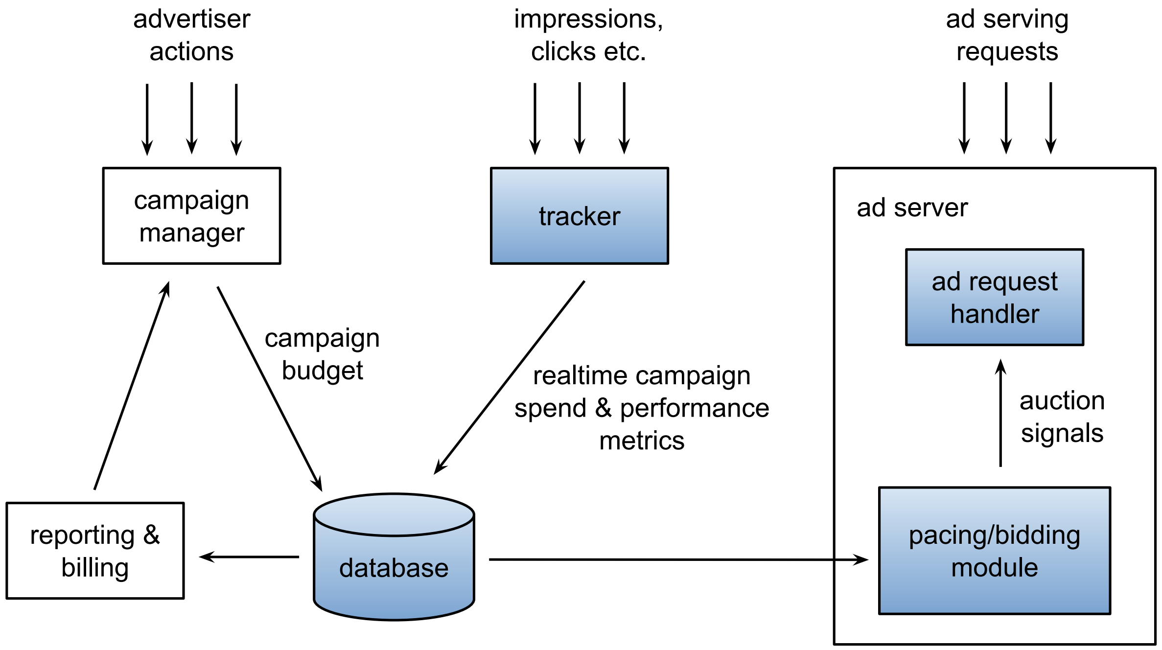
Figure 2: System architecture for the budget-split design.

To implement the budget-split design, the components marked as blue in figure 2 are modified, in the following ways:

1. In the request receiving and responding tier of the ad server, all requests from a member is randomized into either treatment or control depending on the member ID. This is the member-level randomization as described in Section 3.

2. In the tracker service, treatment assignment in step 1 together with ads campaign ID are recorded in the tracking information of the request.

3. In the pacing/bidding module of the ad server, all the originally campaign-level controller inputs are now replaced with their campaign-treatment-level counterparts. As an example, budget is now set at campaign-treatment-level as described in Section 3 rather than at campaign-level. Furthermore, feedback signals are provided at per-treatment level. Consequently, the pacing/bidding controller outputs auction signals at the campaign-treatment-level.

   Then, the real time auctions, along with any other serving decisions such as whether an ad should stop or resume serving, are carried out using the campaign-treatment-level signals in lieu of campaign-level ones.

With these changes in place, the feedback data and control paths for each treatment become entirely independent of other treatments, for each campaign and across all campaigns. Effectively every treatment now owns a standalone marketplace. This is exactly an implementation of the budget-split design as defined in Section 3.

5 Empirical Results

The budget-split experimentation has since been deployed to two online marketplaces. Similar to what was proven in Section 3, it was shown to be much more powerful than alternative designs such as campaign-level experiments or switchback experiments; and not susceptible to cannibalization bias as campaign-level and member-level experiments are.

5.1 Power Gain

In the two marketplaces where budget-split was deployed, we compared the power curves of budget-split experiments versus campaign-level and switchback experiments. Switchback experiments were analyzed with paired permutation tests to boost the power; all other designs are analyzed with two-sample t-tests.

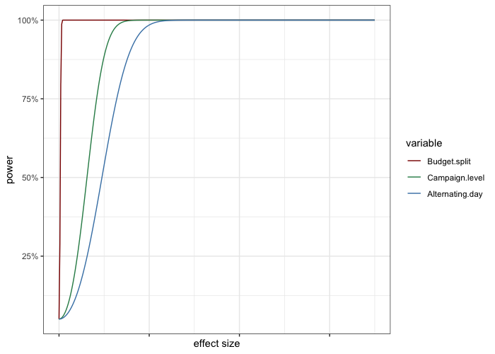
Figure 3: Power curves for marketplace 1

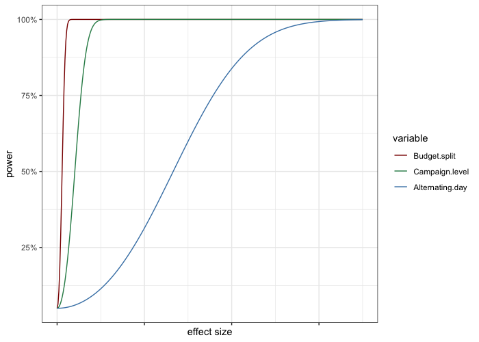
Figure 4: Power curves for marketplace 2

As shown in Figure 3 and Figure 4, for the effect size that budget-split has 80% power to detect, campaign-level experiments have power 5.2% (Marketplace 1) and 12% (Marketplace 2), while switchback experiments have only 5.1% (Marketplace 1) and 5.2% (Marketplace 2) power to detect the effect.

Even though switchback experiments are expected to be unbiased when no carry-over effect exists in the marketplace, they practically have such low power that detecting treatment effects becomes challenging. It is worth noting that 5% power is actually the lowest power possible for a 5% level test. Campaign-level experiments are not only biased, but also just barely more powerful than switchback experiments. In practice, budget-split experiments have enabled detection of negative product impacts on the order of millions of dollars (in terms of annual revenue) that previously went undetected in a campaign-level experiment because of insufficient power.

5.2 Robustness against Cannibalization Bias

As discussed in Section 3, the budget-split design effectively removes interference between treatment units and control units through splitting the campaign budgets, and is not susceptible to the cannibalization bias even in place of market competition. In comparison, switchback experiments are unbiased when no carry-over effect is present; cluster-based randomization is unbiased when there is no interference among clusters, which often is not practically feasibleSaveski et al. (2017); member-level and campaign-level experiments are biased because they do not account for the interference from market competition at all. In this section, we compare the impacts measured in budget-split design versus in member-level experiments to showcase the amount of cannibalization bias. It is worth noting that budget-split design was not compared against campaign-level experiments, switchback experiments or cluster-based experiments because these designs are too insufficiently powered for comparison.

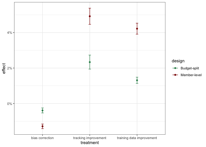
Figure 5: Measurement of Cannibalization Bias

The presence of cannibalization bias in marketplace experiment when interference are not accounted for is confirmed in Figure 5. The exact amount of bias depends on the nature of the treatment, but not accounting for interference typically results in one to two times overestimation of the treatment effect. We have not yet encountered a treatment where cannibalization bias changes the sign of the treatment effect, but this is not impossible if, for example, the treatment positively impacts budget-constraint campaigns and negatively impacts non budget-constraint campaigns.

6 Discussions

In this paper, we presented the budget-split design as the solution to cannibalization bias and insufficient power in marketplace experimentation. Rather than relying on modeling assumptions that are often impossible to validate, the budget-split design only requires one side of the marketplace having a defined and splittable budget, and no additional assumptions. We formulated the marketplace experimentation problem under the potential outcome framework, defined the estimand, derived an unbiased estimator for the estimand under budget-split design. We showed the bias and variance reduction nature of budget-split design relative to alternative designs with empirical results.

This work, however, is only the start of experimentation in online marketplaces. Future work is need to accurately compute the variance estimators under the budget-split design; extend the budget-split design to marketplaces where the budget is discrete; and increase throughput of budget-split experiments by enabling multiple simultaneous orthogonal budget-split experiments in the marketplace.

Supplementary Materials

A Illustration of the cannibalization bias

As a further illustration to the cannibalization bias, we consider a special case of Example 2 in Section 2.2. For simplicity, we take a super-population perspective and assume the potential outcomes are generated by the following model:

$$Y_{i1}(\bm{W};B_{1})=\mu+\tau W_{i}-\gamma\cdot\frac{e^{\frac{\sum^{N}_{j=1}W_{j}}{N}-1}-1/e}{1-1/e}+\epsilon_{i},$$ (S1)

where $\mu=5$, $\tau=2$, $\gamma=1$ and $\mathbbm{E}[\epsilon_{i}]=0$. In a completely randomized experiment with $N_{i}=pN$, Figure S6 shows the expected group means for the two treatment groups. In this example, we have a constant cannibalization bias $\gamma$, which equals $\Delta_{1}+\Delta_{2}$ in Figure S6. Note that when $\tau=0$, the real treatment effect is zero and we have an illustration of Example 1 in Section 2.2.

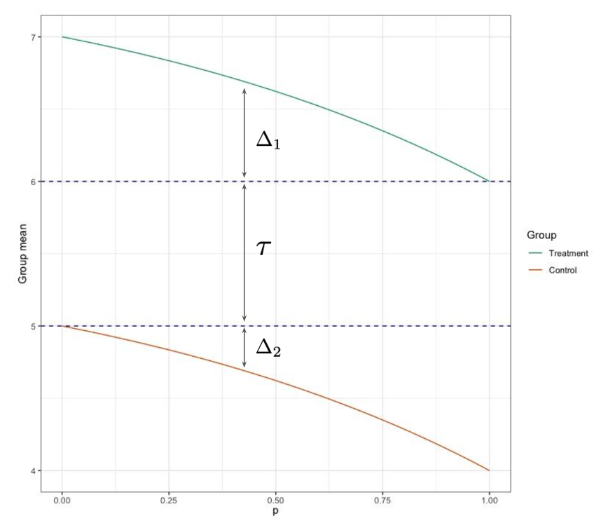
Figure S6: Example of the cannibalization bias

7 Proof of Theorem 1

Proof.

Under the budget-split design, the two sub-campaigns created out of campaign $j$ are essentially two proportionally restricted versions of $j$. Specifically, we have

$$Y_{ij}^{(l)}(\bm{1}_{N^{(l)}};\bm{B}^{(l)}\mid\bm{d}) =\begin{cases}&\mathcal{Y}_{ij}(\bm{1}_{N^{(1)}};\mathcal{B}(N^{(1)})\mid\bm{d}),\quad l=1,d_{i}=1\\ &\mathcal{Y}_{ij}(\bm{1}_{N^{(0)}};\mathcal{B}(N^{(0)})\mid 1-\bm{d}),\quad l=0,d_{i}=0\\ \end{cases}$$ (S1)

$$Y_{ij}^{(l)}(\bm{0}_{N^{(l)}};\bm{B}^{(l)}\mid\bm{d}) =\begin{cases}&\mathcal{Y}_{ij}(\bm{0}_{N^{(1)}};\mathcal{B}(N^{(1)})\mid\bm{d}),\quad l=1,d_{i}=1\\ &\mathcal{Y}_{ij}(\bm{0}_{N^{(0)}};\mathcal{B}(N^{(0)})\mid 1-\bm{d}),\quad l=0,d_{i}=0\\ \end{cases}.$$

Therefore,

$$\hskip 15.6491pt\mathbbm{E}_{\tilde{W}_{1},\bm{d}}\left[\sum\limits_{l=0,1}\tilde{W}_{l}\sum\limits_{i=1}^{N}\frac{\mathbbm{1}(d_{i}=l)Y_{ij}^{(l)}(\bm{1}_{N^{(l)}};\bm{B}^{(l)}\mid\bm{d})}{N^{(l)}/N}\right]$$ (S2)

$$=\mathbbm{E}_{\bm{d}}\left[\frac{1}{2}\sum\limits_{l=0,1}\sum\limits_{i=1}^{N}\frac{\mathbbm{1}(d_{i}=l)Y_{ij}^{(l)}(\bm{1}_{N^{(l)}};\bm{B}^{(l)}\mid\bm{d})}{1/2}\right]$$

$$=\mathbbm{E}_{\bm{d}}\Bigg{[}\sum\limits_{i=1}^{N}\mathbbm{1}(d_{i}=0)Y_{ij}^{(0)}(\bm{1}_{N^{(0)}};\bm{B}^{(0)}\mid\bm{d})$$

$$\hskip 25.6073pt+\sum\limits_{i=1}^{N}\mathbbm{1}(d_{i}=1)Y_{ij}^{(1)}(\bm{1}_{N^{(1)}};\bm{B}^{(1)}\mid\bm{d})\Bigg{]}$$

$$=\mathbbm{E}_{1-\bm{d}}\Bigg{[}\sum\limits_{i=1}^{N}\mathbbm{1}(1-d_{i}=1)\mathcal{Y}_{ij}(\bm{1}_{N^{(0)}};\mathcal{B}(N^{(0)})\mid 1-\bm{d})\Bigg{]}$$

$$\hskip 8.5359pt+\mathbbm{E}_{\bm{d}}\left[\sum\limits_{i=1}^{N}\mathbbm{1}(d_{i}=1)\mathcal{Y}_{ij}(\bm{1}_{N^{(1)}};\mathcal{B}(N^{(1)})\mid\bm{d})\right]$$

$$=\frac{1}{2}\sum\limits^{N}_{i=1}Y_{ij}(\bm{1};\bm{B})+\frac{1}{2}\sum\limits^{N}_{i=1}Y_{ij}(\bm{1};\bm{B})$$

$$=\sum\limits^{N}_{i=1}Y_{ij}(\bm{1};\bm{B}).$$

Similarly,

$$\hskip 15.6491pt\mathbbm{E}_{\tilde{W}_{1},\bm{d}}\left[\sum\limits_{l=0,1}(1-\tilde{W}_{l})\sum\limits_{i=1}^{N}\frac{\mathbbm{1}(d_{i}=l)Y_{ij}^{(l)}(\bm{0}_{N^{(l)}};\bm{B}^{(l)}\mid\bm{d})}{N^{(l)}/N}\right]$$ (S3)

$$=\sum\limits^{N}_{i=1}Y_{ij}(\bm{0};\bm{B}).$$

$\square$

References

- Agarwal et al. (2014) Agarwal, D., S. Ghosh, K. Wei, and S. You (2014). Budget pacing for targeted online advertisements at linkedin. In Proceedings of the 20th ACM SIGKDD international conference on Knowledge discovery and data mining, pp. 1613–1619.
- Basse et al. (2016a) Basse, G. W., H. A. Soufiani, and D. Lambert (2016a). Randomization and the pernicious effects of limited budgets on auction experiments. In A. Gretton and C. C. Robert (Eds.), Proceedings of the 19th International Conference on Artificial Intelligence and Statistics, AISTATS 2016, Cadiz, Spain, May 9-11, 2016, Volume 51 of JMLR Workshop and Conference Proceedings, pp. 1412–1420. JMLR.org.
- Basse et al. (2016b) Basse, G. W., H. A. Soufiani, and D. Lambert (2016b). Randomization and the pernicious effects of limited budgets on auction experiments. In Artificial Intelligence and Statistics, pp. 1412–1420.
- Blake and Coey (2014) Blake, T. and D. Coey (2014). Why marketplace experimentation is harder than it seems: The role of test-control interference. In Proceedings of the Fifteenth ACM Conference on Economics and Computation, EC ’14, New York, NY, USA, pp. 567–582. Association for Computing Machinery.
- Bojinov and Shephard (2019) Bojinov, I. and N. Shephard (2019). Time series experiments and causal estimands: Exact randomization tests and trading. Journal of the American Statistical Association 114(528), 1665–1682.
- Bojinov et al. (2020) Bojinov, I., D. Simchi-Levi, and J. Zhao (2020). Design and analysis of switchback experiments. Available at SSRN 3684168.
- Chin (2018) Chin, A. (2018). Central limit theorems via stein’s method for randomized experiments under interference. arXiv preprint arXiv:1804.03105.
- Deng and Shi (2016) Deng, A. and X. Shi (2016). Data-Driven Metric Development for Online Controlled Experiments. In Proceedings of the 22nd ACM SIGKDD International Conference on Knowledge Discovery and Data Mining - KDD ’16.
- Deng et al. (2013) Deng, A., Y. Xu, R. Kohavi, and T. Walker (2013). Improving the sensitivity of online controlled experiments by utilizing pre-experiment data. In Proceedings of the Sixth ACM International Conference on Web Search and Data Mining, WSDM ’13, New York, NY, USA, pp. 123–132. Association for Computing Machinery.
- Doudchenko et al. (2020) Doudchenko, N., M. Zhang, E. Drynkin, E. Airoldi, V. Mirrokni, and J. Pouget-Abadie (2020). Causal inference with bipartite designs. arXiv preprint arXiv:2010.02108.
- Eckles et al. (2017) Eckles, D., B. Karrer, and J. Ugander (01 Mar. 2017). Design and analysis of experiments in networks: Reducing bias from interference. Journal of Causal Inference 5(1), 20150021.
- Edelman et al. (2007) Edelman, B., M. Ostrovsky, and M. Schwarz (2007). Internet advertising and the generalized second-price auction: Selling billions of dollars worth of keywords. American economic review 97(1), 242–259.
- Emily Dayton (2019) Emily Dayton (2019). Amazon statistics you should know: Opportunities to make the most of america’s top online marketplace.
- Greg Novak and Spiegel (2020) Greg Novak, S. S. and D. Spiegel (2020). Experimentation with resource constraints.
- Ha-Thuc et al. (2020) Ha-Thuc, V., A. Dutta, R. Mao, M. Wood, and Y. Liu (2020). A counterfactual framework for seller-side a/b testing on marketplaces. In Proceedings of the 43rd International ACM SIGIR Conference on Research and Development in Information Retrieval, pp. 2288–2296.
- He et al. (2014) He, X., J. Pan, O. Jin, T. Xu, B. Liu, T. Xu, Y. Shi, A. Atallah, R. Herbrich, S. Bowers, and J. Q. n. Candela (2014). Practical lessons from predicting clicks on ads at facebook. In Proceedings of the Eighth International Workshop on Data Mining for Online Advertising, ADKDD’14, New York, NY, USA, pp. 1–9. Association for Computing Machinery.
- Holland (1986) Holland, P. W. (1986). Statistics and causal inference. Journal of the American statistical Association 81(396), 945–960.
- Imbens and Rubin (2015) Imbens, G. W. and D. B. Rubin (2015). Causal inference in statistics, social, and biomedical sciences. Cambridge University Press.
- Jason (Xiao) Wang (2018) Jason (Xiao) Wang (2018). The design of a/b tests in an online marketplace.
- Johari et al. (2017) Johari, R., P. Koomen, L. Pekelis, and D. Walsh (2017). Peeking at a/b tests: Why it matters, and what to do about it. In Proceedings of the 23rd ACM SIGKDD International Conference on Knowledge Discovery and Data Mining, KDD ’17, New York, NY, USA, pp. 1517–1525. Association for Computing Machinery.
- Johari et al. (2020) Johari, R., H. Li, and G. Y. Weintraub (2020). Experimental design in two-sided platforms: An analysis of bias. Proceedings of the 21st ACM Conference on Economics and Computation.
- Kohavi et al. (2012) Kohavi, R., A. Deng, B. Frasca, R. Longbotham, T. Walker, and Y. Xu (2012). Trustworthy Online Controlled Experiments : Five Puzzling Outcomes Explained. Proceedings of the 18th ACM SIGKDD international conference on Knowledge discovery and data mining.
- Lara O’Reilly (2015) Lara O’Reilly (2015). These charts show how far google and facebook are ahead of twitter.
- Letham et al. (2019) Letham, B., B. Karrer, G. Ottoni, and E. Bakshy (2019, 06). Constrained bayesian optimization with noisy experiments. Bayesian Anal. 14(2), 495–519.
- McMahan et al. (2013) McMahan, H., G. Holt, D. Sculley, M. Young, D. Ebner, J. Grady, L. Nie, T. Phillips, E. Davydov, D. Golovin, S. Chikkerur, D. Liu, M. Wattenberg, A. Hrafnkelsson, T. Boulos, and J. Kubica (2013, 08). Ad click prediction: a view from the trenches. pp. 1222–1230.
- Pouget-Abadie et al. (2019) Pouget-Abadie, J., K. Aydin, W. Schudy, K. Brodersen, and V. Mirrokni (2019). Variance reduction in bipartite experiments through correlation clustering. In Advances in Neural Information Processing Systems, pp. 13309–13319.
- Rubin (1974) Rubin, D. B. (1974). Estimating causal effects of treatments in randomized and nonrandomized studies. Journal of educational Psychology 66(5), 688.
- Rubin (2005) Rubin, D. B. (2005). Causal inference using potential outcomes. Journal of the American Statistical Association 100(469), 322–331.
- Saveski et al. (2017) Saveski, M., J. Pouget-Abadie, G. Saint-Jacques, W. Duan, S. Ghosh, Y. Xu, and E. M. Airoldi (2017). Detecting network effects: Randomizing over randomized experiments. In Proceedings of the 23rd ACM SIGKDD International Conference on Knowledge Discovery and Data Mining, KDD ’17, New York, NY, USA, pp. 1027–1035. Association for Computing Machinery.
- Tang et al. (2010) Tang, D., A. Agarwal, D. O’Brien, and M. Meyer (2010). Overlapping experiment infrastructure: More, better, faster experimentation. In Proceedings of the 16th ACM SIGKDD International Conference on Knowledge Discovery and Data Mining, KDD ’10, New York, NY, USA, pp. 17–26. Association for Computing Machinery.
- WebsiteBuilder (2020) WebsiteBuilder (2020). 40 jaw-dropping google stats & facts.
- Xu et al. (2015) Xu, Y., N. Chen, A. Fernandez, O. Sinno, and A. Bhasin (2015). From infrastructure to culture: A/b testing challenges in large scale social networks. In Proceedings of the 21th ACM SIGKDD International Conference on Knowledge Discovery and Data Mining, KDD ’15, New York, NY, USA, pp. 2227–2236. Association for Computing Machinery.