Trex: Learning Execution Semantics from
Micro-Traces for Binary Similarity

Abstract

Detecting semantically similar functions – a crucial analysis capability with broad real-world security usages including vulnerability detection, malware lineage, and forensics – requires understanding function behaviors and intentions. However, this task is challenging as semantically similar functions can be implemented differently, run on different architectures, and compiled with diverse compiler optimizations or obfuscations. Most existing approaches match functions based on syntactic features without understanding the functions’ execution semantics.

We present Trex, a transfer-learning-based framework, to automate learning execution semantics explicitly from functions’ micro-traces (a form of under-constrained dynamic traces) and transfer the learned knowledge to match semantically similar functions. While such micro-traces are known to be too imprecise to be directly used to detect semantic similarity, our key insight is that these traces can be used to teach an ML model the execution semantics of different sequences of instructions. We thus design an unsupervised pretraining task, which trains the model to learn execution semantics from the functions’ micro-traces without any manual labeling or feature engineering effort. We then develop a novel neural architecture, hierarchical Transformer, which can learn execution semantics from micro-traces during the pretraining phase. Finally, we finetune the pretrained model to match semantically similar functions.

We evaluate Trex on 1,472,066 function binaries from 13 popular software projects. These functions are from different architectures (x86, x64, ARM, and MIPS) and compiled with 4 optimizations (O0-O3) and 5 obfuscations. Trex outperforms the state-of-the-art systems by 7.8%, 7.2%, and 14.3% in cross-architecture, optimization, and obfuscation function matching, respectively, while running 8$\times$ faster. Our ablation studies show that the pretraining task significantly boosts the function matching performance, underscoring the importance of learning execution semantics. Moreover, our extensive case studies demonstrate the practical use-cases of Trex– on 180 real-world firmware images with their latest version, Trex uncovers 16 vulnerabilities that have not been disclosed by any previous studies. We release the code and dataset of Trex at https://github.com/CUMLSec/trex.

I Introduction

Semantic function similarity, which quantifies the behavioral similarity between two functions, is a fundamental program analysis capability with a broad spectrum of real-world security usages, such as vulnerability detection [12], exploit generation [5], tracing malware lineage [41, 7], and forensics [49]. For example, OWASP lists “using components with known vulnerabilities” as one of the top-10 application security risks in 2020 [56]. Therefore, identifying similar vulnerable functions in massive software projects can save significant manual effort.

When matching semantically similar functions for security-critical applications (e.g., vulnerability discovery), we often have to deal with software at binary level, such as commercial off-the-shelf products (i.e., firmware images) and legacy programs. However, this task is challenging, as the functions’ high-level information (e.g., data structure definitions) are removed during the compilation process. Establishing semantic similarity gets even harder when the functions are compiled to run on different instruction set architectures with various compiler optimizations or obfuscated with simple transformations.

Recently, Machine Learning (ML) based approaches have shown promise in tackling these challenges [77, 50, 25] by learning robust features that can identify similar function binaries across different architectures, compiler optimizations, or even some types of obfuscation. Specifically, ML models learn function representations (i.e., embeddings) from function binaries and use the distance between the embeddings of two functions to compute their similarity. The smaller the distance, the more similar the functions are to each other. Such approaches have achieved state-of-the-art results [77, 50, 25], outperforming the traditional signature-based methods [79] using hand-crafted features (e.g., number of basic blocks). Such embedding distance-based strategy is particularly appealing for large-scale function matching—taking only around 0.1 seconds searching over one million functions [30].

Execution semantics. Despite the impressive progress, it remains challenging for these approaches to match semantically similar functions with disparate syntax and structure [51]. An inherent cause is that the code semantics is characterized by its execution effects. However, all existing learning-based approaches are agnostic to program execution semantics, training only on the static code. Such a setting can easily lead a model into matching simple patterns, limiting their accuracy when such spurious patterns are absent or changed [61, 1].

For instance, consider the following pair of x86 instructions: mov eax,2;lea ecx,[eax+4] are semantically equivalent to mov eax,2;lea ecx,[eax+eax*2]. An ML model focusing on syntactic features might pick common substrings (both sequences share the tokens mov, eax, lea, ecx) to establish their similarity, which does not encode the key reason of the semantic equivalence. Without grasping the approximate execution semantics, an ML model can easily learn such spurious patterns without understanding the inherent cause of the equivalence: [eax+eax*2] computes the same exact address as [eax+4] when eax is 2.

Limitations of existing dynamic approaches. Existing dynamic approaches try to avoid the issues described above by directly comparing the dynamic behaviors of functions to determine similarity. As finding program inputs reaching the target functions is an extremely challenging and time-consuming task, the prior works perform under-constrained dynamic execution by initializing the function input states (e.g., registers, memory) with random values and executing the target functions directly [27]. Unfortunately, using such under-constrained execution traces directly to compute function similarities often result in many false positives [25]. For example, providing random inputs to two different functions with strict input checks might always trigger similar shallow exception handling codes and might look spuriously similar.

Our approach. This paper presents Trex (TRansfer-learning EXecution semantics) that trains ML models to learn the approximate execution semantics from under-constrained dynamic traces. Unlike prior works, which use such traces to directly measure similarity, Trex pretrains the model on diverse traces to learn each instruction’s execution effect in its context. Trex then finetunes the model by transferring the learned knowledge from pretraining to match semantically similar functions (see Figure 1). Our extensive experiments suggest that the approximately learned knowledge of execution semantics in pretraining significantly boosts the accuracy of matching semantically similar function binaries – Trex excels in matching functions from different architectures, optimizations, and obfuscations.

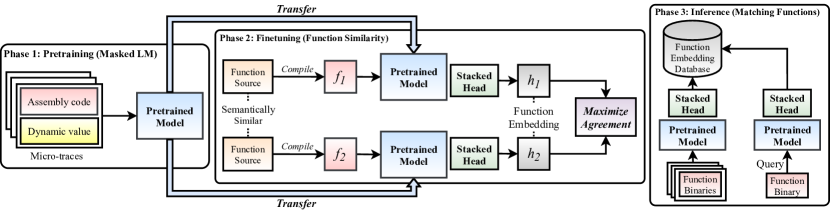
Figure 1: The workflow of Trex. We first pretrain the model on the functions’ micro-traces, consisting of both instructions and dynamic values, using the masked LM task. We then finetune the pretrained model on the semantically similar function (only static instruction) pairs by stacking new neural network layers for function similarity tasks. Finetuning updates both the pretrained model and the stacked layers. During inference, the finetuned model computes the function embedding, whose distance encodes the function similarity.

Our key observation is that while under-constrained dynamic execution traces tend to contain many infeasible states, they still encode precise execution effects of many individual instructions. Thus, we can train an ML model to observe and learn the effect of different instructions present across a large number of under-constrained dynamic traces collected from diverse functions. Once the model has gained an approximate understanding of execution semantics of various instructions, we can train it to match semantically similar functions by leveraging its learned knowledge. As a result, during inference, we do not need to execute any functions on-the-fly while matching them [45], which saves significant runtime overhead. Moreover, our trained model does not need the under-constrained dynamic traces to match functions, it only uses the function instructions, but they are augmented with rich knowledge of execution semantics.

In this paper, we extend micro-execution [34], a form of under-constrained dynamic execution, to generate micro-traces of a function across multiple instruction set architectures. A micro-trace consists of a sequence of aligned instructions and their corresponding program state values. We pretrain the model on a large number of micro-traces gathered from diverse functions as part of training data using the masked language modeling (masked LM) task. Notably, masked LM masks random parts in the sequence and asks the model to predict masked parts based on their context. This design forces the model to learn approximately how a function executes to correctly infer the missing values, which automates learning execution semantics without manual feature engineering. Masked LM is also fully self-supervised [22] – Trex can thus be trained and further improved with arbitrary functions found in the wild.

To this end, we design a hierarchical Transformer [75] that supports learning approximate execution semantics. Specifically, our architecture models micro-trace values explicitly. By contrast, existing approaches often treat the numerical values as a dummy token [50, 25] to avoid prohibitively large vocabulary size, which cannot effectively learn the rich dependencies between concrete values that likely encode key function semantics. Moreover, our architecture’s self-attention layer is designed to model long-range dependencies in a sequence [75] efficiently. Therefore, Trex can support roughly 170$\times$ longer sequence and runs 8$\times$ faster than existing neural architectures, essential to learning embeddings of long function execution traces.

We evaluate Trex on 1,472,066 functions collected from 13 popular open-source software projects across 4 architectures (x86, x64, ARM, and MIPS) and compiled with 4 optimizations (O0-O3), and 5 obfuscation strategies [78]. Trex outperforms the state-of-the-art systems by 7.8%, 7.2%, and 14.3% in matching functions across different architectures, optimizations, and obfuscations, respectively. Our ablation studies show that the pretraining task significantly improves the accuracy of matching semantically similar functions (by 15.7%). We also apply Trex in searching vulnerable functions in 180 real-world firmware images developed by well-known vendors and deployed in diverse embedded systems, including WLAN routers, smart cameras, and solar panels. Our case study shows that Trex helps find 16 CVEs in these firmware images, which have not been disclosed in previous studies. We make the following contributions.

• We propose a new approach to matching semantically similar functions: we first train the model to learn approximate program execution semantics from micro-traces, a form of under-constrained dynamic traces, and then transfer the learned knowledge to identify semantically similar functions.

• We extend micro-execution to support different architectures to collect micro-traces for training. We then develop a novel neural architecture – hierarchical Transformer – to learn approximate execution semantics from micro-traces.

• We implement Trex and evaluate it on 1,472,066 functions from 13 popular software projects and libraries. Trex outperforms the state-of-the-art tools by 7.8%, 7%, and 14.3%, in cross-architecture, optimization, and obfuscation function matching, respectively, while running up to 8$\times$ faster. Moreover, Trex helps uncover 16 vulnerabilities in 180 real-world firmware images with the latest version that are not disclosed by previous studies. We release the code and dataset of Trex at https://github.com/CUMLSec/trex.

II Overview

In this section, we use the real-world functions as motivating examples to describe the challenges of matching semantically similar functions. We then overview our approach, focusing on how our pretraining task (masked LM) addresses the challenges.

II-A Challenging Cases

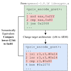
(a) Cross-architecture

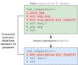
(b) Cross-optimization

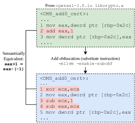
(c) Cross-obfuscation

Figure 2: Challenging cases of matching semantically similar functions across different instruction architectures, optimizations, and obfuscations. (Left) the function priv_encode_gost is from libcrypto.a in openssl-1.0.1f. The upper function is compiled to x86 while the lower is compiled to ARM. (Middle) the function <wd_comparator> is from basenc in coreutils-8.32. The upper and lower function is compiled by GCC-7.5 with -O0 and -O3, respectively. (Right) the function <CMS_add0_cert> is from libcrypto.a in openssl-1.0.1u. The upper function is compiled using clang with default options. The lower function is compiled by turning on the instruction substitution using Hikari [78], e.g., -mllvm -enable-subobf.

We use three semantically equivalent but syntactically different function pairs to demonstrate some challenges of learning from only static code. Figure 2 shows the (partial) assembly code of each function.

Cross-architecture example. Consider the functions in Figure 2a. Two functions have the same execution semantics as both functions take the lower 12-bit of a register and compare it to 0x80. Detecting this similarity requires understanding the approximate execution semantics of and in x86 and lsl/lsr in ARM. Moreover, it also requires understanding how the values (i.e., 0xfff and 0x14) in the code are manipulated. However, all existing ML-based approaches [50] only learn on static code without observing each instruction’s real execution effect. Furthermore, to mitigate the potentially prohibitive vocabulary size (i.e., all possible memory addresses), existing approaches replace all register values and memory addresses with an abstract dummy symbol [50, 26]. They thus cannot access the specific byte values to determine inherent similarity.

Cross-optimization example. Now consider two functions in Figure 2b. They are semantically equivalent as [ebp+8] and [esp+4] access the same memory location, i.e., the function’s first argument pushed on the stack by the caller. To detect such similarity, the model should understand push decreases the stack pointer esp by 4. The model should also notice that mov at line 2 assigns the decremented esp to ebp such that ebp+8 in the upper function equals esp+4 in the lower function. However, such dynamic information is not reflected in the static code.

Cross-obfuscation example. Figure 2c demonstrates a simple obfuscation by instruction substitution, which essentially replaces eax+1 with eax-(-1). Detecting the equivalence requires understanding approximately how arithmetic operations such as xor, sub, and add, executes. However, static information is not enough to expose such knowledge.

II-B Pretraining Masked LM on Micro-traces

This section describes how the pretraining task, masked LM, on functions’ micro-traces encourages the model to learn execution semantics. Although it remains an open research question to explicitly prove certain knowledge is encoded by such language modeling task [70], we focus on describing the intuition behind the masked LM – why predicting masked codes and values in micro-traces can help address the challenging cases in Figure 2.

Masked LM. Recall the operation of masked LM: given a function’s micro-trace (i.e., values and instructions), we mask some random parts and train the model to predict the masked parts using those not masked.

Note that pretraining with masked LM does not need any manual labeling effort, as it only predicts the masked part in the input micro-traces without any additional labeling effort. Therefore, Trex can be trained and further improved with a substantial number of functions found in the wild. The benefit of this is that a certain instruction not micro-executed in one function is highly likely to appear in at least one of the other functions’ micro-traces, supporting Trex to approximate diverse instructions’ execution semantics.

Masking register. Consider the functions in Figure 2c, where they essentially increment the value at stack location [rbp-0x2c] by 1. The upper function directly loads the value to eax, increments by 1, and stores the value in eax back to stack. The lower function, by contrast, takes a convoluted way by first letting ecx to hold the value -1, and decrements eax by ecx, and stores the value in eax back to stack.

We mask the eax at line 3 in the upper function. We find that our pretrained model can correctly predict its name and dynamic value. This implies the model understands the semantics of add and can deduce the value of eax in line 3 after observing the value of eax in line 2 (before the addition takes the effect). We also find the model can recover the values of masked ecx in line 4 and eax in line 5, implying the model understands the execution effect of xor and sub.

The understanding of such semantics can significantly improve the robustness in matching similar functions – when finetuned to match similar functions, the model is more likely to learn to attribute the similarity to their similar execution effects, instead of their syntactic similarity.

Masking opcode. Besides masking the register and its value, we can also mask the opcode of an instruction. Predicting the opcode requires the model to understand the execution effect of each opcode. Consider Figure 2b, where we mask mov in line 2 of upper function. We find our pretrained model predicts mov with the largest probability (larger than the other potential candidates such as add, inc, etc.).

To correctly predict the opcode, the model should have learned several key aspects of the function semantics. First, according to its context, i.e., the value of ebp at line 3 and esp at line 2, it learns mov is most probable as it assigns the value of esp to ebp. Other opcodes are less likely as their execution effect conflicts with the observed resulting register values. This also implicitly implies the model learns the approximate execution semantics of mov. Second, the model also learns the common calling convention and basic syntax of x86 instructions, e.g., only a subset of opcodes accept two operands (ebp,esp). It can thus exclude many syntactically impossible opcodes such as push, jmp, etc.

The model can thus infer ebp (line 3 of upper function) equals to esp. The model may have also learned push decrements stack pointer esp by 4 bytes, from other masked samples. Therefore, when the pretrained model is finetuned to match the two functions, the model is more likely to learn that the semantic equivalence is due to that [ebp+8] in the upper function and [esp+4] in the lower function refer to the same address, instead of their similar syntax.

Other masking strategies. Note that we are not constrained by the number or the type of items (i.e., register, opcode, etc.) in the instructions to mask, i.e., we can mask complete instructions or even a consecutive sequence of instructions, and we can mask dynamic values of random instructions’ input-output. Moreover, the masking operation dynamically selects random subsets of code blocks and program states at each training iteration and on different training samples. As a result, it enables the model to learn the diverse and composite effect of the instruction sequence, essential to detecting similarity between functions with various instructions. In this paper, we adopt a completely randomized strategy to choose what part of the micro-trace to mask with a fixed masking percentage (see Section IV-C for details). However, we envision a quite interesting future work to study a better (but still cheap) strategy to dynamically choose where and how much to mask.

III Threat Model

We assume no access to the debug symbols or source while comparing binaries. Indeed, there exist many approaches to reconstruct functions from stripped binaries [6, 72, 4, 24, 62]. Moreover, we assume the binary can be readily disassembled, i.e., it is not packed nor transformed by virtualization-based obfuscator [73, 74].

Semantic similarity. We consider two semantically similar functions as having the same input-output behavior (i.e., given the same input, two functions produce the same output). Similar to previous works [77, 50, 25], we treat functions compiled from the same source as similar, regardless of architectures, compilers, optimizations, and obfuscation transforms.

IV Methodology

This section describes Trex’s design specifics, including our micro-tracing semantics, our learning architecture’s details, and pretraining and finetuning workflow.

IV-A Micro-tracing Semantics

We implement micro-execution by Godefroid [34] to handle x64, ARM, and MIPS, where the original paper only describes x86 as the use case. In the following, we briefly explain how we micro-execute an individual function binary, highlighting the key algorithms in handling different types of instructions.

IR Language. To abstract away the complexity of different architectures’ assembly syntax, we introduce a low-level intermediate representation (IR) that models function assembly code. We only include a subset of the language specifics to illustrate the implementation algorithm. Figure 3 shows the grammar of the IR. Note that the IR here only serves to facilitate the discussion of our micro-tracing implementation. In our implementation, we use real assembly instructions and tokenize them as model’s input (Section IV-B).

Notably, we denote memory reads and writes by load($e$) and store($e_{v},e_{a}$) (i.e., store the value expression $e_{v}$ to address expression $e_{a}$), which generalize from both the load-store architecture (i.e., ARM, MIPS) and register-memory architecture (i.e., x86). Both operations can take as input $e$ – an expression that can be an explicit hexadecimal number (denoting the address or a constant), a register, or a result of an operation on two registers. We use jmp to denote the general jump instruction, which can be both direct or indirect jump (i.e., the expression $e_{a}$ can be a constant $c$ or a register $r$). The jump instruction can also be unconditional or conditional. Therefore, the first parameter in jmp is the conditional expression $e_{c}$ and unconditional jump will set $e_{c}$ to true. We represent function invocations and returns by call and ret, where call is parameterized by an expression, which can be an address (direct call) or a register (indirect call).

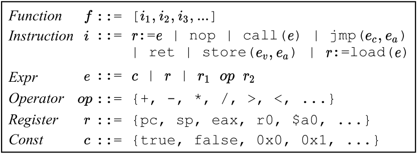
Figure 3: Low-level IR for representing assembly code. The IR abstracts away the actual assembly syntax that are disparate across different architectures.

Micro-tracing algorithm. Algorithm 1 outlines the basic steps of micro-tracing a given function $f$. First, it initializes the memory to load the code and the corresponding stack. It then initializes all registers except the special-purpose register, such as the stack pointer or the program counter. Then it starts linearly executing instructions of $f$. We map the memory address on-demand if the instruction access the memory (i.e., read/write). If the instruction reads from memory, we further initialize a random value in the specific memory addresses. For call/jump instructions, we first examine the target address and skip the invalid jump/call, known as “forced execution” [63]. By skipping unreachable jumps and calls, it can keep executing the function till the end of the function and exposes more behaviors, e.g., skipping potential input check exceptions. Since the nop instructions can serve as padding between instructions within a function, we simply skip nop. We terminate the micro-tracing when it finishes executing all instructions, reaches ret, or times out. Figure 13 and 14 demonstrate sample micro-traces of real-world functions.

IV-B Input Representation

Formally, given a function $f$ (i.e., assembly code) and its micro-trace $t$ (by micro-executing $f$), we prepare the model input $x$, consisting of 5 types of token sequence with the same size $n$. Figure 4 shows the model input example and how they are masked and processed by the hierarchical Transformer to predict the corresponding output as a pretraining task.

Algorithm 1 Micro-tracing a function $f$

Input:	Function binary $f$. All registers $r$.
Output:	Micro-trace $t$.

1:$\mathbb{I}\leftarrow get\_instructions(f)$ $\triangleright$ put all instructions in $f$ into a queue

2:$t\leftarrow empty\_vector$

3:sp $\leftarrow init\_stack\_pointer\_addr()$ $\triangleright$ stack pointer address

4:pc $\leftarrow init\_program\_counter\_addr()$ $\triangleright$ first instruction’s address

5:sm $\leftarrow mem\_map(\texttt{sp},\texttt{STACK\_SIZE})$ $\triangleright$ initialize stack memory

6:cm $\leftarrow mem\_map(\texttt{pc},|\mathbb{I}|)$ $\triangleright$ initialize memory for code

7:for each register $r_{i}$ in $r$\{sp,pc} do

8:    $r_{i}\leftarrow$ random_init() $\triangleright$ initialize register values

9:while $\mathbb{I}\neq\emptyset$ do

10:    $i$ $\leftarrow$ $dequeue(\mathbb{I})$

11:    if $i.type$ = load or $i.type$ = store then $\triangleright$ memory access

12:        $mem\_map(i.access\_addr,i.access\_size)$

13:        if $i.type$ = load then

14:           $write\_random(i.access\_addr)$         

15:        $t\leftarrow t\cup execute(i)$

16:    else if $i.type$ = jmp or $i.type$ = call then $\triangleright$ control transfer

17:        if $i.target\_addr\not\in[cm.min\_addr,cm.max\_addr]$ then

18:           continue $\triangleright$ skip illegal jump/call         

19:        $t\leftarrow t\cup execute(i)$

20:    else if $i.type$ = nop then $\triangleright$ NOP

21:        continue

22:    else if $i.type$ = ret then $\triangleright$ return

23:        break

24:    else$\triangleright$ all other instructions

25:        $t\leftarrow t\cup execute(i)$     

Micro-trace code sequence. The first sequence $x_{f}$ is the assembly code sequence: $x_{f}=\{mov,eax,+,...\}^{n}$, generated by tokenizing the assembly instructions in the micro-trace. We treat all symbols appear in the assembly instructions as tokens. Such a tokenization aims to preserve the critical hint of the syntax and semantics of the assembly instructions. For example, we consider even punctuation to be one of the tokens, e.g., “,”, “[”, “]”, as “,” implies the token before and after it as destination and source of mov (in Intel syntax), respectively, and “[” and “]” denote taking the address of the operands reside in between them.

We take special treatment of numerical values appear in the assembly code. Treating numerical values as regular text tokens can incur prohibitively large vocabulary size, e.g., $2^{32}$ number of possibilities on 32-bit architectures. To avoid this problem, we move all numeric values to the micro-trace value sequence (that will be learned by an additional neural network as detailed in the following) and replace them with a special token num (e.g., last token of input in Figure 4). With all these preprocessing steps, the vocabulary size of $x_{f}$ across all architectures is 3,300.

Micro-trace value sequence. The second sequence $x_{t}$ is the micro-trace value sequence, where each token in $x_{t}$ is the dynamic value from micro-tracing the corresponding code. As discussed in Section II, we keep explicit values (instead of a dummy value used by existing approaches) in $x_{t}$. Notably, we use the dynamic value for each token (e.g., register) in an instruction before it is executed. For example, in mov eax,0x8; mov eax,0x3, the dynamic value of the second eax is 0x8, as we take the value of eax before mov eax,0x3 is executed. For code token without dynamic value, e.g., mov, we use dummy values (see below).

Position sequences. The position of each code and value token is critical for inferring binary semantics. Unlike natural language, where swapping two words can roughly preserve the same semantic meaning, swapping two operands can significantly change the instructions. To encode the inductive bias of position into our model, we introduce instruction position sequence $x_{c}$ and opcode/operand position sequence $x_{o}$ to represent the relative positions between the instructions and within each instruction. As shown in Figure 4, $x_{c}$ is a sequence of integers encoding the position of each instruction. All opcodes/operands within a single instruction share the same value. $x_{o}$ is a sequence of integers encoding the position of each opcode and operands within a single instruction.

Architecture sequence. Finally, we feed the model with an extra sequence $x_{a}$, describing the input binary’s instruction set architecture. The vocabulary of $x_{a}$ consists of 4 architectures: $x_{a}=\{$x86, x64, ARM, MIPS$\}^{n}$. This setting helps the model to distinguish between the syntax of different architecture.

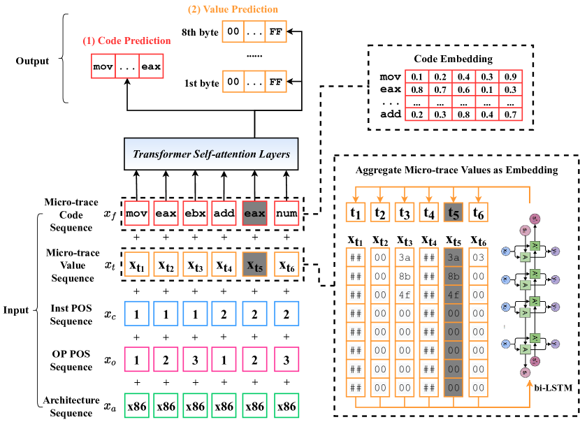
Figure 4: Model architecture with input-output example. The masked input is marked in gray. In pretraining, the loss function consists of the cross-entropy losses of both (1) code prediction and (2) value prediction, where the value prediction consists of predicting each of the 8 bytes of the micro-trace value.

Encoding numeric values. As mentioned above, treating concrete values as independent tokens can lead to prohibitively large vocabulary size. We design a hierarchical input encoding scheme to address this challenge. Specifically, let $x_{t_{i}}$ denote the $i$-th value in $x_{t}$. We represent $x_{t_{i}}$ as an (padded) 8-byte fixed-length byte sequence $x_{t_{i}}=${0x00, …, 0xff}⁸ ordered in Big-Endian. We then feed $x_{t_{i}}$ to a 2-layer bidirectional LSTM (bi-LSTM) and take its last hidden cell’s embedding as the value representation $t_{i}=bi$-$LSTM(x_{t_{i}})$. Here $t_{i}$ denotes the output of applying the embedding to $x_{t_{i}}$. To make the micro-trace code tokens without dynamic values (e.g., opcode) align with the byte sequence, we use a dummy sequence (##) with the same length. Figure 4 (right-hand side) illustrates how bi-LSTM takes the byte sequence and computes the embedding.

Such a design significantly reduces the vocabulary size as now we have only 256 possible byte values to encode. Moreover, bi-LSTM encodes the potential dependencies between high and low bytes within a single value. This setting thus supports learning better relationships between different dynamic values (e.g., memory region and offset) as opposed to treating all values as dummy tokens [71].

IV-C Pretraining with Micro-traces

This section describes the pretraining task on the function binaries and their micro-traces, focusing on how the model masks its input $x$ (5 sequences) and predicts the masked part to learn the approximate execution semantics.

Learned embeddings. We embed each token in the 5 sequences with the same embedding dimension $d_{emb}$ so that they can be summed as a single sequence as input to the Transformer. Specifically, let $E_{f}(x_{f})$, $E_{t}(x_{t})$, $E_{c}(x_{c})$, $E_{o}(x_{o})$, $E_{a}(x_{a})$ denote applying the embedding to the tokens in each sequence, respectively. We have $E_{i}$, the embedding of $x_{i}$:

$$E_{i}=E_{f}(x_{f_{i}})+E_{t}(x_{t_{i}})+E_{c}(x_{c_{i}})+E_{o}(x_{o_{i}})+E_{a}(x_{a_{i}})$$

Here $x_{f_{i}}$ denote the $i$-th token in $x_{f}$, where other sequence (i.e., $x_{t}$, $x_{c}$, $x_{o}$, $x_{a}$) follow the similar denotation. Note that $E_{t}(x_{t_{i}})$ leverages the bi-LSTM to encode the byte sequences (see Section IV-B), while the others simply multiplies the token (i.e., one-hot encoded [36]) with an embedding matrix. Figure 4 (right-hand side) illustrates the two embedding strategies.

Masked LM. We pretrain the model using the masked LM objective. Formally, for each sequence $(x_{1},x_{2},...,x_{n})$ in a given training set, we randomly mask out a selected percentage of tokens in each sequence. Specifically, we mask the code token and value token in $x_{f}$ and $x_{t}$, respectively, and replace them with a special token <MASK> (marked gray in Figure 4). As masked LM trains on micro-traces without requiring additional labels, it is fully unsupervised.

Let $m(E_{i})$ denote the embedding of the masked $x_{i}$ and $\mathbb{MP}$ a set of positions on which the masks are applied. The model $g_{p}$ (to be pretrained) takes as input a sequence of embeddings with random tokens masked: $(E_{1},...,m(E_{i}),...,E_{n}),i\in\mathbb{MP}$, and predicts the code and the values of the masked tokens: $\{\hat{x}_{f_{i}},\hat{v}_{i}|i\in\mathbb{MP}\}=g_{p}(E_{1},...,m(E_{i}),...,E_{n})$. Let $g_{p}$ be parameterized by $\theta$, the objective of training $g_{p}$ is thus to search for $\theta$ that minimizes the cross-entropy losses between (1) the predicted masked code tokens and the actual code tokens, and (2) predicted masked values (8 bytes) and the actual values. For ease of exposition, we omit summation over all samples in the training set.

$$\centering\operatorname*{arg\,min}_{\theta}\sum\limits_{i=1}^{|\mathbb{MP}|}(-x_{f_{i}}\log(\hat{x}_{f_{i}})+\alpha\sum\limits_{j=1}^{8}-x_{t_{ij}}\log(\hat{x}_{t_{ij}}))\@add@centering$$ (1)

$\hat{x}_{t_{ij}}$ denotes the predicted $j$-th byte of $x_{t_{i}}$ (the $i$-th token in $x_{t}$). $\alpha$ is a hyperparameter that weighs the cross-entropy losses between predicting code tokens and predicting values.

Masking strategy. For each chosen token to mask, we randomly choose from the masking window size from $\{1,3,5\}$, which determines how many consecutive neighboring tokens of the chosen tokens are also masked [44]. For example, if we select $x_{5}$ (the 5-th token) in Figure 4 to mask and the masking window size is 3, $x_{4}$ and $x_{6}$ will be masked too. We then adjust accordingly to ensure the overall masked tokens still account for the initially-chosen masking percentage.

Contextualized embeddings. We employ the self-attention layers [75] to endow contextual information to each embedding $E_{i}$ of the input token. Notably, let $E_{l}=(E_{l,1},...,E_{l,n})$ denote the embeddings produced by the $l$-th self-attention layer. We denote the embeddings before the model ($E_{i}$ as defined in Section IV-B) as $E_{0,i}$. Each token’s embedding at each layer will attend to all other embeddings, aggregate them, and update its embedding in the next layer. The embeddings after each self-attention layer are known as contextualized embeddings, which encodes the context-sensitive meaning of each token (e.g., eax in mov eax,ebx has different embedding with that in jmp eax). This is in contrast with static embeddings, e.g., word2vec commonly used in previous works [26, 25], where a code token is assigned to a fixed embedding regardless of the changed context.

The learned embeddings $E_{l,i}$ after the last self-attention layer encodes the approximate execution semantics of each instruction and the overall function. In pretraining, $E_{l,i}$ is used to predict the masked code. While in finetuning, it will be leveraged to match similar functions (Section IV-D).

IV-D Finetuning for Function Similarity

Given a function pair, we feed each function’s static code (instead of micro-trace as discussed in Section I) to the pretrained model $g_{p}$ and obtain the pair of embedding sequences produced by the last self-attention layer of $g_{p}$: $E^{(1)}_{k}=(E^{(1)}_{k,1},...,E^{(1)}_{k,n})$ and $E^{(2)}_{k}=(E^{(2)}_{k,1},...,E^{(2)}_{k,n})$ where $E^{(1)}_{k}$ corresponds to the first function and $E^{(2)}_{k}$ corresponds to the second. Let $y=\{-1,1\}$ be the ground-truth indicating the similarity (1 – similar, -1 – dissimilar) between two functions. We stack a 2-layer Multi-layer Perceptrons $g_{t}$, taking as input the average of embeddings for each function, and producing a function embedding:

$$g_{t}(E_{k})=tanh((\sum\limits_{i=1}^{n}E_{k,i})/n)\cdot W_{1})\cdot W_{2}$$

Here $W_{1}\in\mathbb{R}^{d_{emb}\times d_{emb}}$ and $W_{2}\in\mathbb{R}^{d_{emb}\times d_{func}}$ transforms the average of last self-attention layers embeddings $E_{k}$ with dimension $d_{emb}$ into the function embedding with the dimension $d_{func}$. $d_{func}$ is often chosen smaller than $d_{emb}$ to support efficient large-scale function searching [77]. Now let $g_{t}$ be parameterized by $\theta$, the finetuning objective is to minimize the cosine embedding loss ($l_{ce}$) between the ground-truth and the cosine distance between two function embeddings:

$$\operatorname*{arg\,min}_{\theta}\ l_{ce}(g_{t}(E^{(1)}_{k}),g_{t}(E^{(2)}_{k}),y)$$

where

$$l_{ce}(x_{1},x_{2},y)=\left\{\begin{matrix}1-cos(x_{1},x_{2})&y=1\\ max(0,cos(x_{1},x_{2})-\xi)&y=-1\end{matrix}\right.$$ (2)

$\xi$ is the margin usually chosen between 0 and 0.5 [59]. As both $g_{p}$ and $g_{t}$ are neural nets, optimizing Equation 1 and Equation 2 can be guided by gradient descent via backpropagation.

After finetuning $g_{t}$, the 2-layer multilayer perceptrons, and $g_{p}$, the pre-trained model, we compute the function embedding $f_{emb}=g_{t}(g_{p}(f))$ and the similarity between two functions is measured by the cosine similarity between two function embedding vectors: $cos(f^{(1)}_{emb},f^{(2)}_{emb})$.

V Implementation and Experimental Setup

We implement Trex using fairseq, a sequence modeling toolkit [55], based on PyTorch 1.6.0 with CUDA 10.2 and CUDNN 7.6.5. We run all experiments on a Linux server running Ubuntu 18.04, with an Intel Xeon 6230 at 2.10GHz with 80 virtual cores including hyperthreading, 385GB RAM, and 8 Nvidia RTX 2080-Ti GPUs.

Datasets. To train and evaluate Trex, we collect 13 popular open-source software projects. These projects include Binutils-2.34, Coreutils-8.32, Curl-7.71.1, Diffutils-3.7, Findutils-4.7.0, GMP-6.2.0, ImageMagick-7.0.10, Libmicrohttpd-0.9.71, LibTomCrypt-1.18.2, OpenSSL-1.0.1f and OpenSSL-1.0.1u, PuTTy-0.74, SQLite-3.34.0, and Zlib-1.2.11. We compile these projects into 4 architectures i.e., x86, x64, ARM (32-bit), and MIPS (32-bit), with 4 optimization levels (OPT), i.e., O0, O1, O2, and O3, using GCC-7.5. Specifically, we compile the software projects based on its makefile, by specifying CFLAGS (to set optimization flag), CC (to set cross-compiler), and --host (to set the cross-compilation target architecture). We always compile to dynamic shared objects, but resort to static linking when we encounter build errors. We are able to compile all projects with these treatments.

We also obfuscate all projects using 5 types of obfuscations (OBF) by Hikari [78] on x64 – an obfuscator based on clang-8. The obfuscations include bogus control flow (bcf), control flow flattening (cff), register-based indirect branching (ibr), basic block splitting (spl), and instruction substitution (sub). As we encounter several errors in cross-compilation using Hikari (based on Clang) [78], and the baseline system (i.e., Asm2Vec [25]) to which we compare only evaluates on x64, we restrict the obfuscated binaries for x64 only. As a result, we have 1,472,066 functions, as shown in Table I.

TABLE I: Number of functions for each project across 4 architectures with 4 optimization levels and 5 obfuscations.

ARCH	OPT OBF	# Functions
		Binutils	Coreutils	Curl	Diffutils	Findutils	GMP	ImageMagick	Libmicrohttpd	LibTomCrypt	OpenSSL	PuTTy	SQLite	Zlib	Total
	O0	25,492	19,992	1,067	944	1,529	766	2,938	200	779	11,918	7,087	2,283	157	75,152
	O1	20,043	14,918	771	694	1,128	704	2,341	176	745	10,991	5,765	1,614	143	60,033
	O2	19,493	14,778	765	693	1,108	701	2,358	171	745	11,001	5,756	1,473	138	59,180
	O3	17,814	13,931	697	627	983	680	2,294	160	726	10,633	5,458	1,278	125	55,406
ARM	Total # Functions of ARM														249,771
MIPS	O0	28,460	18,843	1,042	906	1,463	734	2,840	200	779	11,866	7,003	2,199	153	76,488
	O1	22,530	13,771	746	653	1,059	670	2,243	176	745	10,940	5,685	1,530	139	60,887
	O2	22,004	13,647	741	653	1,039	667	2,260	171	743	10,952	5,677	1,392	135	60,081
	O3	20,289	12,720	673	584	917	646	2,198	161	724	10,581	5,376	1,197	121	56,187
	Total # Functions of MIPS														253,643
	O0	37,783	24,383	1,335	1,189	1,884	809	3,876	326	818	12,552	7,548	2,923	204	95,630
	O1	32,263	20,079	1,013	967	1,516	741	3,482	280	782	11,578	6,171	2,248	196	81,316
	O2	32,797	21,082	1,054	1,006	1,524	728	3,560	265	784	11,721	6,171	2,113	183	82,988
	O3	34,055	22,482	1,020	1,052	1,445	707	3,597	284	760	11,771	5,892	1,930	197	85,192
x86	Total # Functions of x86														358,261
x64	O0	26,757	17,238	1,034	845	1,386	751	2,970	200	782	12,047	7,061	2,190	151	73,412
	O1	21,447	12,532	739	600	1,000	691	2,358	176	745	11,120	5,728	1,523	137	58,796
	O2	20,992	12,206	734	596	976	689	2,374	171	742	11,136	5,703	1,380	132	57,831
	O3	19,491	11,488	662	536	857	667	2,308	160	725	10,768	5,390	1,183	119	54,354
	Total # Functions of x64														244,393
	bcf	27,734	17,093	998	840	1,388	746	2,833	200	782	10,768	7,069	2,183	151	72,785
	cff	27,734	17,093	998	840	1,388	746	2,833	200	782	10,903	7,069	2,183	151	72,920
	ibr	27,734	17,105	998	842	1,392	746	2,833	204	782	12,045	7,069	2,183	151	74,084
	spl	27,734	17,093	998	840	1,388	746	2,833	200	782	10,772	7,069	2,183	151	72,789
	sub	27,734	17,093	998	840	1,388	746	2,833	200	782	11,403	7,069	2,183	151	73,420
x64	Total # Obfuscated Functions														365,998
Total # Functions															1,472,066

Micro-tracing. We implement micro-tracing by Unicorn [66], a cross-platform CPU emulator based on QEMU [8]. We micro-execute each function 3 times with different initialized registers and memory, generating 3 micro-traces (including both static code and dynamic values) for pretraining (masked LM). We leverage multi-processing to parallelize micro-executing each function and set 30 seconds as the timeout for each run in case any instruction gets stuck (i.e., infinite loops). For each function (with 3 micro-traces), we append one additional dummy trace, which consists of only dummy values (##). This setting encourages the model to leverage its learned execution semantics (from other traces with concrete dynamic values) to predict the masked code with only code context, which helps the finetuning task as we only feed the functions’ static code as input (discussed in Section I).

Baselines. For comparing cross-architecture performance, we consider 2 state-of-the-art systems. The first one is SAFE [50] that achieves state-of-the-art function matching accuracy. As SAFE’s trained model is publicly available, we compare Trex with both SAFE’s reported results on their dataset, i.e., OpenSSL-1.0.1f and OpenSSL-1.0.1u, and running their trained models on all of our collected binaries. The second baseline is Gemini [77], which is shown outperformed by SAFE. As Gemini does not release their trained models, we compare our results to their reported numbers directly on their evaluated dataset, i.e., OpenSSL-1.0.1f and OpenSSL-1.0.1u.

For cross-optimization/obfuscation comparison, we consider Asm2Vec [25] and Blex [27] as the baselines. Asm2Vec achieves the state-of-the-art cross-optimization/obfuscation results, based on learned embeddings from static assembly code. Blex, on the other hand, leverages functions’ dynamic behavior to match function binaries. As we only find a third-party implementation of Asm2Vec that achieves extremely low Precision@1 (the metric used in Asm2Vec) from our testing (e.g., 0.02 vs. their reported 0.814), and we have contacted the authors and do not get replies, we directly compare to their reported numbers. Blex is not publicly available either, so we also compare to their reported numbers directly.

Metrics. As the cosine similarity between two function embeddings can be an arbitrary real value between -1 and 1, there has to be a mechanism to threshold the similarity score to determine whether the function pairs are similar or dissimilar. The chosen thresholds largely determine the model’s predictive performance [57]. To avoid the potential bias introduced by a specific threshold value, we consider the receiver operating characteristic (ROC) curve, which measures the model’s false positives/true positives under different thresholds. Notably, we use the area under curve (AUC) of the ROC curve to quantify the accuracy of Trex to facilitate benchmarking – the higher the AUC score, the better the model’s accuracy.

Certain baselines do not use AUC score to evaluate their system. For example, Asm2Vec uses Precision at Position 1 (Precision@1), and Blex uses the number of matched functions as the metric. Therefore, we also include these metrics to evaluate Trex when needed. Specifically, given a sequence of query functions and the target functions to be matched, Precision@1 measures the percentage of matched query functions in the target functions. Here “match” means the query function should have the top-1 highest similarity score with the ground truth function among the target functions.

To evaluate pretraining performance, we use the standard metric for evaluating the language model – perplexity (PPL). The lower the PPL the better the pretrained model in predicting masked code. The lowest PPL is 1.

Pretraining setup. To strictly separate the functions in pretraining, finetuning, and testing, we pretrain Trex on all functions in the dataset, except the functions in the project going to be finetuned and evaluated for similarity. For example, the function matching results of Binutils (Table II) are finetuned on the model pretrained on all other projects without Binutils.

Note that pretraining is agnostic to any labels (e.g., ground-truth indicating similar functions). Therefore, we can always pretrain on large-scale codebases, which can potentially include the functions for finetuning (this is the common practice in transfer learning [22]). It is thus worth noting that our setup of separating functions for pretraining and finetuning makes our testing significantly more challenging.

We keep the pretrained model weights that achieve the best validation PPL for finetuning. The validation set for pretraining consists of 10,000 random functions selected from Table I.

Finetuning setup. We choose 50,000 random function pairs for each project and randomly select only 10% for training, and the remaining is used as the testing set. We keep the training and testing functions strictly non-duplicated by ensuring the functions that appear in training function pairs not appear in the testing. As opposed to the typical train-test split (e.g., 80% training and 20% testing [50]), our setting requires the model to generalize from few training samples to a large number of unseen testing samples, which alleviates the possibility of overfitting. Moreover, we keep the ratio between similar and dissimilar function pairs in the finetuning set as roughly 1:5. This setting follows the practice of contrastive learning [70, 15], respecting the actual distribution of similar/dissimilar functions as the number of dissimilar functions is often larger than that of similar functions in practice.

Hyperparameters. We pretrain and finetune the models for 10 epochs and 30 epochs, respectively. We choose $\alpha=0.125$ in Equation 1 such that the cross-entropy loss of code prediction and value prediction have the same weight. We pick $\xi=0.1$ in Equation 2 to make the model slightly inclined to treat functions as dissimilar because functions in practice are mostly dissimilar. We fix the largest input length to be 512 and split the functions longer than this length into subsequences for pretraining. We average the subsequences’ embeddings during finetuning if the function is split to more than one subsequences. In this paper, we keep most of the hyperparameters fixed throughout the evaluation if not mentioned explicitly (complete hyperparameters are defined in Appendix -B). While we can always search for better hyperparameters, there is no principled method to date [9]. We thus leave as future work a more thorough study of Trex’s hyperparameters.

VI Evaluation

Our evaluation aims to answer the following questions.

• RQ1: How accurate is Trex in matching semantically similar function binaries across different architectures, optimizations, and obfuscations?

• RQ2: How does Trex compare to the state-of-the-art?

• RQ3: How fast is Trex compared to other tools?

• RQ4: How much does pretraining on micro-traces help improve the accuracy of matching functions?

TABLE II: Trex results (in AUC score) on function pairs across architectures, optimizations, and obfuscations.

	Cross-
	ARCH	OPT	OBF	ARCH+ OPT	ARCH+ OPT+ OBF
Binutils	0.993	0.993	0.991	0.959	0.947
Coreutils	0.991	0.992	0.991	0.956	0.945
Curl	0.993	0.993	0.991	0.958	0.956
Diffutils	0.992	0.992	0.990	0.970	0.961
Findutils	0.990	0.992	0.990	0.965	0.963
GMP	0.992	0.993	0.990	0.968	0.966
ImageMagick	0.993	0.993	0.989	0.960	0.951
Libmicrohttpd	0.994	0.994	0.991	0.972	0.969
LibTomCrypt	0.992	0.994	0.991	0.981	0.970
OpenSSL	0.992	0.992	0.989	0.964	0.956
PuTTy	0.992	0.995	0.990	0.961	0.952
SQLite	0.991	0.994	0.993	0.980	0.959
Zlib	0.990	0.991	0.990	0.979	0.965
Average	0.992	0.993	0.990	0.967	0.958

VI-A RQ1: Accuracy

We evaluate how accurate Trex is in matching similar functions across different architectures, optimizations, and obfuscations. As shown in Table II, we prepare function pairs for each project (first column) with 5 types of partitions. (1) ARCH: the function pairs have different architectures but same optimizations without obfuscations (2nd column). (2) OPT: the function pairs have different optimizations but same architectures without obfuscations (3rd column). (3) OBF: the function pairs have different obfuscations with same architectures (x64) and no optimization (4th column). (4) ARCH+OPT: the function pairs have both different architectures and optimizations without obfuscations (5th column). (5) ARCH+OPT+OBF: the function pairs can come from arbitrary architectures, optimizations, and obfuscations (6th column).

Table II reports the mean testing AUC scores of Trex on each project with 3 runs. On average, Trex achieves $>0.958$ (and up to 0.995) AUC scores, even in the most challenging setting where the functions can come from different architectures, optimizations, and obfuscations at the same time. We note that Trex performs the best on cross-optimization matching. This is intuitive as the syntax of two functions from different optimizations are not changed significantly (e.g., the name of opcode, operands remain the same). Nevertheless, we find the AUC scores for matching functions from different architectures is only 0.001 lower, which indicates the model is robust to entirely different syntax between two architectures. On matching functions with different obfuscations, Trex’s results are 0.026, on average, lower than that of cross-optimizations, which indicates the obfuscation changes the code more drastically. Section VI-B will show the specific results of Trex on each obfuscations.

VI-B RQ2: Baseline Comparison

Cross-architecture search. As described in Section V, we first compare Trex with SAFE and Gemini on OpenSSL-1.0.1f and OpenSSL-1.0.1u with their reported numbers (as they only evaluate on these two projects). We then run SAFE’s released model on our dataset and compare to Trex.

We use our testing setup (see Section V) to evaluate SAFE’s trained model, where 90% of the total functions of those in Table I are used to construct the testing set. These testing sets are much larger than that in SAFE, where they only evaluate on 20% of the OpenSSL functions. Note that the dataset used in SAFE are all compiled by GCC-5.4 at the time when it is publicized (November 2018), while ours are compiled by GCC-7.5 (April 2020). We find these factors (the more diverse dataset and different compilers) can all lead to the possible dataset distribution shift, which often results in the decaying performance of ML models when applied in the security applications [43].

To study the distribution shift, we measure the KL-divergence [48] between SAFE’s dataset (OpenSSL compiled by GCC-5.4) and our dataset. Specifically, we use the probability distribution of the raw bytes of the compiled projects’ binaries, and compute their KL-divergence between SAFE and ours. As OpenSSL is also a subset of our complete dataset, we compute the KL-divergence between our compiled OpenSSL and that of SAFE as the baseline.

We find the KL-divergence is 0.02 between SAFE’s dataset and ours, while it decreases to 0.0066 between our compiled OpenSSL and that of SAFE. This indicates that the underlying distribution of our test set shifts from that of SAFE’s. Moreover, the KL-divergence of 0.0066 between the same dataset (OpenSSL) but only compiled by different GCC versions implies that the compiler version has much smaller effect to the distribution shift than the different software projects.

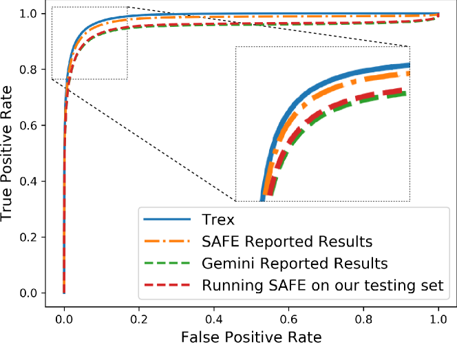
Figure 5: ROC curves of matching functions in OpenSSL across different architectures. Trex outperforms the reported results of SAFE and Gemini and the results of running SAFE’s trained model on our testing set.

As shown in Figure 5, our ROC curve is higher than those reported in SAFE and Gemini. While SAFE’s reported AUC score, 0.992, is close to ours, when we run their trained model on our testing set, its AUC score drops to 0.976 – possibly because our testing set is much larger than theirs. This observation demonstrates the generalizability of Trex– when pretrained to approximately learn execution semantics explicitly, it can quickly generalize to match unseen (semantically similar) functions with only a minimal training set.

Figure 6: Comparison between Trex and SAFE on matching functions in each project compiled to different architectures (see Table I).

Figure 6 shows that Trex consistently outperforms SAFE on all projects, i.e., by 7.3% on average. As the SAFE’s model is only trained on OpenSSL, we also follow the same setting by training Trex on only OpenSSL, similar to the cross-project setting described in Section VI-A.

Cross-optimization search. We compare Trex with Asm2Vec and BLEX on matching functions compiled by different optimizations. As both Asm2vec and Blex run on single architecture, we restrict the comparison on x64. Besides, since Asm2Vec uses Precision@1 and Blex uses accuracy as the metric (discussed in Section V), we compare with each tool separately using their metrics and on their evaluated dataset.

TABLE III: Comparison between Trex and Asm2Vec (in Precision@1) on function pairs across optimizations.

	Cross Compiler Optimization
	O2 and O3		O0 and O3
	Trex	Asm2Vec	Trex	Asm2Vec
Coreutils	0.955	0.929	0.913	0.781
Curl	0.961	0.951	0.894	0.850
GMP	0.974	0.973	0.886	0.763
ImageMagick	0.971	0.971	0.891	0.837
LibTomCrypt	0.991	0.991	0.923	0.921
OpenSSL	0.982	0.931	0.914	0.792
PuTTy	0.956	0.891	0.926	0.788
SQLite	0.931	0.926	0.911	0.776
Zlib	0.890	0.885	0.902	0.722
Average	0.957	0.939	0.907	0.803

Table III shows Trex outperforms Asm2Vec in Precision@1 (by 7.2% on average) on functions compiled by different optimizations (i.e., between O2 and O3 and between O0 and O3). As the syntactic difference introduced by optimizations between O0 and O3 is more significant than that between O2 and O3, both tools have certain level of decrease in AUC scores (5% drop for Trex and 14% for Asm2Vec), but Trex’s AUC score drops much less than that of Asm2Vec.

To compare to Blex, we evaluate Trex on Coreutils between optimizations O0 and O3, where they report to achieve better performance than BinDiff [79]. As Blex show the matched functions of each individual utility in Coreutils in a barchart without including the concrete numbers of matched functions, we estimate their matched functions using their reported average percentage (75%) on all utilities.

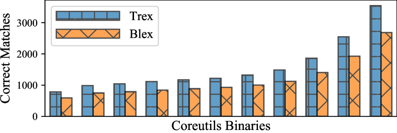
Figure 7: Cross-optimization function matching between O0 and O3 on Coreutils by Trex and Blex. We sort the 109 utility binaries in Coreutils by their number of functions, and aggregate the matched functions every 10 utilities.

Figure 7 shows that Trex consistently outperforms Blex in number of matched functions in all utility programs of Coreutils. Note that Blex also executes the function and uses the dynamic features to match binaries. The observation here thus implies that the learned execution semantics from Trex is more effective than the hand-coded features in Blex for matching similar binaries.

Cross-obfuscation search. We compare Trex to Asm2Vec on matching obfuscated function binaries with different obfuscation methods. Notably, Asm2Vec is evaluated on obfuscations including bogus control flow (bcf), control flow flattening (cff), and instruction substitution (sub), which are subset of our evaluated obfuscations (Table I). As Asm2Vec only evaluates on 4 projects, i.e., GMP, ImageMagic, LibTomCrypt, and OpenSSL, we focus on these 4 projects and Trex’s results for other projects are included in Table II.

TABLE IV: Comparison between Trex and Asm2Vec (in Precision@1) on function pairs across differet obfuscations.

		GMP	LibTomCrypt	ImageMagic	OpenSSL	Average
	Trex	0.926	0.938	0.934	0.898	0.924
bcf	Asm2Vec	0.802	0.920	0.933	0.883	0.885
ccf	Trex	0.943	0.931	0.936	0.940	0.930
	Asm2Vec	0.772	0.920	0.890	0.795	0.844
	Trex	0.949	0.962	0.981	0.980	0.968
sub	Asm2Vec	0.940	0.960	0.981	0.961	0.961
All	Trex	0.911	0.938	0.960	0.912	0.930
	Asm2Vec	0.854	0.880	0.830	0.690	0.814

Table IV shows Trex achieves better Precision@1 score (by 14.3% on average) throughout all different obfuscations. Importantly, the last two rows show when multiple obfuscations are combined, Trex performance is not dropping as significant as Asm2Vec. It also shows Trex remains robust under varying obfuscations with different difficulties. For example, instruction substitution simply replaces very limited instructions (i.e., arithmetic operations as shown in Section II) while control flow flattening dramatically changes the function code. Asm2Vec has 12.2% decreased score when the obfuscation is changed from sub to ccf, while Trex only decreases by 4%.

VI-C RQ3: Execution Time

We evaluate the runtime performance of generating function embeddings for computing similarity. We compare Trex with SAFE and Gemini on generating functions in 4 projects on x64 compiled by O3, i.e., Binutils, Putty, Findutils, and Diffutils, which have disparate total number of functions (see Table I. This tests how Trex scales to different number of functions compared to other baselines. Since the offline training (i.e., pretraining Trex) of all the learning-based tools is a one-time cost, it can be amortized in the function matching process so we do not explicitly measure the training time. Moreover, the output of all tools are function embeddings, which can be indexed and efficiently searched using locality sensitive hashing (LSH) [33, 67]. Therefore, we do not compare the matching time of function embeddings as it simply depends on the performance of underlying LSH implementation.

Particularly, we compare the runtime of two procedures in matching functions. (1) Function parsing, which transforms the function binaries into the format that the model needs. (2) Embedding generation, which takes the parsed function binary as input and computes function embedding. We test the embedding generation using our GPU (see Section V).

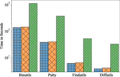
(a) Function parsing

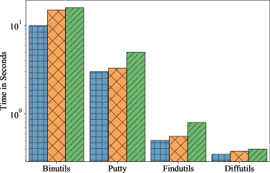
(b) Embedding generation

Figure 8: Runtime performance (lower is better) of Trex, SAFE, and Gemini on (a) function parsing and (b) embedding generation. The time is log-scaled.

Figure 8 shows that Trex is more efficient than the other tools in both function parsing and embedding generation for functions from 4 different projects with different number of functions (Table I). Gemini requires manually constructing control flow graph and extracting inter-/intra-basic-block feature engineering. It thus incurs the largest overhead. For generating function embeddings, our underlying network architectures leverage Transformer self-attention layers, which is more amenable to parallezation with GPU than the recurrent (used by SAFE) and graph neural network (used by Gemini) [75]. As a result, Trex runs up to 8$\times$ faster than SAFE and Gemini.

VI-D RQ4: Ablation Study

In this section, we aim to quantify how much each key component in Trex’s design helps the end results. We first study how much does pretraining, argued to assist learning approximate execution semantics, help match function binaries. We then study how does pretraining without micro-traces affect the end results. We also test how much does incorporating the micro-traces in the pretraining tasks improve the accuracy.

Pretraining effectiveness. We compare the testing between AUC scores achieved by Trex (1) with pretraining (except the target project that will be finetuned), (2) with 66% of pretraining functions in (1), (3) with 33% of pretraining functions in (1), and (4) without pretraining (the function embedding is computed by randomly-initialized model weights that are not pretrained). The function pairs can come from arbitrary architectures, optimizations, and obfuscations.

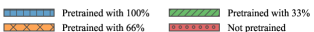
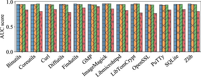
Figure 9: Comparison of testing AUC scores between models pretrained with different fraction of the pretraining set.

Figure 9 shows that the model’s AUC score drops significantly (on average 15.7%) when the model is not pretrained. Interestingly, we observe that the finetuned models achieve similar AUC scores, i.e., with only 1% decrease when pretrained with 33% of the functions compared to pretraining with all functions. This indicates that we can potentially decrease our pretraining data size to achieve roughly the same performance. However, since our pretraining task does not require collect any label, we can still collect unlimited binary code found in the wild to enrich the semantics that can be observed.

Pretraining w/o micro-traces. We try to understand whether including the micro-traces in pretraining can really help the model to learn better execution semantics than learning from only static assembly code, which in turn results in better function matching accuracy. Specifically, we pretrain the model on the data that contains only dummy value sequence (see Section IV), and follow the same experiment setting as described above. Besides replacing the input value sequence as dummy value, we accordingly remove the prediction of dynamic values in the pretraining objective (Equation 1). We also compare to SAFE in this case.

Figure 10 shows that the AUC scores decrease by 7.2% when the model is pretrained without micro-trace. The AUC score of pretrained Trex without micro-traces is even 0.035 lower than that of SAFE. However, the model still performs reasonably well, achieving 0.88 AUC scores even when the functions can come from arbitrary architectures, optimizations, and obfuscations. Moreover, we observe that pretraining without micro-traces has less performance drop than the model simply not pretrained (7.2% vs. 15.7%). This demonstrates that even pretraining with only static assembly code is indeed helpful to improve matching functions. One possible interpretation is that similar functions are statically similar in syntax, while understanding their inherently similar execution semantics just further increases the similarity score.

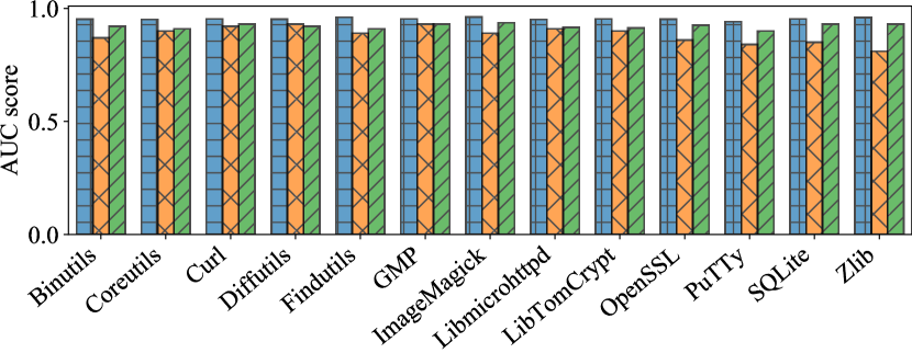
Figure 10: Comparison of testing AUC scores between models pretrained with micro-trace and pretrained without micro-trace.

Pretraining accuracy. We study the testing perplexity (PPL defined in Section V) of pretraining Trex to directly validate whether it indeed helps Trex to learn the approximate execution semantics. The rationale is the good performance, i.e., the low PPL, on unseen testing function binaries indicates that Trex highly likely learns to generalize based on its learned approximate execution semantics.

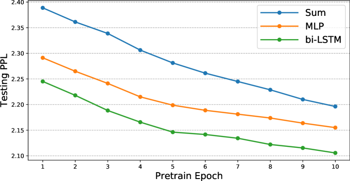
Figure 11: Testing PPL of pretraining Trex in 10 epochs. We compare different designs of combining byte-sequence in the micro-trace (see Section IV-B).

The green line in Figure 11 shows the validation PPL in 10 epochs of pretraining Trex. The testing set is constructed by sampling 10,000 random functions from the projects used in pretraining (as described in Section V). We observe that the PPL of Trex drops to close to 2.1, which is far below that of random guessing (e.g., random guessing PPL is $2^{-\log(1/256)}=256$), indicating that Trex has around 0.48 confidence on average on the masked tokens being the correct value. Note that a random guessing has only 1/256=0.004 confidence on the masked tokens being the correct value.

VII Case Studies

In this section, we study how Trex can help discover new vulnerabilities in a large volume of latest firmware images.

TABLE V: Vulnerabilities we have confirmed (✓) in firmware images (latest version) from 4 well-known vendors and products.

CVE	Ubiquiti sunMax	TP-Link Deco-M4	NETGEAR R7000	Linksys RE7000
CVE-2019-1563	✓	✓	✓	✗
CVE-2017-16544	✗	✓	✗	✗
CVE-2016-6303	✓	✓	✓	✓
CVE-2016-6302	✓	✓	✓	✓
CVE-2016-2842	✓	✓	✓	✓
CVE-2016-2182	✓	✓	✓	✓
CVE-2016-2180	✓	✓	✓	✓
CVE-2016-2178	✓	✓	✓	✓
CVE-2016-2176	✓	✓	✗	✓
CVE-2016-2109	✓	✓	✗	✓
CVE-2016-2106	✓	✓	✗	✓
CVE-2016-2105	✓	✓	✗	✓
CVE-2016-0799	✓	✓	✗	✓
CVE-2016-0798	✓	✓	✗	✓
CVE-2016-0797	✓	✓	✗	✓
CVE-2016-0705	✓	✓	✗	✓

Firmware images often include third-party libraries (i.e., BusyBox, OpenSSL). However, these libraries are frequently patched, but the manufacturers often fall behind to update them accordingly [56]. Therefore, we study whether our tool can uncover function binaries in firmware images similar to known vulnerable functions. We find existing state-of-the-art binary similarity tools (i.e., SAFE [50], Asm2Vec [25], Gemini [77]) all perform their case studies on the firmware images and vulnerabilities that have already been studied before them [17, 30, 19, 14]. Therefore, we decide to collect our own dataset with more updated firmware images and the latest vulnerabilities, instead of reusing the existing benchmarks. This facilitates finding new (1-day) vulnerabilities in most recent firmware images that are not disclosed before.

We crawl firmware images (in their latest version) in 180 products including WLAN routers, smart cameras, and solar panels, from well-known manufacturers’ official releases and third-party providers such as DD-WRT [35], as shown in Table VIII. We collect firmware images with only the latest version, which are much more updated than those studied in the state-of-the-art (dated before 2015, which are all patched before their studies). For each function in the firmware images, we construct function embedding and build a firmware image database using Open Distro for Elasticsearch [3], which supports vector-based indexing with efficient search support based on NMSLIB [11].

We extract the firmware images using binwalk [23]. In total, we collect 180 number of firmware images from 22 vendors. These firmware images are developed by the original vendors, or from third-party providers such as DD-WRT [35]. Most of them are for WLAN routers, while some are deployed in other embedded systems, such as solar panels and smart cameras. Among the firmware images, 127 of them are compiled for MIPS 32-bit and 53 are compiled for ARM 32-bit. 169 of them are 2020 models, and the rest are 2019 and 2018 models.

TABLE VI: We study 16 vulnerabilities from OpenSSL and BusyBox, two widely-used libraries in firmware images.

CVE	Library	Description
CVE-2019-1563	OpenSSL	Decrypt encrypted message
CVE-2017-16544	BusyBox	Allow executing arbitrary code
CVE-2016-6303	OpenSSL	Integer overflow
CVE-2016-6302	OpenSSL	Allows denial-of-service
CVE-2016-2842	OpenSSL	Allows denial-of-service
CVE-2016-2182	OpenSSL	Allows denial-of-service
CVE-2016-2180	OpenSSL	Out-of-bounds read
CVE-2016-2178	OpenSSL	Leak DSA private key
CVE-2016-2176	OpenSSL	Buffer over-read
CVE-2016-2109	OpenSSL	Allows denial-of-service
CVE-2016-2106	OpenSSL	Integer overflow
CVE-2016-2105	OpenSSL	Integer overflow
CVE-2016-0799	OpenSSL	Out-of-bounds read
CVE-2016-0798	OpenSSL	Allows denial-of-service
CVE-2016-0797	OpenSSL	NULL pointer dereference
CVE-2016-0705	OpenSSL	Memory corruption

Table V shows 16 vulnerabilities (CVEs) we use to search in the firmware images. We focus on the CVEs of OpenSSL and BusyBox, as they are widely included in the firmware. For each CVE, we compile the corresponding vulnerable functions in the specified library version and computes the vulnerable function embeddings via Trex. As the firmware images are stripped so that we do not know with which optimizations they are compiled, we compile the vulnerable functions to both MIPS and ARM with -O3 and rely on Trex’s capability in cross-architecture and optimization function matching to match functions that are potentially compiled in different architectures and with different optimizations. We then obtain the firmware functions that rank top-10 similar to the vulnerable function and manually verify if they are vulnerable. We leverage strings command to identify the OpenSSL and BusyBox versions indicative of the corresponding vulnerabilities. Note that such information can be stripped for other libraries so it is not a reliable approach in general. As shown in Table V, we have confirmed all 16 CVEs in 4 firmware models developed by well-known vendors, i.e., Ubiquiti, TP-Link, NETGEAR, and Linksys. These cases demonstrate the practicality of Trex, which helps discover real-world vulnerabilities in large-scale firmware databases. Table VI shows the details of the 16 vulnerabilities that Trex uncover in the 4 firmware images shown in Table V. The description of “allow denial-of-service” usually refers to the segmentation fault that crashes the program. The cause of such error can be diverse, which is not due to the other typical causes shown in the table (e.g., integer overflow, buffer over-read, etc.).

VIII Related Work

VIII-A Binary Similarity

Traditional approaches. Existing static approaches often extract hand-crafted features by domain experts to match similar functions. The features often encode the functions’ syntactic characteristics. For example, BinDiff [79] extracts the number of basic blocks and the number of function calls to determine the similarity. Other works [54, 47, 18, 29] introduce more carefully-selected static features such as n-gram of instruction sequences. Another popular approach is to compute the structural distance between functions to determine the similarity [79, 10, 21, 65, 28, 20, 40]. For example, BinDiff [79] performs graph matching between functions’ call graphs. TEDEM [65] matches the basic block expression trees. BinSequence [40] and Tracelet [21] uses the edit distance between functions’ instruction sequence. As discussed in Section I, both static features and structures are susceptible to obfuscations and optimizations and incur high overhead. Trex automates learning approximate execution semantics without any manual effort, and the execution semantics is more robust to match semantically similar functions.

In addition to the static approaches, dynamic approaches such as iLine [41], BinHunt [52], iBinHunt [52], Revolver [45], Blex [27], Rieck et al. [69], Multi-MH [64], BinGo [13], ESH [19], BinSim [53], CACompare [39], Vulseeker-pro [32], and Tinbergen [51] construct hand-coded dynamic features, such as values written to stack/heap [27] or system calls [53] by executing the function to match similar functions. These approaches can detect semantically similar (but syntactically different) functions by observing their similar execution behavior. However, as discussed in Section I, these approaches can be expensive and can suffer from false positives due to the under-constrained dynamic execution traces [42, 25]. By contrast, we only use these traces to learn approximate execution semantics of individual instructions and transfer the learned knowledge to match similar functions without directly comparing their dynamic traces. Therefore, we are much more efficient and less susceptible to the imprecision introduced by these under-constrained dynamic traces.

Learning-based approaches. Most recent learning-based works such as Genius [30], Gemini [77], Asm2Vec [25], SAFE [50], DeepBinDiff [26] learn a function representation that is supposed to encode the function syntax and semantics in low dimensional vectors, known as function embeddings. The embeddings are constructed by learning a neural network that takes the functions’ structures (control flow graph) [30, 77, 26] or instruction sequences [25, 50] as input and train the model to align the function embedding distances to the similarity scores. All existing approaches are based only on static code, which lacks the knowledge of function execution semantics. Moreover, the learning architectures adopted in these approaches require constructing expensive graph features (attributed CFG [30, 77]) or limited in modeling long-range dependencies (based on Word2Vec [25, 26]). By contrast, Trex learns approximate execution semantics to match functions. Its underlying architecture is amenable to learning long-range dependencies in sequences without heavyweight feature engineering or graph construction.

VIII-B Learning Program Representations

There has been a growing interest in learning neural program representation as embeddings from “Big Code” [2]. The learned embedding of the code encodes the program’s key properties (i.e., semantics, syntax), which can be leveraged to perform many applications beyond function similarity, such as program repair [58, 76], recovering symbol names and types [16, 60], code completion [68], decompilation [31, 46], prefetching [71], and many others that we refer to Allamanis et al. [2] for a more thorough list. Among these works, the most closest work to us is XDA [62], which also leverages the transfer learning to learn general program representations for recovering function and instruction boundaries. However, XDA only learns from static code at the raw byte level, which lacks the understanding of execution semantics.

The core technique proposed in this paper – learning approximate execution semantics from micro-traces – is by no means limited to only function similarity task but can be applied to any of the above tasks. Indeed, we plan to explore how the learned semantics in our model can transfer to other (binary) program analysis tasks in our future work.

IX Conclusion

We introduced Trex to match semantically similar functions based on the function execution semantics. Our key insight is to first pretrain the ML model to explicitly learn approximate execution semantics based on the functions’ mico-traces and then transfer the learned knowledge to match semantically similar functions. Our evaluation showed that the learned approximate execution semantics drastically improves the accuracy of matching semantically similar functions – Trex excels in matching functions across different architectures, optimizations, and obfuscations. We plan to explore in our future work how the learned execution semantics of the code can further boost the performance of broader (binary) program analysis tasks such as decompilation.

-A Detailed Model Architecture

Multi-head self-attention. Given the embeddings of all input token (see Section IV-C) in $l$-th layer, $(E_{l,1},...,E_{l,n})$, the self-attention layer updates each embedding with the following steps. It first maps $E_{l,i}$ to three embeddings, i.e., query embedding $q_{i}$, key embedding $k_{i}$, and value embedding $v_{i}$:

$$\centering q_{i}=f_{q}(W_{q};E_{l,i});\ k_{i}=f_{k}(W_{k};E_{l,i});\ v_{i}=f_{v}(W_{v};E_{l,i})\@add@centering$$

Here $f_{q}$, $f_{k}$, and $f_{v}$ are affine transformation functions (i.e., a fully-connected layer) parameterized by $W_{q}$, $W_{k}$, and $W_{v}$, respectively. It then computes attention $a_{ij}$ between $E_{l,i}$ and all other embeddings $E_{l,\{j|j\neq i\}}$ by taking the dot product between the $E_{l,i}$’s query embedding $q_{i}$ and $E_{l,j}$’s key embedding $k_{j}$: $a_{ij}=q_{i}\cdot k_{j}$. Intuitively, attention $a$ is a square matrix, where each cell $a_{ij}$ indicates how much attention $E_{l,i}$ should pay to $E_{l,j}$ when updating itself. It then divides every row of $a$ by $\sqrt{d_{emb}}$ (the dimension of the embedding vectors) and scale it by softmax to ensure them sum up to 1:

$$\centering a^{\prime}_{ij}=\frac{\exp(a_{ij})}{\sum^{n}_{j=1}\exp(a_{ij})}\@add@centering$$

The scaled attention $a^{\prime}_{ij}$ will be multiplied with value embedding $v_{j}$ and summed up:

$$\centering E^{h}_{k+1,i}=\sum^{n}_{j=1}a^{\prime}_{ij}v_{j}\@add@centering$$

Here $h$ in $E^{h}_{k+1,i}$ denote the updated embedding belong to attention head $h$. Assume we have total $H$ attention heads, the updated embeddings will finally go through an 2-layer feedforward network $f_{out}$ parameterized by $W_{out}$ with skip connections [37] to update embeddings from all heads:

$$\centering E_{l+1,i}=f_{out}(concat(E^{0}_{l+1,i},...,E^{H}_{l+1,i});W_{out})\@add@centering$$ (3)

How to use the embedding. The learned embeddings $E_{l,i}$ after the last self-attention layer encodes the execution semantics of each instruction and the overall function. Consider predicting masked input in pretraining. Let layer $l$ be the $g_{p}$’s last self-attention layer. The model will stack a 2-layer multi-layer perceptron (MLP) for predicting the masked codes and values:

$$MLP(E_{l,i})=softmax(tanh(E_{l,i}\cdot W_{1})\cdot W_{2}),i\in\mathbb{MP}$$

$W_{1}\in\mathbb{R}^{d_{emb}\times d_{emb}}$ and $W_{2}\in\mathbb{R}^{d_{emb}\times|V|}$ where $|V|$ is the vocabulary size of the code token or bytes. As shown in Equation 1, each embedding will have 9 stacked MLPs (i.e., one for predicting code and the rest for predicting bytes).

-B Trex Hyperparameters

Network architecture. We use 12 self-attention layers with each having 8 self-attention heads. The embedding dimension is $d_{emb}=d_{func}=768$, which is also the embedding dimension used in bi-LSTM. We set 3072 as the hidden layer size of MLP in the self-attention layer. We adopt GeLU [38], known for addressing the problem of vanishing gradient, as the activation function for Trex’s self-attention module. We use the hyperbolic tangent (tanh) as the activation function in finetuning MLP. We set the dropout rate 0.1 for pretraining do not use dropout in finetuning.

Pretraining. We fix the largest input length to 512 and choose the effective batch size for both pretraining and finetuning as 512. As 512 batch size with each sample of length 512 is too large to fit in our GPU memory (11 GB), we aggregate the gradient every 64 batches and then updates the weight parameter. This setting results in the actual batch size as 8 ($64\times 8=512$). We pick learning rate $5\times 10^{-4}$ for pretraining. Instead of starting with the chosen learning rate at first epoch, we follow the common practice of using small warmup learning rate at first epoch. We use $10^{-7}$ as the initial warmup learning rate and gradually increases it until reaching the actual learning rate ($5\times 10^{-4}$) after first epoch. We use use Adam optimizer, with $\beta_{1}=0.9$, $\beta_{2}=0.98$, $\epsilon=10^{-6}$, and weight decay $10^{-2}$.

-C More Experiments

Cross-project generalizability. While we strictly separate the functions for pretraining, finetuning, and testing, the functions of finetuning and testing can come from the same project (but strictly different functions). Therefore, in this section, we further separate the functions in finetuning and testing by extracting them from different projects. For example, we can finetune the model on Coreutils while testing on OpenSSL. Specifically, we select 3 projects, i.e., Binutils, Coreutils, and OpenSSL, which have the largest number of functions, and evaluate how Trex performs. We allow the functions to come from different architectures, optimizations, and obfuscations, and follow the same setup as described in Section V.

TABLE VII: Trex results (in AUC score) on function pairs with training and testing functions extracted from different projects.

	Coreutils	Binutils	OpenSSL
Coreutils	0.947	0.945	0.940
Binutils	0.945	0.945	0.944
OpenSSL	0.936	0.939	0.956

Table VII shows that Trex’s AUC score does not drop dramatically ($<2$%) when the functions are coming from different projects when compared to coming from same projects (the diagonal). This observation indicates Trex generalizes to unseen function pairs in an entirely different dataset. Note that the functions in each function pair can come from arbitrary architectures, optimizations, and obfuscations (last column in Table II). As we have shown in Section VI-B, the numbers achieved by Trex in Table VII even outperforms the existing baselines when their functions can only come from different architectures and within only the same projects.

Effectiveness of bi-LSTM encoding. As described in Section IV-B, we treat the numeric values as an 8-byte sequence and use bi-LSTM to combine them into a single representation (embedding). The structure of bi-LSTM is known to capture the potential dependencies between different bytes (with different significance) in the byte-sequence. Indeed, besides bi-LSTM, there are other possible differentiable modules such as multi-layer perceptron (MLP) or simple summation can also combine the input bytes. Therefore, we study the performance of Trex in predicting masked tokens when we vary the modules for byte-sequence combination. Specifically, we follow the same setting described above by selecting a random 10,000 function binaries as the testing set and evaluate the testing PPL achieved by pretraining Trex.

Figure 11 shows the validation PPL in 10 epochs of pretraining Trex based on (1) bi-LSTM, (2) 2-layer (with 1024 hidden size) MLP, and (3) simple summation (SUM), to combine the byte-sequence. We can observe that bi-LSTM is obviously better than other two, achieving the lowest PPL. This indicates that bi-LSTM helps Trex the most in terms of learning approximate execution semantics.

Vulnerability search performance. We quantify the accuracy of Trex in searching vulnerable functions in the firmware images and compare it to that of SAFE. As SAFE does not work for MIPS, we study how it performs on NETGEAR R7000 model, the only model that runs on ARM architecture from Table V. Specifically, we compile OpenSSL to ARM and x64 with O3, and feed both our compiled and firmware’s function binaries to Trex and SAFE to compute embeddings. Based on the function embeddings, we search the compiled OpenSSL functions in the NETGEAR R7000’s embedded OpenSSL libraries, and test their top-1/3/5/10 errors. For example, the top-10 error measures when the query function does not appear in the top-10 most similar functions in the firmware.

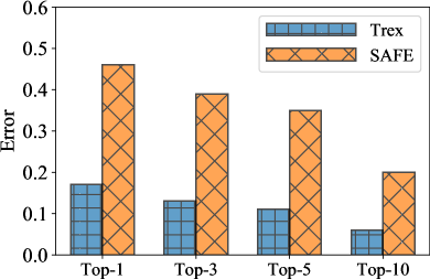
(a) Same architecture

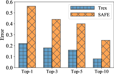
(b) Cross architecture

Figure 12: Top-1/3/5/10 error of Trex and SAFE in searching functions in firmware. (a) The query functions and the firmware are from same architecture (ARM). (b) The query functions are from x64 but the firmware are from ARM.

Figure 12 shows that Trex consistently outperforms SAFE, achieving 24.3% lower error rate on average. Moreover, as shown in Figure 12b, when the query functions are from x64 (the firmware binaries are from ARM), Trex outperforms SAFE by a greater margin, achieving 25.3% lower error rate in cross-architecture search.

TABLE VIII: Details of the real-world 180 firmware images we collected from DD-WRT.

Vendor	Model	ISA	Year	Vendor	Model	ISA	Year	Vendor	Model	ISA	Year
8devices	Carambola 2	MIPS	2020	8devices	Carambola 2 8MB	MIPS	2018	8devices	Lima	MIPS	2020
Actiontec	MI424WR	ARM	2019	Alfa	AIP-W502U	MIPS	2020	Alfa	SOLO48	MIPS	2020
Belkin	F5D8235-4	MIPS	2020	Buffalo	BHR-4GRV	MIPS	2020	Buffalo	WBMR-HP-G300H	MIPS	2020
Buffalo	WHR-1166D	MIPS	2020	Buffalo	WHR-300HP2	MIPS	2018	Buffalo	WHR-600D	MIPS	2018
Buffalo	WXR-1900DHP	ARM	2020	Buffalo	WZR-1166DHP	ARM	2020	Buffalo	WZR-600DHP2	ARM	2020
Buffalo	WZR-900DHP	ARM	2020	Buffalo	WZR-HP-G450H	MIPS	2020	Comfast	CF-E325N	MIPS	2020
Comfast	CF-E355AC	MIPS	2020	Comfast	CF-E380AC	MIPS	2020	Comfast	CF-WR650AC	MIPS	2020
Compex	WP546	MIPS	2020	Compex	WPE72	MIPS	2020	D-Link	DAP-2230	MIPS	2020
D-Link	DAP-2330	MIPS	2020	D-Link	DAP-2660	MIPS	2020	D-Link	DAP-3320	MIPS	2020
D-Link	DAP-3662	MIPS	2020	D-Link	DHP-1565 A1	MIPS	2020	D-Link	DIR-825 C1	MIPS	2020
D-Link	DIR-825 Rev.B	MIPS	2020	D-Link	DIR-835 A1	MIPS	2020	D-Link	DIR-859	MIPS	2020
D-Link	DIR-860L A1	ARM	2020	D-Link	DIR-860L B1	MIPS	2020	D-Link	DIR-862	MIPS	2020
D-Link	DIR-866	MIPS	2020	D-Link	DIR-868l Rev.A	ARM	2020	D-Link	DIR-868l Rev.B	ARM	2020
D-Link	DIR-868l Rev.C	ARM	2020	D-Link	DIR-869	MIPS	2020	D-Link	DIR-878 A1	MIPS	2020
D-Link	DIR-880l	ARM	2020	D-Link	DIR-882 A1	MIPS	2020	D-Link	DIR-885l	ARM	2020
D-Link	DIR-890l	ARM	2020	D-Link	DIR632A	MIPS	2020	GL.iNet	AR150	MIPS	2020
Gateworks	GW2382	ARM	2018	Gateworks	GW2388 16M	ARM	2018	Gateworks	GW2391	ARM	2018
Gateworks	Laguna GW2382	ARM	2020	Gateworks	Laguna GW2388 32M	ARM	2020	Gateworks	Laguna GW2391	ARM	2020
Gigaset	SX763	MIPS	2020	JJPlus	JA76PF	MIPS	2020	Linksys	E1700	MIPS	2020
Linksys	E2100L	MIPS	2020	Linksys	EA6350	ARM	2020	Linksys	EA6400	ARM	2020
Linksys	EA6500 v2	ARM	2020	Linksys	EA6700	ARM	2020	Linksys	EA6900	ARM	2020
Linksys	EA8500	ARM	2020	Linksys	RE7000	MIPS	2020	Linksys	WRT610N v1.0	MIPS	2020
NETGEAR	AC1450	ARM	2020	NETGEAR	EX6200	ARM	2018	NETGEAR	R6250	MIPS	2020
NETGEAR	R6300v2	ARM	2020	NETGEAR	R6400	ARM	2020	NETGEAR	R6700	ARM	2020
NETGEAR	R6700v3	ARM	2020	NETGEAR	R7000	ARM	2020	NETGEAR	R7000P	ARM	2020
NETGEAR	R7500v1	ARM	2020	NETGEAR	R7500v2	ARM	2020	NETGEAR	R7800	ARM	2020
NETGEAR	R8500	ARM	2020	NETGEAR	R8900	ARM	2020	NETGEAR	R9000	ARM	2020
NETGEAR	WG302v2	ARM	2020	NETGEAR	WNDR3700v4	MIPS	2020	NETGEAR	WNDR4300	MIPS	2020
NETGEAR	WNDR4500	MIPS	2020	NETGEAR	WNDR4500v2	MIPS	2020	NETGEAR	XR450	ARM	2020
NETGEAR	XR500	ARM	2020	NETGEAR	XR700	ARM	2020	Pronghorn	SBC	ARM	2020
Senao	ECB3500	MIPS	2020	Senao	ECB9750	MIPS	2019	Senao	EOC1650	MIPS	2020
Senao	EOC5510	MIPS	2020	Senao	EOC5610	MIPS	2020	Senao	EOC5611	MIPS	2020
Senao	NOP8670	ARM	2020	TP-Link	Archer A7 V5	MIPS	2020	TP-Link	Archer C1900	ARM	2020
TP-Link	Archer C25 V1	MIPS	2020	TP-Link	Archer C5 V1	MIPS	2020	TP-Link	Archer C7 V1	MIPS	2020
TP-Link	Archer C7 V2	MIPS	2020	TP-Link	Archer C7 V3	MIPS	2020	TP-Link	Archer C7 V4	MIPS	2020
TP-Link	Archer C8 V1	ARM	2020	TP-Link	Archer C9 V1	ARM	2020	TP-Link	Archer C9 V2	ARM	2020
TP-Link	Archer C9 V3	ARM	2020	TP-Link	Deco-M4	MIPS	2020	TP-Link	TL-WDR3600 V1	MIPS	2020
TP-Link	TL-WDR4300 V1	MIPS	2020	TP-Link	TL-WDR4310 V1	MIPS	2020	TP-Link	TL-WDR4900 V2	MIPS	2020
TP-Link	TL-WR1043N V5	MIPS	2020	TP-Link	TL-WR1043ND	MIPS	2020	TP-Link	TL-WR1043ND V2	MIPS	2020
TP-Link	TL-WR1043ND V4	MIPS	2020	TP-Link	TL-WR2543ND	MIPS	2020	TP-Link	TL-WR710N V1	MIPS	2020
TP-Link	TL-WR710N V2.1.0	MIPS	2020	TP-Link	TL-WR810N V1	MIPS	2020	TP-Link	TL-WR810N V2	MIPS	2020
TP-Link	TL-WR842N V1	MIPS	2020	TP-Link	TL-WR842N V2	MIPS	2020	TRENDnet	TEW-811DRU	ARM	2018
TRENDnet	TEW-812DRU V2	ARM	2018	TRENDnet	TEW-818DRU	ARM	2020	TRENDnet	TEW-828DRU	ARM	2020
Ubiquiti	AirGrid M2	MIPS	2020	Ubiquiti	AirGrid M5	MIPS	2020	Ubiquiti	AirGrid-M5-XW	MIPS	2020
Ubiquiti	AirRouter	MIPS	2020	Ubiquiti	AirRouter-HP	MIPS	2020	Ubiquiti	AirWire	MIPS	2020
Ubiquiti	BulletM2 HP	MIPS	2020	Ubiquiti	BulletM5 HP	MIPS	2020	Ubiquiti	LS SR71A	MIPS	2020
Ubiquiti	NanoBeam AC	MIPS	2020	Ubiquiti	NanoBeam M2 XW	MIPS	2020	Ubiquiti	NanoBeam M5 XW	MIPS	2020
Ubiquiti	NanoBridge M2	MIPS	2020	Ubiquiti	NanoBridge M2 XW	MIPS	2020	Ubiquiti	NanoBridge M3	MIPS	2020
Ubiquiti	NanoBridge M365	MIPS	2020	Ubiquiti	NanoBridge M5 XW	MIPS	2020	Ubiquiti	NanoBridge M900	MIPS	2020
Ubiquiti	NanoStation M2	MIPS	2020	Ubiquiti	NanoStation M3	MIPS	2020	Ubiquiti	NanoStation M365	MIPS	2020
Ubiquiti	Pico M5	MIPS	2020	Ubiquiti	Power AP N	MIPS	2020	Ubiquiti	PowerBeam M5 M400 XW	MIPS	2020
Ubiquiti	PowerBridge M10	MIPS	2020	Ubiquiti	PowerBridge M5	MIPS	2020	Ubiquiti	Rocket M2 Titanium XW	MIPS	2020
Ubiquiti	Rocket M2 XW	MIPS	2020	Ubiquiti	Rocket M5 Titanium XW	MIPS	2020	Ubiquiti	Rocket M5 X3 XW	MIPS	2020
Ubiquiti	Rocket M5 XW	MIPS	2020	Ubiquiti	RocketM2	MIPS	2020	Ubiquiti	RocketM3	MIPS	2020
Ubiquiti	RocketM365	MIPS	2020	Ubiquiti	RocketM5	MIPS	2020	Ubiquiti	RocketM900	MIPS	2020
Ubiquiti	RouterStation	MIPS	2020	Ubiquiti	RouterStation Pro	MIPS	2020	Ubiquiti	sunMax	MIPS	2020
Ubiquiti	UAP-AC-MESH	MIPS	2020	Ubiquiti	UAP-AC-PRO	MIPS	2020	Ubiquiti	UAP-LR	MIPS	2020
Ubiquiti	UAP-LR-v2	MIPS	2020	Ubiquiti	UAP-v2	MIPS	2020	Ubiquiti	locoM2	MIPS	2020
Ubiquiti	locoM2 XW	MIPS	2020	Ubiquiti	locoM5	MIPS	2020	Ubiquiti	locoM5 XW	MIPS	2020
Ubiquiti	locoM900	MIPS	2020	WiliGear	WBD-500	MIPS	2020	YunCore	XD3200	MIPS	2020

-D Probing Learned Execution Semantics

As discussed in Section II, training the model to predict masked micro-trace codes and values compels the model to learn execution semantics by concrete examples. It thus automates the extraction of the code’s dynamic features without manual effort. In this section, we study concrete code examples showing the potential hint in the code that the model likely leverages to predict the masked part.

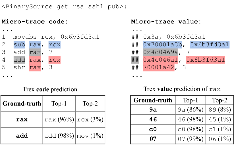
Figure 13: The partial micro-trace code and value sequence from function BinarySource_get_rsa_ssh1_pub in PuTTy-0.74 compiled to x64 with O0. We mask the register rax at line 3 and the opcode add at line 4. We also mask their corresponding micro-trace values (where opcode has only dummy values (8 ##s) as described in Section IV-B). We highlight the contextual hint in blue that Trex leverages to predict the masked rax and red that Trex uses to predict the masked add.

Predicting arithmetic instructions. Consider the example in Figure 13, which shows the function’s micro-trace (i.e., the dynamic value and assembly code). For ease of exposition, the format of micro-trace values (e.g., the value of opcode and constants) are not exactly the same as the actual format we handle, as described in Section IV-B. We mask the register rax and opcode add and their corresponding values in a sequence of arithmetic instructions.

To correctly predict the masked value 0x4c0469a of rax, the model should understand the approximate execution semantics of sub in line 2, which subtracts rax with rcx. It may also observe the value of rax at line 4, which exactly equals the result of adding rax with 7 at line 3. Therefore, we see the model predicts rax with 96% confidence and rcx with only 3%. It also predicts the value of rax correctly (right table). To correctly predict add at line 4, the model should observe that the rax at line 5 has the same exact value with the result of rax+rcx at line 4, so it predicts the opcode at line 4 to be add. As shown in Figure 13, our pretrained model predicts add with 98% confidence and mov with only 1%, which implies that the model approximately understands the execution semantics of add and mov so it predicts that add is much more likely.

Predicting stack operations. Consider the example in Figure 14. We mask the register and constant of the instruction in function epilogue – it increments the stack pointer rsp by 0x20 to deallocate the local variable stored on stack. To correctly predict the masked rsp and its value 0x8b4a3f, the model should observe the rsp is decremented (due to opcode sub) by 0x20 from 0x8b4a3f at line 3, which is part of the function prologue. Therefore, the model should understand the execution semantics of sub and basic syntax of function prologue and epilogue.

To predict the masked constant 0x20, the model should notice that line 3 decrements the stack pointer by 0x20, which is the size of local variables. As the model predicts 0x20 with 99% confidence, this implies the model likely learns patterns of function prologue and epilogue, including the context such as push ebp, pop ebp, etc. This observation indicates that our pretraining task assists in learning common function idiom (function calling convention) beyond execution semantics of individual instructions. Learning such knowledge can potentially help other tasks beyond function similarity, such as identifying function boundaries [62].

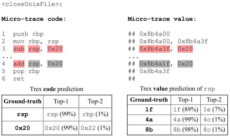
Figure 14: The partial code and micro-trace from function closeUnixFile in SQLite-3.34.0 compiled to x64 with O0. We mask the register rsp and constant 0x20 at line 4. We also mask their corresponding micro-trace values. We highlight the contextual hint in red that Trex leverages to predict the masked rsp and 0x20.

References

- [1] Hojjat Aghakhani, Fabio Gritti, Francesco Mecca, Martina Lindorfer, Stefano Ortolani, Davide Balzarotti, Giovanni Vigna, and Christopher Kruegel. When malware is packin’ heat; limits of machine learning classifiers based on static analysis features. In 2020 Network and Distributed Systems Security Symposium, 2020.
- [2] Miltiadis Allamanis, Earl T Barr, Premkumar Devanbu, and Charles Sutton. A survey of machine learning for big code and naturalness. ACM Computing Surveys, 2018.
- [3] Inc. Amazon Web Services. Open Distro for Elasticsearch. https://opendistro.github.io/for-elasticsearch/, 2020.
- [4] Dennis Andriesse, Asia Slowinska, and Herbert Bos. Compiler-agnostic function detection in binaries. In Proceedings of the 2017 IEEE European Symposium on Security and Privacy, 2017.
- [5] Thanassis Avgerinos, Sang Kil Cha, Alexandre Rebert, Edward J Schwartz, Maverick Woo, and David Brumley. Automatic exploit generation. Communications of the ACM, 2014.
- [6] Tiffany Bao, Jonathan Burket, Maverick Woo, Rafael Turner, and David Brumley. Byteweight: Learning to recognize functions in binary code. In 23rd USENIX Security Symposium, 2014.
- [7] Ulrich Bayer, Paolo Milani Comparetti, Clemens Hlauschek, Christopher Kruegel, and Engin Kirda. Scalable, behavior-based malware clustering. In 2009 Network and Distributed System Security Symposium, 2009.
- [8] Fabrice Bellard. QEMU, a fast and portable dynamic translator. In USENIX Annual Technical Conference, FREENIX Track, 2005.
- [9] James Bergstra and Yoshua Bengio. Random search for hyper-parameter optimization. Journal of Machine Learning Research, 2012.
- [10] Martial Bourquin, Andy King, and Edward Robbins. Binslayer: Accurate comparison of binary executables. In 2nd ACM SIGPLAN Program Protection and Reverse Engineering Workshop, 2013.
- [11] Leonid Boytsov and Bilegsaikhan Naidan. Engineering efficient and effective non-metric space library. In International Conference on Similarity Search and Applications, 2013.
- [12] David Brumley, Pongsin Poosankam, Dawn Song, and Jiang Zheng. Automatic patch-based exploit generation is possible: Techniques and implications. In 2008 IEEE Symposium on Security and Privacy, 2008.
- [13] Mahinthan Chandramohan, Yinxing Xue, Zhengzi Xu, Yang Liu, Chia Yuan Cho, and Hee Beng Kuan Tan. Bingo: Cross-architecture cross-os binary search. In 2016 24th ACM SIGSOFT International Symposium on Foundations of Software Engineering, 2016.
- [14] Daming D Chen, Maverick Woo, David Brumley, and Manuel Egele. Towards automated dynamic analysis for linux-based embedded firmware. In 2016 Network and Distributed System Security Symposium, 2016.
- [15] Ting Chen, Simon Kornblith, Mohammad Norouzi, and Geoffrey Hinton. A simple framework for contrastive learning of visual representations. arXiv preprint arXiv:2002.05709, 2020.
- [16] Zheng Leong Chua, Shiqi Shen, Prateek Saxena, and Zhenkai Liang. Neural nets can learn function type signatures from binaries. In Proceddings of the 26th USENIX Security Symposium, 2017.
- [17] Andrei Costin, Jonas Zaddach, Aurélien Francillon, and Davide Balzarotti. A large-scale analysis of the security of embedded firmwares. In 23rd USENIX Security Symposium, 2014.
- [18] Jonathan Crussell, Clint Gibler, and Hao Chen. Andarwin: Scalable detection of semantically similar android applications. In European Symposium on Research in Computer Security, 2013.
- [19] Yaniv David, Nimrod Partush, and Eran Yahav. Statistical similarity of binaries. ACM SIGPLAN Notices, 2016.
- [20] Yaniv David, Nimrod Partush, and Eran Yahav. Similarity of binaries through re-optimization. In 38th ACM SIGPLAN Conference on Programming Language Design and Implementation, 2017.
- [21] Yaniv David and Eran Yahav. Tracelet-based code search in executables. Acm Sigplan Notices, 2014.
- [22] Jacob Devlin, Ming-Wei Chang, Kenton Lee, and Kristina Toutanova. Bert: Pre-training of deep bidirectional transformers for language understanding. In 2019 Annual Conference of the North American Chapter of the Association for Computational Linguistics: Human Language Technologies, 2019.
- [23] devttys0. Binwalk - Firmware Analysis Tool. https://github.com/ReFirmLabs/binwalk.
- [24] Alessandro Di Federico, Mathias Payer, and Giovanni Agosta. rev.ng: A unified binary analysis framework to recover CFGs and function boundaries. In 26th International Conference on Compiler Construction, 2017.
- [25] Steven HH Ding, Benjamin CM Fung, and Philippe Charland. Asm2vec: Boosting static representation robustness for binary clone search against code obfuscation and compiler optimization. In 2019 IEEE Symposium on Security and Privacy, 2019.
- [26] Yue Duan, Xuezixiang Li, Jinghan Wang, and Heng Yin. Deepbindiff: Learning program-wide code representations for binary diffing. In 2020 Network and Distributed System Security Symposium, 2020.
- [27] Manuel Egele, Maverick Woo, Peter Chapman, and David Brumley. Blanket execution: Dynamic similarity testing for program binaries and components. In 23rd USENIX Security Symposium, 2014.
- [28] Sebastian Eschweiler, Khaled Yakdan, and Elmar Gerhards-Padilla. discovre: Efficient cross-architecture identification of bugs in binary code. In 2016 Network and Distributed System Security Symposium, 2016.
- [29] Mohammad Reza Farhadi, Benjamin CM Fung, Philippe Charland, and Mourad Debbabi. Binclone: Detecting code clones in malware. In International Conference on Software Security and Reliability, 2014.
- [30] Qian Feng, Rundong Zhou, Chengcheng Xu, Yao Cheng, Brian Testa, and Heng Yin. Scalable graph-based bug search for firmware images. In 2016 ACM SIGSAC Conference on Computer and Communications Security, 2016.
- [31] Cheng Fu, Huili Chen, Haolan Liu, Xinyun Chen, Yuandong Tian, Farinaz Koushanfar, and Jishen Zhao. Coda: An end-to-end neural program decompiler. In Advances in Neural Information Processing Systems, 2019.
- [32] Jian Gao, Xin Yang, Ying Fu, Yu Jiang, Heyuan Shi, and Jiaguang Sun. Vulseeker-pro: Enhanced semantic learning based binary vulnerability seeker with emulation. In 26th ACM Joint Meeting on European Software Engineering Conference and Symposium on the Foundations of Software Engineering, 2018.
- [33] Aristides Gionis, Piotr Indyk, Rajeev Motwani, et al. Similarity search in high dimensions via hashing. In Vldb, 1999.
- [34] Patrice Godefroid. Micro execution. In 36th International Conference on Software Engineering, 2014.
- [35] Sebastian Gottschall. Dd-wrt. https://dd-wrt.com/, 2005.
- [36] David Harris and Sarah Harris. Digital design and computer architecture. Morgan Kaufmann, 2010.
- [37] Kaiming He, Xiangyu Zhang, Shaoqing Ren, and Jian Sun. Deep residual learning for image recognition. In 2016 IEEE conference on computer vision and pattern recognition, 2016.
- [38] Dan Hendrycks and Kevin Gimpel. Gaussian error linear units (GELUs). arXiv preprint arXiv:1606.08415, 2016.
- [39] Yikun Hu, Yuanyuan Zhang, Juanru Li, and Dawu Gu. Binary code clone detection across architectures and compiling configurations. In IEEE/ACM International Conference on Program Comprehension, 2017.
- [40] He Huang, Amr M Youssef, and Mourad Debbabi. Binsequence: Fast, accurate and scalable binary code reuse detection. In 2017 ACM on Asia Conference on Computer and Communications Security, 2017.
- [41] Jiyong Jang, Maverick Woo, and David Brumley. Towards automatic software lineage inference. In 22nd USENIX Security Symposium, 2013.
- [42] Lingxiao Jiang and Zhendong Su. Automatic mining of functionally equivalent code fragments via random testing. In 18th International Symposium on Software Testing and Analysis, 2009.
- [43] Roberto Jordaney, Kumar Sharad, Santanu K Dash, Zhi Wang, Davide Papini, Ilia Nouretdinov, and Lorenzo Cavallaro. Transcend: Detecting concept drift in malware classification models. In 26th USENIX Security Symposium (USENIX Security 17), 2017.
- [44] Mandar Joshi, Danqi Chen, Yinhan Liu, Daniel S Weld, Luke Zettlemoyer, and Omer Levy. Spanbert: Improving pre-training by representing and predicting spans. Transactions of the Association for Computational Linguistics, 2020.
- [45] Alexandros Kapravelos, Yan Shoshitaishvili, Marco Cova, Christopher Kruegel, and Giovanni Vigna. Revolver: An automated approach to the detection of evasive web-based malware. In 22nd USENIX Security Symposium, 2013.
- [46] Deborah S Katz, Jason Ruchti, and Eric Schulte. Using recurrent neural networks for decompilation. In 25th IEEE International Conference on Software Analysis, Evolution and Reengineering, 2018.
- [47] Wei Ming Khoo, Alan Mycroft, and Ross Anderson. Rendezvous: A search engine for binary code. In 10th Working Conference on Mining Software Repositories, 2013.
- [48] Solomon Kullback and Richard A Leibler. On information and sufficiency. The annals of mathematical statistics, 22(1):79–86, 1951.
- [49] Lannan Luo, Jiang Ming, Dinghao Wu, Peng Liu, and Sencun Zhu. Semantics-based obfuscation-resilient binary code similarity comparison with applications to software plagiarism detection. In ACM SIGSOFT International Symposium on Foundations of Software Engineering, 2014.
- [50] Luca Massarelli, Giuseppe Antonio Di Luna, Fabio Petroni, Roberto Baldoni, and Leonardo Querzoni. Safe: Self-attentive function embeddings for binary similarity. In International Conference on Detection of Intrusions and Malware, and Vulnerability Assessment, 2019.
- [51] Derrick McKee, Nathan Burow, and Mathias Payer. Software ethology: An accurate and resilient semantic binary analysis framework. arXiv preprint arXiv:1906.02928, 2019.
- [52] Jiang Ming, Meng Pan, and Debin Gao. ibinhunt: Binary hunting with inter-procedural control flow. In International Conference on Information Security and Cryptology, 2012.
- [53] Jiang Ming, Dongpeng Xu, Yufei Jiang, and Dinghao Wu. Binsim: Trace-based semantic binary diffing via system call sliced segment equivalence checking. In 26th USENIX Security Symposium, 2017.
- [54] Ginger Myles and Christian Collberg. K-gram based software birthmarks. In 2005 ACM symposium on Applied computing, 2005.
- [55] Myle Ott, Sergey Edunov, Alexei Baevski, Angela Fan, Sam Gross, Nathan Ng, David Grangier, and Michael Auli. fairseq: A fast, extensible toolkit for sequence modeling. In 2019 Annual Conference of the North American Chapter of the Association for Computational Linguistics: Human Language Technologies: Demonstrations, 2019.
- [56] OWASP. Top 10 web application security risks. https://owasp.org/www-project-top-ten/, 2010.
- [57] Fabio Pagani, Matteo Dell’Amico, and Davide Balzarotti. Beyond precision and recall: understanding uses (and misuses) of similarity hashes in binary analysis. In 8th ACM Conference on Data and Application Security and Privacy, 2018.
- [58] Sagar Parihar, Ziyaan Dadachanji, Praveen Kumar Singh, Rajdeep Das, Amey Karkare, and Arnab Bhattacharya. Automatic grading and feedback using program repair for introductory programming courses. In 2017 ACM Conference on Innovation and Technology in Computer Science Education, 2017.
- [59] Adam Paszke, Sam Gross, Francisco Massa, Adam Lerer, James Bradbury, Gregory Chanan, Trevor Killeen, Zeming Lin, Natalia Gimelshein, Luca Antiga, et al. Pytorch: An imperative style, high-performance deep learning library. In Advances in neural information processing systems, 2019.
- [60] James Patrick-Evans, Lorenzo Cavallaro, and Johannes Kinder. Probabilistic naming of functions in stripped binaries. In Annual Computer Security Applications Conference, 2020.
- [61] Mathias Payer, Stephen Crane, Per Larsen, Stefan Brunthaler, Richard Wartell, and Michael Franz. Similarity-based matching meets malware diversity. arXiv preprint arXiv:1409.7760, 2014.
- [62] Kexin Pei, Jonas Guan, David Williams King, Junfeng Yang, and Suman Jana. Xda: Accurate, robust disassembly with transfer learning. In Proceedings of the 2021 Network and Distributed System Security Symposium (NDSS), 2021.
- [63] Fei Peng, Zhui Deng, Xiangyu Zhang, Dongyan Xu, Zhiqiang Lin, and Zhendong Su. X-force: force-executing binary programs for security applications. In 23rd USENIX Security Symposium, 2014.
- [64] Jannik Pewny, Behrad Garmany, Robert Gawlik, Christian Rossow, and Thorsten Holz. Cross-architecture bug search in binary executables. In 2016 IEEE Symposium on Security and Privacy, 2016.
- [65] Jannik Pewny, Felix Schuster, Lukas Bernhard, Thorsten Holz, and Christian Rossow. Leveraging semantic signatures for bug search in binary programs. In 30th Annual Computer Security Applications Conference, 2014.
- [66] NGUYEN Anh Quynh and DANG Hoang Vu. Unicorn: Next generation cpu emulator framework. BlackHat USA, 2015.
- [67] Anand Rajaraman and Jeffrey David Ullman. Mining of massive datasets. Cambridge University Press, 2011.
- [68] Veselin Raychev, Martin Vechev, and Eran Yahav. Code completion with statistical language models. In 35th ACM Conference on Programming Language Design and Implementation, 2014.
- [69] Konrad Rieck, Philipp Trinius, Carsten Willems, and Thorsten Holz. Automatic analysis of malware behavior using machine learning. Journal of Computer Security, 2011.
- [70] Nikunj Saunshi, Orestis Plevrakis, Sanjeev Arora, Mikhail Khodak, and Hrishikesh Khandeparkar. A theoretical analysis of contrastive unsupervised representation learning. In International Conference on Machine Learning, 2019.
- [71] Zhan Shi, Kevin Swersky, Daniel Tarlow, Parthasarathy Ranganathan, and Milad Hashemi. Learning execution through neural code fusion. In 2019 International Conference on Learning Representations, 2019.
- [72] Eui Chul Richard Shin, Dawn Song, and Reza Moazzezi. Recognizing functions in binaries with neural networks. In 24th USENIX Security Symposium, 2015.
- [73] VMPROTECT SOFTWARE. VMProtect Software Protection. http://vmpsoft.com.
- [74] Xabier Ugarte-Pedrero, Davide Balzarotti, Igor Santos, and Pablo G Bringas. SoK: Deep packer inspection: A longitudinal study of the complexity of run-time packers. In 2015 IEEE Symposium on Security and Privacy, 2015.
- [75] Ashish Vaswani, Noam Shazeer, Niki Parmar, Jakob Uszkoreit, Llion Jones, Aidan N Gomez, Łukasz Kaiser, and Illia Polosukhin. Attention is all you need. In 2017 Advances in Neural Information Processing Systems, 2017.
- [76] Shuai Wang, Pei Wang, and Dinghao Wu. Semantics-aware machine learning for function recognition in binary code. In 2017 IEEE International Conference on Software Maintenance and Evolution, 2017.
- [77] Xiaojun Xu, Chang Liu, Qian Feng, Heng Yin, Le Song, and Dawn Song. Neural network-based graph embedding for cross-platform binary code similarity detection. In 2017 ACM SIGSAC Conference on Computer and Communications Security, 2017.
- [78] Naville Zhang. Hikari – an improvement over Obfuscator-LLVM. https://github.com/HikariObfuscator/Hikari, 2017.
- [79] Zynamics. BinDiff. https://www.zynamics.com/bindiff.html, 2019.