Imperial/TP/2020/JG/05

Accelerating Black Holes and Spinning Spindles

Pietro Ferrero^a, Jerome P. Gauntlett^b, Juan Manuel Pérez Ipiña^a,

Dario Martelli^c,d,e and James Sparks^a

${}^{\,\mathrm{a}}$Mathematical Institute, University of Oxford,
Andrew Wiles Building, Radcliffe Observatory Quarter,
Woodstock Road, Oxford, OX2 6GG, U.K.

^bBlackett Laboratory, Imperial College,
Prince Consort Rd., London, SW7 2AZ, U.K.

^cDipartimento di Matematica “Giuseppe Peano”, Università di Torino,
Via Carlo Alberto 10, 10123 Torino, Italy

^dINFN, Sezione di Torino & ^eArnold–Regge Center,
Via Pietro Giuria 1, 10125 Torino, Italy

We study solutions in the Plebański–Demiański family which describe an accelerating, rotating and dyonically charged black hole in $AdS_{4}$. These are solutions of $D=4$ Einstein-Maxwell theory with a negative cosmological constant and hence minimal $D=4$ gauged supergravity. It is well known that when the acceleration is non-vanishing the $D=4$ black hole metrics have conical singularities. By uplifting the solutions to $D=11$ supergravity using a regular Sasaki-Einstein $7$-manifold, $SE_{7}$, we show how the free parameters can be chosen to eliminate the conical singularities. Topologically, the $D=11$ solutions incorporate an $SE_{7}$ fibration over a two-dimensional weighted projective space, $\mathbb{WCP}^{1}_{[n_{-},n_{+}]}$, also known as a spindle, which is labelled by two integers that determine the conical singularities of the $D=4$ metrics. We also discuss the supersymmetric and extremal limit and show that the near horizon limit gives rise to a new family of regular supersymmetric $AdS_{2}\times Y_{9}$ solutions of $D=11$ supergravity, which generalise a known family by the addition of a rotation parameter. We calculate the entropy of these black holes and argue that it should be possible to derive this from certain ${\cal N}=2$, $d=3$ quiver gauge theories compactified on a spinning spindle with appropriate magnetic flux.

1 Introduction

The $C$-metrics of $D=4$ Einstein-Maxwell theory [2] describe two charged black holes undergoing uniform acceleration. The force for the acceleration is provided by a conical angle excess (a strut) between the two black holes, a conical angle deficit (a string) attached to the black holes and extending out to infinity, or a combination of the two. By extending the model to include additional matter fields that allow for cosmic strings, the conical singularity can be smoothed out by having two cosmic strings pull the black holes apart [3, 4]. Another approach for removing the conical singularities, in the case of electrically or magnetically charged black holes, is provided by the Ernst metric in which the black holes are being accelerated by a background electric or magnetic field, respectively [5].

Generalizations of the Ernst metric were found for Einstein-Maxwell-dilaton gravity in [6]. For the particular case associated with $D=5$ Kaluza-Klein theory it was shown in [7] that the accelerating $D=4$ extremal, magnetically charged black hole solutions can be obtained by a dimensional reduction of a double Wick rotation of the $D=5$ generalization of the Kerr solution [8]. Recall the extremal magnetically charged black holes in Kaluza-Klein theory are Kaluza-Klein monopoles [9, 10], which are in fact naked singularities from the four-dimensional point of view. A key ingredient in the construction of [7] is that the Kaluza-Klein circle action associated with the reduction has two fixed points which precisely correspond to a Kaluza-Klein monopole, anti-monopole pair.

In this paper we provide a new way of desingularising the conical deficits for a specific class of accelerating, rotating and dyonically charged black holes in $AdS_{4}$, by embedding them in $D=11$ supergravity. We study the Plebański–Demiański (PD) solutions [11] of $D=4$ Einstein-Maxwell theory, generalising the $C$-metrics of [2], which in particular allow for a cosmological constant, which we take to be negative. Such accelerating $AdS_{4}$ black holes have been extensively studied (e.g. [12, 13, 14]) and here we will only be interested in the case of small acceleration for which there is just a single black hole. From a $D=4$ perspective we will consider a single accelerating black hole with a two-dimensional horizon given by a “spindle”, a weighted projective space, $\mathbb{WCP}^{1}_{[n_{-},n_{+}]}$, which is topologically a sphere with conical deficits at both poles specified by $n_{\pm}\in\mathbb{N}$, which stretch out to the $AdS_{4}$ boundary. The net acceleration of the black hole is due to the mismatch of the conical deficits on either side of the black hole. Interestingly, the same mismatch also leads to a non-zero magnetic flux though the horizon, given by $G_{(4)}Q_{m}=\tfrac{n_{-}-n_{+}}{4n_{+}n_{-}}$.

We can embed these solutions in $D=11$ supergravity, locally, using an arbitrary seven-dimensional Sasaki-Einstein manifold $SE_{7}$. Indeed it has been shown [15] that there is a consistent Kaluza-Klein truncation of $D=11$ supergravity on any $SE_{7}$ down to minimal gauged supergravity in $D=4$, whose bosonic content is Einstein-Maxwell theory (with a negative cosmological constant). By definition, this means that any solution of $D=4$ Einstein-Maxwell theory can be uplifted on an arbitrary $SE_{7}$ manifold to obtain a solution of $D=11$ supergravity. Furthermore, if the $D=4$ solution preserves supersymmetry then so does the uplifted solution. For example the vacuum $AdS_{4}$ solution, which preserves all of the $D=4$ supersymmetry, uplifts to the $AdS_{4}\times SE_{7}$ solution which, in general, preserves 1/4 of the supersymmetry and is dual to an $\mathcal{N}=2$ supersymmetric conformal field theory (SCFT) in $d=3$.

In our construction it is only the regular class of $SE_{7}$ that play a role in obtaining smooth $D=11$ solutions. These have the property that the $SE_{7}$ manifold is a circle bundle over $KE_{6}$, a six-dimensional Kähler-Einstein manifold with positive curvature. It will also be important to recall that this includes the generic class where the circle bundle is the canonical bundle of the Kähler-Einstein manifold, but it is also possible, depending on the choice of $KE_{6}$, to enlarge the period of the circle to get other Sasaki-Einstein manifolds. The simplest example is for the case of $\mathbb{CP}^{3}$: for this case $S^{7}/\mathbb{Z}_{4}$ is the canonical circle bundle over $\mathbb{CP}^{3}$ and is a smooth Sasaki-Einstein manifold, but so too are $S^{7}/\mathbb{Z}_{2}$ and $S^{7}$.

After uplifting the PD black hole solutions with horizon $\mathbb{WCP}^{1}_{[n_{-},n_{+}]}$ on a regular $SE_{7}$ we will show, somewhat miraculously, that by choosing the parameters in the PD metric appropriately, the $D=11$ solution is free from any conical deficit singularities. Importantly, precisely which regular Sasaki-Einstein manifold one can uplift upon depends on the integers $n_{\pm}\in\mathbb{N}$. For example, for the case of $\mathbb{CP}^{3}$, for given $n_{\pm}\in\mathbb{N}$ we can uplift on precisely one of the three cases $S^{7}$, $S^{7}/\mathbb{Z}_{2}$ or $S^{7}/\mathbb{Z}_{4}$. It is also important to note that for the Kaluza-Klein reduction on the $SE_{7}$ the fibred circle action does not have any fixed points and hence there are no Kaluza-Klein monopoles as in the construction of [7]. On the other hand, the circle action is not free and this leads to the conical deficits of the spindle $\mathbb{WCP}^{1}_{[n_{-},n_{+}]}$.

Of particular interest is that our construction also includes accelerating black holes that preserve supersymmetry, as considered in a general context in [16], and, moreover, have regular extremal horizons. From the $D=4$ perspective, the near horizon limit of these supersymmetric, extremal, rotating black holes are of the form $AdS_{2}\times\mathbb{WCP}^{1}_{[n_{-},n_{+}]}$, with non-vanishing magnetic flux through the horizon $\mathbb{WCP}^{1}_{[n_{-},n_{+}]}$. The way that supersymmetry is preserved for these $AdS_{2}$ solutions is non-standard: the magnetic flux is not describing a topological twist [17, 18], and the Killing spinors are then correspondingly not simply constant, even when the rotation is turned off; indeed, they are sections of non-trivial bundles over the spindle $\mathbb{WCP}^{1}_{[n_{-},n_{+}]}$. The uplifted supersymmetric $D=11$ solutions have a near horizon limit of the form $AdS_{2}\times Y_{9}$. In the special case that we set the rotation parameter of the PD metrics to zero, we find an $AdS_{2}\times Y_{9}$ geometry in the general class of [19], where $Y_{9}$ is a nine-dimensional Gauntlett-Kim (GK) geometry [20]. In fact, remarkably, when the rotation parameter vanishes we find exactly the same class of supersymmetric $AdS_{2}\times Y_{9}$ solutions first constructed in [1] from a quite different perspective. When the rotation parameter of the PD metrics is non-zero we find a new class of supersymmetric $AdS_{2}\times Y_{9}$ solutions that lie outside the class considered in [19], and generalize those of [1] with an extra rotation parameter.

We calculate the entropy $S_{BH}$ for the PD black hole solutions. In particular, for the “supersymmetric spinning spindles” that in addition have extremal horizons, we find

$$S_{BH}=\frac{\pi}{G_{(4)}}\frac{J}{Q_{e}}=\frac{\pi}{G_{(4)}}\frac{\sqrt{2}\sqrt{n_{-}^{2}+n_{+}^{2}+8n_{-}^{2}n_{+}^{2}(G_{(4)}Q_{e})^{2}}-(n_{-}+n_{+})}{4n_{-}n_{+}}\,,$$ (1.1)

where $J$ is the angular momentum of the black hole, and $Q_{e}$ is its electric charge. Notice this gives a relation between $J$ and $Q_{e}$ for extremal solutions. We also note that with non-zero acceleration, we can still have supersymmetric extremal black holes with $J=Q_{e}=0$; for these black holes the second expression in (1.1) is the valid expression. We also recall that $\frac{\pi}{2G_{(4)}}=\mathcal{F}_{S^{3}}$ is the free energy of the $d=3$ SCFT dual to the $AdS_{4}\times SE_{7}$ solution.

We define the angular momentum $J$ of the black hole, appearing in (1.1), to be a conserved quantity that can be equally evaluated either at the conformal boundary or at the black hole horizon (see e.g. [22]). As a consequence it is a type of Page charge that depends on the gauge used for the gauge field. However, there is a different natural angular momentum defined in the near horizon limit which has a gauge field that is invariant under the $AdS_{2}$ symmetries, that we denote $J_{AdS_{2}}$. We find

$$J_{AdS_{2}}-J=\frac{Q_{e}}{4}\chi(\Sigma)\,,$$ (1.2)

where $\chi(\Sigma)=\frac{n_{-}+n_{+}}{n_{+}n_{-}}$ is the Euler number of the spindle horizon $\Sigma=\mathbb{WCP}^{1}_{[n_{-},n_{+}]}$.

It would be very interesting to be able to derive this entropy from the $d=3$ SCFT dual to the corresponding $AdS_{4}\times SE_{7}$ vacuum solution. In the context of the topological twist, there has been considerable progress in obtaining such derivations for supersymmetric $AdS_{4}$ black holes with magnetic flux through a Riemann surface horizon using the principle of $I$-extremization [23, 24, 25, 26, 27, 28, 29, 30]. The relevant black hole solutions approach $AdS_{4}\times SE_{7}$ in the UV and $AdS_{2}\times Y_{9}$ in the near horizon, with $Y_{9}$ a $SE_{7}$ fibration over the Riemann surface, $\Sigma_{g}$. The black hole entropy can be obtained from the $d=3$ field theory by extremizing a certain twisted topological index [31] associated with the $d=3$ SCFT compactified on $\Sigma_{g}$. This index can be calculated using localization techniques and then evaluated in the large $N$ limit for many different examples [32, 33]. A geometric dual of $I$-extremization was proposed in [34, 35] and later shown to agree with the $I$-extremization procedure in field theory for infinite classes of examples of such $AdS_{2}\times Y_{9}$ solutions in [27, 28, 29, 30].

The family of black holes that we consider includes the well-known Kerr-Newman-AdS spacetime [36] in the non-accelerating case, whose Bogomolnyi-Prasad-Somerfeld (BPS), i.e. supersymmetric, and extremal limits have been extensively discussed both from the gravitational, as well as from the dual field theory points of view, see e.g. [37, 38, 39, 40] and [41, 42], respectively. Interestingly, the entropy of the BPS and extremal Kerr-Newman-AdS black hole can be immediately recovered from (1.1) by setting $n_{+}=n_{-}=1$. In addition, the expression (1.2) is also valid for the Kerr-Newman-AdS black holes, a point that seems to have been overlooked in the literature.

The results of this paper lead to the challenge of recovering the entropy of the rotating and accelerating black hole, by evaluating a suitable index. This index will be an appropriately defined localized partition function of the dual $d=3$ SCFT compactified on $S^{1}\times\mathbb{WCP}^{1}_{[n_{-},n_{+}]}$, with electric flux and magnetic flux through $\mathbb{WCP}^{1}_{[n_{-},n_{+}]}$, and with additional rotation. There are a number of subtleties related to this computation, which will need to be further developed in future work. Here we will make a number of particularly interesting observations concerning the BPS extremal black holes with acceleration but without rotation or electric charge i.e. $J=Q_{e}=0$. One feature is that these solutions have an acceleration horizon that intersects the conformal boundary, effectively dividing the spindle in half. Moreover, we find that the Killing spinor on this conformal boundary is given by a topological twist, so that the spinor is constant, but it is a different constant spinor on each half of the space! We also explain how these unusual features are “regulated” by keeping, for example, supersymmetry but relaxing the extremality condition (although this class with $J=0$ then has a naked singularity in the bulk).

The plan of the rest of this paper is as follows. In section 2 we briefly review $D=4$ minimal gauged supergravity, and its uplift to $D=11$ supergravity on Sasaki-Einstein seven-manifolds. Section 3 introduces the class of Plebański–Demiański solutions of interest, showing that the parameters can be chosen so that the black hole horizon is topologically a spindle, $\mathbb{WCP}^{1}_{[n_{-},n_{+}]}$. In section 4 we show that on uplifting to $D=11$ supergravity the PD solutions become completely smooth, with properly quantized flux. Supersymmetric and extremal solutions are studied in section 5, where we focus on the near horizon $AdS_{2}$ geometries and associated Killing spinors. In section 6 we discuss some global properties of the accelerating but non-rotating extremal supersymmetric black hole, discussing the conformal boundary and the acceleration horizon. We conclude with a discussion of open problems in section 7.

We have also included a number of appendices. Appendix A has some general comments on circle bundles over spindles. Appendix B briefly discusses some aspects of the well-known non-accelerating class of Kerr-Newman-AdS black holes. Appendix C contains some technical details concerning the near horizon limit, while appendix D shows that the resulting supersymmetric $AdS_{2}\times Y_{9}$ solutions generalize those of [1] by the addition of an angular momentum parameter. In appendix E we discuss how we define the angular momentum of the black holes, clarify various aspects of the gauge dependence and also derive (1.2). Appendix F discusses conventions for Killing spinors while appendix G contains some details of how to obtain the bulk Killing spinor, as well as how to obtain the associated Killing spinor on the three-dimensional conformal boundary.

2 General setting

We will be interested in solutions of $D=4$ Einstein-Maxwell theory with action given by

$$S=\frac{1}{16\pi G_{(4)}}\int d^{4}x\sqrt{-g}\big{(}R+6-F^{2}\big{)}\,,$$ (2.1)

with $F=dA$. This is the action for the bosonic fields of $D=4$, $\mathcal{N}=2$ minimal gauged supergravity. A solution to the equations of motion will preserve supersymmetry provided that it admits appropriate Killing spinors which we define later. Note that we have performed a scaling to set the cosmological constant as $\Lambda=-3$ so that a unit radius $AdS_{4}$ vacuum solution, with vanishing gauge field, solves the equations of motion. This vacuum solution preserves all of the $D=4$ supersymmetry.

Any (supersymmetric) solution of this theory automatically uplifts to a (supersymmetric) solution of $D=11$ supergravity on an arbitrary Sasaki-Einstein 7-manifold, $SE_{7}$ [15]. The general uplifting ansatz is

$$ds^{2}_{11} =L^{2}\left[\tfrac{1}{4}ds^{2}_{4}+\left(\eta+\tfrac{1}{2}A\right)^{2}+ds^{2}_{T}\right]\,,$$

$$G =L^{3}\left[\tfrac{3}{8}\mathrm{vol}_{4}-\tfrac{1}{2}*_{4}F\wedge J\right]\,,$$ (2.2)

where $L>0$ is a constant which is eventually fixed by flux quantization. Here $\eta$ is the contact one-form of the Sasaki-Einstein manifold, with transverse Kähler two-form $J$ and associated transverse metric $ds^{2}_{T}$, with $d\eta=2J$. The vacuum $AdS_{4}$ solution, with $\mathrm{d}s^{2}_{4}$ a unit radius $AdS_{4}$ and $A=0$, uplifts to the supersymmetric $AdS_{4}\times SE_{7}$ solution, dual to an $\mathcal{N}=2$ SCFT in $d=3$. For later use we note that

$$*_{11}G=L^{6}\Big{[}J^{3}\wedge(\eta+\tfrac{1}{2}A)+\frac{1}{2^{4}}F\wedge J^{2}\wedge(\eta+\tfrac{1}{2}A)\Big{]}\,.$$ (2.3)

In this paper we will be interested in the case that the Sasaki-Einstein manifold is in the regular class, for which $ds^{2}_{T}=ds^{2}_{KE_{6}}$ is a metric on $KE_{6}$, a Kähler-Einstein manifold. Necessarily, $KE_{6}$ has positive curvature and $ds^{2}_{T}$ is normalized so that $Ric(KE_{6})=8g(KE_{6})$ and hence $\rho=8J$, where $\rho$ is the Ricci form. Introducing local coordinates we can write

$$\eta=\tfrac{1}{4}d\psi+\sigma\,,\qquad d\sigma=2J\,.$$ (2.4)

The Sasaki-Einstein manifold admits a Killing spinor which has charge $1/2$ under $\partial_{\psi}$ (see appendix F). That is, in a frame invariant under $\partial_{\psi}$ there is an explicit phase $\mathrm{e}^{\mathrm{i}\psi/2}$ in the spinor. This gives rise to a phase $\mathrm{e}^{\mathrm{i}\psi}$ in the holomorphic $(4,0)$-form on the cone over the $SE_{7}$, which is a bilinear in the Killing spinor.

In the sequel it will be important to recall that the $KE_{6}$ has a Fano index $I\in\mathbb{N}$. If $\mathcal{L}$ is the canonical line bundle over the $KE_{6}$ then $I$ is the largest integer for which there is a line bundle $\mathcal{N}$ with $\mathcal{L}=\mathcal{N}^{I}$, i.e. we are able to take the $I$th root of the canonical bundle. In general we may then take the period of $\psi$ to be

$$\Delta\psi=\frac{2\pi I}{k}\,,$$ (2.5)

where $k$ is a positive integer that divides $I$. The fundamental group is then $\pi_{1}(SE_{7})\cong\mathbb{Z}_{k}$, so that in particular when $k=1$ the resulting manifold is simply-connected. For example, if $KE_{6}=\mathbb{CP}^{3}$, then $I=4$ and the associated $SE_{7}$ manifolds with $k=1,2$ and $4$ are respectively $S^{7}$, $S^{7}/\mathbb{Z}_{2}$ and $S^{7}/\mathbb{Z}_{4}$. Note that $I/k\in\mathbb{N}$ ensures that the Killing spinor and holomorphic $(4,0)$-form mentioned above are well-defined. Some other well-known examples of regular $SE_{7}$ are summarized in Table 1, with the associated values of $I$ (see e.g. Theorem 3.1 of [43].)

Another integer quantity associated with the $KE_{6}$ that will frequently appear is defined by

$$M\equiv\int_{KE_{6}}\left(\frac{\rho}{2\pi}\right)^{3}=\int_{KE_{6}}c_{1}^{3}\,,$$ (2.6)

where $\rho$ is the Ricci form for the $KE_{6}$. Values of $M$ for examples of $SE_{7}$ can also be found in Table 1. We note that the volume of the $KE_{6}$ and the $SE_{7}$ can be expressed in terms of $M$ as follows

$$\mathrm{vol}(KE_{6})=\frac{\pi^{3}M}{3\times 2^{7}}~{},\qquad\mathrm{vol}(SE_{7})=\frac{\pi^{4}MI}{3\times 2^{8}k}\,.$$ (2.7)

Our conventions for $D=11$ supergravity are as in e.g. [44, 45]. We define $N_{SE}>0$ to be the quantized flux through the $SE_{7}$ manifold:

$$N_{SE}\equiv\frac{1}{(2\pi\ell_{p})^{6}}\int_{SE_{7}}*_{11}G=\frac{3L^{6}\mathrm{vol}(SE_{7})}{\pi^{6}2^{5}\ell_{p}^{6}}\,.$$ (2.8)

Here $\ell_{p}$ is the $D=11$ Planck length with the $D=11$ Newton’s constant defined by $1/(16\pi G_{(11)})=1/(2\pi)^{8}\ell_{p}^{9}$. Carrying out the dimensional reduction to $D=4$ we can now express the $D=4$ Newton constant in the following useful form

$$\frac{1}{G_{(4)}}=\frac{2^{3/2}\pi^{2}}{3^{3/2}\mathrm{vol}(SE_{7})^{1/2}}{N_{SE_{7}}^{3/2}}=\frac{2^{11/2}k^{1/2}}{3M^{1/2}I^{1/2}}N_{SE_{7}}^{3/2}\,.$$ (2.9)

We also recall that the free energy of the $d=3$ SCFT dual to the $AdS_{4}\times SE_{7}$ solution is given by

$$\mathcal{F}_{S^{3}}=\frac{\pi}{2G_{(4)}}\,.$$ (2.10)

$KE_{6}$	$I$	$M$	$SE_{7}$ (with $k=1$)
$\mathbb{CP}^{3}$	4	$2^{6}$	$S^{7}$
$\mathbb{CP}^{1}\times\mathbb{CP}^{1}\times\mathbb{CP}^{1}$	2	$2^{4}\times 3$	$Q^{1,1,1}$
$\mathbb{CP}^{2}\times\mathbb{CP}^{1}$	1	$2\times 3^{3}$	$M^{3,2}$
$SU(3)/T^{2}$	2	$2^{4}\times 3$	$N^{1,1}$
$Gr_{5,2}$	3	$2\times 3^{3}$	$V_{5,2}$
$dP_{n}\times\mathbb{CP}^{1}$	1	$6\times(9-n)$	$\star$

Table 1: Some examples of simply-connected ($k=1$) $SE_{7}$ manifolds obtained as circle bundles over a $KE_{6}$ manifold. The integer $I$ is the Fano index for the $KE_{6}$ and $M$ is defined in (2.6). Note that $dP_{n}$ are del-Pezzo surfaces with $n=3,\dots,8$ and the associated $SE_{7}$ do not have a name.

3 $AdS_{4}$ PD black holes in $D=4$

We start with a sub-class of the class of Plebański–Demiański (PD) solutions [11] of Einstein-Maxwell theory, as presented in [46]. The metric is given by

$$ds^{2} =\frac{1}{H^{2}}\bigg{\{}-\frac{Q}{\Sigma}\big{[}dt-a\sin^{2}\theta\,d\phi\big{]}^{2}+\frac{\Sigma}{Q}\,dr^{2}+\frac{\Sigma}{P}d\theta^{2}$$

$$\qquad\qquad\qquad\qquad+\frac{P}{\Sigma}\sin^{2}\theta\big{[}adt-(r^{2}+a^{2})d\phi\big{]}^{2}\bigg{\}},$$ (3.1)

where

$$H =1-\alpha\,r\cos\theta\,,$$

$$\Sigma =r^{2}+a^{2}\cos^{2}\theta\,,$$

$$P =1-2\alpha m\cos\theta+\Big{(}\alpha^{2}(a^{2}+e^{2}+g^{2})-a^{2}\Big{)}\cos^{2}\theta\,,$$

$$Q =\Big{(}r^{2}-2mr+a^{2}+e^{2}+g^{2}\Big{)}(1-\alpha^{2}r^{2})+(a^{2}+r^{2})r^{2}\,,$$ (3.2)

and we note that $P=P(\theta)$ and $Q=Q(r)$ while $H$ and $\Sigma$ depend on both $r$ and $\theta$. The gauge field is given by

$$A=-e\frac{r}{\Sigma}(dt-a\sin^{2}\theta d\phi)+g\frac{\cos\theta}{\Sigma}(adt-(r^{2}+a^{2})d\phi)\,.$$ (3.3)

The solution depends on five free parameters $m,e,g,a$ and $\alpha$, which we can loosely associate with mass, electric charge, magnetic charge, rotation and acceleration, respectively. We note that we have set a possible NUT (Newman-Unti-Tamburino) parameter in the PD metrics to zero, since we want to avoid closed timelike curves. We have fixed the cosmological constant to be $\Lambda=-3$, as in (2.1), and finally we note that we have changed the sign of $g$ compared with [46].

We will assume $m>0$. Note that there are various coordinate changes $\theta\to\pi-\theta$, $t\to-t$, $\phi\to-\phi$ as well as $A\to-A$, which change the signs of the pairs $(\alpha,g)$, $(a,e)$, $(a,g)$ and $(e,g)$, respectively. If $\alpha=0$ we can thus choose $e,g,a\geq 0$ without loss of generality. If $\alpha\neq 0$ we can choose $m,\alpha>0$ and $e,g\geq 0$ with either $a\geq 0$ or $a\leq 0$. However, in order to get supersymmetric, extremal black holes one should take $a\geq 0$. Thus, in the sequel we focus on

$$m>0\,,\qquad\alpha,e,g,a\geq 0\,.$$ (3.4)

The range of the $\theta$ coordinate is taken to be $0\leq\theta\leq\pi$. We will assume that $P(\theta)>0$ in this range. It will be convenient to define

$$\theta_{-}=0\,,\qquad\mbox{and}\qquad\theta_{+}=\pi\ .$$ (3.5)

On slices of constant $t,r$, we can examine the behaviour of the metric as we approach $\theta=\theta_{\pm}$ and we find

$$ds^{2}_{\theta,\phi}\approx\left[\frac{\Sigma}{PH^{2}}\right]_{\theta=\theta_{\pm}}\left[d\theta^{2}+P_{\pm}^{2}(\theta-\theta_{\pm})^{2}d\phi^{2}\right]\,,$$ (3.6)

where

$$P_{\pm}\equiv P(\theta_{\pm})=1\pm 2\alpha m+\alpha^{2}(a^{2}+e^{2}+g^{2})-a^{2}\,,$$ (3.7)

are constants. With $\alpha m\neq 0$ it is not possible to choose a period for $\phi$ so that we obtain a smooth metric on a round two sphere as there will always be conical deficits at one or both of the poles. Thus, as is well known, the mismatch of these conical deficits at the two poles is directly connected with the non-vanishing of the acceleration parameter.

A simple observation, which will turn out to be important in obtaining regular solutions in $D=11$, is that we can suitably constrain the parameters in the metric, and choose a corresponding period for $\phi$, so that the conical defects give rise to an orbifold known as a spindle, or equivalently a weighted projective space. We can demand that the ratio $P_{+}/P_{-}$ is a rational number, which we write as

$$\frac{P_{+}}{P_{-}}=\frac{n_{-}}{n_{+}}\,,$$ (3.8)

with $n_{\pm}\in\mathbb{N}$, and then choose the period of $\phi$ to be

$$\Delta\phi=\frac{2\pi}{n_{+}P_{+}}=\frac{2\pi}{n_{-}P_{-}}\,,$$ (3.9)

and hence from (3.7) we can also write $\Delta\phi=\frac{\pi}{2m\alpha}\frac{n_{-}-n_{+}}{n_{-}n_{+}}$. The two-dimensional space parametrized by $\theta$ and $\phi$ is then the weighted projective space $\mathbb{WCP}^{1}_{[n_{-},n_{+}]}$ (for some further discussion on $\mathbb{WCP}^{1}_{[n_{-},n_{+}]}$, see appendix A). We will see that we are always able to desingularize the singularities of this spindle after uplifting to $D=11$. As we will see, our procedure will require that we impose the condition $m\alpha=g$; we will also find that $m\alpha=g$ is implied by supersymmetry. It will also be useful in the sequel to introduce a coordinate $\varphi$ on the spindle that has period $2\pi$:

$$\varphi\equiv\left(\frac{2\pi}{\Delta\phi}\right)\phi\,.$$ (3.10)

In order to have a spacetime with a black hole horizon, located at $r=r_{+}$, we demand that $Q(r_{+})=0$ and the region exterior to the black hole has $r\geq r_{+}$. We also require $H>0$ and hence the radial coordinate is constrained via

$$\alpha r\cos\theta<1\,,$$ (3.11)

and so, in particular, $\alpha r_{+}<1$. The conformal boundary is approached when $\alpha r\cos\theta\to 1$ and one finds that the conical defects are still present when $\alpha\neq 0$. There can also be an acceleration horizon. We discuss this in section 6, where we study the global structure of the non-rotating black holes in more detail. In particular, although $Q$ has no other roots for $r>r_{+}$, one can continue the radial coordinate $r$ past $r=\infty$, and there can effectively be another root beyond this, corresponding to an acceleration horizon. A detailed analysis of the various cases and their Penrose diagrams may be found in [13]. Some further discussion of these black holes may also be found in [14] which calculates various thermodynamic quantities (when $g=0$). Here we record that the entropy of the black holes is given by

$$S_{BH} =\frac{1}{4G_{(4)}}A=\frac{(r_{+}^{2}+a^{2})\Delta\phi}{2G_{(4)}(1-\alpha^{2}r_{+}^{2})}\,.$$ (3.12)

In the next section we show how the PD metrics can be desingularized by uplifting on certain $SE_{7}$ manifolds described in the previous section. This analysis will fix $\Delta\phi$, and furthermore the entropy can then be expressed in terms of either $N_{SE_{7}}$ using (2.9), or the free energy of the $d=3$ SCFT using (2.10). For the special class of supersymmetric extremal black holes we then obtain the expression (1.1).

We also record that the magnetic flux through the horizon, $Q_{m}$, is defined by

$$G_{(4)}Q_{m}\equiv\frac{1}{4\pi}\int_{r=r_{+}}F=g\,\frac{\Delta\phi}{2\pi}\,$$ (3.13)

and the electric flux, $Q_{e}$, is defined by

$$G_{(4)}Q_{e}\equiv\frac{1}{4\pi}\int_{r=r_{+}}*F=e\,\frac{\Delta\phi}{2\pi}\,.$$ (3.14)

Finally, we can introduce the angular momentum of the black hole. Rather than a simple Komar integral, as often used, we define the angular momentum as a conserved quantity that can be equally evaluated either at the conformal boundary or at the black hole horizon (see e.g. [22]). Associated with the Killing vector $k=\partial_{\varphi}$, where $\varphi\in[0,2\pi)$ was introduced in (3.10), we introduce the two-form

$$Z=dk+4(A\cdot k)F\,,$$ (3.15)

and then define the angular momentum via

$$J(A)=\frac{1}{16\pi G_{(4)}}\int_{r=r_{+}}*Z\,.$$ (3.16)

The angular momentum is then a kind of Page charge that depends on the gauge. We explore this gauge dependence in appendix E, where we also highlight a subtle difference with a natural definition of the angular momentum of the near horizon $AdS_{2}\times Y_{9}$ limit for the supersymmetric and extremal black holes. Using the gauge as in (3.3) we obtain

$$G_{(4)}J=m\,a\,\left(\frac{\Delta\phi}{2\pi}\right)^{2}\,,$$ (3.17)

which agrees with formulas in the literature for the non-accelerating limit.

4 Desingularising via the uplift to $D=11$

We now consider the PD metrics uplifted to $D=11$ on a Sasaki-Einstein manifold as in (2). In this section we will assume that we have non-zero acceleration in $D=4$:

$$\alpha\neq 0\,.$$ (4.1)

In section 4.1 we will first analyse the regularity of the metric; as this is somewhat involved, we have included a summary section at the end. We then analyse flux quantization in section 4.2.

4.1 Metric

In analysing the regularity of the $D=11$ supergravity solution, it is convenient to first perform a local gauge transformation on the gauge field of the form $A\rightarrow A+c\,d\phi$, where $c$ is a constant which will be fixed shortly. In the associated $D=11$ metric, we can focus on the metric on a constant $r,t$ slice which is given by

$$ds^{2}_{\theta,\phi,KE_{6},\psi} =\frac{1}{4}\left[g_{\theta\theta}d\theta^{2}+g_{\phi\phi}d\phi^{2}\right]+(\tfrac{1}{4}d\psi+\sigma+\tfrac{1}{2}\tilde{A}_{\phi}d\phi)^{2}+ds^{2}(KE_{6})\,,$$ (4.2)

where

$$\tilde{A}_{\phi} =\frac{1}{\Sigma}\left[era\sin^{2}\theta-g\cos\theta(r^{2}+a^{2})\right]+c\,,$$

$$g_{\phi\phi} =\frac{\sin^{2}\theta}{H^{2}\Sigma}\left[-Qa^{2}\sin^{2}\theta+P(r^{2}+a^{2})^{2}\right]\,,$$

$$g_{\theta\theta} =\frac{\Sigma}{H^{2}P}\,,$$ (4.3)

with $\tilde{A}_{\phi}=A_{\phi}+c$. The most general construction will show that the $(\theta,\phi,\psi)$ part of the metric can be taken to parametrize a smooth $S^{3}$, or more generally a Lens space $S^{3}/\mathbb{Z}_{\mathtt{q}}$, that is then fibred over the $KE_{6}$.

This $S^{3}$ can be embedded as $S^{3}\subset\mathbb{C}^{2}$, and we would like to find the $U(1)$ generators that rotate the two copies of $\mathbb{C}$. That is, we introduce $\ell_{\pm}=\partial_{\alpha_{\pm}}$ where $\alpha_{\pm}$ are $(2\pi)$-period polar coordinates for each copy of $\mathbb{C}$. By definition, then $\|\ell_{+}\|^{2}(\theta_{+})=0$ and $\|\ell_{-}\|^{2}(\theta_{-})=0$, and moreover the surface gravity for $\ell_{\pm}$ satisfies $\kappa_{\pm}^{2}=1$ at $\theta=\theta_{\pm}$. Choosing the constant $c$ appearing in the gauge field to be

$$c=\frac{g}{4m\alpha}(P_{+}+P_{-})~{},$$ (4.4)

implies that $\ell_{\pm}$ have the same coefficient of $\partial_{\psi}$, with

$$\partial_{\alpha_{\pm}}=\ell_{\pm}=\frac{g}{m\alpha}\partial_{\psi}-\frac{1}{P_{\pm}}\partial_{\phi}~{}.$$ (4.5)

Equivalently

$$\psi=\frac{g}{m\alpha}\left(\alpha_{+}+\alpha_{-}\right)~{},\qquad\phi=-\frac{1}{P_{+}}\alpha_{+}-\frac{1}{P_{-}}\alpha_{-}~{}.$$ (4.6)

Using the comments in section 2, we then conclude that the $D=11$ Killing spinor will have charge $g/2m\alpha$ under both $\partial_{\alpha_{\pm}}$. Furthermore, later we will see that one of the BPS equations which ensures that the $D=4$ or $D=11$ solutions preserve supersymmetry is precisely $g/m\alpha=1$.

To proceed we next define the functions

$$A_{\pm} =\frac{1}{4P_{\pm}^{2}}g_{\phi\phi}+\Big{(}\frac{g}{4m\alpha}-\frac{1}{2P_{\pm}}\tilde{A}_{\phi}\Big{)}^{2}~{},$$

$$B =\frac{1}{4P_{+}P_{-}}g_{\phi\phi}+\Big{(}\frac{g}{4m\alpha}-\frac{1}{2P_{+}}\tilde{A}_{\phi}\Big{)}\Big{(}\frac{g}{4m\alpha}-\frac{1}{2P_{-}}\tilde{A}_{\phi}\Big{)}~{},$$ (4.7)

and the connection one-forms

$$D\alpha_{\pm}=d\alpha_{\pm}\pm\frac{P_{\pm}}{g}\sigma~{},$$ (4.8)

to find that the metric can be written

$$ds^{2}_{\theta,\phi,KE_{6},\psi} =\frac{g_{\theta\theta}}{4}d\theta^{2}+A_{+}(D\alpha_{+})^{2}+A_{-}(D\alpha_{-})^{2}+2B(D\alpha_{+})(D\alpha_{-})+ds^{2}(KE_{6})~{}.$$ (4.9)

Here $A_{+}(\theta_{+})=0=A_{-}(\theta_{-})$, and $B(\theta_{\pm})=0$.

It is next convenient to introduce the coordinates

$$\gamma=\alpha_{+}+\alpha_{-}~{},\qquad\beta=\alpha_{+}-\alpha_{-}\,,$$ (4.10)

so that $\partial_{\gamma}=\frac{1}{2}(\partial_{\alpha+}+\partial_{\alpha-})$, $\partial_{\beta}=\frac{1}{2}(\partial_{\alpha+}-\partial_{\alpha-})$. We then make the periodic identifications

$$\Delta\gamma=2\pi\,,\qquad\Delta\beta=4\pi/\mathtt{q}\,.$$ (4.11)

This leads to a smooth $S^{3}$ fibre when $\mathtt{q}=1$, and more generally a Lens space $S^{3}/\mathbb{Z}_{\mathtt{q}}$. Here we are using the fact that a Lens space $S^{3}/\mathbb{Z}_{\mathtt{q}}$ may be viewed as the total space of a circle fibration, here with circle fibre coordinate $\beta$, over a two-sphere. Specifically, in the construction above, the two-sphere has standard spherical polar coordinates $(\theta,\gamma)$. Notice from our comments above that the spinors are charged under $\partial_{\gamma}$, but not under $\partial_{\beta}$, so we may quotient the period of $\beta$ by $\mathtt{q}$ and preserve supersymmetry. For bosonic solutions more generally we could in principle take further/different quotients but we will not investigate this further here.

Having established that the fibre is a Lens space, we now examine the fibration over the $KE_{6}$. We will do this in two steps, firstly discussing an $S^{2}$ bundle over the $KE_{6}$, with the $S^{2}$ parametrized by $(\theta,\gamma)$, and then discussing the circle bundle over this, with the circle parametrized by $\beta$. After writing $D\alpha_{\pm}\equiv\frac{1}{2}D\gamma\pm\frac{1}{2}D\beta$, the connection forms are given by

$$D\gamma=d\gamma+\frac{1}{g}(P_{+}-P_{-})\sigma~{},\qquad D\beta=d\beta+\frac{1}{g}(P_{+}+P_{-})\sigma~{}.$$ (4.12)

Focussing on $D\gamma$ we recall from (2.4) that $d\sigma=\rho/4$, where $\rho$ is the Ricci form for the $KE_{6}$. We can also compute

$$\frac{1}{4g}(P_{+}-P-)=\frac{m\alpha}{g}~{}.$$ (4.13)

Thus, since $\gamma$ has period $2\pi$, we will obtain an $S^{2}$ bundle over the $KE_{6}$ with fibre parametrized by $(\theta,\gamma)$ being the Riemann sphere compactification of a well-defined line bundle, provided that $m\alpha/g=n/I$, where $I$ is the Fano index of the $KE_{6}$ and $n$ is an integer. The line bundle is then $\mathcal{L}^{n/I}$. However, recall we also commented earlier that $g/2m\alpha$ is precisely the charge of the $D=11$ Killing spinors under $\partial_{\alpha_{\pm}}$, and hence $\partial_{\gamma}$, and we shall later find that one of the BPS equations is precisely $g/m\alpha=1$, so these charges are all 1/2. Thus, we will impose

$$\frac{1}{4g}(P_{+}-P_{-})=\frac{m\alpha}{g}=1\,,$$ (4.14)

and this implies that the $(\theta,\gamma)$ $S^{2}$ bundle over the $KE_{6}$ is necessarily that associated to the canonical bundle. For the bosonic solutions more generally we could instead take powers of the canonical bundle, with different $n$ above, but here we do not.

It remains to ensure that we have a well-defined circle bundle, with circle fibre coordinate $\beta$, over the above $S^{2}$ bundle over the $KE_{6}$. As described in [47], a necessary and sufficient condition for this is to verify that the corresponding curvature two-form has appropriately quantized periods over a basis of two-cycles. One such two-cycle is a copy of the fibre $S^{2}$, at a fixed point on the $KE_{6}$, and this has already fixed the period $\Delta\beta=4\pi/\mathtt{q}$ in (4.11), to obtain a Lens space fibre $S^{3}/\mathbb{Z}_{\mathtt{q}}$ over the $KE_{6}$. The remaining two-cycles may be taken to be two-cycles in the copy of the $KE_{6}$ base at either $\theta=\theta_{+}$ or $\theta=\theta_{-}$. For example, in the former case the corresponding circle bundle over the $KE_{6}$ has connection term $D\alpha_{-}$, and quantizing the periods of the associated curvature two-form leads to setting

$$\frac{P_{-}}{4g}=\frac{\mathtt{p}}{\mathtt{q}I}~{},$$ (4.15)

where $\mathtt{p}\in\mathbb{N}$. Specifically, setting $\theta=\theta_{+}=\pi$ then gives a circle, parametrized by $\alpha_{-}$, inside the Lens space fibre. Since on this circle $\alpha_{-}$ has period $2\pi/\mathtt{q}$, the choice (4.15) implies that we obtain the circle bundle associated to $\mathcal{L}^{\mathtt{p}/I}$. It then follows that

$$\frac{P_{+}}{4g}=1+\frac{\mathtt{p}}{\mathtt{q}I}=\frac{\mathtt{q}I+\mathtt{p}}{\mathtt{q}I}~{},$$ (4.16)

so that the $\alpha_{+}$ circle bundle at $\theta=\theta_{-}=0$ is that associated to $\mathcal{L}^{(\mathtt{q}I+\mathtt{p})/I}$. We also deduce that

$$\frac{P_{+}}{P_{-}}=\frac{\mathtt{q}I+\mathtt{p}}{\mathtt{p}}~{}.$$ (4.17)

With these choices we have thus constructed a regular Lens space $S^{3}/\mathbb{Z}_{\mathtt{q}}$ fibration over the $KE_{6}$, where the positive integer parameter $\mathtt{p}$ determines the twisting. The total space $Y_{9}$ of this fibration is simply-connected if we further require $\mathrm{hcf}(\mathtt{p},\mathtt{q})=1$. We shall henceforth also assume this condition, but note that more generally the topology is simply a free $\mathbb{Z}_{\mathrm{hcf}(\mathtt{p},\mathtt{q})}$ quotient of the solution with parameters $(\mathtt{p},\mathtt{q})/\mathrm{hcf}(\mathtt{p},\mathtt{q})$, so there is essentially no loss of generality.

Recall that as originally presented in (4.2), the space $Y_{9}$ is a fibration of a $SE_{7}$ over the two-dimensional space parametrized by $(\theta,\phi)$. It will be important to understand this fibration structure also. In particular, the Reeb vector $\partial_{\psi}$ that rotates the $SE_{7}$ $U(1)$ fibre over the $KE_{6}$ may be computed to be

$$\partial_{\psi} =\partial_{\alpha_{+}}+\frac{\mathtt{p}}{I}\cdot\frac{1}{\mathtt{q}}\left(\partial_{\alpha_{+}}-\partial_{\alpha_{-}}\right)\,.$$ (4.18)

Note that moving $2\pi$ along the orbits of both $\partial_{\alpha_{+}}$ and $\frac{1}{\mathtt{q}}\left(\partial_{\alpha_{+}}-\partial_{\alpha_{-}}\right)$ returns to the same point on the Lens space fibre, in the latter case precisely because we took a $\mathbb{Z}_{\mathtt{q}}$ quotient of $S^{3}$ along the $U(1)$ generated by $\partial_{\alpha_{+}}-\partial_{\alpha_{-}}$. To determine the period of $\psi$ it is useful to rewrite (4.18) as

$$\frac{I}{k}\partial_{\psi}=\frac{I}{k}\partial_{+}+\frac{\mathtt{p}}{k}\cdot\frac{1}{\mathtt{q}}\left(\partial_{+}-\partial_{-}\right)\,,$$ (4.19)

where we have defined

$$k=\mathrm{hcf}(I,\mathtt{p})~{}.$$ (4.20)

This ensures that moving $2\pi$ along the orbit of the vector field on the right hand side of (4.19) closes, and moreover this is the minimal period. But this shows that on the Lens space $\psi$ has period $2\pi I/k$,

$$\Delta\psi=\frac{2\pi I}{k}\,,$$ (4.21)

precisely as in (2.5), where specifically $k$ is fixed via (4.20).

Recalling that

$$\psi=\alpha_{+}+\alpha_{-}~{},\qquad\phi=-\frac{1}{P_{+}}\alpha_{+}-\frac{1}{P_{-}}\alpha_{-}\,,$$ (4.22)

and that the torus made up of $\alpha_{+}$, $\alpha_{-}$ has volume $(2\pi)^{2}/\mathtt{q}$, we deduce from the Jacobian of this transformation that $\phi$ has period

$$\Delta\phi=\left(\frac{1}{P_{-}}-\frac{1}{P_{+}}\right)\frac{2\pi}{\mathtt{q}}\frac{k}{I}~{}.$$ (4.23)

From the discussion below (3.6) and specifically (3.9), we see that $(\theta,\phi)$ on the base of the $\psi$ fibration at fixed point on the $KE_{6}$ will be a spindle/weighted projective space $\mathbb{WCP}^{1}_{[n_{-},n_{+}]}$, where we may identify

$$n_{-}=\frac{\mathtt{q}I+\mathtt{p}}{k}~{},\qquad n_{+}=\frac{\mathtt{p}}{k}~{}.$$ (4.24)

Notice that these are indeed integers, due to the definition (4.20) of $k$, and moreover since $\mathrm{hcf}(\mathtt{p},\mathtt{q})=1$ we also note that $\mathrm{hcf}(n_{+},n_{-})=1$.

To complete the viewpoint of the $SE_{7}$ as the fibre, we may also look directly at the $\psi$ circle fibration over the weighted projective space. Recalling that $\psi$ has period $2\pi I/k$ and using $A_{\phi}(\theta_{\pm})=\pm g$, we calculate the Chern number of this fibration as

$$\frac{1}{\pi I/2k}\int_{\mathbb{WCP}^{1}}\frac{1}{2}d(\tilde{A}_{\phi}\mathrm{d}\phi)=\frac{k^{2}\mathtt{q}}{\mathtt{p}^{2}+\mathtt{p}\mathtt{q}I}=\frac{k}{I}\frac{n_{-}-n_{+}}{n_{+}n_{-}}=\frac{\mathtt{q}}{n_{+}n_{-}}~{}.$$ (4.25)

Here we have used the fact that

$$\mathtt{q}=\frac{k}{I}(n_{-}-n_{+})\,.$$ (4.26)

Since $\mathtt{q}$ is an integer, notice that the difference of the weights $n_{-}-n_{+}$ is necessarily divisible by the integer $I/k$. The orbifold line bundle over $\mathbb{WCP}^{1}_{[n_{-},n_{+}]}$ with Chern number (4.25), denoted $O(\mathtt{q})$, is discussed in appendix A. In that appendix it is shown that the total space of the associated circle bundle is indeed a Lens space $S^{3}/\mathbb{Z}_{\mathtt{q}}$, completing the circle of arguments.

Summary: We can summarize the results of this section as follows. The $D=4$ PD metrics of interest depend on five parameters $m,a,e,g,\alpha$. We uplift to $D=11$ using a $SE_{7}$ manifold in the regular class, which is a circle bundle over a $KE_{6}$ manifold. We then obtain a regular $D=11$ solution after imposing the following two constraints on the five parameters:

$$\frac{P_{+}}{4g}=1+\frac{\mathtt{p}}{I\mathtt{q}}\,,\qquad\frac{P_{-}}{4g}=\frac{\mathtt{p}}{I\mathtt{q}}\,,$$ (4.27)

where $\mathtt{q}\in\mathbb{N}$ and $\mathtt{p}\in\mathbb{N}$, and we take $\mathrm{hcf}(\mathtt{p},\mathtt{q})=1$ so that the total space is simply-connected. Here $I$ is the Fano index for the $KE_{6}$ associated with the regular $SE_{7}$ and $P_{\pm}$ are given in (3.7). Defining

$$k=\mathrm{hcf}(I,\mathtt{p})~{},$$ (4.28)

we then choose the periods of $\psi$ and $\phi$ to be

$$\Delta\psi=\frac{2\pi I}{k}\,,\qquad\Delta\phi=\left(\frac{1}{P_{-}}-\frac{1}{P_{+}}\right)\frac{2\pi}{\mathtt{q}}\frac{k}{I}\,.$$ (4.29)

The nine-dimensional manifold $Y_{9}$ at fixed $t,r$ is then a Lens space $S^{3}/\mathbb{Z}_{\mathtt{q}}$ bundle over the $KE_{6}$, while the $SE_{7}$ at fixed point in $D=4$ spacetime has fundamental group $\mathbb{Z}_{k}$, and is the circle bundle over the $KE_{6}$ associated to the line bundle $\mathcal{L}^{k/I}$, where $\mathcal{L}$ is the canonical bundle over the $KE_{6}$. Moreover, the base space of the $SE_{7}$ fibration, at fixed $t$, $r$, is parametrized by $\theta$, $\phi$ of the $D=4$ metric, which is topologically a spindle, a weighted projective space $\mathbb{WCP}^{1}_{[n_{-},n_{+}]}$. Here

$$n_{-}=\frac{\mathtt{q}I+\mathtt{p}}{k}~{},\qquad n_{+}=\frac{\mathtt{p}}{k}\,,$$ (4.30)

are relatively prime integers, where $\theta=\theta_{-}=0$ is an $\mathbb{R}^{2}/\mathbb{Z}_{n_{-}}$ orbifold singularity, while $\theta=\theta_{+}=\pi$ is an $\mathbb{R}^{2}/\mathbb{Z}_{n_{+}}$ orbifold singularity. The magnetic flux in (3.13) through the spindle horizon in the $D=4$ spacetime is given by the rational number

$$G_{(4)}Q_{m}=\frac{n_{-}-n_{+}}{4n_{+}n_{-}}\,.$$ (4.31)

Conversely, we can begin with a weighted projective space $\mathbb{WCP}^{1}_{[n_{-},n_{+}]}$, with arbitrary coprime integers $n_{-}>n_{+}$. We then set

$$\mathtt{q}=\frac{n_{-}-n_{+}}{I/k}\,,\qquad\mathtt{p}=kn_{+}\,.$$ (4.32)

Here we choose the integer

$$k=\frac{I}{\mathrm{hcf}(I,n_{-}-n_{+})}\,.$$ (4.33)

With this definition of $k$ we have that $I/k$ is an integer that divides $n_{-}-n_{+}$, which ensures that $\mathtt{p}$ and $\mathtt{q}$ in (4.32) are integer. Moreover, note that we also have $k=\mathrm{hcf}(I,\mathtt{p})$, as in (4.28). The above construction then leads to a Lens space fibration over the $KE_{6}$.

Since we have imposed two conditions (4.27), we are left with a three-parameter family of non-singular, rotating and accelerating black hole solutions with spindle horizon. The three parameters correspond to the three independent physical conserved quantities, namely mass, electric charge $Q_{e}$ and angular momentum $J$. The above conditions are consistent with preservation of supersymmetry as we discuss in the next section. The entropy of the black holes is given by (3.12), after using (2.9). In particular, from (3.7), the conditions (4.27) imply

$$\frac{m\alpha}{g}=1\,.$$ (4.34)

Finally, we further illustrate with a concrete example. We take $KE_{6}=\mathbb{CP}^{3}$ and there are then three cases. Firstly, we have an $S^{7}$ fibration over $\mathbb{WCP}^{1}_{[n_{-},n_{+}]}$ for $\mathtt{p}=1,3,5,\dots$ and relatively prime $\mathtt{q}$, with $n_{+}=\mathtt{p}$ and $n_{-}=4\mathtt{q}+\mathtt{p}$. Secondly, we have an $S^{7}/\mathbb{Z}_{2}$ fibration for $\mathtt{p}=2,6,10,\dots$ and relatively prime $\mathtt{q}$, with $n_{+}=\mathtt{p}/2$ and $n_{-}=2\mathtt{q}+\mathtt{p}/2$. Finally, we have an $S^{7}/\mathbb{Z}_{4}$ fibration for $\mathtt{p}=4,8,12,\dots$ and relatively prime $\mathtt{q}$, with $n_{+}=\mathtt{p}/4$ and $n_{-}=\mathtt{q}+\mathtt{p}/4$.

4.2 Flux quantization

We can also quantize the flux in the $D=11$ solution (2). There is no quantization condition on the four-form $G$ as there are no non-trivial four-cycles. We therefore consider the dual seven-form $*_{11}G$ as given in (2.3). We have already seen in (2.8) that the flux through the $SE_{7}$ fibre over a point in the $D=4$ spacetime gives $N_{SE}$. In this section we present a general analysis for ensuring the fluxes through an appropriate basis of seven-cycles are quantized, by determining the constant $L$ in (2).

Note first that as for the previous subsection we may restrict to a constant $r$, $t$ slice, since these directions span $\mathbb{R}^{2}$ and hence don’t contribute to any non-trivial cycles. The resulting nine-manifold $Y_{9}$ is a Lens space $S^{3}/\mathbb{Z}_{\mathtt{q}}$ fibred over the $KE_{6}$. This is the same topology as the solutions discussed in appendix D.2 of [48], and indeed later in the paper we shall see that those solutions are precisely the near horizon limit of the black holes we are discussing, when the rotation parameter is set to zero.

Setting $\theta=\theta_{\pm}$ gives rise to two seven-cycles that we call $D_{\pm}$. There are also seven-cycles $D_{a}$ that arise as the Lens space fibred over four-cycles $\Sigma_{a}\in H_{4}(KE_{6},\mathbb{Z})$, where by definition these form a basis for the free part of the latter homology group. We may then write

$$c_{1}=c_{1}(KE_{6})=Is_{a}\Sigma_{a}~{},$$ (4.35)

where recall that $I$ is the Fano index and the $s_{a}$ are then coprime integers, and we have identified $H^{2}(KE_{6},\mathbb{Z})\cong H_{4}(KE_{6},\mathbb{Z})$ using Poincaré duality. As discussed in [48], we then have the homology relation

$$D_{-}=D_{+}-Is_{a}D_{a}~{}.$$ (4.36)

Writing

$$N(D)\equiv\frac{1}{(2\pi\ell_{p})^{6}}\int_{D}*_{11}G\,,$$ (4.37)

as the flux through the seven-cycle $D$, from (2.3) we compute

$$N(D_{\pm})=\frac{L^{6}}{(2\pi\ell_{p})^{6}}6\mathrm{vol}(KE_{6})\int_{S^{1}_{\theta=\theta_{\pm}}}\eta~{},$$ (4.38)

where recall that $\eta$ is the contact one-form of the Sasaki-Einstein manifold. A short computation shows that

$$\eta\mid_{\theta=\theta_{\pm}}=\frac{1}{4}d\psi+\frac{1}{2}\tilde{A}_{\phi}(\theta_{\pm})d\phi=\mp\frac{I\mathtt{q}}{4kn_{\pm}}d\alpha_{\mp}~{},$$ (4.39)

where $\alpha_{\pm}$ are the coordinates introduced in the previous subsection in (4.6), and recall that $n_{\pm}$ are defined in terms of $\mathtt{q}$, $\mathtt{p}$, $I$ and $k$ via (4.30). Since $\alpha_{\pm}$ have period $2\pi/\mathtt{q}$ through their respective circles $S^{1}\subset S^{3}/\mathbb{Z}_{\mathtt{q}}$, we deduce that (choosing orientations to give a positive flux)

$$N(D_{\pm})=\frac{L^{6}}{(2\pi\ell_{p})^{6}}\frac{IM\pi^{4}}{128kn_{\pm}}~{},$$ (4.40)

where we used (2.7). Similarly, we compute

$$N(D_{a})=\frac{L^{6}}{(2\pi\ell_{p})^{6}}\frac{1}{4}g\Delta\phi\Delta\psi\frac{1}{2!}\int_{\Sigma_{a}}J^{2}~{}.$$ (4.41)

Using

$$\frac{1}{2!}\int_{\Sigma_{a}}J^{2}=\frac{\pi^{2}}{2^{5}}I^{2}n_{a}~{},$$ (4.42)

where $n_{a}\equiv\int_{\Sigma_{a}}(c_{1}/I)^{2}$ are coprime integers, and inserting the periods $\Delta\phi=2\pi/(n_{+}P_{+})$, $\Delta\psi=2\pi I/k$ from the previous section, we find

$$N(D_{a})=\frac{L^{6}}{(2\pi\ell_{p})^{6}}\frac{I^{4}\mathtt{q}\pi^{4}}{128k^{2}n_{+}n_{-}}n_{a}~{}.$$ (4.43)

Using $s_{a}n_{a}=M/I^{3}$, one can check that the fluxes (4.40), (4.43) satisfy the homology relation (4.36).

Since the cycles we have introduced form a basis of seven-cycles, we can now introduce a minimal flux number, that we call $N$, such that all fluxes are integer multiples of $N$. Specifically, this fixes $L$ via

$$\frac{L^{6}}{(2\pi\ell_{p})^{6}}=\frac{128k^{2}n_{+}n_{-}}{I^{4}h\pi^{4}}N~{},$$ (4.44)

where we have introduced $h=\mathrm{hcf}(M/I^{3},\mathtt{q})$, where recall that $\mathtt{q}=(k/I)(n_{-}-n_{+})$ is an integer. We then find

$$N(D_{\pm})=\frac{M}{I^{3}h}kn_{\mp}N~{},\qquad N(D_{a})=\frac{\mathtt{q}}{h}n_{a}N~{},$$ (4.45)

where the factors are all integers. Moreover, the expression for $N_{SE}$ given in (2.8) can then be written as

$$N_{SE}=n_{-}N(D_{-})=n_{+}N(D_{+})=\frac{M}{I^{3}h}kn_{+}n_{-}N~{}.$$ (4.46)

Notice that this is indeed an integer.

We have thus shown that the $D=4$ PD black hole metrics of interest uplift to smooth $D=11$ solutions with properly quantized flux, provided that we impose (4.27)–(4.30) and fix $L$ via (4.44).

5 Supersymmetric and extremal limits

In this section we analyse the additional conditions for supersymmetry, as well as the conditions required to have an extremal black hole horizon with vanishing surface gravity. In general, the extremality condition is not implied by supersymmetry. We also derive the black hole entropy formulae (1.1).

By definition the supersymmetric (BPS) limit occurs when the solutions admit solutions to the $D=4$ Killing spinor equation of minimal gauged supergravity given by

$$\nabla_{\mu}\epsilon=\left(\mathrm{i}A_{\mu}-\tfrac{1}{2}\gamma_{\mu}-\tfrac{\mathrm{i}}{4}F_{\alpha\beta}\,\gamma^{\alpha\beta}\,\gamma_{\mu}\right)\,\epsilon\,,$$ (5.1)

where $\epsilon$ is a $D=4$ Dirac spinor (see appendix F). The conditions for the PD solutions to admit Killing spinors were determined in [16]. Our primary interest in this paper is when $\alpha\neq 0$, and we will continue with this, but for reference, in appendix B we briefly discuss the PD black holes when $\alpha=0$ where the supersymmetry analysis is different. The non-rotating solutions with $a=0$ are discussed in more detail in section 6.1.

By examining the integrability conditions for (5.1), as in [38, 16] we find that supersymmetry implies that the five parameters are constrained by the following two conditions

$$0=2aeg\alpha+g^{4}\alpha^{4}+g^{2}(-1+\alpha^{2}+(a^{2}+2e^{2})\alpha^{4})+e^{2}\alpha^{2}(1+e^{2}\alpha^{2}+a^{2}(-1+\alpha^{2}))\,,$$

$$0=2a^{2}g^{2}\alpha+2e^{4}\alpha^{3}+2g^{4}\alpha^{3}-2aeg(-1+a^{2}\alpha^{2})-2e^{2}\alpha(a^{2}-2g^{2}\alpha^{2})$$

$$-\alpha(m+a^{2}m\alpha^{2})^{2}-(e^{2}+g^{2})\alpha(1+a^{2}\alpha^{2})(-1+e^{2}\alpha^{2}+g^{2}\alpha^{2}+a^{2}(-1+\alpha^{2}))\,.$$ (5.2)

With $\alpha\neq 0$, and $m>0$ we must have $g>0$. With the signs of the parameters as in (3.4), we can solve these conditions to obtain

$$m =\frac{g}{\alpha}\,,$$

$$a =\frac{-eg\alpha+(e^{2}+g^{2})\ \alpha^{2}\sqrt{1+(-1+e^{2})\alpha^{2}-(e^{2}+g^{2})\ \alpha^{4}}}{g^{2}\alpha^{4}+e^{2}\alpha^{2}(-1+\alpha^{2})}\,.$$ (5.3)

Recall that we imposed the first of these two conditions in our construction of regular uplifted $D=11$ solutions (it is implied by (4.27)).

We now consider the additional conditions imposed by extremality when $r=r_{+}$ becomes a double root of $Q(r)$. Assuming that both equations in (5.2) are satisfied we find

$$a^{3}\alpha^{2}eg^{3}+a^{2}\alpha g^{2}(e-g)(e+g)-aeg^{3}+\alpha^{3}e^{2}\left(e^{2}+g^{2}\right)^{2}=0\,.$$ (5.4)

In principle, one could solve these three constraints in terms of two independent parameters, and then solve (3.8) to find the relation between these and $n_{\pm}$. However, this is a little cumbersome to do in practice, and it is clearer to keep all the parameters in our expressions, where it is then understood that they must solve the constraints given by (5.2) and (5.4). For example, a simple expression for the horizon radius of the supersymmetric and extremal black hole is given by

$$r_{+}=\sqrt{\frac{a\,(m-a\,e)}{e+a\,m\,\alpha^{2}}}\,,$$ (5.5)

which would not be so simple if one were to use the explicit solutions of the constraints above. However, for the special case when we set the rotation parameter $a=0$, we will find simple and explicit expressions as we discuss in section 6.1. For supersymmetric and extremal black holes with $a=0$ we also have $e=0$, and the expression (5.5) doesn’t apply directly.

Notice that substituting (5.5) into the general black hole entropy formula (3.12) immediately gives

$$S_{BH}=\frac{am}{2G_{(4)}e}\Delta\phi\,,$$ (5.6)

as long as the parameter $e\neq 0$. Further using the expressions for the black hole electric charge $Q_{e}$ in (3.14) and angular momentum $J$ in (3.17) then leads to

$$S_{BH}=\frac{J}{Q_{e}}\frac{\pi}{G_{(4)}}\,,$$ (5.7)

which is the first expression in (1.1). This formula for the entropy holds for the subfamily of supersymmetric extremal Kerr-Newman black holes, as discussed in appendix B (see equation (B.12)). We have shown that, remarkably, exactly the same formula holds also when we turn on acceleration. On the other hand, as we discuss in section 6, for the supersymmetric extremal black holes with $J=Q_{e}=0$, or equivalently $a=e=0$, neither (5.6) nor (5.7) apply directly, although we shall see later in section 6 that the second expression in (1.1) is valid in this limit.

5.1 Near horizon limit: $AdS_{2}\times\mathbb{WCP}^{1}_{[n_{-},n_{+}]}$

We now elucidate the near horizon limit of these supersymmetric extremal black holes. The result is a new class of supersymmetric $AdS_{2}\times\mathbb{WCP}^{1}_{[n_{-},n_{+}]}$ solutions of $D=4$ gauged supergravity. These uplift to regular $AdS_{2}\times Y_{9}$ solutions, which generalize those of [1] by an extra rotation parameter.

A convenient way to find the near horizon solution is to implement the following coordinate transformation,

$$r\to r_{+}+\lambda\,s\,\rho\,,\quad t\to\lambda^{-1}\,s\,\tau\,,\quad\phi\to\phi^{\prime}+\lambda^{-1}\,s\,W\frac{\Delta\phi}{2\pi}\,\tau\,,$$ (5.8)

where $s$ is a constant, and then take the $\lambda\to 0$ limit. Here $W$ is given by

$$W=\frac{a}{r_{+}^{2}+a^{2}}\frac{2\pi}{\Delta\phi}\,,$$ (5.9)

with $\partial_{t}+W\frac{\Delta\phi}{2\pi}\partial_{\phi}=\partial_{t}+W\partial_{\varphi}$ a null generator of the horizon.

Some details of the limiting procedure are given in appendix C. After carrying out various coordinate and gauge transformations, as well as redefining the parameters, we eventually end up with the following class of $AdS_{2}\times\mathbb{WCP}^{1}_{[n_{-},n_{+}]}$ solutions:

$$\mathrm{d}s^{2} =\tfrac{1}{4}(y^{2}+\mathtt{j}^{2})\left(-\rho^{2}\,d\tau^{2}+\frac{d\rho^{2}}{\rho^{2}}\right)+\frac{y^{2}+\mathtt{j}^{2}}{q(y)}dy^{2}+\frac{q(y)}{4(y^{2}+\mathtt{j}^{2})}(dz+\mathtt{j}\,\rho\,d\tau)^{2}\,,$$

$$A =h(y)\,(dz+\mathtt{j}\,\rho\,d\tau)\,,$$ (5.10)

where we have defined

$$q(y) =\left({y^{2}+\mathtt{j}^{2}}\right)^{2}-4\left(1-\mathtt{j}^{2}\right)y^{2}+4\mathtt{a}\,\sqrt{1-\mathtt{j}^{2}}y-\mathtt{a}^{2}\,,$$

$$h(y) =\frac{\sqrt{1-\mathtt{j}^{2}}}{2}-\frac{1}{2(y^{2}+\mathtt{j}^{2})}(\mathtt{a}y+2\mathtt{j}^{2}\sqrt{1-\mathtt{j}^{2}})\,.$$ (5.11)

The solutions depend on two free parameters $\mathtt{j}$, $\mathtt{a}$, which are functions of the original $m,\alpha,e,g,a$, given implicitly in appendix C. Indeed, it is remarkable how simple the solution is in the above parametrization. The parameter $\mathtt{j}$ is a rotation parameter and $\mathtt{j}=0$ is the non-rotating limit. In fact if we set $\mathtt{j}=0$ then we precisely recover the $AdS_{2}\times Y_{9}$ solutions of [1], after dimensional reduction on a $SE_{7}$, as we explain in appendix D.

Continuing with $\mathtt{j}\geq 0$, we need ${\mathtt{j}}\in[0,1]$ in order to get a real solution. We next analyse the roots of $q(y)$, which are given by $y=\sqrt{1-{\mathtt{j}}^{2}}\pm\sqrt{1-\mathtt{a}-2{\mathtt{j}}^{2}}$ and $y=-\sqrt{1-{\mathtt{j}}^{2}}\pm\sqrt{1+\mathtt{a}-2{\mathtt{j}}^{2}}$. Given that $q(y)$ is a quartic in $y$ with positive coefficient of $y^{4}$, in order for $q(y)\geq 0$ we need to choose $y$ to lie in between the middle two roots of the quartic, with all roots real, which fixes $y\in[y_{2},y_{3}]$ with

$$y_{2}=-\sqrt{1-{\mathtt{j}}^{2}}+\sqrt{1+\mathtt{a}-2{\mathtt{j}}^{2}}~{},\qquad y_{3}=\sqrt{1-{\mathtt{j}}^{2}}-\sqrt{1-\mathtt{a}-2{\mathtt{j}}^{2}}~{}.$$ (5.12)

For these to be real we need to take

$$\mathtt{j}\in[0,\tfrac{1}{\sqrt{2}})\,.$$ (5.13)

By analysing how the metric behaves at the roots, we demand that the $(y,z)$ part of the metric becomes $\mathbb{WCP}^{1}_{[n_{-},n_{+}]}$, which fixes

$$\sqrt{1+\mathtt{a}-2{\mathtt{j}}^{2}}\cdot\Delta z=\frac{2\pi}{n_{+}}~{},\qquad\sqrt{1-\mathtt{a}-2{\mathtt{j}}^{2}}\cdot\Delta z=\frac{2\pi}{n_{-}}~{},$$ (5.14)

where we have identified $y=y_{2},y_{3}$ with $\theta_{+},\theta_{-}$ of previous sections, respectively, which has solution

$$\mathtt{a}=\frac{(1-2{\mathtt{j}}^{2})(n_{-}^{2}-n_{+}^{2})}{n_{+}^{2}+n_{-}^{2}}\,,\qquad\Delta z=\frac{\sqrt{2}\sqrt{n_{+}^{2}+n_{-}^{2}}}{n_{+}n_{-}\sqrt{1-2{\mathtt{j}}^{2}}}\pi\,.$$ (5.15)

We may now compute the magnetic flux (3.13) of the gauge field and find

$$G_{(4)}Q_{m}=\frac{1}{4\pi}\int_{\Sigma}dA=\frac{n_{-}-n_{+}}{4n_{+}n_{-}}~{},$$ (5.16)

where $\Sigma=\mathbb{WCP}^{1}_{[n_{-},n_{+}]}$ is the spindle horizon, precisely as we had for the general PD black holes. In particular notice this result is independent of the continuous rotation parameter $\mathtt{j}$. We can also derive a very useful expression for the electric charge $Q_{e}$ (3.14) by calculating it directly in the near horizon solution. Doing so we find

$$G_{(4)}Q_{e}=\frac{1}{4\pi}\int_{\Sigma}*F=\mathtt{j}\frac{\Delta z}{4\pi}\,.$$ (5.17)

Given the expression (5.15) for $\Delta z$, we may now solve for $\mathtt{j}$ in terms of the physical black hole parameter $Q_{e}$:

$$\mathtt{j}=\frac{2\sqrt{2}n_{-}n_{+}(G_{(4)}Q_{e})}{\sqrt{16n_{-}^{2}n_{+}^{2}(G_{(4)}Q_{e})^{2}+n_{-}^{2}+n_{+}^{2}}}\,.$$ (5.18)

The area of the horizon is then: $\mbox{Area}=\frac{1}{2}(y_{3}-y_{2})\Delta z$. Substituting for $\mathtt{j}$ in terms of $Q_{e}$ using (5.18), we find the entropy is

$$S_{BH} =\frac{1}{4G_{(4)}}\mbox{Area}=\frac{\sqrt{2}\sqrt{8n_{-}^{2}n_{+}^{2}(G_{(4)}Q_{e})^{2}+n_{-}^{2}+n_{+}^{2}}-(n_{-}+n_{+})}{n_{-}n_{+}}\frac{\pi}{4G_{(4)}}~{}.$$ (5.19)

This is precisely the second expression in (1.1). Notice that setting $\mathtt{j}=0$ is equivalent to $Q_{e}=0$, which gives the non-rotating limit. The expression (5.19) with $Q_{e}=0$ gives the entropy of the non-rotating but accelerating extremal supersymmetric black holes, studied in more detail in section 6. We also note that the angular momentum $J$ and electric charge $Q_{e}$ are related by

$$J=Q_{e}\frac{\sqrt{2}\sqrt{8n_{-}^{2}n_{+}^{2}(G_{(4)}Q_{e})^{2}+n_{-}^{2}+n_{+}^{2}}-(n_{-}+n_{+})}{4n_{-}n_{+}}\,,$$ (5.20)

for these extremal solutions. Formally setting $n_{-}=n_{+}=1$ into the relation (5.20) gives the corresponding relation for the supersymmetric extremal Kerr-Newman-AdS black holes, discussed in appendix B (see equation (B.11)).

We may also rewrite (5.19) using equations (2.9), (4.24), and (4.46), which gives

$$S_{BH}=\frac{2^{7/2}\pi M\sqrt{\mathtt{p}(I\mathtt{q}+\mathtt{p})}\left[\sqrt{\frac{(1-\mathtt{j}^{2})}{(1-2\mathtt{j}^{2})}}\sqrt{(I\mathtt{q}+2\mathtt{p})^{2}+I^{2}\mathtt{q}^{2}}-(I\mathtt{q}+2\mathtt{p})\right]}{3I^{5}h^{3/2}}N^{3/2}\,.$$ (5.21)

Notice that all quantities appearing, except for ${\mathtt{j}}$, are integers. We also note that if we set ${\mathtt{j}}=0$ then we precisely recover the expression for the entropy of the $AdS_{2}\times Y_{9}$ solutions as given in (D.21) of [48].

We note that we can express the black hole entropy in yet another way, namely as

$$S_{BH}=\left(\frac{J_{AdS_{2}}}{Q_{e}}-\frac{1}{4}\chi(\Sigma)\right)\frac{\pi}{G_{(4)}}\,.$$ (5.22)

Here $\chi(\Sigma)$ is the Euler number of the spindle horizon $\Sigma=\mathbb{WCP}^{1}_{[n_{-},n_{+}]}$ given by

$$\chi(\Sigma)=\frac{1}{4\pi}\int_{\Sigma}R_{2}\,\mathrm{vol}_{2}=\frac{n_{-}+n_{+}}{n_{+}n_{-}}\,,$$ (5.23)

where $R_{2}$ denotes the Ricci scalar of the spindle, and $J_{AdS_{2}}$ is the angular momentum that is defined naturally for the near horizon $AdS_{2}$ solutions described in this subsection. Specifically, $J_{AdS_{2}}$ is invariant under the $AdS_{2}$ symmetries. We refer the reader to appendix E for further details, as well as a derivation of the formula we gave in (1.2):

$$J_{AdS_{2}}-J=\frac{Q_{e}}{4}\chi(\Sigma)\,.$$ (5.24)

This formula as well as (5.22) are also valid for non-accelerating Kerr-Newman-AdS black holes upon setting $n_{-}=n_{+}=1$.

We can also express the entropy in another form, by replacing the orbifold parameters $n_{\pm}$ with the magnetic flux $Q_{m}$, given in (5.16), and the Euler number (5.23):

$$S_{BH}=\frac{\pi}{4G_{(4)}}\left(\sqrt{\chi^{2}+16\left[(G_{(4)}Q_{e})^{2}+(G_{(4)}Q_{m})^{2}\right]}-\chi\right)\,.$$ (5.25)

Correspondingly, this implies that the near horizon angular momentum can be written in the form

$$J_{AdS_{2}}=\frac{Q_{e}}{4}\sqrt{\chi^{2}+16\left[(G_{(4)}Q_{e})^{2}+(G_{(4)}Q_{m})^{2}\right]}\,.$$ (5.26)

Finally, we point out that the local metric appearing in (5.1) was also used in [49] in a completely different context of constructing supersymmetric wormholes in $AdS_{4}$. To do this, the authors used ranges of the parameters and the coordinates so that, in particular, $q(y)>0$, in contrast to what we have done here.

5.2 Killing spinors for $AdS_{2}\times\mathbb{WCP}^{1}_{[n_{-},n_{+}]}$

We now construct the $D=4$ Killing spinors associated with the rotating, magnetically charged $AdS_{2}\times\mathbb{WCP}^{1}_{[n_{-},n_{+}]}$ solutions given in (5.1) with (5.15) and $\mathtt{j}\in[0,\tfrac{1}{\sqrt{2}})$. The fact that these solutions describe M2-branes wrapped on a surface $\Sigma=\mathbb{WCP}^{1}_{[n_{-},n_{+}]}$, with a magnetic flux (5.16) through the surface, looks similar to a topological twist. However, in the latter case one instead needs the flux to be proportional to the Euler number $\chi(\Sigma)$ of the spindle $\Sigma=\mathbb{WCP}^{1}_{[n_{-},n_{+}]}$ given in (5.23). The flux (5.16) instead leads to spinors that are sections of non-trivial line bundles over $\mathbb{WCP}^{1}_{[n_{-},n_{+}]}$, which we shall describe explicitly, rather than the constant spinor solutions one obtains for the topological twist.

We first introduce the following orthonormal frame for the near horizon metric (5.1):

$$e^{0} =\tfrac{1}{2}\sqrt{y^{2}+\mathtt{j}^{2}}\,\rho\,d\tau\,,\qquad e^{1}=\tfrac{1}{2}\sqrt{y^{2}+\mathtt{j}^{2}}\,\frac{d\rho}{\rho}\,,$$

$$e^{2} =\sqrt{\frac{y^{2}+\mathtt{j}^{2}}{q(y)}}\,dy\,,\qquad\quad e^{3}=\tfrac{1}{2}\sqrt{\frac{q(y)}{y^{2}+\mathtt{j}^{2}}}\,(dz+\mathtt{j}\,\rho\,d\tau)\,.$$ (5.27)

For this frame, we then take the four-dimensional gamma matrices to be

$$\gamma_{a} =\beta_{a}\otimes 1_{2},\qquad\qquad\qquad\quad a=0,1\,,$$

$$\gamma_{2} =\beta_{3}\otimes\sigma^{1}\,,\quad\gamma_{3}=\beta_{3}\otimes\sigma^{2}\,,$$ (5.28)

where the two-dimensional gamma-matrices $\beta_{a}$ are defined by

$$\beta_{0}=\mathrm{i}\,\sigma^{2}\,,\quad\beta_{1}=\sigma^{1}\,,\quad\beta_{3}\equiv\beta_{0}\,\beta_{1}=\sigma^{3}\,,$$ (5.29)

and the $\sigma^{i}$ are Pauli matrices.

We next recall that the Killing spinor equation for $AdS_{2}$ is

$$\nabla_{a}\theta=\frac{\mathrm{i}}{2}n\,\beta_{a}\,\beta_{3}\,\theta\,,$$ (5.30)

with $n=\pm 1$. This is solved by Majorana spinors that can be decomposed as $\theta_{1,2}=\theta^{(+)}_{1,2}+\theta^{(-)}_{1,2}$, with the Majorana-Weyl spinors $\theta^{(\pm)}_{1,2}$ of chirality $\beta_{3}\theta^{(\pm)}_{1,2}=\pm\theta^{(\pm)}_{1,2}$, given by

$$\theta^{(+)}_{1} =\begin{pmatrix}\sqrt{\rho}\\ 0\end{pmatrix},\qquad\qquad\theta^{(-)}_{1}=\begin{pmatrix}0\\ \mathrm{i}\,n\sqrt{\rho}\end{pmatrix},$$

$$\theta^{(+)}_{2} =\begin{pmatrix}\sqrt{\rho}\tau-\frac{1}{\sqrt{\rho}}\\ 0\end{pmatrix},\quad\theta^{(-)}_{2}=\begin{pmatrix}0\\ \mathrm{i}\,n\left(\sqrt{\rho}\tau+\frac{1}{\sqrt{\rho}}\right)\end{pmatrix}\,.$$ (5.31)

After a lengthy calculation we find that the $D=4$ Killing spinors for the near horizon limit of the supersymmetric, extremal PD black hole, satisfying (5.1), can be expressed in the remarkably simple form

$$\epsilon_{1} =\theta^{(+)}_{1}\otimes\chi_{1}+\theta^{(-)}_{1}\otimes\chi_{2}\,,$$

$$\epsilon_{2} =\theta^{(+)}_{2}\otimes\chi_{1}+\theta^{(-)}_{2}\otimes\chi_{2}\,,$$ (5.32)

where $\chi_{1,2}$ are two two-dimensional spinors, given by

$$\chi_{1}=\begin{pmatrix}\frac{\mathcal{Y}^{1/2}_{1}(y)}{\sqrt{y-\mathrm{i}\,\mathtt{j}}}\\ -\frac{\mathcal{Y}^{1/2}_{2}(y)}{\sqrt{y+\mathrm{i}\,\mathtt{j}}}\end{pmatrix},\quad\chi_{2}=-n\,\mathrm{e}^{\mathrm{i}\,\xi}\,\begin{pmatrix}\frac{\mathcal{Y}^{1/2}_{1}(y)}{\sqrt{y+\mathrm{i}\,\mathtt{j}}}\\ \frac{\mathcal{Y}^{1/2}_{2}(y)}{\sqrt{y-\mathrm{i}\,\mathtt{j}}}\end{pmatrix}\,.$$

Here

$$\mathcal{Y}_{1}(y) =y^{2}-2\sqrt{1-\mathtt{j}^{2}}y+\mathtt{j}^{2}+\mathtt{a}\,,$$

$$\mathcal{Y}_{2}(y) =y^{2}+2\sqrt{1-\mathtt{j}^{2}}y+\mathtt{j}^{2}-\mathtt{a}\,,$$ (5.33)

which satisfy $\mathcal{Y}_{1}(y)\,\mathcal{Y}_{2}(y)=q(y)$, and the phase $\xi$ appearing in the Killing spinor is given by

$$\xi=\arccos\mathtt{j}\,.$$ (5.34)

Let us look more carefully at the global structure of the Killing spinors $\epsilon_{i}$ in (5.2). The spinors $\theta_{i}^{(\pm)}$ are simply the standard Killing spinors on $AdS_{2}$, where $i=1,2$, so our focus will be on the two-dimensional spinors $\chi_{i}$ (5.2) on $\mathbb{WCP}^{1}_{[n_{-},n_{+}]}$. Note first that the two components of $\chi_{i}$ have chiralities $\pm 1$ under $\sigma_{3}$, which is the two-dimensional chirality operator on $\mathbb{WCP}^{1}_{[n_{-},n_{+}]}$. Thus we can write $\chi_{i}=\chi_{i}^{(+)}+\chi_{i}^{(-)}$, $i=1,2$, where

$$\chi_{1}^{(+)} =\begin{pmatrix}\frac{\mathcal{Y}^{1/2}_{1}(y)}{\sqrt{y-\mathrm{i}\,\mathtt{j}}}\\ 0\end{pmatrix}\,,\qquad\qquad\ \ \ \chi_{1}^{(-)}=\begin{pmatrix}0\\ -\frac{\mathcal{Y}^{1/2}_{2}(y)}{\sqrt{y+\mathrm{i}\,\mathtt{j}}}\end{pmatrix}\,,$$

$$\chi_{2}^{(+)} =-n\,\mathrm{e}^{\mathrm{i}\,\xi}\,\begin{pmatrix}\frac{\mathcal{Y}^{1/2}_{1}(y)}{\sqrt{y+\mathrm{i}\,\mathtt{j}}}\\ 0\end{pmatrix}\,,\qquad\chi_{2}^{(-)}=-n\,\mathrm{e}^{\mathrm{i}\,\xi}\,\begin{pmatrix}0\\ \frac{\mathcal{Y}^{1/2}_{2}(y)}{\sqrt{y-\mathrm{i}\,\mathtt{j}}}\end{pmatrix}\,.$$ (5.35)

We also note that $\mathcal{Y}_{1}(y_{3})=0=\mathcal{Y}_{2}(y_{2})$, where $y_{2}$, $y_{3}$ are the roots (5.12), so that the positive chirality components $\chi_{i}^{(+)}$ are zero at $y=y_{3}$, while the negative chirality components $\chi_{i}^{(-)}$ are zero at $y=y_{2}$.

Both the frame (5.2) and the R-symmetry $U(1)$ gauge field $A$ in (5.1) are singular at the roots $y=y_{2}$, $y_{3}$. Let us first look at the gauge field. The four-dimensional Killing spinors $\epsilon_{i}$ have charge $+1$ under $A$, as we see from the Killing spinor equation (5.1). A gauge transformation $A\rightarrow A+d\gamma$ then leads to a $U(1)$ rotation $\epsilon_{i}\rightarrow\mathrm{e}^{\mathrm{i}\gamma}\epsilon_{i}$. The magnetic flux of this gauge field through $\mathbb{WCP}^{1}_{[n_{-},n_{+}]}$ is given by (5.16). As explained further in appendix A, this identifies $2A$ as a connection on the complex line bundle $O(n_{-}-n_{+})$. When $n_{-}-n_{+}$ is not divisible by 2, this is a spin^c gauge field on the weighted projective space $\mathbb{WCP}^{1}_{[n_{-},n_{+}]}$. We shall comment on this further below when we describe the spin structure more explicitly.

Note that we may write the gauge field in (5.1), restricted to $\mathbb{WCP}^{1}_{[n_{-},n_{+}]}$, as

$$A\mid_{\mathbb{WCP}^{1}_{[n_{-},n_{+}]}}=h(y)\frac{\sqrt{n_{+}^{2}+n_{-}^{2}}}{\sqrt{2}n_{+}n_{-}\sqrt{1-2\mathtt{j}^{2}}}d\varphi\,,$$ (5.36)

where we have defined

$$\varphi=\frac{\sqrt{2}n_{+}n_{-}\sqrt{1-2\mathtt{j}^{2}}}{\sqrt{n_{+}^{2}+n_{-}^{2}}}z\,.$$ (5.37)

Here $\varphi$ is the same as the coordinate introduced in (3.10), and has the canonical period of $2\pi$. However, $d\varphi$ is not defined at the roots $y=y_{3}$, $y=y_{2}$, so that the gauge field (5.36) is singular at the roots. We may then introduce open sets $U_{-}$ and $U_{+}$ on $\mathbb{WCP}^{1}_{[n_{-},n_{+}]}$ that cover hemispheres containing the roots $y=y_{3}$ and $y=y_{2}$, respectively. Here $y=y_{3}$ is a $\mathbb{C}/\mathbb{Z}_{n_{-}}$ orbifold singularity, while $y=y_{2}$ is a $\mathbb{C}/\mathbb{Z}_{n_{+}}$ orbifold singularity. One can then check that to obtain a well-defined connection in each patch, we need to make the local gauge transformations

$$U_{-}: \qquad A\rightarrow A+\frac{1}{2n_{-}}d\varphi\equiv A_{-}\,,$$

$$U_{+}: \qquad A\rightarrow A+\frac{1}{2n_{+}}d\varphi\equiv A_{+}\,.$$ (5.38)

The gauge fields $A_{\pm}$ are now smooth one-forms in their respective patches $U_{\pm}$, and on the overlap $U_{-}\cap U_{+}$ they are related by

$$A_{+}=A_{-}+\frac{n_{-}-n_{+}}{2n_{+}n_{-}}d\varphi\,.$$ (5.39)

This again identifies the complex line bundle on which $2A$ is a connection as $O(n_{-}-n_{+})$, where by definition the transition function defining this line bundle over $\mathbb{WCP}^{1}_{[n_{-},n_{+}]}$ is given by the gauge transformation in (5.39), cf. (5.16). We discuss this further towards the end of this subsection.

Next let us look at the two-dimensional frame $\{e^{2},e^{3}\}$ for $\mathbb{WCP}^{1}_{[n_{-},n_{+}]}$ in (5.2), which is again singular at the roots. Specifically,

$$\mbox{$U_{-}$, near $y=y_{3}$}:\qquad e^{2}\sim-d\varrho_{-}\,\qquad e^{3}\sim\varrho_{-}\,\frac{d\varphi}{n_{-}}\,,$$

$$\mbox{$U_{+}$, near $y=y_{2}$}:\qquad e^{2}\sim+d\varrho_{+}\,\qquad e^{3}\sim\varrho_{+}\,\frac{d\varphi}{n_{+}}\,,$$ (5.40)

where $\varrho_{\pm}$ is geodesic distance measured from each root, to leading order. Note here that $y$ is increasing as one approaches $y=y_{3}>y_{2}$, while $\varrho_{-}$ is decreasing, hence the minus sign. We may then introduce a complex coordinate $z_{-}\equiv-\varrho_{-}\mathrm{e}^{-\mathrm{i}\varphi/n_{-}}$ in the patch $U_{-}$, which defines a smooth one-form $dz_{-}$ on the orbifold; that is, $dz_{-}$ is a smooth one-form on the covering space $\mathbb{C}$ in which $\varphi$ has period $2\pi n_{-}$. We may then write $z_{-}\equiv x_{-}+\mathrm{i}y_{-}=-\varrho_{-}\cos\frac{\varphi}{n_{-}}+\mathrm{i}\varrho_{-}\sin\frac{\varphi}{n_{-}}$, and rotate the frame

$$\begin{pmatrix}e^{2}\\ e^{3}\end{pmatrix}\rightarrow\left(\begin{array}[]{cc}\cos\frac{\varphi}{n_{-}}&\sin\frac{\varphi}{n_{-}}\\ -\sin\frac{\varphi}{n_{-}}&\cos\frac{\varphi}{n_{-}}\end{array}\right)\begin{pmatrix}e^{2}\\ e^{3}\end{pmatrix}\sim\begin{pmatrix}dx_{-}\\ dy_{-}\end{pmatrix}\,.$$ (5.43)

This is an $SO(2)\cong U(1)$ rotation of the frame on the patch $U_{-}$, which leads to a corresponding spinor $U(1)$ rotation $\exp(\pm\mathrm{i}\varphi/2n_{-})$, where the sign is correlated with two-dimensional chirality of the spinor. This follows from exponentiating the spinor representation of the infinitesimal version of the above $SO(2)$ rotation, namely

$$\exp\left(-\frac{1}{2}\sigma_{2}\sigma_{1}\varphi/n_{-}\right)=\left(\begin{array}[]{cc}\mathrm{e}^{\mathrm{i}\varphi/2n_{-}}&0\\ 0&\mathrm{e}^{-\mathrm{i}\varphi/2n_{-}}\end{array}\right)\,.$$ (5.46)

We may then rotate the spinors $\chi_{i}$, $i=1,2$, in the patch $U_{-}$, noting there is both a spinor rotation and an R-symmetry rotation (5.2):

$$\mbox{$U_{-}$, near $y_{3}$}:\qquad\chi_{i} =\chi_{i}^{(+)}+\chi_{i}^{(-)}\rightarrow\left(\mathrm{e}^{\mathrm{i}\varphi/2n_{-}}\chi_{i}^{(+)}+\mathrm{e}^{-\mathrm{i}\varphi/2n_{-}}\chi_{i}^{(-)}\right)\mathrm{e}^{\mathrm{i}\varphi/2n_{-}}$$

$$=\mathrm{e}^{\mathrm{i}\varphi/n_{-}}\chi_{i}^{(+)}+\chi_{i}^{(-)}\,.$$ (5.47)

The coordinate $\varphi$ is not defined at the root $y=y_{3}$, but on the other hand $\chi_{i}^{(+)}(y_{3})=0$. Thus the above spinor is smooth and well-defined near to $y=y_{3}$, in the patch $U_{-}$. Note in particular that the spinor rotation and R-symmetry rotation cancel each other for the non-vanishing negative chirality component $\chi_{i}^{(-)}$.

A similar calculation goes through at the other root $y=y_{2}$, in the patch $U_{+}$. We introduce a coordinate $z_{+}\equiv\varrho_{+}\mathrm{e}^{\mathrm{i}\varphi/n_{+}}=x_{+}+\mathrm{i}y_{+}=\varrho_{+}\cos\frac{\varphi}{n_{+}}+\mathrm{i}\varrho_{+}\sin\frac{\varphi}{n_{+}}$. The rotation is now in the opposite direction

$$\begin{pmatrix}e^{2}\\ e^{3}\end{pmatrix}\rightarrow\left(\begin{array}[]{cc}\cos\frac{\varphi}{n_{+}}&-\sin\frac{\varphi}{n_{+}}\\ \sin\frac{\varphi}{n_{+}}&\cos\frac{\varphi}{n_{+}}\end{array}\right)\begin{pmatrix}e^{2}\\ e^{3}\end{pmatrix}\sim\begin{pmatrix}dx_{+}\\ dy_{+}\end{pmatrix}\,.$$ (5.50)

The corresponding spinor rotation and R-symmetry rotation is thus

$$\mbox{$U_{+}$, near $y_{2}$}:\qquad\chi_{i} =\chi_{i}^{(+)}+\chi_{i}^{(-)}\rightarrow\left(\mathrm{e}^{-\mathrm{i}\varphi/2n_{+}}\chi_{i}^{(+)}+\mathrm{e}^{\mathrm{i}\varphi/2n_{+}}\chi_{i}^{(-)}\right)\mathrm{e}^{\mathrm{i}\varphi/2n_{+}}$$

$$=\chi_{i}^{(+)}+\mathrm{e}^{\mathrm{i}\varphi/n_{+}}\chi_{i}^{(-)}\,.$$ (5.51)

Now $\chi_{i}^{(-)}(y_{2})=0$, and we see the spinor is smooth and well-defined near the root.

The above analysis shows that the two-dimensional spinors $\chi_{i}$ on $\mathbb{WCP}^{1}_{[n_{-},n_{+}]}$ are smooth and well-defined, in the appropriate orbifold sense. Notice that the above computations show that the spinor transition function in going from the patch $U_{-}$ to the patch $U_{+}$ is, similarly to (5.39), given by

$$\left(\begin{array}[]{cc}\mathrm{e}^{-\mathrm{i}\varphi/2n_{+}}&0\\ 0&\mathrm{e}^{\mathrm{i}\varphi/2n_{+}}\end{array}\right)\cdot\left(\begin{array}[]{cc}\mathrm{e}^{-\mathrm{i}\varphi/2n_{-}}&0\\ 0&\mathrm{e}^{\mathrm{i}\varphi/2n_{-}}\end{array}\right)=\left(\begin{array}[]{cc}\mathrm{e}^{-\mathrm{i}\varphi\frac{n_{+}+n_{-}}{2n_{+}n_{-}}}&0\\ 0&\mathrm{e}^{\mathrm{i}\varphi\frac{n_{+}+n_{-}}{2n_{+}n_{-}}}\end{array}\right)\,.$$ (5.58)

Here the original spinor rotation (5.46) is inverted, since we begin with the smooth spinor in the patch $U_{-}$. This identifies the positive and negative chirality spin bundles $\mathcal{S}^{(\pm)}$ on $\mathbb{WCP}^{1}_{[n_{-},n_{+}]}$ as $O(\mp(n_{+}+n_{-})/2)$. Notice these are well-defined as line bundles when $n_{+}+n_{-}$ is divisible by 2, which is the case if and only if $n_{+}-n_{-}$ is divisible by 2, when the gauge field $A$ is a connection on a well-defined line bundle. We may understand this more abstractly as follows. On any oriented two-manifold (or orbifold) the spinor bundles are

$$\mathcal{S}^{(+)}=\mathcal{K}^{1/2}~{},\qquad\mathcal{S}^{(-)}=\mathcal{K}^{-1/2}=\Lambda^{(0,1)}\otimes\mathcal{K}^{1/2}~{},$$ (5.59)

where $\mathcal{K}\cong\Lambda^{(1,0)}$ is the canonical bundle, namely the cotangent bundle, and $\Lambda^{(0,1)}$ denote $(0,1)$-forms with respect to the canonical complex structure. Again, the above computations explicitly show that the cotangent bundle is $\mathcal{K}=O(-(n_{+}+n_{-}))$. Instead, our spinors $\chi_{i}$ are spin^c spinors that are also charged under the gauge field $A$. Denoting the line bundle on which $2A$ is a connection as $\mathcal{L}$, the spinors $\chi_{i}^{(\pm)}$ are hence sections of

$$\chi_{i}^{(+)} :\quad\mathcal{S}^{(+)}\otimes\mathcal{L}^{1/2}=O(-\tfrac{1}{2}(n_{+}+n_{-}))\otimes O(\tfrac{1}{2}(n_{-}-n_{+}))=O(-n_{+})~{},$$

$$\chi_{i}^{(-)} :\quad\mathcal{S}^{(-)}\otimes\mathcal{L}^{1/2}=O(\tfrac{1}{2}(n_{+}+n_{-}))\otimes O(\tfrac{1}{2}(n_{-}-n_{+}))=O(n_{-})~{}.$$ (5.60)

Again, these also follow directly from composing the transition functions we worked out explicitly above. Notice that these chiral spin^c bundles $O(-n_{+})$ and $O(n_{-})$ are always well-defined as line bundles, irrespective of whether $n_{+}\pm n_{-}$ is divisible by two.

5.3 R-symmetry Killing vector

The supersymmetric $AdS_{2}\times Y_{9}$ solutions we have constructed should have a holographic dual description in terms of a $d=1$ superconformal quantum mechanics (SCQM). This has an Abelian R-symmetry, that is realized in the supergravity solution as a canonically defined Killing vector field under which the Killing spinors are charged. As usual, this R-symmetry Killing vector $R$ may be constructed as a bilinear in the Killing spinors as we explain below. For the solutions in this paper we find

$$R=R_{3d}+2\sqrt{1-\mathtt{j}^{2}}\partial_{z}=R_{3d}+2\sqrt{2}\frac{n_{+}n_{-}\sqrt{8n_{-}^{2}n_{+}^{2}(G_{(4)}Q_{e})^{2}+n_{-}^{2}+n_{+}^{2}}}{\sqrt{16n_{-}^{2}n_{+}^{2}(G_{(4)}Q_{e})^{2}+n_{-}^{2}+n_{+}^{2}}}\partial_{\varphi}\,,$$ (5.61)

where in the second expression we have used (5.18), and we have also defined $R_{3d}=2\partial_{\psi}$. The latter is precisely the R-symmetry Killing vector for the corresponding $AdS_{4}\times SE_{7}$ solutions, normalized so that the Killing spinor on the $SE_{7}$ has unit charge under $R_{3d}$ (see appendix F). This is the geometric counterpart to the superconformal R-symmetry of the dual $d=3$, $\mathcal{N}=2$ SCFT. We note that (5.61) reduces to (D.12) on setting $\mathtt{j}=0$, and that $\partial_{\varphi}$ generates the $U(1)$ isometry of the spindle $\mathbb{WCP}^{1}_{[n_{-},n_{+}]}$, normalized so that $\varphi$ has period $2\pi$ (see (3.10)). We discuss the physical interpretation of (5.61) in the discussion section 7.

One way to identify the R-symmetry Killing vector is to construct bilinears of the Killing spinors on $Y_{9}$, as was essentially done in [1] for the case of $\mathtt{j}=0$. Instead here we will construct bilinears of the $D=11$ Killing spinors for the $AdS_{2}\times Y_{9}$ solution. With the conventions of appendix F, we can obtain the $D=11$ Killing spinors as a tensor product of the $D=4$ Killing spinors (5.2) with the Killing spinor $\chi$ on $SE_{7}$. The solution preserves four $D=11$ Majorana spinors which we can package into two complex $D=11$ spinors via

$$\varepsilon_{1}=\epsilon_{1}\otimes\chi\,,\quad\varepsilon_{2}=\epsilon_{2}\otimes\chi\,.$$ (5.62)

We then obtain the following bilinears

$$\mathrm{i}\,\bar{\varepsilon}_{1}\,\Gamma_{M}\,\varepsilon_{1} =P_{M}\,,$$

$$\mathrm{i}\,\bar{\varepsilon}_{2}\,\Gamma_{M}\,\varepsilon_{2} =-K_{M}\,,$$

$$\mathrm{i}\,\bar{\varepsilon}_{1}\,\Gamma_{M}\,\varepsilon_{2} =D_{M}+\tfrac{\mathrm{i}}{2}\,R_{M}\,,$$ (5.63)

where

$$P =\partial_{\tau}\,,$$

$$D =\tau\,\partial_{\tau}-\rho\,\partial_{\rho}\,,$$

$$K =-(\tau^{2}+\rho^{-2})\,\partial_{\tau}+2\,\tau\,\rho\,\partial_{\rho}+2\,\mathtt{j}\,\rho^{-1}\,\partial_{z}\,,$$

$$R =2\,\partial_{\psi}+2\,\sqrt{1-\mathtt{j}^{2}}\,\partial_{z}\,.$$ (5.64)

The Killing vectors $P$, $D$ and $K$ generate the $\mathfrak{sl}(2)$ symmetry algebra of $AdS_{2}$:

$$[D,\,P]=-P\,,\quad[D,\,K]=K\,,\quad[P,\,K]=-2\,D\,,$$ (5.65)

and hence we can identify the Killing vector $R$ to be the R-symmetry Killing vector, as claimed above.

6 The conformal boundary for non-rotating solutions: $a=0$

An ultimate goal for holography would be to reproduce the black hole entropy (1.1) for the extremal supersymmetric solutions via a dual field theory computation. The dual theory lives on the conformal boundary three-manifold of the full black hole solution. In this section we therefore turn to looking at this conformal boundary and, for simplicity, we will now set the rotation parameter $a=0$. We will see that for the supersymmetric extremal black holes we must have $e=0$, hence $J=Q_{e}=0$, and the near horizon solutions can be obtained by setting $\mathtt{j}=0$ in the near horizon metric of section 5.1.

We shall see that the global black hole geometry of the solutions with $a=0$ have some interesting features, including an acceleration horizon beyond $r=\infty$. For the supersymmetric and extremal solution this acceleration horizon intersects the conformal boundary, effectively dividing the latter in half. Moreover, we shall find that the Killing spinor on this conformal boundary is given by a topological twist, so that the spinor is constant, but it is a different constant spinor on each half of the space.

These exotic features will make a dual field theory calculation more challenging, but in the remaining subsections we show that the features arise as a limit of more well-behaved solutions, still with $a=0$. In particular in section 6.2 we relax the extremality condition, while preserving supersymmetry. The boundary three-manifold is now a smooth product of the time direction with a spindle, with a single component, and has a smooth boundary Killing spinor. It is therefore natural to perform any field theory localization calculation in this setting. One could then take the extremal limit. However, in the bulk of this solution there is a naked curvature singularity. In section 6.3 we discuss a simple way of regulating this feature by also relaxing the requirement of supersymmetry, to obtain completely regular accelerating black holes with a smooth conformal boundary.

6.1 Supersymmetric and extremal solutions

In this section we focus on the solutions in (3) with $a=0$, which depend on four free parameters $m,e,g$ and $\alpha$. Explicitly, we then have

$$ds^{2}=\frac{1}{H^{2}}\bigg{[}-\frac{Q}{r^{2}}dt^{2}+\frac{r^{2}}{Q}\,dr^{2}+\frac{r^{2}}{P}d\theta^{2}+Pr^{2}\sin^{2}\theta d\phi^{2}\bigg{]}\,,$$ (6.1)

with

$$H =1-\alpha\,r\cos\theta\,,$$

$$P =1-2\alpha m\cos\theta+\alpha^{2}(e^{2}+g^{2})\cos^{2}\theta\,,$$

$$Q =(r^{2}-2mr+e^{2}+g^{2})(1-\alpha^{2}r^{2})+r^{4}\,.$$ (6.2)

The gauge field is given by

$$A=-\frac{e}{r}dt-g\cos\theta d\phi\,.$$ (6.3)

By directly examining the integrability conditions for the Killing spinor equations when $a=0$, we find that supersymmetry requires

$$0= \,m^{2}-(e^{2}+g^{2})(1+(e^{2}+g^{2})\alpha^{2})\,,$$

$$0= \,m^{4}-m^{2}(e^{2}+g^{2})-g^{2}(e^{2}+g^{2})^{2}\,.$$ (6.4)

In fact we get the same system of equations from (5.2) after setting $a=0$ and assuming that $\alpha\neq 0$ as well as one of $e,g$ to be non-vanishing. These can be solved to give

$$m^{2} =\frac{1-\alpha^{2}-2\alpha^{4}e^{2}+\sqrt{(1-\alpha^{2})^{2}-4\alpha^{4}e^{2}}}{2\alpha^{6}}\,,$$

$$g^{2} =\frac{1-\alpha^{2}-2\alpha^{4}e^{2}+\sqrt{(1-\alpha^{2})^{2}-4\alpha^{4}e^{2}}}{2\alpha^{4}}\,,$$ (6.5)

where we have taken the positive square roots in order to continuously connect with the extremal solution below. Note that (6.5) implies that $m=g/\alpha$.

The extremal limit is given by setting $e=0$. Everything may then be expressed in terms of one parameter, for example $\alpha$, via

$$e=0\,,\quad g=\frac{\sqrt{1-\alpha^{2}}}{\alpha^{2}}\,,\quad m=\frac{\sqrt{1-\alpha^{2}}}{\alpha^{3}}\,.\quad$$ (6.6)

The black hole horizon radius is given by the largest double root $r_{+}>0$ of $Q(r)$, where

$$r_{\pm}=\frac{-1\pm\sqrt{5-4\alpha^{2}}}{2\alpha\sqrt{1-\alpha^{2}}}\,.$$ (6.7)

We require the function $P\geq 0$ and so we should restrict the range of $\alpha$ to be

$$\frac{\sqrt{3}}{2}<\alpha<1\,,$$ (6.8)

and we also observe that in this range $r_{+}$ is positive and $r_{-}$ is negative. Recall that regularity of the uplifted solution requires the conditions (4.27) are also imposed, and this fixes the parameter $\alpha$ in terms of the integers $n_{-},n_{+}$, so that there are no remaining free parameters. In particular, we note that in terms of the integers $n_{-}>n_{+}$ specifying the orbifold singularities at the poles $\theta=0$, $\theta=\pi$, we have

$$\alpha=\frac{\sqrt{(3n_{-}+n_{+})(3n_{+}+n_{-})}}{2(n_{-}+n_{+})}\,.$$ (6.9)

Thus the lower limit $\sqrt{3}/2$ for $\alpha$ in (6.8) is the limit $n_{-}\rightarrow\infty$, holding $n_{+}$ fixed, while the upper limit of 1 corresponds to $n_{-}-n_{+}\to 0$.

Next we look in more detail at the global structure of this extremal solution. We take $r\geq r_{+}$, where recall that the conformal boundary is at $\alpha r\cos\theta=1$. Notice immediately that for $\theta>\pi/2$ this requires $r$ negative. Globally $r$ is not a good coordinate, and we instead put $y=1/r$. The black hole metric (6.1) now reads

$$ds^{2}=\frac{1}{(y-\alpha\cos\theta)^{2}}\Big{[}-Ydt^{2}+\frac{dy^{2}}{Y}+\frac{1}{P}d\theta^{2}+P\sin^{2}\theta d\phi^{2}\Big{]}\,,$$ (6.10)

where for the extremal supersymmetric solution we have introduced

$$Y=Y(y)=(1-\alpha^{2})(1-r_{-}y)^{2}(1-r_{+}y)^{2}\,.$$ (6.11)

For the original $r$ coordinate we have $r>r_{+}>0$, which implies

$$y\leq\frac{1}{r_{+}}\equiv y_{+}\,,$$ (6.12)

and we may then continue $y$ past zero to negative values (effectively extending beyond $r=\infty$). The $y$ coordinate decreases as one moves away from the horizon at $y=y_{+}$, eventually hitting the conformal boundary at $y=\alpha\cos\theta$, with $y-\alpha\cos\theta>0$ in the interior of the spacetime. However, although $1-r_{+}y>0$ for $y<y_{+}$, for negative $y$ one can reach the double root of the metric function $Y$ at $y=1/r_{-}$, where we recall that $r_{-}<0$ given (6.8). One can show that this is an acceleration horizon. To emphasize this we write $r_{-}\equiv r_{A}$, and then the acceleration horizon is located at

$$y=\frac{1}{r_{A}}\equiv y_{A}\,,\qquad r_{A}\equiv r_{-}\,.$$ (6.13)

One can ask when the acceleration horizon at $y=y_{A}$ intersects the conformal boundary. This is determined by the equation

$$y_{A}=\frac{1}{r_{A}}=\alpha\cos\theta\,,$$ (6.14)

which can be solved to give

$$\theta=\theta_{0}\equiv\arccos\left(\frac{1-\sqrt{5-4\alpha^{2}}}{2\sqrt{1-\alpha^{2}}}\right)=\arccos\frac{n_{-}+n_{+}-\sqrt{2n_{-}^{2}+2n_{+}^{2}}}{n_{-}-n_{+}}\,.$$ (6.15)

On the other hand, for given $\alpha$ and fixed $\theta>\theta_{0}$, note $y_{A}>\alpha\cos\theta$, which means that as one approaches from the black hole one hits the acceleration horizon before the conformal boundary. On the conformal boundary itself the lower half of the spindle, with $\theta\in(\theta_{0},\pi]$, then effectively lies behind the acceleration horizon. Interestingly, the acceleration horizon is also extremal, and there is an asymptotic $AdS_{2}$ region as one approaches $y\rightarrow y_{A}$ from above.

An extensive analysis of the causal structure of the $AdS$ $C$-metrics is presented in [13], for general values of the parameters. The Penrose diagram for the extremal supersymmetric black hole solution is shown in Figure 1. In particular we note that the lower half of the spindle boundary, with $\theta>\theta_{0}$, lies behind the acceleration horizon $r=r_{A}$.

(a) $\theta<\theta_{0}$

(b) $\theta=\theta_{0}$

(c) $\theta>\theta_{0}$

Figure 1: Penrose diagram for the non-rotating supersymmetric extremal black hole, for different slices of constant $\theta$. The black hole horizon is denoted by $r_{+}$. The left panel is associated with a conformal boundary, consisting of the product of the time direction with half a spindle with $\theta<\theta_{0}$. In the right panel one reaches the other half of the spindle with $\theta>\theta_{0}$ at the conformal boundary after passing through the extremal acceleration horizon, denoted by $r_{A}$. For $\theta=\theta_{0}$, in the middle panel, a null infinity appears.

Next let us look more closely at the conformal boundary itself. Starting from the general non-rotating black hole metric (6.1), the conformal boundary is located at $H=0$. Choosing the conformal factor so that the timelike Killing vector $\partial_{t}$ has unit norm on the boundary, we find that the general form of the conformal boundary metric is

$$ds^{2}_{3d}=-dt^{2}+ds^{2}_{\Sigma}=-dt^{2}+\frac{d\theta^{2}}{P\,(1-\alpha^{2}\,\sin^{2}\theta\,P)^{2}}+\frac{P\,\sin^{2}\theta}{1-\alpha^{2}\,\sin^{2}\theta\,P}\,d\phi^{2}\,.$$ (6.16)

That is, the conformal boundary is a static product metric, where the induced metric on a constant time slice is $ds^{2}_{\Sigma}$.

We have seen that for the extremal supersymmetric black hole the acceleration horizon intersects the conformal boundary at $\theta=\theta_{0}$, and in fact the boundary actually splits in half along this slice. Indeed, although $P=P(\theta)>0$ for all $\theta\in[0,\pi]$, we find that for the extremal solution $1-\alpha^{2}\sin^{2}\theta P(\theta)\geq 0$, with equality if and only if $\theta=\theta_{0}$. The metric on $\Sigma$ in (6.16) is then singular for $\theta=\theta_{0}$. Introducing the new coordinate

$$\rho=\frac{\alpha\sqrt{1+\sqrt{5-4\alpha^{2}}}}{\sqrt{2}\left(5-4\alpha^{2}\right)}\frac{1}{\theta-\theta_{0}}\,,$$ (6.17)

we find that near to $\theta=\theta_{0}$ (which is $\rho=\infty$), the metric on $\Sigma$ takes the form

$$\mathrm{d}s^{2}_{\Sigma}\simeq d\rho^{2}+\frac{5-4\alpha^{2}}{\alpha^{4}}\rho^{2}d\phi^{2}\,.$$ (6.18)

Thus each side of $\theta=\theta_{0}$ opens out into a non-compact asymptotically locally Euclidean end, with each of the poles $\theta=0$ and $\theta=\pi$ being an infinite distance from $\theta=\theta_{0}$. The conformal boundary thus effectively has two halves, with the lower half $\theta\in(\theta_{0},\pi]$ lying behind the acceleration horizon.

We can now discuss the behaviour of the Killing spinor on the conformal boundary. The bulk Killing spinor equation for minimal $d=4$, $\mathcal{N}=2$ gauged supergravity induces the following conformal Killing spinor equation (CKSE) on the conformal boundary [50]:

$$\nabla_{a}\zeta=\frac{1}{3}\mbox{\textgamma}_{a}\mbox{$\not{\nabla}$}\zeta\,,$$ (6.19)

where we have introduced the covariant derivative $\nabla_{a}=\partial_{a}+\frac{1}{4}\omega_{a}^{bc}\mbox{\textgamma}_{bc}-\mathrm{i}A_{a}$. Here $a=0,1,2$ is a tangent space index, and we may take the gamma matrices to be $\mbox{\textgamma}_{0}=\mathrm{i}\sigma^{1}$, $\mbox{\textgamma}_{1}=\sigma^{2}$, $\mbox{\textgamma}_{2}=\sigma^{3}$, in terms of Pauli matrices. To solve this equation we begin by introducing the obvious orthonormal frame

$$e^{0}=dt\,,\qquad e^{1}=\frac{d\theta}{\sqrt{P}(1-\alpha^{2}\sin^{2}\theta P)}\,,\qquad e^{2}=\sqrt{\frac{P}{1-\alpha^{2}\sin^{2}\theta P}}\sin\theta d\phi\,.$$ (6.20)

For the extremal solution with $e=0$ the gauge field is

$$A=-g\cos\theta d\phi=-\frac{\sqrt{1-\alpha^{2}}}{\alpha^{2}}\cos\theta d\phi\,.$$ (6.21)

It is convenient to define the gauge-equivalent gauge field

$$A_{0}\equiv A+\frac{1}{2\alpha^{2}}d\phi\,.$$ (6.22)

Then remarkably we find that this gauge field is equal to plus or minus $\tfrac{1}{2}\omega^{12}$, where $\omega^{12}$ is the non-zero spin connection component for $\Sigma$, with the sign depending on which half of $\Sigma$ the expressions are compared in:

$$\tfrac{1}{2}\omega^{12}=\begin{cases}\ -A_{0}&\theta\in[0,\theta_{0})\,,\\ \ +A_{0}&\theta\in(\theta_{0},\pi]\,.\end{cases}$$ (6.23)

We find that the solution to (6.19) is in fact covariantly constant, so $\nabla_{a}\zeta=0$, and moreover due to (6.23) in the gauge (6.22) the solution for $\zeta$ is in fact constant:

$$\zeta=\begin{cases}\ \begin{pmatrix}-\mathrm{i}\\ \mathrm{i}\end{pmatrix}&\theta\in[0,\theta_{0})\,,\\ \ \begin{pmatrix}1\\ 1\end{pmatrix}&\theta\in(\theta_{0},\pi]\,.\end{cases}$$ (6.24)

There is thus a topological twist on each half of the conformal boundary, with the gauge field effectively cancelling the spin connection and leading to a constant spinor, but with a discontinuity in the spinor as one moves across the slice $\theta=\theta_{0}$ that intersects the acceleration horizon of the bulk black hole. Of course we may multiply each spinor in (6.24) by any constant, and this will still be a solution. The reason for normalizing the spinors in the way that we have, in particular taking a purely imaginary spinor in $\theta\in[0,\theta_{0})$, will be come apparent in the next subsection.

Finally in this subsection we note that it is possible to derive an explicit expression for the entropy of the non-rotating extremal supersymmetric solution directly from (3.12). In terms of $n_{\pm}$ we find

$$g =\frac{2(n_{-}^{2}-n_{+}^{2})}{(3n_{-}+n_{+})(n_{-}+3n_{+})}~{},\qquad\Delta\phi=\frac{(3n_{-}+n_{+})(n_{-}+3n_{+})\pi}{4n_{-}n_{+}(n_{-}+n_{+})}~{}.$$ (6.25)

The horizon radii $r=r_{\pm}$ are given by

$$r_{\pm}=\frac{2\left(n_{-}+n_{+}\right)\left(\pm\sqrt{2}\sqrt{n_{-}^{2}+n_{+}^{2}}-\left(n_{-}+n_{+}\right)\right)}{\left(n_{-}-n_{+}\right)\sqrt{\left(3n_{-}+n_{+}\right)\left(n_{-}+3n_{+}\right)}}\,.$$ (6.26)

Using (3.12) we then find the entropy is given by

$$S_{BH} =\frac{\sqrt{2}\sqrt{n_{-}^{2}+n_{+}^{2}}-(n_{-}+n_{+})}{n_{-}n_{+}}\frac{\pi}{4G_{(4)}}$$

$$=\frac{2^{7/2}\pi M\sqrt{\mathtt{p}(I\mathtt{q}+\mathtt{p})}\left[\sqrt{(I\mathtt{q}+2\mathtt{p})^{2}+I^{2}\mathtt{q}^{2}}-(I\mathtt{q}+2\mathtt{p})\right]}{3I^{5}h^{3/2}}N^{3/2}\,.$$ (6.27)

The first expression agrees with (5.19) after setting $Q_{e}=0$, where recall that (5.19) was instead computed using the near horizon metric for the general supersymmetric extremal solution. The second expression agrees with (5.21) after correspondingly setting $\mathtt{j}=0$, and is the same as the expression for the entropy of the $AdS_{2}\times Y_{9}$ solutions as given in equation (D.21) of [48].

6.2 Supersymmetric and non-extremal solutions

The non-rotating, extremal supersymmetric black hole has some slightly exotic features, especially the behaviour of the conformal boundary and its Killing spinor. In this section we relax the extremality condition $e=0$, instead imposing the BPS relations (6.5) on the conformal boundary geometry with $e\neq 0$. We shall find that the conformal boundary has the same form as (6.16), but now with a completely regular metric on the spindle $\Sigma$, apart from the usual orbifold singularities at $\theta=0$ and $\theta=\pi$, so that $\Sigma\cong\mathbb{WCP}^{1}_{[n_{-},n_{+}]}$ has the same topology as the black hole horizon in the extremal limit. The circumference of $\Sigma$ near to $\theta=\theta_{0}$ grows as $e\rightarrow 0$, as does the distance between the poles and $\theta=\theta_{0}$, with the spindle effectively completely splitting in half in the extremal limit $e=0$. There is correspondingly a smooth solution $\zeta$ to the $d=3$ Killing spinor equation for $e\neq 0$, that approaches the piecewise constant solution (6.24) in the extremal limit. As we discuss, the non-rotating BPS and non-extremal solutions no longer have a smooth black horizon but a naked singularity.

We first note that with $a=0$, the BPS conditions (6.5) and the regularity conditions (3.8) imply that

$$m =\frac{g}{\alpha},\qquad\qquad\alpha=\frac{\sqrt{(3n_{-}+n_{+})(3n_{+}+n_{-})}}{2(n_{-}+n_{+})\sqrt{1+\frac{e^{2}(3n_{-}+n_{+})^{2}(3n_{+}+n_{-})^{2}}{4(n_{-}^{2}-n_{+}^{2})^{2}}}}\,,$$

$$g =\frac{2(n_{-}^{2}-n_{+}^{2})}{(3n_{-}+n_{+})(n_{-}+3n_{+})}~{},\qquad\Delta\phi=\frac{(3n_{-}+n_{+})(n_{-}+3n_{+})}{4n_{-}n_{+}(n_{-}+n_{+})}\pi~{}.$$ (6.28)

These expressions can be obtained by solving the regularity condition (3.8) for $e$ and then substiuting this into the first line of (5.2) to derive the expression for $g$. Then substituting this expression for $g$ into (3.8) we get the expression for $\alpha$. We also note that if we set $e=0$ then we recover the same conditions for the BPS and extremal solutions that we considered in the previous subsection.

To analyse the conformal boundary and the Killing spinors both on the boundary and in the bulk, it is convenient to change to PD-type coordinates via

$$t=\alpha\tau\,,\qquad\cos\theta=p\,,\qquad\phi=\alpha^{2}\sigma\,,\qquad r=-1/(\alpha q)\,,$$ (6.29)

where $p\in[-1,1]$. We also change parameters by introducing

$$g=\frac{\mathsf{P}}{\alpha^{2}}\,,\qquad e=\frac{\mathsf{Q}}{\alpha^{2}}\,,\qquad\mathsf{C}=\mathsf{P}^{2}+\mathsf{Q}^{2}\,.$$ (6.30)

The BPS conditions (6.5) imply $m=g/\alpha$, as usual, and $\alpha=(\mathsf{P}^{2}/\mathsf{C}-\mathsf{C})^{1/2}$. Using these relations, we can then write the full non-rotating solution (6.1) in these coordinates:

$$\begin{split}ds^{2}&=\frac{1}{(p+q)^{2}}\,\left(-\mathcal{Q}(q)\,d\tau^{2}+\frac{dq^{2}}{\mathcal{Q}(q)}+\frac{dp^{2}}{\mathcal{P}(p)}+\mathcal{P}(p)\,d\sigma^{2}\right)\,,\\ A&=\mathsf{Q}\,q\,d\tau-\mathsf{P}\,p\,d\sigma\,,\end{split}$$ (6.31)

where the metric functions are

$$\mathcal{P}(p)=\mathsf{C}^{-1}\,\mathcal{P}_{1}(p)\,\mathcal{P}_{2}(p)\,,\quad\mathcal{Q}(q)=\mathsf{C}^{-1}\,\mathcal{Q}_{1}(q)\,\mathcal{Q}_{2}(q)\,,$$ (6.32)

and we have introduced

$$\mathcal{P}_{1}(p) =-(1-p)(\mathsf{C}p+\mathsf{C}-\mathsf{P})\,,\quad \mathcal{Q}_{1}(q)=\mathsf{C}q^{2}-\mathsf{C}+\mathsf{P}q+\mathrm{i}\mathsf{Q}\,,$$

$$\mathcal{P}_{2}(p) =-(1+p)(\mathsf{C}p-\mathsf{C}-\mathsf{P})\,,\quad \mathcal{Q}_{2}(q)=\mathsf{C}q^{2}-\mathsf{C}+\mathsf{P}q-\mathrm{i}\mathsf{Q}\,.$$ (6.33)

The regularity conditions on the metric imply that

$$\mathsf{P}=\frac{n_{-}-n_{+}+\sqrt{(n_{-}-n_{+})^{2}-16(n_{-}+n_{+})^{2}\mathsf{Q}^{2}}}{4(n_{-}+n_{+})}\,,$$ (6.34)

with $\mathsf{P}<\frac{1}{2}$, while the period of $\sigma$ can be expressed as

$$\Delta\sigma=2\pi\frac{n_{-}^{2}-n_{+}^{2}}{n_{-}n_{+}(n_{-}-n_{+}+\sqrt{(n_{-}-n_{+})^{2}-16(n_{-}+n_{+})^{2}\mathsf{Q}^{2}})}\,.$$ (6.35)

Notice that we can parametrize this class of solutions in terms of $n_{\pm}$ and $\mathsf{Q}$, with the extremal limit obtained when $\mathsf{Q}\to 0$. The reality of $\mathsf{P}$ in (6.34) requires that we impose

$$\mathsf{Q}\leq\frac{n_{-}-n_{+}}{4(n_{-}+n_{+})}\,,$$ (6.36)

The conformal boundary metric (6.16), obtained at $p=-q$, is then (after a rescaling by the constant $\alpha^{2}$) given by

$$ds^{2}_{3d}=-d\tau^{2}+ds^{2}_{\Sigma}=-d\tau^{2}+\frac{dp^{2}}{\mathcal{P}(p)(1-\mathcal{P}(p))^{2}}+\frac{\mathcal{P}(p)}{1-\mathcal{P}(p)}d\sigma^{2}\,.$$ (6.37)

Notice that $\mathcal{P}(p)>0$ for $p\in[-1,1]$ is implied by (6.36). The circumference $\mathcal{C}$ of the spindle, at fixed $p\in[-1,1]$, is given by the function

$$\mathcal{C}=\mathcal{C}(p)=\sqrt{\frac{\mathcal{P}(p)}{1-\mathcal{P}(p)}}\Delta\sigma\,.$$ (6.38)

We have plotted this in Figure 2 for the spindle $\Sigma=\mathbb{WCP}^{1}_{[3,1]}$, with progressively smaller values of $\mathsf{Q}$, tending to the extremal solution with $\mathsf{Q}=0$. The circumference at $p=p_{0}$ is infinite for $\mathsf{Q}=0$, where $p_{0}=\cos\theta_{0}$, with $\theta_{0}$ given by (6.15):

$$p_{0}=\frac{n_{-}+n_{+}-\sqrt{2n_{-}^{2}+2n_{+}^{2}}}{n_{-}-n_{+}}\,.$$ (6.39)

In the $\mathsf{Q}=0$ limit the spindle has then effectively split in half.

At this point one might picture the geometry as breaking up into two “pancakes” as $\mathsf{Q}\to 0$. However, this is not correct and is clarified by calculating the proper distance from $p=\pm 1$ to $p=p_{0}$, both of which diverge as $\mathsf{Q}\to 0$. It is illuminating to present the geometry of the spindle as an embedding in three-dimensional Euclidean space, as in Figure 3. As $\mathsf{Q}\to 0$, while the circumference at $p_{0}$ is diverging, so too is the height of the figures.

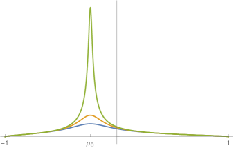
Figure 2: Circumference $\mathcal{C}$ of the metric on the spindle $\Sigma=\mathbb{WCP}^{1}_{[3,1]}$ on the conformal boundary as a function of $p\in[-1,1]$, for the supersymmetric non-extremal black holes. The blue, orange, and green curves have progressively smaller values of $\mathsf{Q}$, namely $\mathsf{Q}=0.04$, $\mathsf{Q}=0.01$ and $\mathsf{Q}=0.0002$, respectively, tending to the extremal solution with $\mathsf{Q}=0$. The same values of $\mathsf{Q}$ are plotted also in Figures 4 and 5.

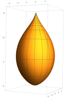
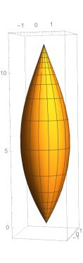
Figure 3: Embedding of two spindles on the conformal boundary for the supersymmetric non-extremal black holes in three dimensional Euclidean space. The left plot is for $\Sigma=\mathbb{WCP}^{1}_{[3,1]}$ and $\mathsf{Q}=0.04$ and the right plot is for $\Sigma=\mathbb{WCP}^{1}_{[3,2]}$ and $\mathsf{Q}=0.025$.

Introducing the orthonormal frame for the conformal boundary metric (6.37)

$$e^{0}=d\tau\,,\qquad e^{1}=-\frac{dp}{\sqrt{\mathcal{P}(p)}(1-\mathcal{P}(p))}\,,\qquad e^{2}=\sqrt{\frac{\mathcal{P}(p)}{1-\mathcal{P}(p)}}d\sigma\,,$$ (6.40)

we may solve the conformal Killing spinor equation (6.19) using the same basis of gamma matrices as the previous subsection (see below (6.19)). We find that

$$\zeta=\mathrm{e}^{-\mathrm{i}(\kappa_{1}\tau+\kappa_{2}\sigma)}\begin{pmatrix}\zeta_{1}(p)\\ \zeta_{2}(p)\end{pmatrix}\,,$$ (6.41)

where we have introduced the constants

$$\kappa_{1}=\frac{\mathsf{P}\mathsf{Q}}{2(\mathsf{P}^{2}+\mathsf{Q}^{2})}\,,\qquad\kappa_{2}=\frac{\mathsf{P}^{2}}{2(\mathsf{P}^{2}+\mathsf{Q}^{2})}\,.$$ (6.42)

Notice that in the extremal limit $\mathsf{Q}=0$ the phase in (6.41) is $\mathrm{e}^{-\mathrm{i}\sigma/2}=\mathrm{e}^{-\mathrm{i}\phi/2\alpha^{2}}$, which was compensated for in the previous subsection by making the gauge transformation (6.22). The components $\zeta_{1}(p)$, $\zeta_{2}(p)$ satisfy the equations

$$\begin{split}\zeta_{1}^{\prime}&=\frac{\mathrm{i}(p\mathsf{Q}-\kappa_{1})}{\sqrt{\mathcal{P}(p)}(1-\mathcal{P}(p))}\zeta_{1}\,,\\ \zeta_{2}&=\frac{4\mathrm{i}(p\mathsf{Q}-\kappa_{1})\mathcal{P}(p)-\sqrt{\mathcal{P}(p)}\mathcal{P}^{\prime}(p)}{4(p\mathsf{P}-\kappa_{2})\sqrt{\mathcal{P}(p)(1-\mathcal{P}(p))}}\zeta_{1}\,.\end{split}$$ (6.43)

After some effort, one finds the solution

$$\begin{split}\zeta_{1}(p)&=\sqrt{\frac{\mathcal{P}_{1}(p)-\mathcal{P}_{2}(p)-2\mathrm{i}\mathsf{Q}\sqrt{\mathcal{P}(p)}}{2\mathsf{P}\sqrt{1-\mathcal{P}(p)}}}\,,\\ \zeta_{2}(p)&=\sqrt{\frac{\mathcal{P}_{1}(p)-\mathcal{P}_{2}(p)+2\mathrm{i}\mathsf{Q}\sqrt{\mathcal{P}(p)}}{2\mathsf{P}\sqrt{1-\mathcal{P}(p)}}}\,.\end{split}$$ (6.44)

Notice that $\zeta_{1}^{*}=\zeta_{2}$ and $|\zeta_{1}|=|\zeta_{2}|$. In fact we have chosen the overall normalization constant of the spinor so that the components lie on the unit circle in the complex plane, namely $|\zeta_{1}|=|\zeta_{2}|=1$.

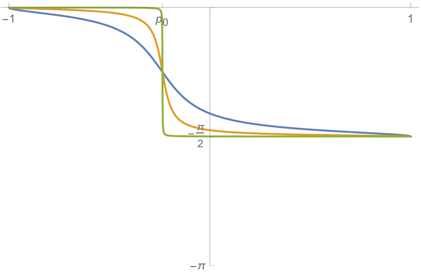
(a) $\mathrm{arg}\,\zeta_{1}(p)$

(b) $\mathrm{arg}\,\zeta_{2}(p)$

Figure 4: Arguments of $\zeta_{1}(p)$, $\zeta_{2}(p)$, appearing in the conformal Killing spinors on the conformal boundary for the supersymmetric non-extremal black holes, as a function of $p\in[-1,1]$ and plotted for the spindle $\Sigma=\mathbb{WCP}^{1}_{[3,1]}$ The blue, orange, and green curves have progressively smaller values of $\mathsf{Q}$, as given in Figure 2, tending to the extremal solution with $\mathsf{Q}=0$. For $\mathsf{Q}\neq 0$ we have a smooth conformal Killing spinor on the spindle that approaches two different constant values on each half of the spindle in the extremal limit $\mathsf{Q}\to 0$.

In Figure 4 we have plotted the arguments $\mathrm{arg}\,\zeta_{1}(p)$, $\mathrm{arg}\,\zeta_{2}(p)$, for the spindle $\Sigma=\mathbb{WCP}^{1}_{[3,1]}$ with progressively smaller values of $\mathsf{Q}$, tending to the extremal solution with $\mathsf{Q}=0$. In the latter case notice that in the $\mathsf{Q}\rightarrow 0$ limit we have

$$\mbox{for $\mathsf{Q}=0$:}\qquad\begin{cases}\ \mathrm{arg}\,\zeta_{2}(p)=-\mathrm{arg}\,\zeta_{1}(p)=\frac{\pi}{2}\,,&p\in(p_{0},1]\,,\\ \ \mathrm{arg}\,\zeta_{2}(p)=\mathrm{arg}\,\zeta_{1}(p)=0\,,&p\in[-1,p_{0})\,.\end{cases}$$ (6.45)

This precisely corresponds to the extremal solution (6.24).

We can also display the way in which the two different topological twists for the extremal case arise in the limit that $\mathsf{Q}\rightarrow 0$. In Figure 5 we have plotted the spin connection and gauge field for the conformal boundary geometries corresponding to Figure 4. More precisely, the non-trivial spin connection component is $\omega^{12}$, and we define its holonomy around a circle in the spindle $\Sigma$ at constant $p$, parametrized by $\sigma$, via

$$\omega(p)=\frac{1}{2\pi}\int_{S^{1}}\omega^{12}\,.$$ (6.46)

The solid curves in Figure 5 are then $\tfrac{1}{2}\omega(p)$, while the dashed lines are $\pm$ the corresponding holonomy of the gauge field $A+\kappa_{2}d\sigma$, cf. equation (6.23).

Figure 5: Spin connection and gauge field holonomies around a circle in the spindle $\Sigma$ for the supersymmetric non-extremal black holes, as a function of $p\in[-1,1]$ and plotted for the spindle $\Sigma=\mathbb{WCP}^{1}_{[3,1]}$. The dashed lines are $\pm$ the holonomy of the gauge field, while the solid blue, orange, and green lines are the corresponding holonomy of the spin connection for progressively smaller values of $\mathsf{Q}$, as given in Figure 2, tending to the extremal solution with $\mathsf{Q}=0$. For $\mathsf{Q}\neq 0$ we do not have a topological twist, but in the extremal limit $\mathsf{Q}\to 0$ we get a different topological twist on each half of the spindle.

Although the conformal boundary of this non-extremal supersymmetric solution is perfectly regular, in the bulk the black hole horizon has disappeared and there is a naked curvature singularity. To see this, we return to the black hole metric given in (6.1) in PD-type coordinates and observe that the function $\mathcal{Q}(q)$ has no real roots for $\mathsf{Q}\neq 0$. There is then a naked curvature singularity at $q=\infty$, with Penrose diagram given by Figure 6.

Figure 6: Penrose diagram for the non-extremal supersymmetric black holes, with $e\neq 0$. The black hole horizon has disappeared leaving a naked singularity. There is now a smooth conformal boundary which consists of the product of the time direction with a spindle.

6.3 A one-parameter family of non-supersymmetric and non-extremal solutions

In the previous two subsections we have discussed special cases that lie inside the more general class of non-rotating PD black holes. While interesting because they preserve supersymmetry, as discussed they both have some pathologies: either an acceleration horizon that cuts the conformal boundary, or a naked singularity. These pathologies arise because of the specific restrictions we have imposed on the parameters in those cases. According to the number and value of the roots of the functions $Q$ and $P$ there are many other possibilities. A detailed analysis of the causal structure in various cases can be found in [13]. In this subsection we will consider another special case that, while allowing some degree of analytic control over the roots of the metric functions, gives a black hole with completely regular conformal boundary, and two ordinary horizons. This configuration is also smoothly connected with the extremal and BPS black hole, thus providing a kind of “regulator” of the latter solution, while staying within the non-rotating family of solutions.

We start again with the general metric (3) with $a=0$, and we further restrict the parameters to satisfy

$$m=\frac{g}{\alpha}\,,\quad e=0\,,$$ (6.47)

and hence, in particular, we have $J=Q_{e}=0$. The first of the conditions in (6.47) is satisfied when both BPS conditions (6.1) are met, so it amounts to imposing only one of the two conditions. In addition, we recall that we imposed this condition in constructing regular uplifted solutions, as we discussed in section 4. The second is the extremality condition in the BPS case. It follows that the black hole that we obtain with these restrictions is neither BPS nor extremal, but it is continuously connected with the case discussed in section 6.1 by taking the limit

$$g\rightarrow g_{BPS}=\frac{\sqrt{1-\alpha^{2}}}{\alpha^{2}}\,.$$ (6.48)

Since we are taking $a=e=0$ in (3.3), we note that the gauge field is simply

$$A=-g\,\cos\theta\,d\phi\,.$$ (6.49)

We continue to take $\sqrt{3}/2<\alpha<1$ as in section 6.1, or equivalently $0<\mathsf{P}<1/2$ as in section 6.2. For fixed $\alpha$, the roots of $Q(r)$ depend on $g$ in a very simple way, as illustrated in Figure 7. In particular, we find:

• When $g>g_{BPS}$, $Q(r)$ has two real roots for negative $r$ which correspond to acceleration horizons, and no black hole horizon. As in section 6.1, the former intersect the conformal boundary, which causes pathologies: this can be seen from the fact that in this case the combination $1-\alpha^{2}\sin^{2}\theta\,P(\theta)$ appearing in the boundary metric (6.16) has two real roots, and is negative between the two.

• When $g<g_{BPS}$, $Q(r)$ has two real roots for positive $r$, which give two black hole horizons (an inner and an outer horizon) with no acceleration horizons. For this case $1-\alpha^{2}\sin^{2}\theta\,P(\theta)$ has no roots for $0\leq\theta\leq\pi$, which means the conformal boundary is a smooth spindle as in section 6.2.

• Finally, when $g=g_{BPS}$ then $Q(r)$ has two pairs of coincident real roots, which is the case discussed in section 6.1.

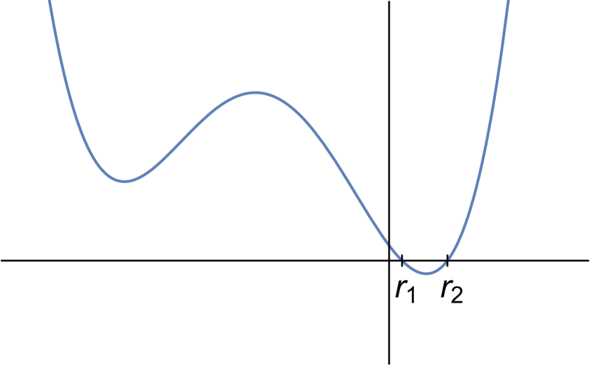
(a) $g<g_{BPS}$

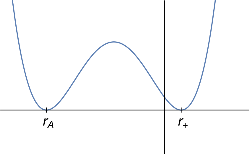
(b) $g=g_{BPS}$

(c) $g>g_{BPS}$

Figure 7: The function $Q(r)$ for three different cases in the class of non-supersymmetric and non-extremal black holes with $m=g/\alpha$ and $a=e=0$. We focus on the cases $g<g_{BPS}$ and $g=g_{BPS}$. When $g<g_{BPS}$ the two positive roots, $r_{1},r_{2}$, correspond to an inner and outer black hole horizon. When $g=g_{BPS}$ these two horizons coalesce to give an extremal horizon, $r_{+}$, and, in addition, an acceleration horizon, $r_{A}$, also appears. For $g>g_{BPS}$ there are no positive roots of $Q$, and hence no black hole horizon, but instead two negative roots which correspond to two acceleration horizons.

Since the main point of this section is showing that we can have an ordinary black hole with no acceleration horizons, we shall focus on the case

$$g<g_{BPS}\,.$$ (6.50)

Furthermore, note that while so far we have focused on the roots of $Q(r)$, the restrictions we have put on $\alpha$ and $g$ are also such as to guarantee $P(\theta)>0$ for $0\leq\theta\leq\pi$. Hence this case indeed corresponds to a completely regular black hole, whose Penrose diagram is given in Figure 8, where we have denoted by $r_{1,2}$ the two positive roots of $Q(r)$, with $r_{1}<r_{2}$. In the supersymmetric and extremal limit $g=g_{BPS}$ we have $r_{1}=r_{2}=r_{+}$.

Figure 8: Penrose diagram for the non-supersymmetric and non-extremal black holes with $m=g/\alpha$ and $a=e=0$ and $g<g_{BPS}$. In addition to the black hole event horizon, denoted by $r_{2}$, there is also an inner horizon, denoted by $r_{1}$. There is a smooth conformal boundary which consists of the product of the time direction with a spindle.

We can then require that the topology in the $\theta,\phi$ directions is that of a spindle $\Sigma=\mathbb{WCP}^{1}_{[n_{-},n_{+}]}$, by appropriately quantizing the conical deficits at $\theta=0,\pi$. This gives

$$\alpha=\sqrt{\frac{4\,n_{-}}{g(n_{-}-n_{+})}-\frac{2g+1}{g^{2}}}\,,$$ (6.51)

while the periodicity of $\phi$ is given by

$$\Delta\phi=\frac{\pi}{2\,g}\frac{n_{-}-n_{+}}{n_{-}\,n_{+}}\,.$$ (6.52)

As discussed above, in this case the black hole is completely smooth, and the spindle topology at fixed $t$ and $r$ persists to the conformal boundary, where the metric is again given by (6.16) and has the topology $\mathbb{R}\times\mathbb{WCP}^{1}_{[n_{-},n_{+}]}$. This is regular for any $0<g<g_{BPS}$, but degenerates as described in section 6.1 when $g$ approaches the BPS value. The behaviour of the circumference of the spindle at the boundary and of the spin connection of the boundary metric are very similar to those given in Figures 2 and 5, respectively. Namely, when $g\to g_{BPS}$, the spindle splits in half at

$$\theta=\theta_{0}\equiv\arccos\left(\frac{1-\sqrt{5-4\alpha^{2}}}{2\sqrt{1-\alpha^{2}}}\right)\,,$$ (6.53)

while the spin connection approaches $\pm$ the gauge field, up to the pure gauge term discussed in section 6.1.

7 Discussion

In this paper we have studied a very general class of four-dimensional dyonically charged, rotating, and accelerating black holes in four-dimensional anti-de Sitter space. The acceleration leads to conical deficit singularities at the horizon which can be taken to stretch out to the conformal boundary. When these conical deficits are appropriately “quantized”, so that the deficit angles are $2\pi(1-1/n_{\mp})$ with positive coprime integers $n_{\pm}$, the resulting space is known in the mathematics literature as a spindle, or equivalently a weighted projective space $\Sigma=\mathbb{WCP}^{1}_{[n_{-},n_{+}]}$. Remarkably, when uplifted to $D=11$ on a regular Sasaki-Einstein seven-manifold $SE_{7}$, the solutions become completely regular, free from any conical deficit singularities whatsoever. We have also quantized the flux of these $D=11$ solutions, thus showing that they give good M-theory backgrounds.

We have shown that there is a sub-family of both supersymmetric and extremal black hole solutions, which interpolate between $AdS_{4}$ in the UV and $AdS_{2}\times\Sigma$ in the near horizon IR limit. These are characterized by the integers $n_{\pm}$, that determine the spindle horizon geometry $\Sigma=\mathbb{WCP}^{1}_{[n_{-},n_{+}]}$, and a continuous parameter, which parametrizes both the electric charge $Q_{e}$ and the angular momentum $J$. The entropy of these black holes, which also carry magnetic charge (given in (4.31)), can be expressed simply in terms of $n_{\pm}$ and $Q_{e}$. We have shown that the entropy can be expressed in a number of equivalent ways, generalising previous expressions applicable for non-accelerating supersymmetric $AdS_{4}$ black holes. In particular, (5.25) reduces to the entropy of the extremal Kerr-Newman-AdS black hole upon setting $Q_{m}=0$ and $\chi=2$ (equivalently setting $n_{-}=n_{+}=1$ in (1.1)). The formula (5.22), which applies also to the Kerr-Newman-AdS black hole, highlights the dependence of the entropy on the angular momentum computed at the horizon. When uplifted, the near horizon limit gives a new class of rotating $AdS_{2}\times Y_{9}$ solutions, where we have shown that $Y_{9}$ may be viewed as either a regular $SE_{7}$ fibration over $\Sigma=\mathbb{WCP}^{1}_{[n_{-},n_{+}]}$, or equivalently as a Lens space $S^{3}/\mathbb{Z}_{\mathtt{q}}$ fibred over the $KE_{6}$ base of the $SE_{7}$. Remarkably, setting $Q_{e}=0$, which also sets $J=0$, these reduce to a known class of supersymmetric $AdS_{2}\times Y_{9}$ solutions first constructed in [1]. We have thus provided a new physical interpretation of those solutions: they are the near horizon limits of the accelerating (but non-rotating) black holes described in section 6, and we have generalized those solutions by adding angular momentum, preserving supersymmetry and extremality. It would be interesting to understand in more generality what kind of singularities in lower-dimensional supergravity theories can be uplifted to obtain regular solutions in higher dimensions. For example, it would be interesting to explore this for the $D=4$ black holes of [51, 52] which have non-compact horizons, but with finite entropy.

In this paper we have restricted our attention to solutions of minimal $D=4$ gauged supergravity. However, it is very likely that our constructions can be generalized to more general gauged supergravity theories with various matter content. More specifically, we expect to be able to construct supersymmetric spinning spindles which would generalize the constructions of [53], for example, where it was assumed that the horizon has spherical topology. We note the similarity of our formula for the black hole entropy (5.25) with eq. (54) of [53].

We now return to the holographic interpretation of the supersymmetric extremal black holes. The $D=11$ black hole solutions interpolate between $AdS_{4}\times SE_{7}$ in the UV and $AdS_{2}\times Y_{9}$ in the IR, where $Y_{9}$ is a $SE_{7}$ fibration over the spindle $\Sigma=\mathbb{WCP}^{1}_{[n_{-},n_{+}]}$. The $AdS_{4}\times SE_{7}$ vacuum solution describes $N_{SE}$ M2-branes at the Calabi-Yau four-fold singularity with conical metric $dr^{2}+r^{2}ds^{2}(SE_{7})$, and these typically have dual field theory descriptions as Chern-Simons quiver gauge theories, with the integer $N_{SE}$ determining the ranks of the gauge groups. Physically we are then wrapping the world-volume of the M2-branes over $\Sigma$. We have studied this conformal boundary geometry in some detail in section 6 for the non-rotating solutions with $Q_{e}=J=0$. An important subtlety in this case is that in the UV the conformal boundary is such that the spindle is split into two components. Moreover, in this limit supersymmetry is preserved via a different topological twist on each component. However, we have also shown that this split can be regulated in a family of non-rotating supersymmetric but non-extremal black holes (or by further relaxing the supersymmetry condition). Moreover, we do not expect the generic supersymmetric extremal rotating black holes, with $Q_{e}\neq 0$, to have this pathology. Indeed, in section 5 we have shown that the formula for the entropy of these black holes (5.7), is identical to that for the supersymmetric extremal Kerr-Newman family, obtained formally by setting $n_{-}=n_{+}=1$. On the other hand, the $Q_{e}=0$ solutions studied in section 6 are a somewhat degenerate limit.

With the above holographic interpretation, it should be possible to reproduce the black hole entropy formulae (1.1) by studying the dual M2-brane field theories. Indeed, there has been considerable progress on this topic for various classes of supersymmetric $AdS_{4}$ black holes. In particular, the first class of black holes for which a dual field theory interpretation has been found have just magnetic flux through a Riemann surface horizon $\Sigma$. The field theory calculation utilizes $I$-extremization, where the index can be identified with the localized partition function of the dual field theory on $S^{1}\times\Sigma$ [23, 24, 25, 26, 27, 28, 29, 30]. More recently, following the approach put forward in [54], progress has also been made in understanding the class of electrically charged and rotating $AdS_{4}$ black holes from the dual field theory point of view [39, 40, 41, 42]. For the accelerating black hole solutions that we discussed in this paper, it should be straightforward to now compute the suitably regularized on-shell action of the corresponding Euclidean solutions and reproduce the entropy by extremizing the corresponding entropy function. From the field theory side we should then focus on the Euclidean version of the conformal boundary geometry of the charged, rotating and accelerating black holes, and compute a certain twisted topological index associated with the $d=3$, $\mathcal{N}=2$ SCFTs on the M2-branes, wrapped on the spinning spindle $\Sigma$. While some care may be required in taking the BPS and extremal limit, it seems possible that we can get agreement between these computations using localization techniques in the large $N$ limit.

The wrapped M2-brane theories flow to a $d=1$ superconformal quantum mechanics in the IR, that is dual to the $AdS_{2}\times Y_{9}$ solutions that arise as the near horizon limit of the black holes. Equation (5.61) says that the $d=3$ superconformal R-symmetry mixes with the $U(1)$ isometry of the internal space $\Sigma$ in flowing to the $d=1$ superconformal R-symmetry in the IR. It should similarly be possible to reproduce this formula via a dual field theory/SCQM calculation by computing and then extremizing a suitable index. Indeed, in a companion paper [55] we study an analogous class of supersymmetric $D=5$ $AdS_{3}\times\Sigma$ solutions, with $\Sigma=\mathbb{WCP}^{1}_{[n_{-},n_{+}]}$ again a spindle, that uplift on a regular Sasaki-Einstein five-manifold to smooth solutions of type IIB supergravity. These are the holographic duals to D3-branes wrapping the spindle, and in this case we are able to reproduce both the central charge and the mixing of $d=4$ and $d=2$ superconformal R-symmetries in the supergravity solution, where in the field theory dual we make use of anomaly polynomials and $c$-extremization [56].

Acknowledgments

This work was supported in part by STFC grants ST/P000762/1, ST/T000791/1 and ST/T000864/1. JPG is supported as a Korea Institute for Advanced Study (KIAS) Scholar and as a Visiting Fellow at the Perimeter Institute for Theoretical Physics.

Appendix A Circle fibrations over spindles

In section 4.1 we showed that the $D=4$ PD black hole metrics uplift to regular $D=11$ solutions that on a fixed $t$, $r$ slice are topologically Lens space $S^{3}/\mathbb{Z}_{\mathtt{q}}$ bundles over the $KE_{6}$. On the other hand, we explained that this same space may also be viewed as an $SE_{7}$ fibration over a spindle/weighted projective space $\mathbb{WCP}^{1}_{[n_{-},n_{+}]}$. Fixing a point on the $KE_{6}$ implies that the Lens space fibre $S^{3}/\mathbb{Z}_{\mathtt{q}}$ is a circle bundle over the weighted projective space, where recall $\mathtt{q}=(k/I)(n_{-}-n_{+})$. In this appendix we spell this out in a little more detail, discussing circle bundles over spindles more generally.

We begin with $S^{3}$, embedded inside $\mathbb{C}^{2}$ as the unit sphere $S^{3}=\{|z_{1}|^{2}+|z_{2}|^{2}=1\}\subset\mathbb{C}^{2}$, with $z_{1},z_{2}$ standard complex coordinates. We may then consider the weighted circle action

$$(z_{1},z_{2})\rightarrow(\lambda^{n_{+}}z_{1},\lambda^{n_{-}}z_{2})\,,$$ (A.1)

where $\lambda=\mathrm{e}^{\mathrm{i}\theta}\in U(1)$, $n_{\pm}\in\mathbb{N}$, and note that for the action to be effective we need $\mathrm{hcf}(n_{+},n_{-})=1$. The quotient $S^{3}/U(1)=\mathbb{WCP}^{1}_{[n_{-},n_{+}]}$ is by definition a weighted projective space. This is a complex orbifold which is topologically a two-sphere with conical angles $2\pi/n_{\pm}$ at the poles. This is also known as a spindle. In terms of the action (A.1), the poles arise from $z_{2}=0$ and $z_{1}=0$, respectively, where in the first case all powers of the primitive $n_{+}-$th root of unity $\lambda=\mathrm{e}^{2\pi\mathrm{i}/n_{+}}$ act trivially, while in the second case this is true for $\lambda=\mathrm{e}^{2\pi\mathrm{i}/n_{-}}$.

It is a straightforward exercise to compute the Chern number of this fibration. That is, introduce a $(2\pi)$-period coordinate $\nu$ along the weighted $U(1)$ action, and corresponding connection one-form $\mathscr{A}$. This can be done starting from the round metric on $S^{3}$, with corresponding term $(\mathrm{d}\nu+\mathscr{A})^{2}$ for the metric on the circle fibre. The result is

$$\int_{\mathbb{WCP}^{1}_{[n_{-},n_{+}]}}\frac{\mathrm{d}\mathscr{A}}{2\pi}=\frac{1}{n_{+}n_{-}}\,,$$ (A.2)

where notice the overall sign is a matter of convention. By construction, the total space of this circle fibration over $\mathbb{WCP}^{1}_{[n_{-},n_{+}]}$ is $S^{3}$.

We may now consider a more general fibration with

$$\int_{\mathbb{WCP}^{1}_{[n_{-},n_{+}]}}\frac{\mathrm{d}\mathscr{A}}{2\pi}=\frac{\mathtt{r}}{n_{+}n_{-}}\,,$$ (A.3)

and $\mathtt{r}\in\mathbb{Z}$, and we will take $\mathtt{r}>0$ in what follows. We shall denote the corresponding complex line bundle, on which $\mathscr{A}$ is a connection, by $O(\mathtt{r})$. In terms of the original construction of $\mathbb{WCP}^{1}_{[n_{-},n_{+}]}$ as a quotient, notice that $\nu$ has period $2\pi/\mathtt{r}$. The total space of this circle fibration is then $S^{3}/\mathbb{Z}_{\mathtt{r}}$, where the $\mathbb{Z}_{\mathtt{r}}$ action is generated by

$$(z_{1},z_{2})\rightarrow(\omega_{\mathtt{r}}^{n_{+}}z_{1},\omega_{\mathtt{r}}^{n_{-}}z_{2})\,,$$ (A.4)

where $\omega_{\mathtt{r}}\equiv\mathrm{e}^{2\pi\mathrm{i}/\mathtt{r}}$ is a primitive $\mathtt{r}$th root of unity. In general the action (A.4) is not free. Specifically, the circle $S^{1}=\{z_{2}=0\}$ is fixed by $\mathbb{Z}_{\mathrm{hcf}(\mathtt{r},n_{+})}$, while the circle $S^{1}=\{z_{1}=0\}$ is fixed by $\mathbb{Z}_{\mathrm{hcf}(\mathtt{r},n_{-})}$. Thus the total space is a smooth manifold (rather than an orbifold) if and only if $\mathtt{r}$ has no common factor with either $n_{+}$ or $n_{-}$.

The main case of interest in the main text is when

$$\mathtt{r}=\mathtt{q}=\frac{k}{I}(n_{-}-n_{+})\,.$$ (A.5)

Recall here that $I/k$ is an integer that divides $n_{-}-n_{+}$. The gauged supergravity connection $2A$ is a connection on $O(\mathtt{q})$, as one sees for example in equation (5.16). Since $\mathrm{hcf}(n_{+},n_{-})=1$, it immediately follows that $\mathrm{hcf}(\mathtt{q},n_{\pm})=1$, and the total space of the circle fibration is smooth. In fact the construction in section 4.1 indirectly implies that this is diffeomorphic to the Lens space $S^{3}/\mathbb{Z}_{\mathtt{q}}=L(\mathtt{q},1)$. We may see this directly as follows. Since $\mathrm{hcf}(\mathtt{q},n_{+})=1$, we can find integers $a,b\in\mathbb{Z}$ such that $an_{+}+b\mathtt{q}=1$. It follows that $a\frac{n_{+}}{\mathtt{q}}=-b+\frac{1}{\mathtt{q}}$, and hence

$$(\omega_{\mathtt{q}}^{n_{+}})^{a}=\mathrm{e}^{2\pi\mathrm{i}an_{+}/\mathtt{q}}=\omega_{\mathtt{q}}\,.$$ (A.6)

Thus the $\mathbb{Z}_{\mathtt{q}}$ action (A.4) is equivalent to

$$(z_{1},z_{2})\rightarrow(\omega_{\mathtt{q}}z_{1},\omega_{\mathtt{q}}^{an_{-}}z_{2})\,,$$ (A.7)

which is the definition of the Lens space $L(\mathtt{q},an_{-})$. On the other hand, we have $an_{-}=a\left(n_{+}+\frac{I}{k}\mathtt{q}\right)=1+\mathtt{q}(\frac{I}{k}a-b)\cong 1$ mod $\mathtt{q}$. Thus $L(\mathtt{q},an_{-})\cong L(\mathtt{q},1)=S^{3}/\mathbb{Z}_{\mathtt{q}}$, as we wanted to show.

Appendix B Non-accelerating case: $\alpha=0$

The principal focus of this paper is to study accelerating black holes with $\alpha\neq 0$. However, for completeness we discuss here the case when $\alpha=0$, also known as the Kerr-Newman-AdS spacetime [36].

We set $\alpha=0$ in (3) and then rescale

$$\phi=\varphi\,\Xi^{-1}\,,$$ (B.1)

with $\Xi=1-a^{2}$, to ensure that the metric is well-defined at $\theta=0$ and $\theta=\pi$, with $\varphi\in[0,2\pi)$. The metric now reads

$$ds^{2}=-\frac{Q}{\Sigma}\big{(}dt-\frac{a\sin^{2}\theta}{\Xi}\,d\varphi\big{)}^{2}+\frac{\Sigma}{Q}\,dr^{2}+\frac{\Sigma}{P}d\theta^{2}+\frac{P}{\Sigma}\sin^{2}\theta\big{(}adt-\frac{r^{2}+a^{2}}{\Xi}d\varphi\big{)}^{2},$$ (B.2)

with

$$\Sigma =r^{2}+a^{2}\cos^{2}\theta\,,$$

$$P =1-a^{2}\cos^{2}\theta\,,$$

$$Q =(r^{2}+a^{2})(1+r^{2})-2mr+e^{2}+g^{2}\,,$$ (B.3)

and the gauge field given by

$$A=-e\frac{r}{\Sigma}\big{(}dt-\frac{a\sin^{2}\theta}{\Xi}d\varphi\big{)}+g\frac{\cos\theta}{\Sigma}\big{(}adt-\frac{r^{2}+a^{2}}{\Xi}d\varphi\big{)}\,.$$ (B.4)

When $\alpha=0$, the conditions for preservation of supersymmetry need to be carried out again. We find that the integrability conditions now give the BPS constraints

$$0= \,m\,g\,,$$ (B.5)

$$0= \,e^{4}-2a^{2}e^{4}+a^{4}e^{4}+2e^{2}g^{2}-4a^{2}e^{2}g^{2}+2a^{4}e^{2}g^{2}-4e^{4}g^{2}+g^{4}-2a^{2}g^{4}+a^{4}g^{4}$$

$$-8e^{2}g^{4}-4g^{6}-2e^{2}m^{2}-2a^{2}e^{2}m^{2}-2g^{2}m^{2}-2a^{2}g^{2}m^{2}+m^{4}\,.$$ (B.6)

With $m>0$ we therefore take $g=0$. The second equation can then be solved and with $a,e\geq 0$ we conclude that for BPS black holes we should take

$$g=0\,,\qquad m=(1+a)e\,.$$ (B.7)

By studying the roots of $Q$ we can determine that we have an extremal BPS black hole provided that

$$e=\sqrt{a}(1+a)\,,$$ (B.8)

and hence

$$m=\sqrt{a}(1+a)^{2}\,,$$ (B.9)

with the horizon at $r_{+}=\sqrt{a}$. From (3.14) we can then write the total electric charge as

$$G_{(4)}Q_{e}=\frac{\sqrt{a}}{1-a}\,,$$ (B.10)

and from (E.6) the total angular momentum is

$$G_{(4)}J =\frac{a\sqrt{a}}{(1-a)^{2}}=\frac{G_{(4)}Q_{e}}{2}\left(\sqrt{1+4(G_{(4)}Q_{e})^{2}}-1\right)\,.$$ (B.11)

Note that when $\alpha=0$, this expression for the angular momentum, in the gauge we are using, can also be obtained from a Komar integral (E.1), as is often used in the literature. Finally, from (3.12) the entropy of these black holes is given by

$$S_{BH} =\frac{\pi}{G_{(4)}}\frac{a}{1-a}=\frac{\pi}{2G_{(4)}}(\sqrt{1+4(G_{(4)}Q_{e})^{2}}-1)=\frac{\pi}{G_{(4)}}\frac{J}{Q_{e}}\,,$$ (B.12)

in agreement with the literature.

Appendix C Near horizon limit

In this appendix we shall consider the near horizon limit of the PD solution (3)–(3.3), in the BPS and extremal case. To this end, we first write the function $Q(r)$ as

$$Q(r)=(r-r_{+})^{2}\,\left(x_{0}+x_{1}\,r+x_{2}\,r^{2}\right),$$ (C.1)

where the constants $x_{i}$ are defined by

$$x_{0} =-\alpha^{2}\left(a^{2}+e^{2}+g^{2}\right)+a^{2}+4\alpha\,g\,r_{+}-3\left(\alpha^{2}-1\right)r_{+}^{2}+1\,,$$

$$x_{1} =2\alpha\,g-2\left(\alpha^{2}-1\right)r_{+}\,,$$

$$x_{2} =1-\alpha^{2}\,.$$ (C.2)

The horizon radius, $r_{+}$, is subject to the following condition:

$$-4\alpha\left(a^{2}+e^{2}\right)+4\alpha^{3}\left(a^{2}+e^{2}+g^{2}\right)-5\alpha g^{2}$$

$$+g\left(\left(a^{2}-5\right)\alpha^{2}+\alpha^{4}\left(-\left(a^{2}+e^{2}+g^{2}\right)\right)+6\right)\,r_{+}$$

$$+\alpha\left(-2a^{2}\left(\alpha^{2}-1\right)^{2}-2\alpha^{4}\left(e^{2}+g^{2}\right)+\alpha^{2}\left(2e^{2}+5g^{2}+2\right)-2\right)\,r_{+}^{2}=0\,,$$ (C.3)

with the parameters obeying the BPS constraints.

A convenient way to find the near horizon solution is to implement the following coordinate transformation,

$$r\to r_{+}+\lambda\,s\,\rho\,,\quad t\to\lambda^{-1}\,s\,\tau\,,\quad\phi\to\phi^{\prime}+\lambda^{-1}\,s\,W\frac{\Delta\phi}{2\pi}\,\tau\,,$$ (C.4)

where $s$ is a constant, and then take the $\lambda\to 0$ limit. Here $W$ is given by

$$W=\frac{a}{r_{+}^{2}+a^{2}}\frac{2\pi}{\Delta\phi}\,,$$ (C.5)

with $\partial_{t}+W\frac{\Delta\phi}{2\pi}\partial_{\phi}=\partial_{t}+W\partial_{\varphi}$ a null generator of the horizon. It is convenient to choose

$$s=\sqrt{\frac{r_{+}^{2}+a^{2}}{x_{0}+x_{1}\,r_{+}+x_{2}\,r_{+}^{2}}}\,,$$ (C.6)

and we then find that the near horizon metric reads, after dropping the primes from the new coordinates,

$$ds^{2}_{4}={\lambda}(\theta)\,\left(-r^{2}\,dt^{2}+\frac{dr^{2}}{r^{2}}\right)+\frac{d\theta^{2}}{\tilde{P}(\theta)}+\frac{(r_{+}^{2}+a^{2})^{2}\,\sin^{2}\theta\,\tilde{P}(\theta)}{(1-\alpha\,r_{+}\,\cos\theta)^{4}}\,\left(d\phi+vr\,dt\right)^{2},$$ (C.7)

where

$$\tilde{\lambda}(\theta) =\frac{a^{2}\cos^{2}\theta+r_{+}^{2}}{\left(1-\alpha r_{+}\cos\theta\right){}^{2}\left(x_{0}+x_{1}\,r_{+}+x_{2}\,r_{+}^{2}\right)}\,,$$

$$\tilde{P}(\theta) =\frac{\left(1-\alpha r_{+}\cos\theta\right){}^{2}}{a^{2}\cos^{2}\theta+r_{+}^{2}}\,P(\theta)\,,$$

$$v =\frac{2ar_{+}}{\left(a^{2}+r_{+}^{2}\right)\left(x_{0}+x_{1}\,r_{+}+x_{2}\,r_{+}^{2}\right)}\,.$$ (C.8)

For the gauge field, we find that there is a piece that is singular in the $\lambda\to 0$ limit, but it can be removed by a gauge transformation. We thus implement the gauge transformation

$$A\to A-\frac{s\,r_{+}\,e}{\lambda\left(a^{2}+r_{+}^{2}\right)}\,dt-\frac{e(a^{2}-r_{+}^{2})}{2ar_{+}}d\phi\,,$$ (C.9)

where the second term is included for convenience. Taking the $\lambda\to 0$ limit we then obtain the near horizon gauge field

$$A=-\frac{\left(a^{2}+r_{+}^{2}\right)\left(a^{2}e\cos^{2}\theta+2agr_{+}\cos\theta-er_{+}^{2}\right)}{2ar_{+}\left(a^{2}\cos^{2}\theta+r_{+}^{2}\right)}\,\left(d\phi+v\,r\,dt\right)\,.$$ (C.10)

We can now show that the near horizon metric (C.7) and gauge field (C.10) are equivalent to the solution (5.1). The easiest way to see this is to start from (C.7), and perform the following coordinate transformations:

$$\tau\to-t\,,\quad\rho\to r\,,\quad y\to\frac{c_{1}+c_{2}\,\cos\theta}{1-\alpha\,r_{+}\,\cos\theta}\,,\quad z\to-\kappa\,\phi\,,$$ (C.11)

where

$$c_{1} =\frac{2\,\alpha\,r_{+}^{3}}{\sqrt{\left(x_{0}+x_{1}\,r_{+}+x_{2}\,r_{+}^{2}\right)\left(a^{2}+\alpha^{2}\,r_{+}^{4}\right)}}\,,$$

$$c_{2} =\frac{2\,a^{2}}{\sqrt{\left(x_{0}+x_{1}\,r_{+}+x_{2}\,r_{+}^{2}\right)\left(a^{2}+\alpha^{2}\,r_{+}^{4}\right)}}\,,$$

$$\kappa =\sqrt{\frac{x_{0}+x_{1}\,r_{+}+x_{2}\,r_{+}^{2}}{a^{2}+\alpha^{2}\,r_{+}^{4}}}\,\left(r_{+}^{2}+a^{2}\right)\,.$$ (C.12)

The parameters are then identified as follows:

$$\mathtt{j} =\frac{2\,a\,r_{+}}{\sqrt{\left(x_{0}+x_{1}\,r_{+}+x_{2}\,r_{+}^{2}\right)\left(a^{2}+\alpha^{2}\,r_{+}^{4}\right)}}\,,$$

$$\mathtt{a} =4\frac{-a^{2}\,g+2\,a\,e\,\alpha\,r_{+}^{2}+g\,\alpha^{2}\,r_{+}^{4}}{\left(x_{0}+x_{1}\,r_{+}+x_{2}\,r_{+}^{2}\right)\left(a^{2}+\alpha^{2}\,r_{+}^{4}\right)}\,.$$ (C.13)

Let us now turn to the non-rotating case, $a=0$. As discussed in section 6.1, in the BPS and extremal limit we can express all parameters and horizon radius in terms of $\alpha$ via

$$e=0\,,\quad g=\frac{\sqrt{1-\alpha^{2}}}{\alpha^{2}}\,,\quad m=\frac{\sqrt{1-\alpha^{2}}}{\alpha^{3}}\,,\quad r_{+}=\frac{\sqrt{5-4\alpha^{2}}-1}{2\alpha\sqrt{1-\alpha^{2}}}\,.$$ (C.14)

With $Q(r)=(r-r_{+})^{2}\,(x_{0}+x_{1}\,r_{+}+x_{2}\,r_{+}^{2})$, we can now obtain simple expressions for $x_{0},x_{1},x_{2}$:

$$x_{0} =\frac{-2\alpha^{2}+\sqrt{5-4\alpha^{2}}+3}{2\alpha^{2}}\,,\quad x_{1}=\frac{\sqrt{1-\alpha^{2}}\left(\sqrt{5-4\alpha^{2}}+1\right)}{\alpha}\,,$$

$$x_{2} =1-\alpha^{2}\,.$$ (C.15)

We then take the near horizon limit with the coordinate transformation (C.4), where we note that now since $a=0$ we have $W=0$, as expected since we have switched off rotation. Taking the limit $\lambda\to 0$, and again dropping the primes from the new coordinates, we get the near horizon metric

$$ds^{2} =\frac{r_{+}^{2}}{\left(1-\alpha\,r_{+}\,\cos\theta\right)^{2}}\bigg{[}\frac{1}{x_{0}+x_{1}\,r_{+}+x_{2}\,r_{+}^{2}}\,\left(-r^{2}\,dt^{2}+\frac{dr^{2}}{r^{2}}\right)$$

$$\qquad\qquad\qquad\qquad\qquad+\frac{d\theta^{2}}{P(\theta)}+P(\theta)\,\sin^{2}\theta\,d\phi^{2}\bigg{]}\,,$$ (C.16)

and gauge field

$$A=-g\,\cos\theta\,d\phi\,,$$ (C.17)

where we recall that all parameters are constrained by the BPS and extremality conditions (C.14). It can be shown that this solution is equivalent to the non-rotating case ($\mathtt{j}=0$) of the metric (5.1). To see this, starting from (5.1) with $\mathtt{j}=0$, one needs to change coordinates and identify the parameters as follows:

$$\tau \to-t\,,\quad\rho\to r\,,\quad y\to\frac{2\left(\sqrt{5-4\alpha^{2}}-1\right)}{\sqrt{5-4\alpha^{2}}\left(\left(1-\sqrt{5-4\alpha^{2}}\right)\cos\theta+2\sqrt{1-\alpha^{2}}\right)}\,,$$

$$z \to-\frac{\sqrt{5-4\alpha^{2}}}{\alpha^{2}}\,\phi\,,\quad\mathtt{a}\to\frac{4\sqrt{1-\alpha^{2}}}{5-4\alpha^{2}}\,.$$ (C.18)

Recall that $\sqrt{3}/2<\alpha<1$, which corresponds to the range $0<\mathtt{a}<1$.

Appendix D The $AdS_{2}\times Y_{9}$ solutions of [1]

We briefly outline how the $D=11$ $AdS_{2}\times Y^{9}$ solutions found in [1] and further discussed in appendix D of [48] can also be viewed as solutions of $D=4$ minimal gauged supergravity. The analysis of regularity and flux quantization which was carried out in [48] is different to what we have done in this paper, and we explain how they are related.

Consider the metric $ds^{2}(Y_{9})$ given in (3.36) of [1]:

$$ds^{2}(Y_{9})=w(y)Dz^{2}+\frac{q(y)}{y^{6}w(y)}D\psi^{2}+\frac{4}{q(y)}dy^{2}+\frac{16}{y^{2}}ds^{2}_{KE_{6}}\,,$$ (D.1)

where $Dz=dz-g(y)D\psi$, $D\psi=d\psi+4B$, with $dB=2J$ and

$$q(y) =y^{4}-4y^{2}+4{\mathtt{a}}y-{\mathtt{a}}^{2}\,,$$

$$g(y) =\frac{{\mathtt{a}}-y}{y^{3}-3y+2{\mathtt{a}}}\,,$$

$$w(y) =\frac{y^{3}-3y+2{\mathtt{a}}}{y^{3}}\,.$$ (D.2)

If we complete the square using the $\psi$ coordinate we immediately find

$$ds^{2}(Y_{9})=\frac{1}{y^{2}}\Big{[}D\psi+(1-\frac{\mathtt{a}}{y})dz\Big{]}^{2}+\frac{4}{q}dy^{2}+\frac{q}{y^{4}}dz^{2}+\frac{16}{y^{2}}ds^{2}_{KE_{6}}\,.$$ (D.3)

Assembling the $D=11$ metric, as described in [1], we obtain

$$ds^{2}_{11} =\frac{2}{3}\left[y^{2}ds^{2}(AdS_{2})+\frac{4y^{2}}{q}dy^{2}+\frac{q}{y^{2}}dz^{2}+\Big{[}D\psi+(1-\frac{\mathtt{a}}{y})dz\Big{]}^{2}+16ds^{2}_{KE_{6}}\right]\,,$$

$$=\frac{32}{3}\Bigg{[}\frac{1}{4}\Big{\{}\frac{y^{2}}{4}ds^{2}(AdS_{2})+\frac{y^{2}}{q}dy^{2}+\frac{q}{4y^{2}}dz^{2}\Big{\}}$$

$$\qquad\qquad\qquad+\Big{\{}\Big{[}\frac{1}{4}d\psi+B+\frac{1}{4}(1-\frac{\mathtt{a}}{y})dz\Big{]}^{2}+ds^{2}_{KE_{6}}\Big{\}}\Bigg{]}\,.$$ (D.4)

Comparing this with (2) we see this is precisely of the form to give a solution of minimal $D=4$ gauged supergravity with

$$ds^{2}_{4} =\frac{y^{2}}{4}ds^{2}(AdS_{2})+\frac{y^{2}}{q}dy^{2}+\frac{q}{4y^{2}}dz^{2},$$

$$A =\frac{1}{2}(1-\frac{\mathtt{a}}{y})dz\,,$$ (D.5)

after choosing $L=(32/3)^{1/2}$. Finally, as a check, the four-form flux in [1] can be written as

$$G=\left(\frac{32}{3}\right)^{3/2}\left[\tfrac{3}{8}\mathrm{vol}_{4}-\tfrac{1}{2}*_{4}F\wedge J\right]\,,$$ (D.6)

in agreement with (2).

We now return to the metric as written in (D.1) and recall the analysis demonstrating regularity, as discussed in [1]. The analysis of [1] begins by showing that after taking $\Delta\psi=2\pi$, then $\psi,y$ parametrize a smooth two-sphere. Then one shows that this two-sphere can be fibred over the $KE_{6}$ space to give an eight-dimensional manifold. Next, by choosing the period of $z$ to be $2\pi l$, for suitably defined $l$, we obtain a good circle fibration over the eight-dimensional manifold. To implement the latter one shows that the periods over a basis of two-cycles on the eight-dimensional space are suitably quantized. A basis can be taken to be the $S^{2}$ fibre at a fixed point on the $KE_{6}$ together with a basis of two-cycles on $KE_{6}$ sitting at the one of two poles on the $S^{2}$, say $y=y_{2}$. The conditions are satisfied if and only if

$$g(y_{3})-g(y_{2})=l\mathtt{q}\,,\qquad g(y_{2})=l\mathtt{p}/I\,,\qquad$$ (D.7)

with integers $\mathtt{p},\mathtt{q}$. If $\mathtt{p},\mathtt{q}$ have no common factor then the nine-dimensional space $Y_{9}$ is simply-connected. As shown in [1] these conditions imply

$$\mathtt{a} =\frac{I\mathtt{q}(2\mathtt{p}+I\mathtt{q})}{2\mathtt{p}^{2}+2I\mathtt{p}\mathtt{q}+I^{2}\mathtt{q}^{2}}\,,$$

$$l^{2} =\frac{I^{2}(2\mathtt{p}^{2}+2I\mathtt{p}\mathtt{q}+I^{2}\mathtt{q}^{2}}{2\mathtt{p}^{2}(\mathtt{p}+I\mathtt{q})^{2}}\,.$$ (D.8)

This construction can also be viewed as a fibration of a Lens space $S^{3}/\mathbb{Z}_{\mathtt{q}}$ over the $KE_{6}$. To see this more explicitly we can use canonical coordinates on $S^{3}/\mathbb{Z}_{\mathtt{q}}$, with the $\mathbb{Z}_{\mathtt{q}}$ identification acting on a Hopf fibre coordinate. We consider $\psi=\gamma$ and $z=\bar{\alpha}+\lambda\gamma$ and we fix the constant $\lambda$ momentarily. Observe that this implies $\partial_{\psi}=\partial_{\gamma}-\lambda\partial_{\bar{\alpha}}$ and $\partial_{z}=\partial_{\bar{\alpha}}$. In the new coordinates the metric reads

$$ds^{2}_{Y_{9}}=w(y)(d\bar{\alpha}-\tilde{g}D\gamma-4\lambda B)^{2}+\frac{q}{y^{6}w(y)}D\gamma^{2}+\frac{4}{q}dy^{2}+\frac{16}{y^{2}}ds^{2}_{KE_{6}}\,,$$ (D.9)

with $D\gamma=d\gamma+4B$ and $\tilde{g}(y)\equiv g(y)-\lambda$. If we take $\Delta\gamma=2\pi$ then $\gamma,y$ again parametrize an $S^{2}$, which is fibred over the $KE_{6}$ manifold. We now consider the $\bar{\alpha}$ circle fibred over this eight-dimensional base. To see the Lens space structure, we fix a point on the $KE_{6}$ base and fix the constant $\lambda$ by demanding $\tilde{g}(y_{3})+\tilde{g}(y_{2})=0$, which ensures that $\bar{\alpha}$ is a Hopf fibre coordinate on the resulting $S^{3}/\mathbb{Z}_{\mathtt{q}}$. More specifically, we choose $\lambda=\frac{l}{2}(\mathtt{q}+2\mathtt{p}/I)$ and then we have

$$\tilde{g}(y_{3})=-\tilde{g}(y_{2})=\frac{l\mathtt{q}}{2}\,.$$ (D.10)

Taking $\Delta\gamma=2\pi$ and $\Delta\bar{\alpha}=2\pi l$ then implies that we have an $S^{3}/\mathbb{Z}_{\mathtt{q}}$ fibre. That the $S^{3}/\mathbb{Z}_{\mathtt{q}}$ is suitably fibred over the $KE_{6}$ base is easily demonstrated: taking a basis of two-cycles, $\Sigma_{a}(y_{2}),$ to be again located at $y=y_{2}$, for example we calculate

$$\frac{1}{2\pi l}\int_{\Sigma_{a}(y_{2})}d[d\bar{\alpha}-\tilde{g}D\gamma-4\lambda B] =-\frac{1}{2\pi l}(\tilde{g}(y_{2})+\lambda)\int_{\Sigma_{a}(y_{2})}\rho$$

$$=-\mathtt{p}s_{a}\,,$$ (D.11)

for integers $s_{a}$.

We can also introduce coordinates on $S^{3}/\mathbb{Z}_{\mathtt{q}}$ via $\bar{\alpha}_{\pm}=\gamma\mp\frac{1}{l\mathtt{q}}\bar{\alpha}$. In these coordinates we can write the vectors in the original $\psi,z$ coordinates as $\partial_{z}=-\frac{1}{lq}(\partial_{+}-\partial_{-})$ and $\partial_{\psi}=\partial_{+}+\frac{\mathtt{p}}{I\mathtt{q}}(\partial_{+}-\partial_{-})$, with the latter directly analogous to (4.18). This underscores that while in the regularity construction using the $z,\psi$ coordinates, $\Delta\psi=2\pi$ was required to ensure that $y,\psi$ formed an $S^{2}$, it is not the case, in general, that $\psi$ is a periodic coordinate on the three-dimensional Lens space, i.e. under the motion of $\partial_{\psi}$ by $2\pi$ one does not return to the same point.

A final point is that the R-symmetry Killing vector can be obtained from [1], and we find that it is given by

$$R=2\partial_{\psi}+2\partial_{z}\,.$$ (D.12)

This agrees with our general formula (5.61) in the $\mathtt{j}=0$ limit.

Appendix E Angular momentum

In this section we discuss the angular momentum of the PD black holes (3), (3.3). We will also calculate the angular momentum of the near horizon $AdS_{2}$ solutions that we constructed in appendix C, and explain how these two quantities differ in general. Finally, we shall derive the formula (1.2).

A common way of defining the angular momentum is via a Komar integral associated to the spacelike Killing vector $k=\partial_{\varphi}$, where $\varphi$ is the angular coordinate on the spindle with period $2\pi$ (see (3.10)). For the associated one-form $k$ one takes

$$J_{K}(r) \equiv\frac{1}{16\pi G_{(4)}}\int_{\Sigma_{r}}\ast dk\,,$$ (E.1)

where the integral is over the surface $\Sigma_{r}$, parametrized by $\theta,\phi$ at fixed $r$ and $t$. While this integral is gauge invariant, it clearly depends on the radial coordinate $r$ since, in general, $d*dk\neq 0$.

Instead we will adopt a different definition which does not depend on the radial position where the integral is done, and hence it can equally be evaluated at the black hole horizon. While this an attractive feature, and is the definition that is expected to appear in the First Law [22], the price we pay is that the integral changes under gauge transformations. We first define the two-form

$$Z=dk+4(A\cdot k)F\,,$$ (E.2)

for an arbitrary Killing vector $k$ which satisfies, on-shell,

$$\nabla_{\mu}Z^{\mu\nu}=-k^{\nu}\mathcal{L}\,,$$ (E.3)

where $\mathcal{L}$ is the Lagrangian. For $k=\partial_{\varphi}$ we can then define the angular momentum via the horizon integral

$$J(A)=\frac{1}{16\pi G_{(4)}}\int_{\Sigma_{r_{+}}}*Z\,.$$ (E.4)

With the gauge field as in (3.3), we obtain

$$J\equiv J(A)=\frac{1}{G_{(4)}}{m\,a}\,\left(\frac{\Delta\phi}{2\pi}\right)^{2}\,.$$ (E.5)

For the simpler case of the Kerr-Newman-AdS black holes with $\alpha=0$ as in (B.2), we then have

$$G_{(4)}J=\frac{ma}{(1-a^{2})^{2}}\,,$$ (E.6)

in agreement with the results given in [22, 41], for example. Note also that for the case of $\alpha=0$, the expressions (E.5), (E.6) can also be obtained from the Komar integral (E.1); we have not checked whether this also happens to be true when $\alpha\neq 0$ (and one should be aware that the conformal boundary is not obtained simply by taking $r\to\infty$).

We would also like to calculate the angular momentum using the near horizon $AdS_{2}$ solution (5.1). However, (E.4) is not gauge invariant and since in the derivation of (5.1) we performed some gauge transformations (see in particular eq. (C.9)), some care is required. We first note that if we consider gauge transformations of the form

$$\tilde{A}=A+\alpha_{1}\,dt+\alpha_{2}\,d\phi\,,$$ (E.7)

for constant $\alpha_{i}$, then

$$J(\tilde{A})=J(A)+\alpha_{2}\,Q_{e}\frac{\Delta\phi}{2\pi}\,.$$ (E.8)

Notice, in particular, that this does not depend on $\alpha_{1}$. Demanding that the gauge field of the full black hole solution is regular on the horizon effectively fixes $\alpha_{1}$, as we explain in section E.1. However, the freedom in choosing $\alpha_{2}$ is associated with how one defines the electric potential, as we discuss in section E.2. In section E.3 we then calculate the angular momentum for the near horizon $AdS_{2}$ solution (5.1) and explain how it is related to that of the black hole (E.5). Finally, in section E.4 we briefly make some comments concerning the dual conformal field theory (CFT).

E.1 Regularity of the gauge field on the horizon

We now investigate the gauge transformation that is required in order to ensure that the full black hole solution (3), (3.3) is well-defined on the horizon of the black hole. To do so, we Wick rotate $t\to\mathrm{i}\,t_{E}$, as well as $a\to\mathrm{i}\,a_{E},\,\,e\to\mathrm{i}\,e_{E}$, and define the Euclidean angular velocity

$$\Omega_{E} \equiv\mathrm{i}\,W\equiv-\frac{a_{E}}{r_{+}^{2}-a_{E}^{2}}\frac{2\pi}{\Delta\phi}\,.$$ (E.9)

We next change coordinates $t_{E}\to\tilde{t}_{E}$ and $\phi\to\tilde{\phi}+\frac{\Delta\phi}{2\pi}\Omega_{E}\,t_{E}$, and consider the metric near the horizon $r\sim r_{+}$, where $r_{+}$ is the outer horizon, defined by the largest positive root of ${Q}(r)$. We find

$$ds^{2}\simeq(r-r_{+})f(\theta)d\tilde{t}_{E}^{2}+\frac{f(\theta)}{4\kappa^{2}\,(r-r_{+})}dr^{2}+h(\theta)d\tilde{\phi}^{2}+(r-r_{+})\,g(\theta)\,d\tilde{\phi}\,d\tilde{t}_{E}\,,$$ (E.10)

with $\kappa$ the surface gravity. Changing variables via

$$x=\sqrt{r-r_{+}}\,\cos(\kappa\,\tilde{t}_{E})\,,\qquad y=\sqrt{r-r_{+}}\,\sin(\kappa\,\tilde{t}_{E})\,,$$ (E.11)

with $(x,y)$ parametrising $\mathbb{R}^{2}$, we get

$$ds^{2}\simeq\frac{f(\theta)}{\kappa^{2}}(dx^{2}+dy^{2})+\frac{g(\theta)}{\kappa}(x\,dy-y\,dx)d\tilde{\phi}+h(\theta)d\tilde{\phi}^{2}\,,$$ (E.12)

which is clearly regular near the origin $x=y=0$.

For the gauge field given in (3.3), we find

$$A =f_{1}(r,\theta)d\tilde{t}_{E}+f_{2}(r,\theta)d\tilde{\phi}\,,$$

$$=\frac{f_{1}(r,\theta)}{\kappa}\frac{x\,dy-y\,dx}{x^{2}+y^{2}}+f_{2}(r,\theta)d\tilde{\phi}\,.$$ (E.13)

Since $f_{2}(r_{+},\theta)$ is finite, the last term is well behaved at the horizon. However, in the gauge (3.3) we find that $f_{1}(r,\theta)$ does not vanish fast enough as $r\to r_{+}$ to ensure regularity. Let us consider the gauge transformation given in (E.7) and choose

$$\alpha_{1}=\frac{r_{+}\,e}{r_{+}^{2}+a^{2}}-\frac{\Delta\phi}{2\pi}W\alpha_{2}\,,$$ (E.14)

with $\alpha_{2}$ arbitrary. We then find

$$\tilde{A}=\frac{\tilde{f}_{1}(r,\theta)}{\kappa}\frac{x\,dy-y\,dx}{x^{2}+y^{2}}+\left(f_{2}(r,\theta)+\alpha_{2}\right)\,d\tilde{\phi}\,,$$ (E.15)

with $\tilde{f}_{1}(r,\theta)\equiv f_{1}(r,\theta)-\frac{r_{+}\,e_{E}}{r_{+}^{2}-a_{E}^{2}}$ and, as $r\to r_{+}$,

$$\tilde{f}_{1}(r,\theta)\sim(r-r_{+})F(\theta)=(x^{2}+y^{2})\,F(\theta)\,.$$ (E.16)

Thus, this gauge field $\tilde{A}$ is regular on the horizon, for any value of $\alpha_{2}$. As we discussed above, the choice of $\alpha_{1}$ does not affect the value of the angular momentum of the black hole, $J(A)$ as defined in (E.4), but the choice of $\alpha_{2}$ will.

Notice that the value of $\alpha_{1}$ in (E.14) with $\alpha_{2}$ given by

$$\alpha_{2}=\frac{e(a^{2}-r_{+}^{2})}{2ar_{+}}\,,$$ (E.17)

exactly matches the gauge transformation that we performed in (C.9). That the value of $\alpha_{1}$ agrees is exactly as expected, since this is the gauge transformation which was required in that analysis in order to have a regular gauge field in the near horizon limit. The last term in (C.9) corresponds to the specific choice of $\alpha_{2}$ given in (E.17) and, as noted below (C.9), was added for convenience, a point we return to in section E.3.

E.2 The electric potential

To further illuminate the role of gauge transformations parametrized by $\alpha_{2}$, we discuss the electric potential $\Phi$. We define $\Phi=\Phi_{\infty}-\Phi_{H}$, where [14]

$$\Phi_{\infty}=\frac{1}{4\pi\,G_{(4)}Q_{e}\,\beta}\int_{\partial M}\sqrt{-h}\,n_{a}\,F^{ab}\,A_{b}\,,$$ (E.18)

is the potential as $r\to\infty$. Here $h_{ab}$ is the induced metric and $n_{a}$ the normal vector to the hypersurface $r\to\infty$, while $\beta=1/T$ is the inverse temperature. On the other hand we define

$$\Phi_{H} =\ell\cdot A|_{r\to r_{+}}\,,$$ (E.19)

to be the potential on the horizon $r=r_{+}$, where $\ell=\partial_{t}+\frac{\Delta\phi}{2\pi}W\,\partial_{\phi}=\partial_{t}+W\,\partial_{\varphi}$ is the null generator of the horizon and $W$ was defined in (E.9). In general, $\Phi$ depends on the choice of gauge for the gauge field.

For the black hole solutions in the gauge (3.3) we find $\Phi_{\infty}(A)=0$, $\Phi_{H}(A)=-\frac{r_{+}\,e}{r_{+}^{2}+a^{2}}$ and hence

$$\Phi(A) =\frac{r_{+}\,e}{r_{+}^{2}+a^{2}}\,.$$ (E.20)

On the other hand after a general gauge transformation of the form (E.7), with general $\alpha_{1}$ and $\alpha_{2}$, we find $\Phi_{\infty}(\tilde{A})=\alpha_{1}$, $\Phi_{H}(\tilde{A})=\alpha_{1}+\frac{\Delta\phi}{2\pi}W\alpha_{2}-\frac{er_{+}}{a^{2}+r_{+}^{2}}$ with

$$\Phi(\tilde{A})=\frac{r_{+}\,e}{r_{+}^{2}+a^{2}}-\frac{a}{r_{+}^{2}+a^{2}}\,\alpha_{2}\,.$$ (E.21)

Thus $\Phi(\tilde{A})$ depends on $\alpha_{2}$ but not $\alpha_{1}$. We also observe that the choice of $\alpha_{1}$ that makes the gauge field regular on the horizon given in (E.14) has the feature that $\Phi_{H}(\tilde{A})=0$.

It is interesting to observe that while $\Phi(A)$ and $J(A)$ both depend on the choice of gauge transformations parametrized by $\alpha_{2}$, the combination $WJ+\Phi Q_{e}$ does not. This will similarly be true for the first law, which necessarily should be gauge invariant.

E.3 The angular momentum from the near horizon solution

Let us now consider computing the angular momentum for the near horizon solution (5.1). Suppose that in taking the near horizon limit in appendix C, we had instead started with the regular gauge field given by (E.7), with $\alpha_{1}$ given by (E.14) and $\alpha_{2}=0$. Then there would be no need to perform the singular gauge transformation in (C.9), and we would arrive at a gauge field for the near horizon solution which we will call $A_{1}$, which we give below. On the other hand in the expression for the gauge field given in (C.9), which we will call $A_{2}$, we did an additional gauge transformation associated with $\alpha_{2}$ as given in (E.17). Specifically, we have

$$A_{2} =-\frac{\left(a^{2}+r_{+}^{2}\right)\left(a^{2}e\cos^{2}\theta+2agr_{+}\cos\theta-er_{+}^{2}\right)}{2ar_{+}\left(a^{2}\cos^{2}\theta+r_{+}^{2}\right)}\,\left(d\phi+v\,r\,dt\right)\,,$$

$$=h(y)\,(dz+\mathtt{j}\,\rho\,d\tau)\,,$$

$$A_{1} =A_{2}+\frac{e(a^{2}-r_{+}^{2})}{2ar_{+}}d\phi\,.$$ (E.22)

Notice that $A_{2}$ (as in (C.10)) has the appealing feature that it is clearly $AdS_{2}$ invariant; indeed this was the motivation for carrying out the additional gauge transformation in (C.9).

Now from the discussion in this appendix we know that $J(A_{1})$ will be the angular momentum that agrees with that of the black hole solution in (E.5). Indeed we find

$$J\equiv J(A_{1})=\frac{1}{G_{(4)}}{m\,a}\,\left(\frac{\Delta\phi}{2\pi}\right)^{2}\,.$$ (E.23)

However, this differs from the angular momentum calculated in the $AdS_{2}$ invariant gauge $A_{2}$. Specifically, if we denote this by $J_{AdS_{2}}$ we have

$$J_{AdS_{2}}\equiv J(A_{2}) =\frac{1}{G_{(4)}}\frac{1}{4}\mathtt{j}\,\sqrt{1-\mathtt{j}^{2}}\left(\frac{\Delta z}{2\pi}\right)^{2}\,,$$

$$=\frac{1}{G_{(4)}}\frac{\mathtt{j}\sqrt{1-\mathtt{j}^{2}}\left(n_{-}^{2}+n_{+}^{2}\right)}{8\left(1-2\mathtt{j}^{2}\right)n_{-}^{2}n_{+}^{2}}\,,$$ (E.24)

where $\Delta z$ is given in (5.15). Using this, together with (5.18), we find that

$$J_{AdS_{2}}=Q_{e}\frac{\sqrt{8n_{-}^{2}n_{+}^{2}(G_{(4)}Q_{e})^{2}+n_{-}^{2}+n_{+}^{2}}}{2\sqrt{2}n_{-}n_{+}}\,.$$ (E.25)

Comparing to the similar expression (5.20) for $J$, we deduce that

$$J_{AdS_{2}}-J=\frac{Q_{e}}{4}\frac{n_{-}+n_{+}}{n_{-}n_{+}}\,,$$ (E.26)

which is precisely (1.2).

E.4 Dual field theory point of view

We conclude this appendix by briefly noting that in the context of AdS/CFT, the gauge ambiguity in defining the angular momentum of the black holes has an analogue in the dual CFT. We consider the dual CFT, which has a global $U(1)$ symmetry dual to the bulk gauge field, to be defined on a background with metric $g_{ab}$ and background gauge field strength $F_{ab}=2\partial_{[a}A_{b]}$. The CFT will satisfy Ward identities given by

$$D_{a}T^{ab}=F^{ba}J_{a}\,,\qquad D_{a}J^{a}=0\,,$$ (E.27)

where $T^{ab}$ is the stress tensor and $J^{a}$ is the global $U(1)$ current current of the CFT, while $D_{a}$ is the covariant derivative with respect to the background metric $g_{ab}$. Now for an arbitrary vector field $k^{a}$ on the boundary we have

$$D_{a}[(T^{a}{}_{b}+J^{a}A_{b})k^{b}]=\frac{1}{2}\mathcal{L}_{k}g_{ab}T^{ab}+\mathcal{L}_{k}A_{a}J^{a}\,.$$ (E.28)

Thus, when the background metric has a Killing vector $k$ that also preserves the background gauge field, $\mathcal{L}_{k}A=0$, the right hand side vanishes and there is an extra conserved current in the boundary theory given by $T^{a}{}_{b}k^{b}+(A\cdot k)J^{a}$. The non gauge-invariance of this current mirrors that of the bulk using (E.2)–(E.4). Note also that if we have, more generally, $\mathcal{L}_{k}A=d\Lambda$, then the current is given by $T^{a}{}_{b}k^{b}+J^{a}(A\cdot k-\Lambda)$.

Appendix F Killing spinor equations

We first recall the Killing spinors on a $SE_{7}$. The metric is given by

$$ds^{2}=ds^{2}(KE_{6})+(\tfrac{1}{4}d\psi+\sigma)^{2}\,.$$ (F.1)

We take purely imaginary $D=7$ gamma matrices with $\rho_{1234567}=-\mathrm{i}$. The Killing spinor equation for the $SE_{7}$ is taken to be

$$\mathcal{D}_{A}\chi=\frac{\mathrm{i}}{2}\rho_{A}\chi\,.$$ (F.2)

After introducing the obvious orthonormal frame, we can solve this equation as in e.g. [57]. We impose the following projections on the Killing spinor:

$$\rho_{12}\chi=\rho_{34}\chi=\rho_{56}\chi=\mathrm{i}\chi,\qquad\Rightarrow\qquad\rho_{7}\chi=\chi\,,$$ (F.3)

and find that

$$\chi=\mathrm{e}^{\mathrm{i}{\psi/2}}\chi_{0}\,,$$ (F.4)

where $\chi_{0}$ is a spinor on $KE_{6}$ satisfying

$$D_{m}\chi_{0}=2\mathrm{i}\sigma_{m}\chi_{0}\,,$$ (F.5)

where here $D_{m}$ is the covariant derivative on the $KE_{6}$, which always has a solution. Notice in particular, that the spinor has the dependence $\mathrm{e}^{\mathrm{i}\psi/2}$ mentioned in section 2.

We turn now to the $D=11$ Killing spinor (KS) equation as given in [44]:

$$\nabla_{M}\varepsilon+\frac{1}{12\times 4!}\Gamma_{M}{}^{N_{1}N_{2}N_{3}N_{4}}G_{N_{1}N_{2}N_{3}N_{4}}\varepsilon-\frac{1}{6\times 3!}\Gamma^{N_{1}N_{2}N_{3}}G_{MN_{1}N_{2}N_{3}}\varepsilon=0\,.$$ (F.6)

We decompose the $D=11$ Clifford algebra via

$$\Gamma_{a} =-\mathrm{i}\gamma_{a}\gamma_{5}\otimes 1_{8}\,,\qquad a=0,1,2,3\,,$$

$$\Gamma_{A+3} =\gamma_{5}\otimes\rho_{A}\,,\qquad\qquad A=1,\ldots,7\,.$$ (F.7)

where $\gamma_{5}\equiv-\mathrm{i}\gamma_{0}\gamma_{1}\gamma_{2}\gamma_{3}$. We then substitute the $D=11$ uplift of the $D=4$ solution given (2) into (F.6). The directions of the equation tangent to the $SE_{7}$ are satisfied with $\chi$ solving (F.2), as above. For the remaining directions, using a frame adapted to $ds^{2}_{4}$, we find

$$\left(\nabla_{a}-\mathrm{i}A_{a}+\frac{1}{2}\gamma_{a}+\frac{\mathrm{i}}{4}F_{bc}\gamma^{bc}\gamma_{a}\right)\epsilon=0\,,$$ (F.8)

in agreement with e.g. (2.1) of [16] (with a different sign choice in the definition of $\gamma_{5}$).

In order to construct spinor bilinears in section 5.3 it is helpful to identify various intertwiners. In $D=7$ we take $A_{7}=C_{7}=1_{8}$ and hence $\rho_{i}=\rho_{i}^{\dagger}=-\rho_{i}^{T}$. For $D=4$, for the gamma matrices as in (5.2) we can take

$$A_{4} =\sigma^{1}\otimes\sigma^{3}\,,\qquad\,A_{4}\gamma_{a}\,A_{4}^{-1}=\gamma_{a}^{\dagger}\,,\qquad\quad\,A_{4}^{\dagger}=A_{4}\,,$$

$$C_{4} =\sigma^{2}\otimes\sigma^{1}\,,\qquad C_{4}^{-1}\,\gamma_{a}\,C_{4}=-\gamma_{a}^{T}\,,\qquad C_{4}^{T}=-C_{4}\,.$$ (F.9)

We can also define $D_{4}=C_{4}\,A_{4}^{T}=-\sigma^{3}\otimes\sigma^{2}$ and $\tilde{D}_{4}=\gamma_{5}D_{4}=i1\otimes\sigma^{1}$. Notice that $D_{4}D_{4}^{*}=-1$, so cannot be used for a Majorana condition. However, $\tilde{D}_{4}\tilde{D}_{4}^{*}=+1$, so we can define a four-dimensional Majorana spinor as one satisfying $\epsilon=\tilde{D}_{4}\,\epsilon^{*}$. We can define the barred $D=4$ spinor as $\bar{\epsilon}=\epsilon^{\dagger}A_{4}$.

For the $D=11$ intertwiners we then have

$$A_{11} =A_{4}\otimes C_{7}\rightarrow A_{11}\,\Gamma_{M}\,A_{11}^{-1}=-\Gamma_{M}^{\dagger}\,,\qquad\quad A_{11}^{\dagger}=A_{11}\,,$$

$$C_{11} =\gamma_{5}C_{4}\otimes C_{7}\rightarrow C_{11}^{-1}\,\Gamma_{M}\,C_{11}=-\Gamma_{M}^{T}\,,\qquad C_{11}^{T}=-C_{11}\,,$$ (F.10)

where $\gamma_{5}C_{4}=\sigma^{1}\otimes\sigma^{2}$. We also have $D_{11}=C_{11}\,A_{11}^{T}=\tilde{D}_{4}\otimes 1_{8}$ and we note that $D_{11}D_{11}^{*}=+1$ so that the $D=11$ Majorana condition is $\varepsilon=D_{11}\,\varepsilon^{*}$. We can also define the barred $D=11$ spinor as $\bar{\varepsilon}=\varepsilon^{\dagger}A_{11}$. Thus if we have a $D=11$ spinor $\varepsilon=\epsilon\otimes\chi$ which is possibly complex (i.e. constructed from two $D=11$ Majorana spinors) we have

$$\varepsilon=\epsilon\otimes\chi\,,\qquad\bar{\varepsilon}=\bar{\epsilon}\otimes\chi^{\dagger}\,.$$ (F.11)

Appendix G Bulk Killing spinor and boundary limit

In this appendix we show how the conformal Killing spinor (CKS) (6.41), arises as a limit of a bulk Killing spinor (KS). After finding the bulk Killing spinor of the BPS and non-extremal black hole, we derive the boundary metric with a suitable change of variables. Then we introduce a rotation that connects the bulk frame with the boundary frame, and rotate the spinor accordingly. Finally, we change our basis of gamma matrices to one that is suitable to interpret the boundary limit of the bulk KS as a tensor product of the CKS with some constant $2d$ spinor.

In the PD-type coordinates of section 6.2, the full non-rotating solution is given in (6.31):

$$\begin{split}ds^{2}&=\frac{1}{(p+q)^{2}}\,\left(-\mathcal{Q}(q)\,d\tau^{2}+\frac{dq^{2}}{\mathcal{Q}(q)}+\frac{dp^{2}}{\mathcal{P}(p)}+\mathcal{P}(p)\,d\sigma^{2}\right)\,,\\ A&=\mathsf{Q}\,q\,d\tau-\mathsf{P}\,p\,d\sigma\,,\end{split}$$ (G.1)

where

$$\mathcal{P}(p)=\mathsf{C}^{-1}\,\mathcal{P}_{1}(p)\,\mathcal{P}_{2}(p)\,,\quad\mathcal{Q}(q)=\mathsf{C}^{-1}\,\mathcal{Q}_{1}(q)\,\mathcal{Q}_{2}(q)\,,$$ (G.2)

and

$$\mathcal{P}_{1}(p) =-(1-p)(\mathsf{C}p+\mathsf{C}-\mathsf{P})\,,\quad \mathcal{Q}_{1}(q)=\mathsf{C}q^{2}-\mathsf{C}+\mathsf{P}q+\mathrm{i}\mathsf{Q}\,,$$

$$\mathcal{P}_{2}(p) =-(1+p)(\mathsf{C}p-\mathsf{C}-\mathsf{P})\,,\quad \mathcal{Q}_{2}(q)=\mathsf{C}q^{2}-\mathsf{C}+\mathsf{P}q-\mathrm{i}\mathsf{Q}\,.$$ (G.3)

Using the frame

$$E^{\tau}=\frac{\sqrt{\mathcal{Q}(q)}}{p+q}d\tau\,,\quad E^{q}=\frac{dq}{(p+q)\,\sqrt{\mathcal{Q}(q)}}\,,\quad E^{p}=-\frac{dp}{(p+q)\,\sqrt{\mathcal{P}(p)}}\,,\quad E^{\sigma}=\frac{\sqrt{\mathcal{P}(p)}}{p+q}d\sigma\,,$$ (G.4)

and $4d$ gamma matrices $\gamma_{a}$ introduced in (5.2), we find the bulk Killing spinor (up to an overall normalization)

$$\psi=\frac{\mathrm{e}^{-\mathrm{i}\,(\kappa_{1}\,\tau+\kappa_{2}\,\sigma)}}{\sqrt{p+q}}\begin{pmatrix}\sqrt{\mathcal{Q}_{1}(q)\,\mathcal{P}_{1}(p)}\\ -\frac{\mathsf{P}+\mathrm{i}\,\mathsf{Q}}{\mathsf{P}^{2}+\mathsf{Q}^{2}}\sqrt{\mathcal{Q}_{1}(q)\,\mathcal{P}_{2}(p)}\\ \frac{\mathsf{P}+\mathrm{i}\,\mathsf{Q}}{\mathsf{P}^{2}+\mathsf{Q}^{2}}\sqrt{\mathcal{Q}_{2}(q)\,\mathcal{P}_{1}(p)}\\ \sqrt{\mathcal{Q}_{2}(q)\,\mathcal{P}_{2}(p)}\end{pmatrix}\,.$$ (G.5)

Here $\kappa_{1}$ and $\kappa_{2}$ are the same constants introduced in (6.42), and we note that the dependence on $\tau$ and $\sigma$ could be simply removed with a gauge transformation.

Next, we derive the boundary metric (6.37) starting from (G.1). Recalling that the conformal boundary is given by $q=-p$, we introduce new coordinates ${\bar{q}},\,{\bar{p}}$ via

$$q=-{\bar{p}}+f_{1}({\bar{p}})\,{\bar{q}}+...\,\,,\quad p={\bar{p}}+g_{1}({\bar{p}})\,{\bar{q}}+...\,\,,$$ (G.6)

where the boundary is approached in the limit ${\bar{q}}=0$. We find that for

$$f_{1}({\bar{p}})=(1-\mathcal{P}({\bar{p}}))^{3/2}\,,\quad g_{1}({\bar{p}})=\mathcal{P}({\bar{p}})\,(1-\mathcal{P}({\bar{p}}))^{1/2}\,,$$ (G.7)

at leading order in the small ${\bar{q}}$ expansion the metric reads

$$ds^{2}\simeq\frac{1}{{\bar{q}}^{2}}\left(d{\bar{q}}^{2}+ds^{2}_{3d}\right)\,,$$ (G.8)

where $ds^{2}_{3d}$ is the boundary metric given in (6.37) (dropping the bars). We notice that the CKS (6.41) was computed using the frame (6.40), which is adapted to the boundary metric. This differs from the boundary limit of the frame (G.4), and therefore in order to compare the CKS to the bulk KS of eq. (G.5), one should first find the rotation that connects the two frames. We can define

$$\tilde{E}^{q}=\cos\beta\,E^{q}-\sin\beta\,E^{p}\,,\quad\tilde{E}^{p}=\sin\beta\,E^{q}+\cos\beta\,E^{p}\,,$$ (G.9)

with $E^{\tau}$ and $E^{\sigma}$ unchanged, where we have introduced

$$\cos\beta=\frac{\sqrt{\mathcal{Q}(q)}}{\sqrt{\mathcal{P}(p)+\mathcal{Q}(q)}}\,,\quad\sin\beta=\frac{\sqrt{\mathcal{P}(p)}}{\sqrt{\mathcal{P}(p)+\mathcal{Q}(q)}}\,.$$ (G.10)

Note that this is a suitable frame for our purposes because when $p+q=0$

$$E^{\tau}=\frac{(1-\mathcal{P}(\bar{p}))^{1/2}}{\bar{q}}\,e^{0}\,,\quad\tilde{E}^{q}=0\,,\quad\tilde{E}^{p}=\frac{(1-\mathcal{P}(\bar{p}))^{1/2}}{\bar{q}}\,e^{1}\,,\quad E^{\sigma}=\frac{(1-\mathcal{P}(\bar{p}))^{1/2}}{\bar{q}}\,e^{2}\,,$$ (G.11)

where $e^{i}$ ($i=0,1,2$) is precisely the frame introduced in (6.40) to study the CKSE. The overall conformal factor is irrelevant because the CKSE is invariant under rescalings by a conformal factor. We can then define the rotated spinor

$$\tilde{\psi}=\mathrm{e}^{-\tfrac{1}{2}\beta\,\gamma_{12}}\,\psi\,,$$ (G.12)

where we have used that $\tfrac{1}{2}\gamma_{12}$, generates rotations in the $(q,p)$ plane, in the spin $1/2$ representation. We can now take the boundary limit of $\tilde{\psi}$, which is implemented by changing coordinates as in (G.6) and retaining only the leading order term in the small ${\bar{q}}$ expansion. We find:

$$\tilde{\psi}\simeq\sqrt{\frac{\mathsf{P}\,(\mathsf{P}+\mathrm{i}\,\mathsf{Q})}{2}}\,\frac{\mathrm{e}^{-\mathrm{i}\,(\kappa_{1}\tau+\kappa_{2}\sigma)}}{\sqrt{{\bar{q}}}}\,\chi+\ldots\,,$$ (G.13)

where $\kappa_{1,2}$ are those introduced in (6.42), and we have introduced

$$\chi=\begin{pmatrix}\zeta_{1}({\bar{p}})+\zeta_{2}({\bar{p}})\\ \zeta_{1}({\bar{p}})-\zeta_{2}({\bar{p}})\\ \zeta_{1}({\bar{p}})+\zeta_{2}({\bar{p}})\\ \zeta_{1}({\bar{p}})-\zeta_{2}({\bar{p}})\end{pmatrix}\,\,.$$ (G.14)

Here $\zeta_{1}$ and $\zeta_{2}$ are precisely the functions introduced in (6.44). Ideally, we would like to interpret this as the tensor product between the CKS (6.41) and some constant $2d$ spinor. However, this is not quite the case, and the reason is that the set of gamma matrices that we have used is not suitable for the decomposition of the $4d$ spacetime in three boundary directions and a radial one. This can be easily fixed by introducing a new set of gamma matrices,

$$\tilde{\gamma}_{0}=\mbox{\textgamma}_{0}\otimes\sigma^{3}\,,\quad\tilde{\gamma}_{1}=1_{2}\otimes\sigma^{1}\,,\quad\tilde{\gamma}_{2}=\mbox{\textgamma}_{1}\otimes\sigma^{3}\,,\quad\tilde{\gamma}_{3}=\mbox{\textgamma}_{2}\otimes\sigma^{3}\,,$$ (G.15)

where $\mbox{\textgamma}_{i}$ are the $3d$ gamma matrices used in section 6. They are related to the $\gamma_{a}$ of (5.2) by the similarity transformation

$$\tilde{\gamma}_{a}=M\,\gamma_{a}\,M^{\dagger}\,,$$ (G.16)

with $M$ the unitary matrix

$$M=\frac{1+\mathrm{i}}{2\sqrt{2}}\,\begin{pmatrix}1&-\mathrm{i}&-\mathrm{i}&1\\ -\mathrm{i}&1&1&-\mathrm{i}\\ 1&\mathrm{i}&-\mathrm{i}&-1\\ -\mathrm{i}&-1&1&\mathrm{i}\\ \end{pmatrix}\,.$$ (G.17)

Expressing the spinor $\chi$ in this new basis, we find

$$M\,\chi=\frac{1}{\sqrt{2}}\begin{pmatrix}\zeta_{1}({\bar{p}})\\ \zeta_{2}({\bar{p}})\end{pmatrix}\otimes\begin{pmatrix}1\\ 1\end{pmatrix}\,,$$ (G.18)

which completes our derivation of the CKS (6.41) from the bulk KS (G.5).

References

- [1] J. P. Gauntlett, N. Kim, and D. Waldram, “Supersymmetric AdS(3), AdS(2) and Bubble Solutions,” JHEP 04 (2007) 005, arXiv:hep-th/0612253 [hep-th].
- [2] W. Kinnersley and M. Walker, “Uniformly accelerating charged mass in general relativity,” Phys. Rev. D 2 (Oct, 1970) 1359–1370.
- [3] A. Achucarro, R. Gregory, and K. Kuijken, “Abelian Higgs hair for black holes,” Phys. Rev. D 52 (1995) 5729–5742, arXiv:gr-qc/9505039.
- [4] D. M. Eardley, G. T. Horowitz, D. A. Kastor, and J. H. Traschen, “Breaking cosmic strings without monopoles,” Phys. Rev. Lett. 75 (1995) 3390–3393, arXiv:gr-qc/9506041.
- [5] F. J. Ernst, “Removal of the nodal singularity of the c‐metric,” Journal of Mathematical Physics 17 no. 4, (1976) 515–516.
- [6] F. Dowker, J. P. Gauntlett, D. A. Kastor, and J. H. Traschen, “Pair creation of dilaton black holes,” Phys. Rev. D 49 (1994) 2909–2917, arXiv:hep-th/9309075.
- [7] F. Dowker, J. P. Gauntlett, G. W. Gibbons, and G. T. Horowitz, “The Decay of magnetic fields in Kaluza-Klein theory,” Phys. Rev. D 52 (1995) 6929–6940, arXiv:hep-th/9507143.
- [8] R. C. Myers and M. Perry, “Black Holes in Higher Dimensional Space-Times,” Annals Phys. 172 (1986) 304.
- [9] R. Sorkin, “Kaluza-Klein Monopole,” Phys. Rev. Lett. 51 (1983) 87–90.
- [10] D. J. Gross and M. J. Perry, “Magnetic Monopoles in Kaluza-Klein Theories,” Nucl. Phys. B 226 (1983) 29–48.
- [11] J. F. Plebanski and M. Demianski, “Rotating, charged, and uniformly accelerating mass in general relativity,” Annals Phys. 98 (1976) 98–127.
- [12] J. Podolsky, “Accelerating black holes in anti-de Sitter universe,” Czech. J. Phys. 52 (2002) 1–10, arXiv:gr-qc/0202033.
- [13] O. J. Dias and J. P. Lemos, “Pair of accelerated black holes in anti-de Sitter background: AdS C metric,” Phys. Rev. D 67 (2003) 064001, arXiv:hep-th/0210065.
- [14] A. Anabalon, F. Gray, R. Gregory, D. Kubiznak, and R. B. Mann, “Thermodynamics of Charged, Rotating, and Accelerating Black Holes,” JHEP 04 (2019) 096, arXiv:1811.04936 [hep-th].
- [15] J. P. Gauntlett and O. Varela, “Consistent Kaluza-Klein Reductions for General Supersymmetric AdS Solutions,” Phys. Rev. D76 (2007) 126007, arXiv:0707.2315 [hep-th].
- [16] D. Klemm and M. Nozawa, “Supersymmetry of the C-metric and the general Plebanski-Demianski solution,” JHEP 05 (2013) 123, arXiv:1303.3119 [hep-th].
- [17] E. Witten, “Topological Quantum Field Theory,” Commun. Math. Phys. 117 (1988) 353.
- [18] M. Bershadsky, C. Vafa, and V. Sadov, “D-branes and topological field theories,” Nucl. Phys. B 463 (1996) 420–434, arXiv:hep-th/9511222.
- [19] N. Kim and J.-D. Park, “Comments on AdS(2) solutions of D = 11 supergravity,” JHEP 09 (2006) 041, arXiv:hep-th/0607093.
- [20] J. P. Gauntlett and N. Kim, “Geometries with Killing Spinors and Supersymmetric AdS Solutions,” Commun. Math. Phys. 284 (2008) 897–918, arXiv:0710.2590 [hep-th].
- [21] C. Couzens, E. Marcus, K. Stemerdink, and D. van de Heisteeg, “The near-horizon geometry of supersymmetric rotating AdS4 black holes in M-theory,” JHEP 05 (2021) 194, arXiv:2011.07071 [hep-th].
- [22] I. Papadimitriou and K. Skenderis, “Thermodynamics of asymptotically locally AdS spacetimes,” JHEP 0508 (2005) 004, arXiv:hep-th/0505190 [hep-th].
- [23] F. Benini, K. Hristov, and A. Zaffaroni, “Black hole microstates in AdS4 from supersymmetric localization,” JHEP 05 (2016) 054, arXiv:1511.04085 [hep-th].
- [24] F. Benini, K. Hristov, and A. Zaffaroni, “Exact microstate counting for dyonic black holes in AdS4,” Phys. Lett. B771 (2017) 462–466, arXiv:1608.07294 [hep-th].
- [25] A. Cabo-Bizet, V. I. Giraldo-Rivera, and L. A. Pando Zayas, “Microstate counting of AdS4 hyperbolic black hole entropy via the topologically twisted index,” JHEP 08 (2017) 023, arXiv:1701.07893 [hep-th].
- [26] F. Azzurli, N. Bobev, P. M. Crichigno, V. S. Min, and A. Zaffaroni, “A universal counting of black hole microstates in AdS4,” JHEP 02 (2018) 054, arXiv:1707.04257 [hep-th].
- [27] S. M. Hosseini and A. Zaffaroni, “Proving the equivalence of -extremization and its gravitational dual for all toric quivers,” JHEP 03 (2019) 108, arXiv:1901.05977 [hep-th].
- [28] J. P. Gauntlett, D. Martelli, and J. Sparks, “Toric geometry and the dual of -extremization,” JHEP 06 (2019) 140, arXiv:1904.04282 [hep-th].
- [29] S. M. Hosseini and A. Zaffaroni, “Geometry of -extremization and black holes microstates,” JHEP 07 (2019) 174, arXiv:1904.04269 [hep-th].
- [30] H. Kim and N. Kim, “Black holes with baryonic charge and -extremization,” JHEP 11 (2019) 050, arXiv:1904.05344 [hep-th].
- [31] F. Benini and A. Zaffaroni, “A topologically twisted index for three-dimensional supersymmetric theories,” JHEP 07 (2015) 127, arXiv:1504.03698 [hep-th].
- [32] S. M. Hosseini and A. Zaffaroni, “Large matrix models for 3d theories: twisted index, free energy and black holes,” JHEP 08 (2016) 064, arXiv:1604.03122 [hep-th].
- [33] S. M. Hosseini and N. Mekareeya, “Large topologically twisted index: necklace quivers, dualities, and Sasaki-Einstein spaces,” JHEP 08 (2016) 089, arXiv:1604.03397 [hep-th].
- [34] C. Couzens, J. P. Gauntlett, D. Martelli, and J. Sparks, “A geometric dual of -extremization,” JHEP 01 (2019) 212, arXiv:1810.11026 [hep-th].
- [35] J. P. Gauntlett, D. Martelli, and J. Sparks, “Toric geometry and the dual of -extremization,” JHEP 01 (2019) 204, arXiv:1812.05597 [hep-th].
- [36] B. Carter, “Hamilton-Jacobi and Schrodinger separable solutions of Einstein’s equations,” Commun. Math. Phys. 10 no. 4, (1968) 280–310.
- [37] V. Kostelecky and M. J. Perry, “Solitonic black holes in gauged N=2 supergravity,” Phys. Lett. B 371 (1996) 191–198, arXiv:hep-th/9512222.
- [38] N. Alonso-Alberca, P. Meessen, and T. Ortin, “Supersymmetry of topological Kerr-Newman-Taub-NUT-AdS space-times,” Class. Quant. Grav. 17 (2000) 2783–2798, arXiv:hep-th/0003071.
- [39] S. Choi, C. Hwang, S. Kim, and J. Nahmgoong, “Entropy Functions of BPS Black Holes in AdS4 and AdS6,” J. Korean Phys. Soc. 76 no. 2, (2020) 101–108, arXiv:1811.02158 [hep-th].
- [40] D. Cassani and L. Papini, “The BPS limit of rotating AdS black hole thermodynamics,” JHEP 09 (2019) 079, arXiv:1906.10148 [hep-th].
- [41] N. Bobev and P. M. Crichigno, “Universal spinning black holes and theories of class ,” JHEP 12 (2019) 054, arXiv:1909.05873 [hep-th].
- [42] J. Nian and L. A. Pando Zayas, “Microscopic entropy of rotating electrically charged AdS4 black holes from field theory localization,” JHEP 03 (2020) 081, arXiv:1909.07943 [hep-th].
- [43] C. P. Boyer and K. Galicki, “On Sasakian-Einstein geometry,” Int. J. Math. 11 (2000) 873–909, arXiv:math/9811098.
- [44] J. P. Gauntlett and S. Pakis, “The geometry of D = 11 Killing spinors,” JHEP 04 (2003) 039, arXiv:hep-th/0212008.
- [45] J. P. Gauntlett, “Branes, calibrations and supergravity,” Clay Math. Proc. 3 (2004) 79–126, arXiv:hep-th/0305074.
- [46] J. Podolsky and J. B. Griffiths, “Accelerating Kerr-Newman black holes in (anti-)de Sitter space-time,” Phys. Rev. D73 (2006) 044018, arXiv:gr-qc/0601130 [gr-qc].
- [47] J. P. Gauntlett, D. Martelli, J. F. Sparks, and D. Waldram, “A New infinite class of Sasaki-Einstein manifolds,” Adv. Theor. Math. Phys. 8 no. 6, (2004) 987–1000, arXiv:hep-th/0403038 [hep-th].
- [48] J. P. Gauntlett, D. Martelli, and J. Sparks, “Fibred GK geometry and supersymmetric solutions,” JHEP 11 (2019) 176, arXiv:1910.08078 [hep-th].
- [49] A. Anabalón, B. de Wit, and J. Oliva, “Supersymmetric traversable wormholes,” JHEP 09 (2020) 109, arXiv:2001.00606 [hep-th].
- [50] D. Cassani, C. Klare, D. Martelli, A. Tomasiello, and A. Zaffaroni, “Supersymmetry in Lorentzian Curved Spaces and Holography,” Commun. Math. Phys. 327 (2014) 577–602, arXiv:1207.2181 [hep-th].
- [51] A. Gnecchi, K. Hristov, D. Klemm, C. Toldo, and O. Vaughan, “Rotating black holes in 4d gauged supergravity,” JHEP 01 (2014) 127, arXiv:1311.1795 [hep-th].
- [52] D. Klemm, “Four-dimensional black holes with unusual horizons,” Phys. Rev. D 89 no. 8, (2014) 084007, arXiv:1401.3107 [hep-th].
- [53] K. Hristov, S. Katmadas, and C. Toldo, “Matter-coupled supersymmetric Kerr-Newman-AdS4 black holes,” Phys. Rev. D 100 no. 6, (2019) 066016, arXiv:1907.05192 [hep-th].
- [54] A. Cabo-Bizet, D. Cassani, D. Martelli, and S. Murthy, “Microscopic origin of the Bekenstein-Hawking entropy of supersymmetric AdS5 black holes,” JHEP 10 (2019) 062, arXiv:1810.11442 [hep-th].
- [55] P. Ferrero, J. P. Gauntlett, J. M. Pérez Ipiña, D. Martelli, and J. Sparks, “D3-Branes Wrapped on a Spindle,” Phys. Rev. Lett. 126 no. 11, (2021) 111601, arXiv:2011.10579 [hep-th].
- [56] F. Benini and N. Bobev, “Exact two-dimensional superconformal R-symmetry and c-extremization,” Phys. Rev. Lett. 110 no. 6, (2013) 061601, arXiv:1211.4030 [hep-th].
- [57] G. Gibbons, S. A. Hartnoll, and C. Pope, “Bohm and Einstein-Sasaki metrics, black holes and cosmological event horizons,” Phys. Rev. D 67 (2003) 084024, arXiv:hep-th/0208031.