Nested Named Entity Recognition with Partially-Observed TreeCRFs

Abstract

Named entity recognition (NER) is a well-studied task in natural language processing. However, the widely-used sequence labeling framework is difficult to detect entities with nested structures. In this work, we view nested NER as constituency parsing with partially-observed trees and model it with partially-observed TreeCRFs. Specifically, we view all labeled entity spans as observed nodes in a constituency tree, and other spans as latent nodes. With the TreeCRF we achieve a uniform way to jointly model the observed and the latent nodes. To compute the probability of partial trees with partial marginalization, we propose a variant of the Inside algorithm, the Masked Inside algorithm, that supports different inference operations for different nodes (evaluation for the observed, marginalization for the latent, and rejection for nodes incompatible with the observed) with efficient parallelized implementation, thus significantly speeding up training and inference. Experiments show that our approach achieves the state-of-the-art (SOTA) F1 scores on the ACE2004, ACE2005 dataset, and shows comparable performance to SOTA models on the GENIA dataset. Our approach is implemented at: https://github.com/FranxYao/Partially-Observed-TreeCRFs.

Introduction

Named entity recognition (NER) is a fundamental task in natural language processing (McCallum and Li 2003). Although recent work shows huge success in flat NER with modern neural architectures and pretrained encoders (Huang, Xu, and Yu 2015; Devlin et al. 2019), NER with nested structures is still difficult since simple sequence labeling techniques cannot model these structures (Finkel and Manning 2009). Nested NER is also important because entities of nested structures are observed in many domains due to their compositionality (Alex, Haddow, and Grover 2007) and consequently involved in many real-world applications (Kim et al. 2003).

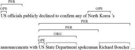
Figure 1: An example sentence in the ACE dataset with its nested entities. Viewing the nested entity structure as a partially observed tree, a key observation is that other spans without annotation can be modeled as latent nodes (dashed lines) in a full tree. This observation motivates us to model nested NER with partially-observed constituency trees.

Figure 1 gives an example sentence with nested entities. We observe that an inner entity can be part of an outer entity, which is quite similar to the constituency structure. Additionally, the boundaries of nested entities cannot cross. These observations motivate us to formulate nested NER as parsing with partially observed constituency trees: we can view entities with annotations as observed constituents, and assume a distribution of latent constituents over spans without annotation. For example, State Department and Richard Boucher can be two possible latent entities in Figure 1.

In this work, we propose to model observed and latent entities jointly with a TreeCRF (Zhang, Zhou, and Li 2020; Rush 2020). Specifically, we use a pretrained encoder to obtain word representations, a biaffine scoring mechanism (Dozat and Manning 2017) to obtain log potentials, and a TreeCRF to decode full constituency trees. Using TreeCRFs gives the advantage of modeling different types of entities in a probabilistically principled way and properly handling the ambiguities of the latent constituents. For optimization, we marginalize all latent constituents out, and maximize the resulting probability of observed partial trees.

Previously, the application of TreeCRFs for parsing is limited by the cubic time complexity of the Inside algorithm (Eisner 2016). Recent works show that it is possible to parallelize the Inside algorithm on modern hardware (Rush 2020). While a vanilla Inside algorithm sums over all possible trees, in our setting, we require an Inside-styled partial marginalization which only sums over latent nodes. To adapt the Inside algorithm to partial summation, we propose a masking method that differentiates different nodes during marginalization. Furthermore, to efficiently compute partial marginalization, we propose a Masked Inside algorithm that performs different inference operations for different types of nodes in a unified masked summation framework. We highlight the advantages of the Masked Inside compared with a naive partial marginalization algorithm from two perspectives: (a) it is highly batchifiable and parallelizable, allowing us to fully exploit the computational power of modern hardware (like GPUs) and tensor libraries (like Pytorch); (b) it is conceptually simple and can be easily implemented by reusing existing implementation of the original Inside algorithm in highly optimized structured prediction libraries (like Torch-Struct Rush 2020).

We further propose two regularization techniques for TreeCRFs. Specifically, we propose potential normalization, inspired by batch normalization (Ioffe and Szegedy 2015), and structure smoothing, inspired by label smoothing (Müller, Kornblith, and Hinton 2019). These two regularizations can be seamlessly integrated with Masked Inside, making their implementation simple and efficient.

We conduct experiments on three standard benchmark datasets. Experimental results show that our approach achieves 86.6, 85.4, and 78.2 scores in terms of F1 on the ACE2004, ACE2005, and GENIA datasets, respectively, which achieves SOTA F1 scores on the ACE2004, ACE2005 dataset, and shows comparable performance to SOTA models on the GENIA dataset. We will release the codes for further research. Our contributions are:

• We propose to formulate nested NER as constituency parsing with partial trees and use partially-observed TreeCRFs to jointly model observed and latent nodes.

• We propose the Masked Inside algorithm for efficient partial marginalization and its regularization techniques.

• We demonstrate the effectiveness of our proposed methods with extensive experiments.

Related Work

Nested NER

It has been a long history of research involving named entity recognition (Zhou and Su 2002; McCallum and Li 2003). In the era of deep learning, the LSTM-CRF model achieves very good results in recognizing named entities (Huang, Xu, and Yu 2015; Lample et al. 2016), especially when equipped with pretrained encoders (Peters et al. 2018; Devlin et al. 2019). Finkel and Manning (2009) point out that named entities are often nested while traditional sequential labeling models cannot handle the nested structure because they can only assign one label to each token. Earlier research on nested NER is rule-based (Zhang et al. 2004). Recent works in nested NER are in various paradigms as follows:

Hypergraph-based Lu and Roth (2015); Katiyar and Cardie (2018); Wang and Lu (2018) propose the hypergraph-based method to solve this problem. They design a hypergraph to represent all possible nested structures, which guarantees that nested entities can be recovered from the hypergraph tags. However, the hypergraph needs to be carefully designed to avoid spurious structures and structural ambiguities which inevitably leads to higher modeling and computational complexity. Compared with hypergraph-based approaches, our method tackles ambiguities in a probabilistically principled way by marginalizing all possible latent spans out, and can be implemented easily and efficiently.

Transition-based Transition-based models are generally similar to shift-reduce parsers with tailored actions for different formalisms. Wang et al. (2018) propose a method to construct nested mentions via a sequence of shift/ reduce/ unary actions. Fisher and Vlachos (2019) propose to form nested structures by merging tokens and/or entities into entities for entity representation. Compare with these methods, our approach does not involve the manual labor for designing specialized transition systems, which largely requires domain expertise thus being not generalizable. Our partially observed TreeCRFs is more general-purpose and can be flexibly applied to partial trees of different formalisms.

Span-based Another strategy for nested NER is the span-based methods (Xu, Jiang, and Watcharawittayakul 2017; Sohrab and Miwa 2018; Xia et al. 2019; Luan et al. 2019; Zheng et al. 2019; Tan et al. 2020; Jue et al. 2020). These models first compute the representations for all subsequences in a sentence with tailored neural architectures, then classify these spans with locally-normalized scores. Compared with these models, our TreeCRF can model the dependency for all subsequences with a globally-normalized structured distribution, which consequently leads to clear performance improvements.

Others There are many other attempts for Nested NER. Muis and Lu (2017) develop a gap-based tagging schema to capture nested structures. Lin et al. (2019) propose a sequence-to-nuggets architecture for nested mention detection. Straková, Straka, and Hajic (2019) propose to use a sequence-to-sequence framework to predict the entity label one by one. Li et al. (2020) treat NER as a machine reading comprehension task. Generally, it is hard to study nested NER in a unified framework and we aim to model it in a probabilistically principled way with TreeCRFs.

Constituency Parsing with TreeCRFs

TreeCRFs (Eisner 2000, 2016; Zhang, Zhou, and Li 2020) are well-studied in the parsing literature. Before the resurgence of deep learning, their application is limited due to its cubic time complexity. Recent work shows that with parallel computation (Zhang, Zhou, and Li 2020; Rush 2020), they can be efficiently implemented on modern hardware with high-optimized tensor operation libraries, reducing the complexity to at least quadratic time.

Traditional literature focus on parsing with full annotations. Although some works study partial annotation, many of them are limited in simulated datasets, e.g., by dropping out certain nodes from fully-annotated trees (Zhang et al. 2017; Zhang, Li, and Zhang 2020). Rather than being simulated, we emphasize that our application of TreeCRFs on Nested NER is a real-world example. Moreover, we note that our approach is not limited to nested NER, and an interesting future direction would be applying it for parsing with other types of partial trees.

Model

Our model consists of a pretrained encoder, a biaffine scoring module, and a TreeCRF model. Given a sentence, we obtain the contextualized representations from the encoder, feed the representations to the biaffine layer to get the log potentials for the TreeCRF model, then use the TreeCRF to decode a constituency tree. To calculate the probability of partial trees, we propose the Masked Inside algorithm as a simple, efficient algorithm for partial marginalization.

The Base Biaffine Scoring Architecture

Given a sentence $x$ as a sequence of words: $x=[x_{1},x_{2},...,x_{n}],x_{i}\in\mathcal{V}$, $\mathcal{V}$ is the vocabulary and $n$ is the sentence length. We use a base biaffine encoder similar to the biaffine dependency parser in Dozat and Manning (2017) to predict span scores:

$$e_{1},...,e_{n} =\text{FF}(\text{Enc}(x))$$ (1)

$$s_{ijk} =e_{i}^{\intercal}U_{k}^{(1)}e_{j}+(e_{i}+e_{j})^{\intercal}U_{k}^{(2)}+b_{k}$$ (2)

Where Enc$(\cdot)$ denotes a pretrained encoder, FF$(\cdot)$ denotes a feed-forward network, $e_{i}$ denotes the contextualized embedding for word $x_{i}$, $U_{k}^{(1)}$, $U_{k}^{(2)}$ and $b_{k}$ are the parameters for the biaffine scoring mechanism, and $s_{ijk}$ means the score for a constituent spanning from word $x_{i}$ to $x_{j}$ (inclusive) with label $k$ where $i,j\in[1,2,...,n],k\in[1,2,...,|\mathcal{L}|]$, $\mathcal{L}$ is the set of labels for the constituents. We further note $\mathcal{L}$ is a union of observed labels $\mathcal{L}_{o}$ and latent labels $\mathcal{L}_{l}$, as we will explain later.

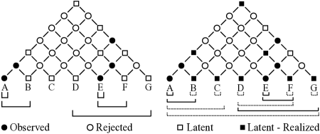
Figure 2: An example symbol tree. Left: observed partial tree (lower) and its corresponding symbol tree (upper) with different types of nodes induced from the observed tree. The symbol tree notation further enables us to build different types of masks for the Masked Inside algorithm. Right: a full tree compatible with the left partial tree (lower) by realizing the latent nodes from

$\square$

to

$\blacksquare$

(upper). An entity with dashed lines corresponds to a realized latent node

$\blacksquare$

. A partial tree may correspond to different realized full trees.

Partially-Observed TreeCRFs

A constituency TreeCRF is a probabilistic discriminative model that defines a distribution over constituency trees $T$ given sentence $x$. We represent a labeled constituency tree as a rank-3 binary tensor $T$ where $T_{ijk}=1$ means that there is a span from word $x_{i}$ to $x_{j}$ with label $k$. We use the biaffine scores $s_{ijk}$ as the log potentials, and the probability of a tree is given by the Gibbs distribution:

$$s(T) =\sum_{ijk}T_{ijk}s_{ijk}$$ (3)

$$p(T|x) =\frac{\exp(s(T))}{Z}$$ (4)

$$Z =\sum_{T}\exp(s(T))=\textsc{Inside}(s)$$ (5)

Where $Z$ is the partition function that sums over all possible tree structure $T$, which can be computed exactly with the Inside algorithm (Eisner 2016).

For nested NER, the annotations of trees are incomplete so we only get partial trees. With a slight abuse of notation, we still use $T$ to denote partial trees, and there are locations in $T$ that might be 1 but filled in with 0 because it is not observed (latent). To better understand the nature of different nodes in a partial tree, we introduce a convenient symbol tree notation $\bar{T}$ given a partial tree $T$. $\bar{T}$ is a $n\times n$ matrix with difference types of nodes. Algorithm 1 gives details for building symbol trees $\bar{T}$ (we delay the discussion about the mask $M$ returned from Algorithm 1 to the next section). Nodes in $\bar{T}$ can only be one of $\bullet$, $\square$ or $\circ$. Figure 2 left gives an example of $\bar{T}$. A $\bullet$ in $\bar{T}$ means an observed node (a labeled entity) in $T$, a $\circ$ means a node that is incompatible with observed nodes because it overlaps with an observed entity (e.g., there cannot be a latent entity [BC] because B is already in the observed entity [AB] and the boundaries of entities cannot cross) and a $\square$ means a latent node that is possible to be realized in a full tree (e.g., there is a possible entity [ABC] with some latent label). We note leaf nodes and the root can only be observed $\bullet$ or latent $\square$ .

Algorithm 1 Symbol Tree and Mask Construction

1:Input: partial tree $T$, $\mathcal{L}_{o}$ observed labels, $\mathcal{L}_{l}$ latent labels.

2:$\triangleright$ Initialize all nodes as latent

$\square$

:

3: For all $i,j\in\{1,2,...,n\}$: $\bar{T}[i,j]=\text{\scalebox{0.8}{$\square$}}$ $\forall k_{1}\in\mathcal{L}_{o},M[i,j,k_{1}]=0;\;\;\;\forall k_{2}\in\mathcal{L}_{l},M[i,j,k_{2}]=1$

4:for $i,j\leftarrow 1$ to $n$ do

5:     if $\exists k,T_{ijk}=1$ then $\triangleright$ Observe entity $(i,j)$ with label $k$

6:         $\bar{T}[i,j]=\bullet$

7:         $M[i,j,k]=1$, $\forall m\in\mathcal{L},m\neq k,M[i,j,m]=0$

8:         $\triangleright$ For all spans with crossed boundaries with $(i,j)$:

9:          $\forall(i^{\prime},j^{\prime}),i^{\prime}<i\;\&\;i\leq j^{\prime}<j$: $\bar{T}[i^{\prime},j^{\prime}]=\circ,\;\;\forall m\in\mathcal{L},M[i^{\prime},j^{\prime},m]=0$

10:          $\forall(i^{\prime},j^{\prime}),i<i^{\prime}\leq j\;\&\;j<j^{\prime}$: $\bar{T}[i^{\prime},j^{\prime}]=\circ,\;\;\forall m\in\mathcal{L},M[i^{\prime},j^{\prime},m]=0$      

11:Return: symbol tree $\bar{T}$, mask $M$

Given the partial tree $T$, a full tree $\tilde{T}$ compatible with $T$ can be constructed by realizing $\square$ to $\blacksquare$ in $\bar{T}$ (Figure 2 right. A $\blacksquare$ in the upper part denotes a realized latent span corresponding to an entity with a dashed line in the lower part). We further denote the set of labels for latent spans $\mathcal{L}_{l}$ as opposed to the labels for observed entities $\mathcal{L}_{o}$. We restrict the labels for the latent spans to be within $\mathcal{L}_{l}$. For example, the labels for the constituents [ABC] and [DEF] are only allowed to be in $\mathcal{L}_{l}$ because they are latent. This separation would allow us to decode partial trees during inference by dropping out entities with latent labels. Since there are multiple ways to complete a partial tree, we use $\tilde{\mathcal{T}}$ to denote the set of full trees completed from $T$.

To train the TreeCRF with partial trees, we maximize the conditional probability of $p(T|x)$ computed by marginalizing all latent nodes $\square$ out:

$$\log p(T|x)=s(T)-\log Z$$ (6)

$$s(T)=\log\sum_{\tilde{T}\in\tilde{\mathcal{T}}}\exp(s(\tilde{T}))$$ (7)

This objective could equivalently be viewed as the average probability of the observed partial tree $T$ over its all possible compatible full trees in $\tilde{\mathcal{T}}$.

Algorithm 2 Inside for Partial Marginalization

1:Input: Scores $s$, partial tree $T$ and its corresponding $\bar{T}$

2:for $i\leftarrow 1$ to $n$ do

3:     if $\bar{T}[i,i]=\bullet$ then $\triangleright$ Observed leaf

4:         $\exists k\in\mathcal{L}_{o},T_{iik}=1,\beta[i,i,k]=\exp(s_{iik})$

5:         $\forall m\neq k,\beta[i,i,m]=0$

6:     else if $\bar{T}[i,i]=\text{\scalebox{0.8}{$\square$}}$ then $\triangleright$ Latent leaf

7:         $\forall k\in\mathcal{L}_{o},\beta[i,i,k]=0$

8:         $\forall k\in\mathcal{L}_{l},\beta[i,i,k]=\exp(s_{iik})$      

9:for $d\leftarrow 1$ to $n-1$ do

10:     for $i\leftarrow 1$ to $n-d$ do

11:         $j=i+d$

12:         if $\bar{T}[i,j]=\bullet$ then $\triangleright$ Observed

13:              $\exists k\in\mathcal{L}_{o},T_{ijk}=1$

14:               $\beta[i,j,k]=\exp(s_{ijk})\cdot$ $\sum_{l=i}^{j-1}\sum_{k_{1},k_{2}\in\mathcal{L}}\beta[i,l,k_{1}]\beta[l+1,j,k_{2}]$

15:              $\forall m\neq k,\beta[i,j,m]=0$

16:         else if $\bar{T}[i,j]=\text{\scalebox{0.8}{$\square$}}$ then $\triangleright$ Latent

17:               $\forall k\in\mathcal{L}_{l},\beta[i,j,k]=\exp(s_{ijk})\cdot$ $\sum_{l=i}^{j-1}\sum_{k_{1},k_{2}\in\mathcal{L}}\beta[i,l,k_{1}]\beta[l+1,j,k_{2}]$

18:              $\forall k\in\mathcal{L}_{o},\beta[i,j,k]=0$

19:         else if $\bar{T}[i,j]=\circ$ then $\triangleright$ Rejected

20:              $\forall k\in\mathcal{L},\beta[i,j,k]=0$               

21:if $\bar{T}[1,n]=\bullet$ then $\triangleright$ Observed root

22:     $\exists k\in\mathcal{L}_{o},T_{1nk}=1$. Return $s(T)=\beta[1,n,k]$

23:else if $\bar{T}[1,n]=\text{\scalebox{0.8}{$\square$}}$ then $\triangleright$ Latent root

24:     Return $s(T)=\log(\sum_{k\in\mathcal{L}_{l}}\beta[1,n,k])$

Masked Inside for Efficient Partial Marginalization

To compute the partial marginalization in equation (7), we give a tailored Inside algorithm that supports different inference operations for different nodes. As is shown in Algorithm 2, during the summation process, if the current node is: (a) an observed $\bullet$, then we evaluate (add) its corresponding score (line 4 and 14); (b) a latent  $\square$ whose label can only be in $\mathcal{L}_{l}$. So we reject (do not add) all the scores corresponding to observed labels $\mathcal{L}_{o}$ (line 7 and 18), and sum over all scores corresponding to latent labels $\mathcal{L}_{l}$ for this node (line 8 and 17); (c) a rejected $\circ$, we reject all scores corresponding to this node (line 20).

However, a naive implementation of Algorithm 2 can be inefficient with $O(n^{3})$ complexity. Such inefficiency has previously restricted the application of TreeCRFs in parsing literature. More severely, Algorithm 2 does not support batch computation over sentences, making it more impractical. Recent works show that, for the original Inside algorithm, it is possible to parallelize it on modern hardware architectures with efficient batch computation, reducing the complexity from $O(n^{3})$ to at least $O(n^{2})$, and could further be $O(n\log n)$ (Rush 2020; Zhang, Zhou, and Li 2020). It would be ideal if we could use similar batchification techniques for Algorithm 2, which motivates our proposed Masked Inside algorithm for efficient partial marginalization.

Algorithm 3 Masked Inside

1:Input: Scores $s$, mask $M$

2:for $i\leftarrow 1$ to $n$ do

3:     $\beta[i,i,k]=M[i,i,k]\cdot\exp(s_{iik})$ $\triangleright$ Masked leaf scores

4:for $d\leftarrow 1$ to $n-1$ do

5:      Parallelization on $i$, tensor operation on $l,k,k_{1},k_{2}$ $1\leq i\leq n-d$; $\;\;j=i+d$; $\;\;k,k_{1},k_{2}\in\{1,...,|\mathcal{L}|\}$

6:      $\beta[i,j,k]=(M[i,j,k]\exp(s_{ijk}))\;\cdot$ $\triangleright$ Masked scores $\sum_{l=i}^{j-1}\sum_{k_{1},k_{2}\in\mathcal{L}}\beta[i,l,k_{1}]\beta[l+1,j,k_{2}]$

7:Return: $s(T)=\log(\sum_{k\in\mathcal{L}}\beta[1,n,k])$

As is shown in Algorithm 3, the key insight of Masked Inside is that all if-else statements for partial summation in Algorithm 2 can be re-written in a unified masked summation (line 3 and 6 in Algorithm 3) with a pre-computed mask $M$ from Algorithm 1. To be specific, in Algorithm 1: (a) for an observed node $\bullet$, we mask out all scores except the score of its observed label (line 7), which corresponds to lines 4, 14 and 21 in Algorithm 2; (b) for a rejected node $\circ$, we mask out all its scores (lines 9-10), which corresponds to line 19 in Algorithm 2; (c) for a latent node  $\square$ , we mask out the scores for all observed labels $\mathcal{L}_{o}$, and retain scores for all latent labels $\mathcal{L}_{l}$ (line 3), which corresponds to lines 6, 16, and 23 in Algorithm 2. Applying different masks to Algorithm 3, we can recover all if-else statements in Algorithm 2. As two special cases, if all masks are 1 (i.e., not masked), we recover the original Inside algorithm; if the masks are constructed from a full tree, we recover the original bottom-up evaluation.

	ACE2004			ACE2005			GENIA
	Train	Dev	Test	Train	Dev	Test	Train	Dev	Test
# sentences	7,078	859	922	7,194	969	1,047	14,836	1,855	1,855
with nested entities	2,691	290	377	2,691	338	330	3,199	362	448
# entities	22,172	2,510	3,024	24,441	3,200	2,993	46,473	5,014	5,600
# nested entities	10,080	1,086	1,410	9,389	1,112	1,118	8,337	903	1,217
avg length	20.38	20.69	20.96	19.21	18.93	17.19	30.13	29.17	30.48

Table 1: Statistics of ACE2004, ACE2005, and GENIA datasets.

	ACE2004			ACE2005			GENIA
Model	P	R	F1	P	R	F1	P	R	F1
LSTM-CRF (Lample et al. 2016)	71.3	50.5	58.3	70.3	55.7	62.2	75.2	64.6	69.5
FOFE(c=6) (Xu et al. 2017)	68.2	54.3	60.5	76.5	66.3	71.0	75.4	67.8	71.4
Transition (Wang et al. 2018)	74.9	71.8	73.3	74.5	71.5	73.0	78.0	70.2	73.9
Cascaded-CRF (Ju et al. 2018)	-	-	-	74.2	70.3	72.2	78.5	71.3	74.7
SH(c=n) (Wang and Lu 2018)	77.7	72.1	74.5	76.8	72.3	74.5	77.0	73.3	75.1
ML (Fisher and Vlachos 2019)	-	-	-	75.1	74.1	74.6	-	-	-
BENSC (Tan et al. 2020)	78.1	72.8	75.3	77.1	74.2	75.6	78.9	72.7	75.7
Pyramid (Jue et al. 2020)	81.1	79.4	80.3	80.0	78.9	79.4	78.6	77.0	77.8
with Pretrained LM
MGNER (ELMo) (Xia et al. 2019)	81.7	77.4	79.5	79.0	77.3	78.2	-	-	-
ML (ELMo) (Fisher and Vlachos 2019)	-	-	-	79.7	78.0	78.9	-	-	-
ML (BERT) (Fisher and Vlachos 2019)	-	-	-	82.7	82.1	82.4	-	-	-
Seq2seq (Straková, Straka, and Hajic 2019)	-	-	84.3	-	-	83.4	-	-	78.2
BENSC (BERT) (Tan et al. 2020)	85.8	84.8	85.3	83.8	83.9	83.9	79.2	77.4	78.3
Pyramid (BERT) (Jue et al. 2020)	86.1	86.5	86.3	84.0	85.4	84.7	79.5	78.9	79.2
with Additional Supervision
DYGIE (Luan et al. 2019)	-	-	84.7	-	-	82.9	-	-	76.2
Yu, Bohnet, and Poesio (2020)	87.3	86.0	86.7	85.2	85.6	85.4	81.8	79.3	80.5
BERT-MRC (Li et al. 2020)	85.0	86.3	86.0	87.2	86.6	86.9	85.2	81.1	83.8
PO-TreeCRFs (ours)	86.7	86.5	86.6	84.5	86.4	85.4	78.2	78.2	78.2
	$\pm$0.4	$\pm$0.4	$\pm$0.3	$\pm$0.4	$\pm$0.2	$\pm$0.1	$\pm$0.7	$\pm$0.8	$\pm$0.1
PO-TreeCRFs Ablation Study
Change Biaffine to Bilinear	86.0	86.7	86.4	83.0	86.5	84.7	79.9	75.5	77.6
W/o. Structure Smoothing	86.1	86.4	86.2	83.5	85.8	84.6	78.7	76.5	77.6
W/o. Potential Normalization and Structure Smoothing	86.0	85.3	85.7	82.7	86.2	84.4	76.5	78.1	77.3
W/o. TreeCRFs	84.4	85.4	84.9	82.0	86.4	84.1	80.5	74.5	77.4

Table 2: Main results and ablation studies on three datasets. We report the average scores of 5 runs for main results.

As an efficient alternative for Algorithm 2, the advantages of Algorithm 3 is that it is (a) conceptually much simpler and (b) highly parallelizable. The later allows us to fully exploit the computational power of modern hardware architectures (like GPUs) and highly optimized tensor operation libraries (like Pytorch). We note that it the parallelization on $i$ in Algorithm 3 that reduces the complexity to at least $O(n^{2})$, Furthermore, as an equivalent implementation to Algorithm 3, we can apply masks to scores in the logarithm scale then feed the masked scores to a normal Inside algorithm (rather than multiplying the masks inside Algorithm 3):

$$s(T) =\textsc{MaskedInside}(s,M)$$

$$=\textsc{Inside}(\log M+s)$$ (8)

$$p(T|x) =\frac{\exp(s(T))}{Z}$$ (9)

In practice, we compute the masks $M$ in the data-processing stage. For training, by reusing existing implementations of the Inside algorithm in highly-optimized structured prediction libraries like Torch-Struct (Rush 2020), we can implement the Masked Inside with one single line of code, as is shown in equation (8), thus significantly reducing the implementation complexity required by Algorithm 2.

Regularization

We propose two regularization techniques for TreeCRFs: (a) potential normalization, which is inspired by batch normalization (Ioffe and Szegedy 2015), and (b) structure smoothing, which is inspired by label smoothing (Müller, Kornblith, and Hinton 2019). Potential normalization (PN) is simple: we normalize the scores $s$ to an empirical distribution of zero mean and one variance. The difference with batch-norm (BN) is that we apply PN at an instance-level, rather than a batch-level. In our experiments, we observe that PN gives a slightly better convergence.

Structure smoothing regularizes TreeCRFs by putting a small portion of weights to nodes that are marginalized out. Specifically, during the partial marginalization, instead of using a zero mask that does not include the weights of rejected nodes, we change the mask to a small value $\epsilon$

$$M[i,j,k]=0\to M[i,j,k]=\epsilon\quad\text{for rejected $\circ$}$$ (10)

This would effectively add the weights of all rejected nodes to $s(T)$ with a multiplier $\epsilon$. This is similar to label smoothing which adds a small portion of weights to all labels other than the target label. The reason that we call it structure smoothing is that it not only smooths over the labels, but also smooths over different tree structures. We further observe that structure smoothing should be based on potential normalization for numerical stability, otherwise it does not converge in our experiments. The implementation of structure smoothing is still easy and aligns with previous discussions about equation (8) as one only needs to change the zeros in $M$ to $\epsilon$.

Training and Inference

During training, we maximize the log conditional probability $\log p(T|x)$ efficiently computed by equation (8) and (9). During inference, we use CKY decoding to decode a full tree with the maximum probability. We only include nodes whose labels are in the observed label set $\mathcal{L}_{o}$, and dismiss nodes whose labels are in the latent set $\mathcal{L}_{l}$. This would allow us to decode nested entities (partial trees) for evaluation.

Experiments

We conduct experiments on three standard benchmark datasets. We show that our proposed approach achieves SOTA performance. We further conduct detailed error analysis, case study, and time complexity analysis.

Datasets

We conduct experiments on the ACE2004, ACE2005 (Doddington et al. 2004), and GENIA (Kim et al. 2003) datasets. There are seven types of entities as ‘FAC’, ‘LOC’, ‘ORG’, ‘PER’, ‘WEA’, ‘GPE’, ‘VEH’ in the ACE datasets and five types of entities as ‘G#DNA’, ‘G#RNA’, ‘G#protein’, ‘G#cell_line’, ‘G#cell_type’ in the GENIA dataset. The statistics of these datasets are shown in Table 1.

Implementation Details

We use variants of BERT (Devlin et al. 2019) to encode sentences. For the ACE2004 and ACE2005 datasets, we use the bert-large-cased checkpoint. For GENIA, we use BioBERT v1.1 (Lee et al. 2020). As words in the sentence are divided into word pieces, we use the representation of the first piece to represent each word after BERT encoding. The parameter in BERT is also trainable. We use AdamW optimizer with the learning rate 2e-5 on ACE2004 dataset and 3e-5 on ACE2005 and GENIA dataset. The $\epsilon$ used for structure smoothing is 0.01 on ACE2004 dataset and 0.02 on ACE2005 and GENIA dataset. We apply 0.2 dropout after BERT encoding. Denote the hidden size of the encoder as $h$ ($h=1024$ for BERT Large, and $768$ for BioBERT). We apply two feed-forward layers before the biaffine scoring mechanism, with $h$ and $h/2$ hidden size, respectively. Consequently, the size of biaffine matrix is $h/2\times h/2$. We set the size of latent labels $\mathcal{L}_{l}$ to 1 as in our preliminary experiments we find out the performance does not differ significantly with more latent labels.

Baselines

Below we list our baseline models with comparable settings. We also include the results of models that use additional supervision, which are not directly comparable to ours.

LSTM-CRF

is a classical baseline for NER. This model cannot solve the problem of nested entities (Lample et al. 2016).

FOFE

is a span-based method that classifies over all sub-sequences of a sentence with a fixed-size forgetting encoding (Xu, Jiang, and Watcharawittayakul 2017).

Transition

is a shift-reduce based system that learns to construct the nested structure in a bottom-up manner through an action sequence (Wang et al. 2018).

Cascaded-CRF

applies several stacked CRF layers to recognize nested entities at different levels in an inside-out manner (Ju, Miwa, and Ananiadou 2018).

SH

improves LH (Katiyar and Cardie 2018) by considering the transition between labels to alleviate labeling ambiguity of hypergraphs (Wang and Lu 2018).

MGNER

first applies the Detector to generate possible spans as candidates and then applies a Classifier for the entity type (Xia et al. 2019).

Merge and Label (ML)

first merges tokens and/or entities into entities forming nested structures and then labels entities to corresponding types (Fisher and Vlachos 2019).

Seq2seq

is under a encoder-decoder framework to predict the entity one by one (Straková, Straka, and Hajic 2019).

BENSC

is a span-based method that incorporates a boundary detection task for multitask learning (Tan et al. 2020).

Pyramid

is the state-of-the-art method without external supervision. It recursively inputs tokens and regions into flat NER layers for span representations (Jue et al. 2020).

Figure 3: Inferred latent tree structure examples. Solid lines: predicted entities; dashed lines: realized latent constituents. Although there are spans that are not that meaningful like rights group, we still observe meaningful inferred spans like for strategic and international studies and in Jakarta.

Results

Table 2 shows the overall results on ACE2004, ACE2005, and GENIA. We primarily compare our model with the Pyramid(BERT) model (Jue et al. 2020), as it achieves SOTA scores without additional supervision signals. As we believe there are still rooms for further performance improvements, e.g., to use a more powerful, larger encoder (like GPT3 Brown et al. 2020) or to use more ensemble methods, e.g., to ensemble FLAIR (Akbik, Blythe, and Vollgraf 2018) and other pretrained encoders, to standardize the comparison and validate the effectiveness of TreeCRFs, we restrict the encoder to be BERT. We denote our partially-observed TreeCRF as PO-TreeCRF. Our PO-TreeCRF achieves 86.6, 85.4, and 78.2 scores in terms of $F_{1}$ on the ACE2004, ACE2005, and GENIA datasets, respectively, which achieves the state of the art F1 scores on the ACE2004, ACE2005 dataset, and shows comparable performance to Pyramid(BERT) on the GENIA dataset.

We further emphasize the evaluation of nested NER is not strictly standardized and there are more or less differences across different works. As is in Table 2, there are models that show improvements with additional information. Specifically, DYGIE (Luan et al. 2019) uses the OntoNotes annotations for better coreference resolution. Yu, Bohnet, and Poesio (2020) train and evaluate their model at the paragraph level which gives a better coreference resolution performance. Their work is under a different setting as the training and evaluation of most works are at the sentence level. BERT-MRC (Li et al. 2020) takes annotation guideline notes as references to construct queries, which is strong supervision and the corresponding corpus are not always easy to obtain. As we try to align our evaluation with the majority of literature, the models mentioned above are not directly comparable to our method.

	PER	LOC	ORG	GPE	FAC	VEH	WEA
$\rho$	0.58	0.02	0.17	0.14	0.05	0.03	0.02
PER	0.93	0.00	0.07	0.05	0.01	0.03	0.00
LOC	0.00	0.72	0.00	0.02	0.05	0.00	0.00
ORG	0.02	0.02	0.77	0.00	0.02	0.01	0.00
GPE	0.00	0.06	0.03	0.84	0.03	0.00	0.00
FAC	0.00	0.02	0.01	0.00	0.70	0.03	0.00
VEH	0.00	0.00	0.00	0.00	0.01	0.67	0.00
WEA	0.00	0.00	0.00	0.00	0.00	0.01	0.84
Latent	0.02	0.15	0.08	0.05	0.12	0.15	0.10
None	0.03	0.04	0.04	0.03	0.06	0.10	0.06

Table 3: Error distribution on ACE2005. Rows: entities predicted by our model. None denotes the entities that are not predicted. Columns: labeled entities. Numbers are normalized by columns. $\rho$ denotes the prior distribution of labels.

Ablation Study

Table 2 lowest rows show the results of ablation study. We note that structure smoothing should be based on potential normalization otherwise the model does not converge. By without TreeCRFs we mean to use the biaffine scorer and normalize the scores locally, similar to Yu, Bohnet, and Poesio (2020). Not using TreeCRFs would lead to the largest performance drop which demonstrates the effectiveness of global normalization with TreeCRFs. We also observe performance drop when we do not use potential normalization and structure smoothing which validates their effectiveness for regularizing TreeCRFs.

Error Analysis

In our experiments, we find out the recall for unlabeled spans is 96.3 on ACE2005, which means that the spans for most entities are correctly covered, and it is their labels that are more difficult to predict. To see which labels are more prone to errors, we report the error distribution in Table 3. We see that the VEH, FAC, and LOC are the top three classes prone to errors as they are extremely imbalanced (0.03, 0.05, and 0.02 respectively), and many of them are predicted as latent. This indicates that a future direction is to adapt the TreeCRF to imbalanced labels. We leave it to future work.

Case Study

Figure 3 gives examples of inferred latent tree structures compatible with predicted entities. As the learning of latent structures is completely unsupervised, we may not expect that the inferred subtrees should align with human intuition, and we do observe some spans that are not that interpretable like rights group. However, we still observe some meaningful constituents like for strategic and international studies and in Jakarta, which indicates that our approach is indeed learning meaningful tree structures to a certain extent. We note there are also related unsupervised grammar induction works with TreeCRFs (Kim et al. 2019; Kim, Dyer, and Rush 2019), and we leave the application of our model to grammar induction to future work.

Method	Inside (Vanilla)	Masked Inside	Biaffine
GPU Time	14m58s	3m20s	2m27s
CPU Time	2h5m	24m	22m10s
Complexity	$O(n^{3})$	$O(n\log n)$	$O(1)$

Table 4: Time for training one epoch on ACE2004. GPU Nvidia P100, CPU Intel 2.6Hz quad-core i7.

Time Complexity

Table 8 shows the speed for training different models. We primarily focus on GPU time, but also report CPU time. The base Biaffine model is similar to the model in Yu, Bohnet, and Poesio (2020) which uses locally normalized scores, instead of using a TreeCRF. This model eliminates the complexity of the Inside algorithm and can be computed in $O(1)$ time. which can be viewed as an upper bound of time complexity. Thanks to the masking mechanism that is compatible with parallelization and tensor operations, our Masked Inside is significantly quicker than a vanilla implementation of Inside for partial marginalization, and is close to the base Biaffine in practice.

Conclusion

In this work, we propose to view nested entity structures as partially observed constituency trees, and model it with partially observed TreeCRFs. We use a pretrained encoder and a biaffine scoring module to predict the log potentials, then use the TreeCRF to decode the entities. We give a detailed discussion of different nodes within partial trees and their corresponding inference operations during partial marginalization. To facilitate efficient computation with modern hardware and tensor libraries, we propose the Masked Inside algorithm that is conceptually simple and practically efficient. We demonstrate the effectiveness and efficiency of our approach with extensive experiments.

Appendix A Appendix

	ACE2004			ACE2005			GENIA
	P	R	F1	P	R	F1	P	R	F1
Run 1	86.94	86.20	86.57	84.82	86.33	85.57	77.31	79.31	78.29
Run 2	86.92	86.63	86.77	84.80	86.42	85.61	78.92	77.58	78.24
Run 3	86.83	85.97	86.40	83.92	86.76	85.31	77.96	78.39	78.17
Run 4	86.14	86.63	86.38	84.16	86.52	85.33	77.85	78.62	78.24
Run 5	87.03	87.09	87.06	84.62	86.09	85.35	79.00	77.29	78.14

Table 5: Detailed Results of 5 Runs. The numbers does not vary much, which means that our model performance is not sensitive to random initialization.

	ACE2004			ACE2005			GENIA
# Latent Labels	P	R	F1	P	R	F1	P	R	F1
1	86.7	86.5	86.6	84.5	86.4	85.4	78.2	78.2	78.2
2	86.5	86.0	86.3	84.1	86.9	85.1	76.6	79.9	78.2
3	86.2	86.9	86.6	83.0	87.4	85.1	77.7	78.1	77.9
4	85.6	86.6	86.1	83.1	86.8	84.9	75.2	80.2	77.6
5	84.8	88.1	86.4	83.7	86.9	85.3	-	-	-
6	84.9	87.4	86.1	82.6	87.8	85.1	-	-	-
label size	84.3	87.4	85.8	82.6	87.5	85.0	76.7	77.6	77.2
2 * label size	84.2	87.5	85.8	82.6	87.0	84.7	77.0	76.7	76.9
3 * label size	83.5	87.4	85.4	82.3	86.5	84.3	76.6	77.3	77.0

Table 6: Results of varying the number of latent labels $|\mathcal{L}_{l}|$ on the ACE2004, ACE2005, and GENIA dataset. The observed label size is 7 in ACE2004 and ACE2005 datasets, and 5 in GENIA dataset. As the size of the latent labels increases, we observe an interesting trend of increasing recall and decreasing precision. This means that the model is making more radical predictions, targeting on coverage (recall) rather than confidence (precision). See the corresponding paragraph for detailed discussions.

Method	UAS
Random	10.83
Left-branching	5.61
Right-branching	0.15
PO-TreeCRF (ours)	16.95
Oracle	78.51

Table 7: Alignment to syntactical constituency trees. Oracle trees are obtained by using CoreNLP to parse the sentences, then left-binarized to CNF. All the reported methods align poorly to the syntactical constituency trees, however, our method still gives higher UUAS than all baseline, meaning that a small fraction of tree structures predicted by our model are aligned with the syntactical structures.

Method	Masked Inside	Vanilla Partial Marginalization
GPU Time	3m20s	8m10s
CPU Time	24m	26m

Table 8: Time for training one epoch on ACE2004. GPU Nvidia P100, CPU Intel 2.6Hz quad-core i7. The vanilla partial marginalization algorithm does not support sentence batchification since different sentences have different tree structures, thus being significantly slower than the masked inside.

Detail Results of 5 Runs

Table 5 gives the full results of all 5 runs. We report the results simply to check if the model is sensitive to random seeds. The numbers show that the F1 scores do not vary much with different initialization, which means that the model is consistent under random initialization.

Number of Latent Labels

Table 6 shows the performance change as we increase the number of latent states. When the number of latent states is relatively small (less than 5), the performance does not vary much. So we report the performance for 1 latent state in the main paper. We also note that when we increase the number of latent states to be larger than the number of observed states, the performance drops significantly.

Table 6 shows an interesting trend of changing the size of latent labels: as we increase the number of latent labels, the precision is gradually decreasing while the recall is gradually increasing. To explain this observation, we make the following conjecture: (a) the sum of the prior probability of observed labels and latent labels is 1, and the prior probability of observed labels is fixed in the training set, so different latent labels would share the rest prior probability; (b) as the number of latent labels increases, each latent label would in average receive less probability; (c) during CKY decoding, since the probability of each latent label decreases on average, it is more likely that a tree involving more observed labels would be of higher probability, resulting the algorithm to decode out trees with more observed labels; (d) consequently, the model makes more radical predictions, leading to higher coverage of entities (higher recall) but lower precision. We note this reasoning chain is only a rough sketch, and we have not yet able to investigate the detailed mechanism. We leave it to future work.

Alignment to Syntax Trees

We further compare the trees inferred by our model with the syntactical constituency trees of the same sentence. We use unlabeled attachment score (UAS) as the similarity metric. We report the similarity on the training set. Specifically, we use Stanford CoreNLP to obtain the oracle constituency trees of the training sentences, binarize these trees to CNF using an always-left strategy. The UAS of the oracle trees means the similarity between the left-binarized oracle trees to the original oracle trees. We compare: (a) random trees (b) left-branching trees (d) right-branching trees (d) trees inferred from our NER model to the oracle trees. All baseline trees align poorly to the oracle constituency trees, while ours have the highest UAS. We emphasize that our trees are trained under a NER objective, and do not necessarily need to be similar to syntax trees. However, there is still a fraction of the tree structures inferred from our model that is similar to the syntactical constituency structures. We leave further investigation about the relationship between our latent trees and syntactical constituency trees to future work.

Batchification Speed with Masked Inside

We note that the vanilla partial marginalization algorithm (Algorithm 2) in the main paper does not support sentence-level bachification because different sentences have different tree structures. This inefficiency is addressed by the Masked Inside algorithm. To see how sentence-level batchification leads to further speed improvement, we report the speed comparison in Table 8. Generally, Masked Inside is significantly faster than a vanilla partial marginalization algorithm.

References

- Akbik, Blythe, and Vollgraf (2018) Akbik, A.; Blythe, D.; and Vollgraf, R. 2018. Contextual String Embeddings for Sequence Labeling. In Proceedings of the 27th International Conference on Computational Linguistics, 1638–1649. Santa Fe, New Mexico, USA: Association for Computational Linguistics. URL https://www.aclweb.org/anthology/C18-1139.
- Alex, Haddow, and Grover (2007) Alex, B.; Haddow, B.; and Grover, C. 2007. Recognising nested named entities in biomedical text. In Proceedings of the Workshop on BioNLP 2007: Biological, Translational, and Clinical Language Processing, 65–72.
- Brown et al. (2020) Brown, T.; Mann, B.; Ryder, N.; Subbiah, M.; Kaplan, J.; Dhariwal, P.; Neelakantan, A.; Shyam, P.; Sastry, G.; Askell, A.; Agarwal, S.; Herbert-Voss, A.; Krüger, G.; Henighan, T.; Child, R.; Ramesh, A.; Ziegler, D.; Wu, J.; Winter, C.; Hesse, C.; Chen, M.; Sigler, E.; Litwin, M.; Gray, S.; Chess, B.; Clark, J.; Berner, C.; McCandlish, S.; Radford, A.; Sutskever, I.; and Amodei, D. 2020. Language Models are Few-Shot Learners. ArXiv abs/2005.14165.
- Devlin et al. (2019) Devlin, J.; Chang, M.-W.; Lee, K.; and Toutanova, K. 2019. BERT: Pre-training of Deep Bidirectional Transformers for Language Understanding. In Proceedings of the 2019 Conference of the North American Chapter of the Association for Computational Linguistics, 4171–4186.
- Doddington et al. (2004) Doddington, G. R.; Mitchell, A.; Przybocki, M. A.; Ramshaw, L. A.; Strassel, S. M.; and Weischedel, R. M. 2004. The Automatic Content Extraction (ACE) Program-Tasks, Data, and Evaluation. In Lrec, volume 2, 1.
- Dozat and Manning (2017) Dozat, T.; and Manning, C. D. 2017. Deep Biaffine Attention for Neural Dependency Parsing. ICLR .
- Eisner (2000) Eisner, J. 2000. Bilexical Grammars and their Cubic-Time Parsing Algorithms.
- Eisner (2016) Eisner, J. 2016. Inside-Outside and Forward-Backward Algorithms Are Just Backprop (tutorial paper). In SPNLP@EMNLP.
- Finkel and Manning (2009) Finkel, J. R.; and Manning, C. D. 2009. Nested named entity recognition. In Proceedings of the 2009 Conference on Empirical Methods in Natural Language Processing, 141–150.
- Fisher and Vlachos (2019) Fisher, J.; and Vlachos, A. 2019. Merge and Label: A Novel Neural Network Architecture for Nested NER. In Proceedings of the 57th Conference of the Association for Computational Linguistics, 5840–5850.
- Huang, Xu, and Yu (2015) Huang, Z.; Xu, W.; and Yu, K. 2015. Bidirectional LSTM-CRF models for sequence tagging. arXiv preprint arXiv:1508.01991 .
- Ioffe and Szegedy (2015) Ioffe, S.; and Szegedy, C. 2015. Batch Normalization: Accelerating Deep Network Training by Reducing Internal Covariate Shift. In International Conference on Machine Learning, 448–456.
- Ju, Miwa, and Ananiadou (2018) Ju, M.; Miwa, M.; and Ananiadou, S. 2018. A neural layered model for nested named entity recognition. In Proceedings of the 2018 Conference of the North American Chapter of the Association for Computational Linguistics, 1446–1459.
- Jue et al. (2020) Jue, W.; Shou, L.; Chen, K.; and Chen, G. 2020. Pyramid: A Layered Model for Nested Named Entity Recognition. In Proceedings of the 58th Annual Meeting of the Association for Computational Linguistics, 5918–5928.
- Katiyar and Cardie (2018) Katiyar, A.; and Cardie, C. 2018. Nested named entity recognition revisited. In Proceedings of the 2018 Conference of the North American Chapter of the Association for Computational Linguistics, 861–871.
- Kim et al. (2003) Kim, J.-D.; Ohta, T.; Tateisi, Y.; and Tsujii, J. 2003. GENIA corpus—a semantically annotated corpus for bio-textmining. Bioinformatics 19(suppl_1): i180–i182.
- Kim, Dyer, and Rush (2019) Kim, Y.; Dyer, C.; and Rush, A. M. 2019. Compound Probabilistic Context-Free Grammars for Grammar Induction. In Proceedings of the 57th Annual Meeting of the Association for Computational Linguistics, 2369–2385.
- Kim et al. (2019) Kim, Y.; Rush, A. M.; Yu, L.; Kuncoro, A.; Dyer, C.; and Melis, G. 2019. Unsupervised Recurrent Neural Network Grammars. In Proceedings of the 2019 Conference of the North American Chapter of the Association for Computational Linguistics: Human Language Technologies, Volume 1 (Long and Short Papers), 1105–1117.
- Lample et al. (2016) Lample, G.; Ballesteros, M.; Subramanian, S.; Kawakami, K.; and Dyer, C. 2016. Neural Architectures for Named Entity Recognition. In Proceedings of the 2016 Conference of the North American Chapter of the Association for Computational Linguistics, 260–270.
- Lee et al. (2020) Lee, J.; Yoon, W.; Kim, S.; Kim, D.; Kim, S.; So, C. H.; and Kang, J. 2020. BioBERT: a pre-trained biomedical language representation model for biomedical text mining. Bioinformatics 36(4): 1234–1240.
- Li et al. (2020) Li, X.; Feng, J.; Meng, Y.; Han, Q.; Wu, F.; and Li, J. 2020. A Unified MRC Framework for Named Entity Recognition. In Proceedings of the 58th Annual Meeting of the Association for Computational Linguistics, 5849–5859. Online: Association for Computational Linguistics. doi:10.18653/v1/2020.acl-main.519. URL https://www.aclweb.org/anthology/2020.acl-main.519.
- Lin et al. (2019) Lin, H.; Lu, Y.; Han, X.; and Sun, L. 2019. Sequence-to-Nuggets: Nested Entity Mention Detection via Anchor-Region Networks. In Proceedings of the 57th Annual Meeting of the Association for Computational Linguistics, 5182–5192.
- Lu and Roth (2015) Lu, W.; and Roth, D. 2015. Joint mention extraction and classification with mention hypergraphs. In Proceedings of the 2015 Conference on Empirical Methods in Natural Language Processing, 857–867.
- Luan et al. (2019) Luan, Y.; Wadden, D.; He, L.; Shah, A.; Ostendorf, M.; and Hajishirzi, H. 2019. A general framework for information extraction using dynamic span graphs. In Proceedings of the 2019 Conference of the North American Chapter of the Association for Computational Linguistics, 3036–3046.
- McCallum and Li (2003) McCallum, A.; and Li, W. 2003. Early results for named entity recognition with conditional random fields, feature induction and web-enhanced lexicons. In Proceedings of the seventh conference on Natural language learning at HLT-NAACL 2003, 188–191.
- Muis and Lu (2017) Muis, A. O.; and Lu, W. 2017. Labeling Gaps Between Words: Recognizing Overlapping Mentions with Mention Separators. In Proceedings of the 2017 Conference on Empirical Methods in Natural Language Processing, 2608–2618.
- Müller, Kornblith, and Hinton (2019) Müller, R.; Kornblith, S.; and Hinton, G. E. 2019. When does label smoothing help? In Advances in Neural Information Processing Systems, 4694–4703.
- Peters et al. (2018) Peters, M.; Neumann, M.; Iyyer, M.; Gardner, M.; Clark, C.; Lee, K.; and Zettlemoyer, L. 2018. Deep Contextualized Word Representations. In Proceedings of the 2018 Conference of the North American Chapter of the Association for Computational Linguistics: Human Language Technologies, Volume 1 (Long Papers), 2227–2237. New Orleans, Louisiana: Association for Computational Linguistics. doi:10.18653/v1/N18-1202. URL https://www.aclweb.org/anthology/N18-1202.
- Rush (2020) Rush, A. 2020. Torch-Struct: Deep Structured Prediction Library. In Proceedings of the 58th Annual Meeting of the Association for Computational Linguistics: System Demonstrations, 335–342. Online: Association for Computational Linguistics. doi:10.18653/v1/2020.acl-demos.38. URL https://www.aclweb.org/anthology/2020.acl-demos.38.
- Sohrab and Miwa (2018) Sohrab, M. G.; and Miwa, M. 2018. Deep exhaustive model for nested named entity recognition. In Proceedings of the 2018 Conference on Empirical Methods in Natural Language Processing, 2843–2849.
- Straková, Straka, and Hajic (2019) Straková, J.; Straka, M.; and Hajic, J. 2019. Neural Architectures for Nested NER through Linearization. In Proceedings of the 57th Annual Meeting of the Association for Computational Linguistics, 5326–5331. Florence, Italy: Association for Computational Linguistics. doi:10.18653/v1/P19-1527. URL https://www.aclweb.org/anthology/P19-1527.
- Tan et al. (2020) Tan, C.; Qiu, W.; Chen, M.; Wang, R.; and Huang, F. 2020. Boundary Enhanced Neural Span Classification for Nested Named Entity Recognition. In AAAI, 9016–9023.
- Wang and Lu (2018) Wang, B.; and Lu, W. 2018. Neural Segmental Hypergraphs for Overlapping Mention Recognition. In Proceedings of the 2018 Conference on Empirical Methods in Natural Language Processing, 204–214.
- Wang et al. (2018) Wang, B.; Lu, W.; Wang, Y.; and Jin, H. 2018. A Neural Transition-based Model for Nested Mention Recognition. In Proceedings of the 2018 Conference on Empirical Methods in Natural Language Processing, 1011–1017.
- Xia et al. (2019) Xia, C.; Zhang, C.; Yang, T.; Li, Y.; Du, N.; Wu, X.; Fan, W.; Ma, F.; and Yu, P. 2019. Multi-grained Named Entity Recognition. In Proceedings of the 57th Annual Meeting of the Association for Computational Linguistics, 1430–1440.
- Xu, Jiang, and Watcharawittayakul (2017) Xu, M.; Jiang, H.; and Watcharawittayakul, S. 2017. A local detection approach for named entity recognition and mention detection. In Proceedings of the 55th Annual Meeting of the Association for Computational Linguistics, volume 1, 1237–1247.