KUNS-2848

Worldvolume approach to the tempered Lefschetz thimble method

Masafumi Fukuma and Nobuyuki Matsumoto

Department of Physics, Kyoto University, Kyoto 606-8502, Japan

As a solution towards the numerical sign problem, we propose a novel Hybrid Monte Carlo algorithm, in which molecular dynamics is performed on a continuum set of integration surfaces foliated by the antiholomorphic gradient flow (“the worldvolume of an integration surface”). This is an extension of the tempered Lefschetz thimble method (TLTM), and solves the sign and multimodal problems simultaneously as the original TLTM does. Furthermore, in this new algorithm, one no longer needs to compute the Jacobian of the gradient flow in generating a configuration, and only needs to evaluate its phase upon measurement. To demonstrate that this algorithm works correctly, we apply the algorithm to a chiral random matrix model, for which the complex Langevin method is known not to work.

1 Introduction

The sign problem is one of the major obstacles to numerical computation in various areas of physics, including finite density QCD [1], quantum Monte Carlo simulations of statistical systems [2], and the numerical simulations of real-time quantum field theories.

There have been proposed many Monte Carlo algorithms towards solving the sign problem, such as those based on the complex Langevin equation [3, 4, 5, 6, 7, 8, 9] and those on Lefschetz thimbles [10, 11, 12, 13, 14, 15, 16, 17, 18, 19, 20], each of which has its own advantage and disadvantage. The advantage to use the Complex Langevin equation is its cheap computational cost, but such algorithms are known to suffer from a notorious problem called the “wrong convergence problem” (giving incorrect results with small statistical errors) for physically important ranges of parameters [6, 7, 9]. On the other hand, although computationally expensive, the algorithms based on Lefschetz thimbles are basically free from the wrong convergence. However, this is the case when and only when a single Lefschetz thimble is relevant for the estimation of observables, because otherwise there can appear another problem of multimodality due to infinitely high potential barriers between different thimbles.

The tempered Lefschetz thimble method (TLTM) [16] is a Lefschetz thimble method that avoids the sign and multimodal problems simultaneously, by introducing a discrete set of integration surfaces (replicas of integration surface) and exchanging configurations between replicas. The TLTM has proved effective and versatile when applied to various models, including $(0+1)$-dimensional massive Thirring model [16], the two-dimensional Hubbard model away from half filling. The disadvantage of the original TLTM is its computational cost, the cost coming from the computation of the Jacobian and from the additional cost due to the introduction of replicas.

In this paper, as an extension of the TLTM, we propose a novel Hybrid Monte Carlo (HMC) algorithm, where molecular dynamics is performed on a continuum set of replicas, not on each replica as was done in [20] (see also [13, 21]). This algorithm no longer requires the computation of the Jacobian in generating a configuration, which is expensive for large systems. To overview this new algorithm, we first review the basics of the sign problem, and then introduce our algorithm.

Let us consider a system of an $N$-dimensional dynamical variable $x\in{\mathbb{R}}^{N}$ with an action $S(x)$. Our aim is to evaluate the expectation value of an operator $\mathcal{O}(x)$,

$$\langle\mathcal{O}(x)\rangle \equiv\frac{1}{Z}\,\int_{{\mathbb{R}}^{N}}dx\,e^{-S(x)}\mathcal{O}(x),\quad Z\equiv\int_{{\mathbb{R}}^{N}}dx\,e^{-S(x)},$$ (1.1)

where $dx\equiv dx^{1}\cdots dx^{N}$. When the action takes complex values, the Boltzmann weight $e^{-S(x)}/Z$ can no longer be interpreted as a probability distribution, which invalidates a direct application of the Markov chain Monte Carlo (MCMC) method. The simplest workaround is the so-called reweighting method, where a positive weight is constructed from the real part of the action, $e^{-{\rm Re}\,S(x)}/\int_{{\mathbb{R}}^{N}}dx\,e^{-{\rm Re}\,S(x)}$, and $\langle\mathcal{O}(x)\rangle$ is estimated by a ratio of reweighted averages,

$$\langle\mathcal{O}(x)\rangle=\frac{\langle e^{-i\,{\rm Im}\,S(x)}\mathcal{O}(x)\rangle_{\rm rewt}}{\langle e^{-i\,{\rm Im}\,S(x)}\rangle_{\rm rewt}},$$ (1.2)

where

$$\langle f(x)\rangle_{\rm rewt}\equiv\frac{\int_{{\mathbb{R}}^{N}}dx\,e^{-{\rm Re}\,S(x)}f(x)}{\int_{{\mathbb{R}}^{N}}dx\,e^{-{\rm Re}\,S(x)}}.$$ (1.3)

For large degrees of freedom (DOF), however, the phase factor $e^{-i\,{\rm Im}\,S(x)}$ in reweighted averages makes the integrals highly oscillatory, so that (1.2) becomes a ratio of exponentially small quantities of $e^{-O(N)}$ even when the ratio should give a quantity of $O(1)$. Since the reweighting is a mathematically equivalent rewriting, it should not give any problems if one can obtain the values of the reweighted averages precisely both in the numerator and the denominator. However, in the Monte Carlo calculations, they are evaluated separately as sample averages, which should be accompanied by statistical errors of $O(1/\sqrt{N_{\rm conf}})$, where $N_{\rm conf}$ is the size of the sample. Thus, for the naive reweighting method, the expectation value is estimated in the form

$$\langle\mathcal{O}(x)\rangle\approx\frac{e^{-O(N)}\pm O(1/\sqrt{N_{\rm conf}})}{e^{-O(N)}\pm O(1/\sqrt{N_{\rm conf}})},$$ (1.4)

which means that we need an exponentially large sample size, $N_{\rm conf}=e^{O(N)}$, in order to make the statistical errors relatively small compared to the exponentially small mean values. This enormous computational time makes the MCMC computations impractical. This is the sign problem.

Lefschetz thimble methods are a class of algorithms towards solving the sign problem. In these methods, we complexify the integration variables, $x\in{\mathbb{R}}^{N}\rightarrow z\in{\mathbb{C}}^{N}$, with the assumption that $e^{-S(z)}$ and $e^{-S(z)}\mathcal{O}(z)$ are entire functions over ${\mathbb{C}}^{N}$. Then, from Cauchy’s theorem, the integrals do not change under continuous deformations of the integration surface from ${\mathbb{R}}^{N}$ to $\Sigma\subset{\mathbb{C}}^{N}$, as long as the boundary at infinity ($|x|\to\infty$) is kept fixed under the deformations:

$$\langle\mathcal{O}(x)\rangle =\frac{\int_{\Sigma}dz\,e^{-S(z)}\mathcal{O}(z)}{\int_{\Sigma}dz\,e^{-S(z)}},$$ (1.5)

where $dz\equiv dz^{1}\cdots dz^{N}$. We expect that the sign problem is reduced if we can find an integration surface $\Sigma$ on which $e^{-i\,{\rm Im}\,S(z)}$ is almost constant.

Such surfaces are obtained from the following antiholomorphic gradient flow $z_{t}(x)$ at large flow times:

$$\frac{dz_{t}^{i}}{dt} =[\partial_{i}S(z_{t})]^{\ast},\quad z^{i}_{t=0}=x^{i}.$$ (1.6)

In fact, this flow defines a map from the original integration surface $\Sigma_{0}\equiv{\mathbb{R}}^{N}$ to a real $N$-dimensional submanifold $\Sigma_{t}\equiv\{z_{t}(x)\,|\,x\in{\mathbb{R}}^{N}\}$ in ${\mathbb{C}}^{N}={\mathbb{R}}^{2N}$:

$$z_{t}\,:~{}\Sigma_{0}\ni x\mapsto z_{t}(x)\in\Sigma_{t},$$ (1.7)

and the flowed surface $\Sigma_{t}$ approaches in the limit $t\to\infty$ a union of Lefschetz thimbles, on each of which ${\rm Im}\,S(z)$ is constant. We thus expect that the sign problem is substantially remedied on $\Sigma_{t}$ for sufficiently large $t$. The expectation value is then expressed in the form

$$\langle\mathcal{O}(x)\rangle=\frac{\langle e^{-i\,{\rm Im}\,S(z)+i\varphi(z)}\mathcal{O}(z)\rangle_{\Sigma_{t}}}{\langle e^{-i\,{\rm Im}\,S(z)+i\varphi(z)}\rangle_{\Sigma_{t}}}$$ (1.8)

with

$$\langle f(z)\rangle_{\Sigma_{t}}\equiv\frac{\int_{\Sigma_{t}}{|dz_{t}|}\,e^{-{\rm Re}\,S(z_{t})}f(z_{t})}{\int_{\Sigma_{t}}{|dz_{t}|}\,e^{-{\rm Re}\,S(z_{t})}}.$$ (1.9)

Here, ${|dz_{t}|}$ is the invariant volume element of $\Sigma_{t}$, and can be expressed with the Jacobian of the flow, $J_{t}(x)\equiv\partial z_{t}(x)/\partial x$, as

$$dz_{t}=\det J_{t}\,dx,\quad|dz_{t}|=|\det J_{t}|\,dx.$$ (1.10)

The phase factor $e^{i\varphi(z)}$ in (1.8) is then given by

$$e^{i\varphi(z)}\equiv\frac{dz_{t}}{|dz_{t}|}=\frac{\det J_{t}}{|\det J_{t}|}.$$ (1.11)

The Jacobian $J_{t}(x)$ can be computed by solving the second flow equation:

$$\frac{dJ_{t}}{dt}=[H(z_{t})J_{t}]^{\ast},\quad J_{t=0}=1,$$ (1.12)

where $H(z)\equiv(\partial_{i}\partial_{j}S(z))$.

When $\Sigma_{t}$ approaches more than one Lefschetz thimble, $\Sigma_{t}$ gets decomposed into separate regions as $t$ increases, each region being surrounded by infinitely high potential barriers. This causes a multimodal problem in MCMC calculations. The tempered Lefschetz thimble method (TLTM) was proposed in [16] to solve this multimodality by implementing the parallel tempering algorithm [22, 23, 24] with the flow time $t$ used as the tempering parameter. Namely, we prepare a finite set of flow times, $\{t_{\alpha}\}$, and introduce copies (replicas) of the corresponding configuration spaces, $\{\Sigma_{t_{\alpha}}\}$. The set $\{t_{\alpha}\}$ is chosen so as to include large enough flow times to resolve the sign problem, as well as small enough flow times to resolve the multimodality. Then, in addition to Monte Carlo updates on each $\Sigma_{t}$, we swap configurations between adjacent replicas, which enables easy communications between configurations around different modes, and thus accelerates the relaxation to global equilibrium. Thus, the TLTM is an algorithm that solves the sign and multimodal problems simultaneously, and has proved effective for various models [16, 19, 20], as mentioned before. However, in this original TLTM, we need to increase the number of replicas as we increase DOF in order to keep sufficient acceptance rates in the swapping process. Furthermore, we have to compute the Jacobian $J_{t}(x)$ every time in the swapping process, which is expensive because the second flow equation (1.12) involves a matrix multiplication, whose cost is of $O(N^{3})$.

In this paper, we propose a novel Hybrid Monte Carlo (HMC) algorithm, where molecular dynamics is performed on a continuum set of integration surfaces, $\bigcup_{t}\Sigma_{t}$. This algorithm solves the multimodal problem without preparing replicas. Furthermore, the Jacobian of the gradient flow no longer needs to be computed in generating a configuration, and only its phase needs to be evaluated upon measurement.

This algorithm is based on the observation that, since integrals on $\Sigma_{t}$ do not depend on $t$ due to Cauchy’s theorem, the values do not change even when we average them over $t$ in a range $[T_{0},T_{1}]$ with an arbitrary weight $e^{-{W}(t)}$:

$$\langle\mathcal{O}(x)\rangle =\frac{\int_{T_{0}}^{T_{1}}dt\,e^{-{W}(t)}\int_{\Sigma_{t}}dz_{t}\,e^{-S(z_{t})}\,\mathcal{O}(z_{t})}{\int_{T_{0}}^{T_{1}}dt\,e^{-{W}(t)}\int_{\Sigma_{t}}dz_{t}\,e^{-S(z_{t})}}.$$ (1.13)

We denote the new integration region by ${\mathcal{R}}$ (see Fig. 1):

$${\mathcal{R}}\equiv\bigcup_{t=T_{0}}^{T_{1}}\Sigma_{t}=\bigl{\{}z_{t}(x)\in{\mathbb{C}}^{N}\,\big{|}\,t\in[T_{0},{T_{1}}],\,x\in{{\mathbb{R}}^{N}}\bigr{\}},$$ (1.14)

which we regard as the worldvolume of an integration surface moving in the “target space” ${\mathbb{C}}^{N}={\mathbb{R}}^{2N}$. We abbreviate the TLTM based on (1.13) as the WV-TLTM.

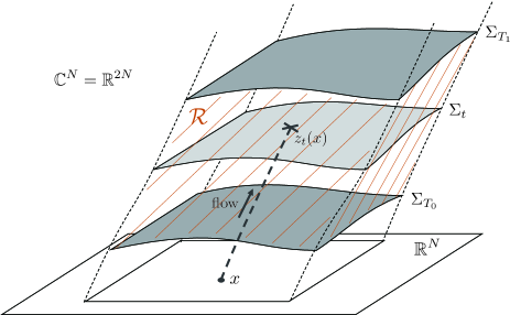
Figure 1: The worldvolume ${\mathcal{R}}$ (shaded region) embedded in ${\mathbb{C}}^{N}={\mathbb{R}}^{2N}$.

Although the weight function $e^{-{W}(t)}$ can be chosen arbitrarily, a practically good choice is the one which gives an almost uniform distribution with respect to $t$ (see subsection 3.4 for details).

The expectation value is now expressed as a ratio of reweighted averages over ${\mathcal{R}}$:

$$\langle\mathcal{O}(x)\rangle=\frac{\int_{\mathcal{R}}{Dz}\,e^{-V(z)}\,{A}(z)\,\mathcal{O}(z)}{\int_{\mathcal{R}}{Dz}\,e^{-V(z)}\,{A}(z)}=\frac{\langle{A}(z)\,\mathcal{O}(z)\rangle_{\mathcal{R}}}{\langle{A}(z)\rangle_{\mathcal{R}}}.$$ (1.15)

Here, the reweighted average

$$\langle f(z)\rangle_{\mathcal{R}}\equiv\frac{\int_{\mathcal{R}}{Dz}\,e^{-V(z)}\,f(z)}{\int_{\mathcal{R}}{Dz}\,e^{-V(z)}}$$ (1.16)

is defined with respect to the (real-valued) invariant volume element ${Dz}$ on the $(N+1)$-dimensional region ${\mathcal{R}}$ and to the new weight

$$e^{-V(z)}\equiv e^{-{\rm Re}\,S(z)-{W}(t(z))}.$$ (1.17)

The accompanying reweighting factor ${A}(z)$ is then given by

$${A}(z)\equiv\frac{e^{-S(z)-{W}(t(z))}dt\,dz_{t}}{e^{-V(z)}{Dz}}=e^{-i\,{\rm Im}\,S(z)}\frac{dt\,dz_{t}}{{Dz}}.$$ (1.18)

The aim of this paper is to establish a HMC algorithm for the reweighted average (1.16) on the worldvolume ${\mathcal{R}}$. To demonstrate that this algorithm works correctly, we apply the algorithm to a chiral random matrix model (the Stephanov model) [28, 29], for which the complex Langevin method is known not to work [30].

This paper is organized as follows. In section 2, we review the basics of the HMC algorithm on a general constrained space ${\mathcal{R}}$. In section 3, we deepen the argument for the case where the constrained surface ${\mathcal{R}}$ is the worldvolume of an integration surface. We first study the geometry of the worldvolume ${\mathcal{R}}$ by using the Arnowitt-Deser-Misner parametrization of the metric. We then construct molecular dynamics on ${\mathcal{R}}$, with a prescription to determine the weight $e^{-{W}(t)}$. After summarizing the HMC algorithm on the worldvolume ${\mathcal{R}}$, we give an algorithm to estimate observables. In section 4, we apply this algorithm to the Stephanov model, and show that our algorithm correctly reproduces exact results, solving both sign and multimodal problems. Section 5 is devoted to conclusion and outlook.

2 HMC algorithm on a constrained space (review)

In this section, we briefly review the basics of the RATTLE algorithm [31, 32], which is a HMC algorithm on a constrained space such as our worldvolume ${\mathcal{R}}$. A detailed discussion is given in appendix A with more geometrical terms.

2.1 Stochastic process on a constrained space

Let ${\mathcal{R}}$ be an $m$-dimensional manifold embedded in the flat space ${\mathbb{R}}^{M}=\{z=(z^{I})\}$ $(I=1,\ldots,M)$. We assume that ${\mathcal{R}}$ is characterized by $M-m$ independent constraint equations $\phi^{r}(z)=0$ $(r=1,\ldots,M-m)$. When ${\mathcal{R}}$ is the worldvolume of an integration surface, we set $M=2N$ and $m=N+1$, treating ${\mathbb{C}}^{N}$ as a real space ${\mathbb{R}}^{2N}$.

Denoting the coordinates on ${\mathcal{R}}$ by $\xi=(\xi^{\mu})$ $(\mu=1,\ldots,m)$, the embedding is expressed by functions $z^{I}=z^{I}(\xi)$, and the induced metric on ${\mathcal{R}}$ is given by

$$ds^{2} =(dz^{I}(\xi))^{2}\equiv g_{\mu\nu}(\xi)\,d\xi^{\mu}d\xi^{\nu}~{}~{}\mbox{with}~{}~{}g_{\mu\nu}(\xi)=\partial_{\mu}z^{I}(\xi)\,\partial_{\nu}z^{I}(\xi),$$ (2.1)

which defines the invariant volume element as

$${Dz}\equiv\sqrt{g(\xi)}\,d\xi,$$ (2.2)

where $d\xi=d\xi^{1}\cdots\xi^{m}$.

The probability distribution $p(z)$ on ${\mathcal{R}}$ is defined with respect to ${Dz}$, and thus is normalized as $\int_{\mathcal{R}}{Dz}\,p(z)=1$. The transition matrix is also defined for ${Dz}$, so that a transition from a probability distribution $p(z)$ to $p^{\prime}(z)$ ($z\in{\mathcal{R}}$) is expressed with a transition matrix $P(z^{\prime}|z)$ as

$$p^{\prime}(z^{\prime})=\int_{\mathcal{R}}{Dz}\,P(z^{\prime}|z)\,p(z)\quad(z^{\prime}\in{\mathcal{R}}).$$ (2.3)

For the equilibrium distribution on ${\mathcal{R}}$ with respect to a potential $V(z)$,

$$p_{\rm eq}(z)\equiv e^{-V(z)}/Z_{\mathcal{R}}\quad\Bigl{(}Z_{\mathcal{R}}=\int_{\mathcal{R}}{Dz}\,e^{-V(z)}\Bigr{)},$$ (2.4)

the detailed balance condition is given by

$$P(z^{\prime}|z)\,e^{-V(z)}=P(z|z^{\prime})\,e^{-V(z^{\prime})}\quad(z,z^{\prime}\in{\mathcal{R}}).$$ (2.5)

Throughout this paper, we denote a function on ${\mathcal{R}}$ by $f(z)$ and $f(\xi)$, interchangeably, with the understanding that $z=z(\xi)$. The transition matrix on ${\mathcal{R}}$ is also written as $P(z^{\prime}|z)$ and $P(\xi^{\prime}|\xi)$ for $z=z(\xi),\,z^{\prime}=z(\xi^{\prime})\in{\mathcal{R}}$.

2.2 HMC on a constrained space

Denoting by $\pi=(\pi^{I})$ the conjugate momentum to $z=(z^{I})\in{\mathcal{R}}$, we consider the Hamiltonian dynamics on ${\mathcal{R}}$ with the Hamiltonian

$$H(z,\pi)=\frac{1}{2}\,(\pi^{I})^{2}+V(z),$$ (2.6)

which can be expressed as a set of first-order differential equations in time $s$ with Lagrange multipliers $\lambda_{r}$:

$$\partial_{s}z =\pi,$$ (2.7)

$$\partial_{s}\pi =-\partial V(z)-\lambda_{r}\,\partial\phi^{r}(z),$$ (2.8)

$$\phi^{r}(z) =0,$$ (2.9)

$$\pi\cdot\partial\phi^{r}(z) =0.$$ (2.10)

Here, $\partial\equiv(\partial_{z^{I}})$ is the gradient in ${\mathbb{R}}^{M}$.

Equations (2.7)–(2.10) can be discretized such that the symplecticity and the reversibility still hold after the discretization (below $\Delta s$ is the step size) [31, 32]:

$$\pi_{1/2} =\pi-\frac{\Delta s}{2}\,\partial V(z)-\lambda_{r}\,\partial\phi^{r}(z),$$ (2.11)

$$z^{\prime} =z+\Delta s\,\pi_{1/2},$$ (2.12)

$$\pi^{\prime} =\pi-\frac{\Delta s}{2}\,\partial V(z^{\prime})-{\lambda^{\prime}}_{r}\,\partial\phi^{r}(z^{\prime}),$$ (2.13)

where $\lambda_{r}$ and $\lambda^{\prime}_{r}$ are determined, respectively, so that the following constraints are satisfied:

$$z^{\prime} \in{\mathcal{R}}\quad(\mbox{i.e.~{}}\phi^{r}(z^{\prime})=0),$$ (2.14)

$$\pi^{\prime} \in T_{z^{\prime}}{\mathcal{R}}.$$ (2.15)

One can easily show that the map $\Phi_{\Delta s}:\,(z,\pi)\rightarrow(z^{\prime},\pi^{\prime})$ actually satisfies the symplecticity and the reversibility (with $\lambda_{r}$ and $\lambda_{r}^{\prime}$ interchanged):

$$\bullet~{}\omega(z^{\prime},\pi^{\prime})=\omega(z,\pi),$$ (2.16)

$$\bullet~{}(z^{\prime},\pi^{\prime})=\Phi_{\Delta s}(z,\pi)\Rightarrow(z,-\pi)=\Phi_{\Delta s}(z^{\prime},-\pi^{\prime}).$$ (2.17)

The Hamiltonian is conserved to the order of $\Delta s^{2}$, i.e., $H(z^{\prime},\pi^{\prime})-H(z,\pi)=O(\Delta s^{3})$.

The HMC algorithm on ${\mathcal{R}}$ then consists of the following three steps for a given initial configuration $z\in{\mathcal{R}}$:

Step 1.

Generate a vector $\tilde{\pi}=(\tilde{\pi}^{I})\in T_{z}{\mathbb{R}}^{M}$ from the Gaussian distribution

$$\frac{1}{(2\pi)^{M/2}}e^{-\tilde{\pi}^{2}/2},$$ (2.18)

and project it onto $T_{z}{\mathcal{R}}$ to obtain an initial momentum $\pi=(\pi^{I})\in T_{z}{\mathcal{R}}$.

Step 2.

Calculate $\Phi_{\Delta s}(z,\pi)$ from (2.11)–(2.15). We repeat this step $n$ times to obtain $(z^{\prime},\pi^{\prime})=\Phi_{\Delta s}^{n}(z,\pi)$.

Step 3.

Update the configuration $z$ to $z^{\prime}$ with a probability

$$\min\big{(}1,e^{-H(z^{\prime},\pi^{\prime})+H(z,\pi)}\big{)}.$$ (2.19)

The above process defines a stochastic process on ${\mathcal{R}}$. One can show that its transition matrix $P(z^{\prime}|z)$ satisfies the detailed balance condition (see appendix A):

$$P(z^{\prime}|z)\,e^{-V(z)}=P(z|z^{\prime})\,e^{-V(z^{\prime})},$$ (2.20)

3 HMC on the worldvolume

In this section, we apply the general formalism in the previous section to the case where ${\mathcal{R}}$ is the worldvolume of an integration surface. We first clarify the geometry of the worldvolume ${\mathcal{R}}$ and then construct the HMC algorithm on ${\mathcal{R}}$.

3.1 Geometry of the worldvolume ${\mathcal{R}}$

Recall that our worldvolume ${\mathcal{R}}$ is an $N+1$-dimensional submanifold embedded in ${\mathbb{C}}^{N}={\mathbb{R}}^{2N}$. As in the previous section, we again assume that ${\mathcal{R}}\subset{\mathbb{R}}^{2N}$ is characterized by a set of independent constraint equations: $\phi^{r}(z)=0$ $(r=1,\cdots,N-1)$. We will often write a point $z=(z^{i})\in{\mathbb{C}}^{N}$ $(i=1,\ldots,N)$ with real coordinates as

$$z=(z^{I})=\left(\begin{array}[]{c}{\rm Re}\,z^{i}\\ {\rm Im}\,z^{i}\end{array}\right)\in{\mathbb{R}}^{2N}\quad(I=1,\ldots,2N).$$ (3.3)

Since $\xi=(\xi^{\mu})\equiv(t,x^{a})$ specifies a point $z(\xi)=(z^{I}(\xi))\equiv(z_{t}^{I}(x))$ in ${\mathcal{R}}$, we can use $\xi$ as coordinates of ${\mathcal{R}}$. The flow equation (1.6) then takes the form

$$\frac{\partial z^{I}}{\partial t}=\partial_{z^{I}}{\rm Re}\,S(z),\quad(z^{I})|_{t=0}=\left(\begin{array}[]{c}x^{i}\\ 0\end{array}\right).$$ (3.6)

Similarly, we write an $N$-dimensional complex vector $v=(v^{i})\in{\mathbb{C}}^{N}$ $(i=1,\ldots,N)$ as a real vector

$$v=(v^{I})=\left(\begin{array}[]{c}{\rm Re}\,v^{i}\\ {\rm Im}\,v^{i}\\ \end{array}\right)\in{\mathbb{R}}^{2N}\quad(I=1,\ldots,2N).$$ (3.9)

The vectors $E_{\mu}=(E^{I}_{\mu}=\partial z^{I}/\partial\xi^{\mu})$ form a basis of $T_{z}{\mathcal{R}}$ (see Fig. 2), from which the induced metric $g_{\mu\nu}$ on ${\mathcal{R}}$ is given by

$$g_{\mu\nu}=E_{\mu}\cdot E_{\nu}.$$ (3.10)

Figure 2: A basis of $T_{z}{\mathcal{R}}$, $\{E_{\mu}\}=\{E_{0},E_{a}\}$. ${\mathcal{R}}$ is drawn one dimension less than in Fig. 1.

Since our worldvolume ${\mathcal{R}}=\bigcup_{t}\Sigma_{t}$ is foliated by the antiholomorphic gradient flow, its intrinsic geometry should be best described (at least for physicists) by the Arnowitt-Deser-Misner (ADM) parametrization, for which the metric is expressed in the form

$$ds^{2}=g_{\mu\nu}(\xi)\,d\xi^{\mu}d\xi^{\nu}=\alpha^{2}(\xi)\,dt^{2}+\gamma_{ab}(\xi)\,(dx^{a}+{\beta}^{a}(\xi)dt)(dx^{b}+{\beta}^{b}(\xi)dt).$$ (3.11)

Here, $\gamma_{ab}$ is the induced metric on $\Sigma_{t}$ (with its inverse matrix $\gamma^{ab}$), ${\beta}^{a}$ is the shift vector, and $\alpha$ is the lapse function,

$$\gamma_{ab} \equiv E_{a}\cdot E_{b},$$ (3.12)

$${\beta}^{a} \equiv\gamma^{ab}\,{\beta}_{b}\equiv\gamma^{ab}\,E_{0}\cdot E_{b},$$ (3.13)

$$\alpha^{2} \equiv E_{0}\cdot E_{0}-\gamma^{ab}\,{\beta}_{a}{\beta}_{b}=E_{0}\cdot(1-\gamma^{ab}\,E_{a}E_{b}^{T})\,E_{0}.$$ (3.14)

The inverse matrix of $(g_{\mu\nu})$ can be easily calculated to be

$$(g^{\mu\nu})=\left(\begin{array}[]{cc}1/{\alpha}^{2}&-{\beta}^{b}/{\alpha}^{2}\\ -{\beta}^{a}/{\alpha}^{2}&{\beta}^{a}{\beta}^{b}/{\alpha}^{2}+\gamma^{ab}\\ \end{array}\right).$$ (3.17)

The geometrical meaning of the ADM parametrization is explained in Fig. 3.

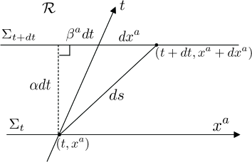
Figure 3: Geometrical meaning of the ADM parametrization. $\alpha\,dt$ is the geodesic distance from a point $\xi=(t,x^{a})$ on $\Sigma_{t}$ to the surface $\Sigma_{t+dt}$. $\beta^{a}dt$ shows that the time axis $t$ is tilted with respect to the normal of $\Sigma_{t}$ by this amount in $x$-coordinates. $\gamma_{ab}$ is the induced metric on $\Sigma_{t}$. The geodesic distance $ds$ between two points $\xi=(t,x^{a})$ and $\xi+d\xi=(t+dt,x^{a}+dx^{a})$ is then obtained from Pythagorean theorem as in (3.11).

Since the flowed surfaces $\Sigma_{t}$ are determined by the flow equation, we can write down the explicit form of the basis $E_{\mu}=(E^{I}_{\mu}=\partial z^{I}/\partial\xi^{\mu})$ of $T_{z}{\mathcal{R}}$ as

$$E^{I}_{0}=\partial_{z^{I}}{\rm Re}\,S(z),\quad E^{I}_{a}=\left(\begin{array}[]{c}{\rm Re}\,J^{i}_{~{}a}\\ {\rm Im}\,J^{i}_{~{}a}\end{array}\right),$$ (3.20)

where we have defined $J(\xi)=J(t,x)\equiv J_{t}(x)$. Thus, the induced metric $\gamma_{ab}$ can be directly expressed in terms of the Jacobian as

$$\gamma_{ab}={\rm Re}\,(J^{\dagger}J)_{ab}=(J^{\dagger}J)_{ab}.$$ (3.21)

The lapse function $\alpha$ can be expressed as the length of the normal component of $E_{0}$:

$${\alpha}^{2}=E_{0}^{\perp}\cdot E_{0}^{\perp}=(E_{0}^{\perp})^{2}.$$ (3.22)

Here, the decomposition of $E_{0}$ to the tangential and normal components is given by

$$E_{0}=E_{0}^{\parallel}+E_{0}^{\perp},$$ (3.23)

$$E_{0}^{\parallel}\equiv\Pi_{\Sigma_{t}}\,E_{0},\quad E_{0}^{\perp}\equiv(1-\Pi_{\Sigma_{t}})\,E_{0},$$ (3.24)

where $\Pi_{\Sigma_{t}}$ is the projector onto $T_{z}\Sigma_{t}$:

$$\Pi_{\Sigma_{t}} \equiv\gamma^{ab}E_{a}E_{b}^{T}.$$ (3.25)

Note that the following relation holds:

$${\beta}^{a}E_{a}=E^{\perp}_{0}.$$ (3.26)

Then, by using (3.17), (3.22), (3.25) and (3.26), we see that the projector from $T_{z}{\mathbb{R}}^{2N}$ onto $T_{z}{\mathcal{R}}$ is given by

$$\Pi_{{\mathcal{R}}} \equiv g^{\mu\nu}E_{\mu}E_{\nu}^{T}=\frac{1}{(E_{0}^{\perp})^{2}}E_{0}^{\perp}(E_{0}^{\perp})^{T}+\Pi_{\Sigma_{t}}.$$ (3.27)

In the ADM parametrization, the volume element of ${\mathcal{R}}$ is given by (see Fig. 4)

$${Dz}=\sqrt{g}\,d\xi=\alpha\,|\det J|\,dt\,dx.$$ (3.28)

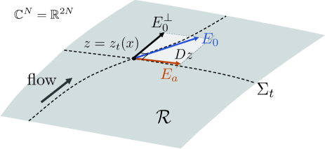
Figure 4: $E_{0}^{\perp}$ and the volume element.

Since the complex measure on $\Sigma_{t}$ is given by $dz_{t}=\det J\,dx$, we find that the reweighting factor (1.18) takes the form

$${A}(z)=\frac{dt\,dz_{t}}{{Dz}}\,e^{-i\,{\rm Im}\,S(z)}=\alpha^{-1}(z)\,e^{i\varphi(z)-i\,{\rm Im}\,S(z)}\quad\Bigl{(}e^{i\varphi(z)}\equiv\frac{\det J}{|\det J|}\Bigr{)}.$$ (3.29)

Note that the inverse lapse, $\alpha^{-1}(z)$, plays the role of the radius of ${A}(z)$.

In appendix B, in order to show the typical behaviors of various geometrical quantities near critical points at large flow times, we give explicit expressions of these quantities for the Gaussian case with the action

$$S(x)=\frac{\beta}{2}\sum_{k=1}^{N}(x^{k}-i)^{2}.$$ (3.30)

There, we find that $\alpha^{-1}(z)$ increases exponentially in flow time $t$ as $z^{k}=z^{k}(t,x)$ approaches the Lefschetz thimble at ${\rm Im}\,z^{k}=1$.

3.2 Molecular dynamics on the worldvolume

We first rewrite the Lagrange multiplier term $\lambda_{r}\,\partial\phi^{r}$ in (2.8) in a more convenient form. Note that $\lambda_{r}\,\partial\phi^{r}$ is normal to ${\mathcal{R}}$, and thus it satisfies

$$(\lambda_{r}\,\partial\phi^{r})\cdot E_{0}=0,\quad(\lambda_{r}\,\partial\phi^{r})\cdot E_{a}=0.$$ (3.31)

Since the vectors

$$F_{a}\equiv\,\left(\begin{array}[]{c}{\rm Im}{J^{i}}_{a}\\ -{\rm Re}\,{J^{i}}_{a}\end{array}\right)\quad(a=1,\ldots,N)$$ (3.34)

span the normal vector space $N_{z}\Sigma_{t}$ at $z\in\Sigma_{t}$, the second equation in (3.31) means that $\lambda_{r}\,\partial\phi^{r}$ can be written as a linear combination of $F_{a}$ with new Lagrange multipliers $\lambda^{a}\in{\mathbb{R}}$ $(a=1,\ldots,N)$:

$$\sum_{r=1}^{N-1}\,\lambda_{r}\,\partial\phi^{r}=\sum_{a=1}^{N}\,\lambda^{a}F_{a}.$$ (3.35)

The first equation in (3.31) is then treated as a constraint on $\lambda^{a}F_{a}$:

$$\lambda^{a}F_{a}\cdot E_{0}=0.$$ (3.36)

From the above argument, we find that the RATTLE algorithm (2.11)–(2.15) can be written as

$$\pi_{1/2} =\pi-\frac{\Delta s}{2}\,\partial V(z)-\lambda^{a}F_{a}(z),$$ (3.37)

$$z^{\prime} =z+\Delta s\,\pi_{1/2},$$ (3.38)

$$\pi^{\prime} =\pi-\frac{\Delta s}{2}\,\partial V(z^{\prime})-{\lambda^{\prime}}^{a}F_{a}(z^{\prime}),$$ (3.39)

where $\lambda^{a}$ and ${\lambda^{\prime}}^{a}$ are determined, respectively, so that the following constraints are satisfied:

$$z^{\prime}\in{\mathcal{R}}\quad \mbox{and}\quad\lambda^{a}F_{a}(z)\cdot E_{0}(z)=0,$$ (3.40)

$$\pi^{\prime}\in T_{z^{\prime}}{\mathcal{R}}\quad \mbox{and}\quad{\lambda^{\prime}}^{a}F_{a}(z^{\prime})\cdot E_{0}(z^{\prime})=0.$$ (3.41)

The gradient of the potential, $\partial V(z)$, now takes the form

$$\partial V(z)=\partial{\rm Re}\,S(z)+{W}^{\prime}(t(z))\,\partial t(z).$$ (3.42)

In order to define the gradient $\partial t(z)$ at $z\in{\mathcal{R}}$, we regard $(\phi^{r})$ as coordinates in the extra dimensions and construct $2N$ coordinates $(\xi^{\mu},\phi^{r})$ in the vicinity of ${\mathcal{R}}$ in ${\mathbb{R}}^{2N}$. Then, one can show (see appendix C) that the gradient $\partial t(z)$ is given by

$$\partial t(z)=\frac{1}{(E_{0}^{\perp})^{2}}\,E_{0}^{\perp}-\frac{E_{r}\cdot E_{0}^{\perp}}{(E_{0}^{\perp})^{2}}\,\partial\phi^{r}(z)\quad(z\in{\mathcal{R}}).$$ (3.43)

Since the last term is a linear combination of the gradients $\partial\phi^{r}(z)$ and thus can be absorbed into the Lagrange multiplier terms in (3.37) and (3.39), we can (and will) set $\partial t(z)$ to the form

$$\partial t(z)=\frac{1}{(E_{0}^{\perp})^{2}}\,E_{0}^{\perp}\quad(z\in{\mathcal{R}}).$$ (3.44)

3.3 Solving the constraints in molecular dynamics

In this subsection, we present numerical algorithms to solve the constraints (3.40) and (3.41).

Solving (3.40)

The condition $z^{\prime}\in{\mathcal{R}}$ for a given $z=z(\xi)\in{\mathcal{R}}$ is equivalent to the existence of an $N+1$-dimensional vector $\varepsilon=(\varepsilon^{\mu})=(h,u^{a})$ such that $z^{\prime}=z(\xi+\varepsilon)=z_{t+h}(x+u)$. Thus, (3.40) can be solved by finding a solution to $2N+1$ equations

$$f^{P}(w)=0\quad(P=0,1,\ldots,2N)$$ (3.45)

for $2N+1$ unknowns $w=(w^{P})=(\varepsilon^{\mu},\lambda^{a})\in{\mathbb{R}}^{2N+1}$ (see Fig. 5), where

$$f^{0}(w) \equiv\lambda^{a}\,F_{a}(\xi)\cdot E_{0}(\xi)=-\lambda^{a}\,{\rm Im}\bigl{[}\partial_{z^{i}}S(z(\xi))\,{J^{i}}_{a}(\xi)\bigr{]},$$ (3.46)

$$f^{I}(w) \equiv z^{I}(\xi+\varepsilon)-z^{I}(\xi)-\Delta z^{I}+\lambda^{a}F_{a}^{I}(\xi)\quad(I=1,\ldots,2N)$$ (3.47)

with

$$\Delta z\equiv\Delta s\,\pi-\frac{\Delta s^{2}}{2}\,\partial V(z).$$ (3.48)

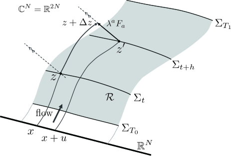
Figure 5: Finding $z^{\prime}=z(\xi+\varepsilon)=z_{t+h}(x+u)$ on ${\mathcal{R}}$ from $z=z(\xi)=z_{t}(x)\in{\mathcal{R}}$.

Adopting Newton’s method to find a solution, we iteratively update the vector $w=(w^{P})=(\varepsilon^{\mu},\lambda^{a})$ as $w\to w+\Delta w$, where $\Delta w$ is a solution of the linear equation

$$\frac{\partial f^{P}(w)}{\partial w^{Q}}\Delta w^{Q}=-f^{P}(w).$$ (3.49)

The matrix elements $\partial f^{P}/\partial w^{Q}$ are easily found to be

$$\Big{(}\frac{\partial f^{P}(w)}{\partial w^{Q}}\Big{)} =\left[\begin{array}[]{ccc}0&0&F_{a}(\xi)\cdot E_{0}(\xi)\\ E^{I}_{0}(\xi+\varepsilon)&E^{I}_{a}(\xi+\varepsilon)&F^{I}_{a}(\xi)\\ \end{array}\right]$$ (3.52)

$$=\left[\begin{array}[]{ccc}0&0&-{\rm Im}\,\bigl{[}\partial_{z^{i}}S(z(\xi))\,{J^{i}}_{a}(\xi)\bigr{]}\\ {\rm Re}\,\bigl{[}\partial_{z^{i}}S(z(\xi+\varepsilon))\bigr{]}&{\rm Re}\,{J^{i}}_{a}(\xi+\varepsilon)&-{\rm Im}\,{J^{i}}_{a}(\xi)\\ -{\rm Im}\,\bigl{[}\partial_{z^{i}}S(z(\xi+\varepsilon))\bigr{]}&{\rm Im}\,{J^{i}}_{a}(\xi+\varepsilon)&{\rm Re}\,{J^{i}}_{a}(\xi)\\ \end{array}\right].$$ (3.56)

When the DOF $(=N)$ is small, (3.49) can be solved by a direct method such as the LU decomposition of (3.56), for which we integrate the second flow equation (1.12) to know the value of $J$. When the DOF is large, the computation of $J$ becomes expensive, and we can instead use an iterative method such as GMRES [33] or BiCGStab [34], for which we do not need to compute the matrix elements of $J$ as in [18]. To see this, we first note that the right hand side of (3.49) can be written in terms of complex vectors as

$$f^{0}(w) =-{\rm Im}\,\bigl{[}\partial_{z^{i}}S(z(\xi))\,{J^{i}}_{a}(\xi)\lambda^{a}\bigr{]},$$ (3.57)

$$f^{i}(w) =z^{i}(\xi+\varepsilon)-z^{i}(\xi)-\Delta z^{i}+i{J^{i}}_{a}(\xi)\lambda^{a}.$$ (3.58)

The left hand side of (3.49) can also be written as

$$\frac{\partial f^{0}(w)}{\partial w^{N}}\,\Delta w^{N} =-{\rm Im}\,\bigl{[}\partial_{z^{i}}S(z(\xi))\,{J^{i}}_{a}(\xi)\Delta\lambda^{a}\bigr{]},$$ (3.59)

$$\frac{\partial f^{i}(w)}{\partial w^{N}}\,\Delta w^{N} =[\partial_{z^{i}}S(z(\xi+\varepsilon))]^{\ast}+{J^{i}}_{a}(\xi+\varepsilon)\Delta u^{a}+i{J^{i}}_{a}(\xi)\Delta\lambda^{a}.$$ (3.60)

We thus see that in the above equations, $J$ appears only in the form ${J^{i}}_{a}(\xi)v^{a}$ or ${J^{i}}_{a}(\xi+\varepsilon)v^{a}$ with a real vector $v=(v^{a})\in{\mathbb{R}}^{N}$. The former can be evaluated from the solution to the flow equation (1.6) and the following equation [see (1.12)]:

$$\dot{v}_{t}^{i}=[H_{ij}(z_{t})\,v_{t}^{j}]^{\ast},\quad v^{i}_{t=0}=v^{i},$$ (3.61)

by setting ${J^{i}}_{a}(\xi)v^{a}=v_{t}^{i}$. The latter is obtained in a similar way, by replacing $t\to t+h$ and $x^{a}\to x^{a}+u^{a}$. We thus find that the both hand sides of (3.49) can be calculated without computing the matrix elements of $J$.

Solving (3.41)

We first note that solving the constraint (3.41) is equivalent to projecting the vector

$$\tilde{\pi}^{\prime} \equiv\pi-\frac{\Delta s}{2}\,\partial V(z^{\prime})$$ (3.62)

onto $T_{z^{\prime}}{\mathcal{R}}$ [see (3.27)]:

$$\pi^{\prime} \equiv\Pi_{{\mathcal{R}}}(z^{\prime})\,\tilde{\pi}^{\prime}=\frac{E_{0}^{\perp}(z^{\prime})\cdot\tilde{\pi}^{\prime}}{(E_{0}^{\perp}(z^{\prime}))^{2}}\,E_{0}^{\perp}(z^{\prime})+\Pi_{\Sigma_{t}}(z^{\prime})\,\tilde{\pi}^{\prime}.$$ (3.63)

Here, $E_{0}^{\perp}(z^{\prime})$ can be computed as a complex vector to be

$$E_{0}^{\perp}(z^{\prime})=iJ(z^{\prime})\,{\rm Im}\,\bigl{(}J^{-1}(z^{\prime})\,[\partial S(z^{\prime})]^{\ast}\bigr{)}.$$ (3.64)

The second term in (3.63) can also be computed as

$$\Pi_{\Sigma_{t}}(z^{\prime})\,\tilde{\pi}^{\prime}=J(z^{\prime})\,{\rm Re}\,\bigl{(}J^{-1}(z^{\prime})\,\tilde{\pi}^{\prime}\bigr{)}.$$ (3.65)

The expressions (3.64) and (3.65) can again be evaluated either by a direct method with the computation of $J(z^{\prime})$, or by an iterative method without computing $J(z^{\prime})$ as in [18]. When the iterative method is used, the inversion $J^{-1}(z^{\prime})\,c$ is obtained for a given complex vector $c=(c^{i})\in{\mathbb{C}}^{N}$ by looking for vectors $a=(a^{a}),\,b=(b^{a})\in{\mathbb{R}}^{N}$ iteratively such that

$$c=J(z^{\prime})\,a+iJ(z^{\prime})\,b,$$ (3.66)

where $J(z^{\prime})\,a$ and $J(z^{\prime})\,b$ are evaluated by integrating the flow equation (3.61) with the initial condition $v_{t=0}=a$ and $v_{t=0}=b$, respectively. The multiplication $J(z^{\prime})\,v$ are again calculated by integrating (3.61). Therefore, the projection (3.63) can be performed without computing $J(z^{\prime})$.

Note that every time we evaluate $\partial V(z)$ [eq. (3.42)], we need $\partial t(z)$ and thus $E_{0}^{\perp}(z)$ [see (3.44)]. $E_{0}^{\perp}(z)$ can be calculated from (3.64) by replacing $z^{\prime}$ with $z$.

3.4 Construction of ${W}(t)$

In this subsection, we present a prescription to construct a weight function $e^{-{W}(t)}$ in (1.13) [or in (1.17)] so that it gives an almost uniform distribution with respect to $t$. The key is that, for a given weight $e^{-{W}(t)}$, the probability to find a configuration at $t$ is proportional to

$$Z(t;{W})\equiv e^{-{W}(t)}\int_{{\mathbb{R}}^{N}}dx\,{\alpha}(t,x)|\det J(t,x)|e^{-{\rm Re}\,S(z(t,x))}.$$ (3.67)

Thus, when a weight $e^{-{W}(t)}$ does not give a uniform distribution of $t$, the desired weight can be obtained by (see e.g., [35])

$${W}^{\rm(new)}(t)={W}(t)+\ln Z(t;{W})+\mbox{const},$$ (3.68)

because then $Z(t;{W}^{\rm(new)})$ becomes constant in $t$:

$$Z(t;{W}^{\rm(new)}) =e^{-{W}^{\rm(new)}(t)}\int_{{\mathbb{R}}^{N}}dx\,{\alpha}(t,x)\,|\det J(t,x)|\,e^{-{\rm Re}\,S(z(t,x))}$$

$$={\rm const}\,\frac{e^{-{W}(t)}}{Z(t;{W})}\cdot e^{{W}(t)}\,Z(t;{W})=\mbox{const}.$$ (3.69)

Of course, the above procedure is possible only when we know the values of $Z(t;{W})$ explicitly, which is usually not the case. However, we can estimate $Z(t;{W})$ from the histogram of flow times $\{t\}$. To be more specific, we first divide the interval $[T_{0},T_{1}]$ into $p+1$ bins, $I_{\ell}\equiv[\ell h,(\ell+1)h]$ $(\ell=0,\ldots,p)$ with $h\equiv(T_{1}-T_{0})/(p+1)$, and generate a certain number ($\equiv n_{\rm tune}$) of configurations by using $V(z)={\rm Re}\,S(z)+{W}(t(z))$ as the potential. The numbers $h_{\ell}$ of configurations inside the bins $I_{\ell}$ give a rough estimate of the functional form of $Z(t;{W})$ up to a normalization factor (see Fig. 6).

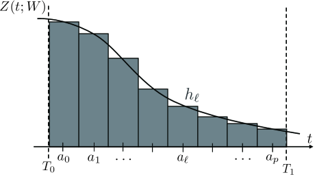
Figure 6: Estimating $Z(t;{W})$ from $\{h_{\ell}\}$.

Then, from the histogram $h_{\ell}$ $(\ell=0,\ldots,p)$, we calculate

$${W}^{\rm(new)}_{\ell}={W}(a_{\ell})+\ln h_{\ell},$$ (3.70)

and construct a function $W^{\rm(new)}(t)$ to be approximated by a polynomial satisfying $W^{\rm(new)}(a_{\ell})=W^{\rm(new)}_{\ell}$ with $a_{\ell}\equiv(\ell+1/2)h$.

In general, the minimum-order polynomial that have values $b_{\ell}$ at $a_{\ell}=(\ell+1/2)h$ is given by the Lagrange interpolation of the form

$$L(t;\{b_{\ell}\})\equiv\sum_{\ell=0}^{p}\frac{\prod_{m\neq\ell}(t-a_{m})}{\prod_{m\neq\ell}(a_{\ell}-a_{m})}\,b_{\ell}=\sum_{\ell=0}^{p}\Bigl{[}\prod_{m<\ell}(t-a_{\ell})\Bigr{]}\,\frac{\Delta^{\ell}b_{0}}{\ell!\,h^{\ell}},$$ (3.71)

where, for an array $\{v_{0},v_{1},v_{2},\ldots\}$, we define $\Delta v_{\ell}\equiv v_{\ell+1}-v_{\ell}$, so that

$$\Delta^{\ell}v_{0}=\sum_{k=0}^{\ell}(-1)^{k}\binom{\ell}{k}\,v_{\ell-k}.$$ (3.72)

Using this polynomial, we define

$${W}^{\rm(new)}(t)\equiv L(t;\{{W}^{\rm(new)}_{\ell}\}).$$ (3.73)

Since the estimate of $Z(t;{W})$ from the histogram $\{h_{\ell}\}$ includes statistical errors, we use an iterative algorithm to update $\{{W}_{\ell}\}$ until an almost uniform distribution is obtained:

• Initialize $\{{W}_{\ell}\}$ with appropriate values (e.g., ${W}_{\ell}^{(0)}=0$).

• From an array $\{{W}^{(k)}_{\ell}\}$, construct an order-$(p+1)$ polynomial $L(t;\{W^{(k)}_{\ell}\})$, and set $W^{(k)}(t)\equiv L(t;\{W^{(k)}_{\ell}\})$.

• Generate $n_{\rm tune}$ configurations with the potential $V(z)={\rm Re}\,S(z)+W^{(k)}(t(z))$, and record the numbers $h_{\ell}^{(k)}$ of configurations in the intervals $I_{\ell}$.

• Update $\{{W}_{\ell}\}$ as ${W}_{\ell}^{(k+1)}\equiv{W}_{\ell}^{(k)}+\ln(h_{\ell}^{(k)}+\epsilon_{c})$. Here, $\epsilon_{c}$ is a cutoff to avoid the divergence arising when $h^{(k)}_{\ell}=0$.

• Terminate the iteration when the histogram becomes almost flat. We use the following stopping condition:

  $$\frac{1}{p}\sum_{l=0}^{p-1}\Big{[}\frac{h_{l+1}-h_{l}}{(h_{l+1}+h_{l})/2}\Big{]}^{2}<\delta^{2}.$$ (3.74)

In the calculation below, we set $p=7$, $n_{\rm tune}=(p+1)\times 200=1,600$, $\epsilon_{c}=0.01$, and $\delta^{2}=0.2$.

3.5 Summary of the HMC algorithm on the worldvolume

We summarize the HMC algorithm for a given initial configuration $z\in{\mathcal{R}}$.

Step 1.

Generate $\tilde{\pi}=(\tilde{\pi}^{I})$ from the Gaussian distribution, and project it onto $T_{z}{\mathcal{R}}$ to obtain an initial momentum $\pi=(\pi^{I})$: $\pi=\Pi_{\mathcal{R}}(z)\,\tilde{\pi}$.

Step 2.

Calculate $(z,\pi)\to\Phi_{\Delta s}(z,\pi)$ with (3.37)–(3.41). The gradient $\partial V(z)$ takes the form (3.42), where $\partial t(z)$ is given by (3.44) and $W(t)$ is determined from test runs by using the iterative algorithm given in subsection 3.4. The first constraint (3.40) is solved by finding a root of the functions (3.46) and (3.47), and the second constraint (3.41) is solved by calculating (3.62) and (3.63). We repeat this process $n$ times to obtain $(z^{\prime},\pi^{\prime})=\Phi^{n}_{\Delta s}(z,\pi)$.

Step 3.

Update the configuration $z$ to $z^{\prime}$ with a probability

$$\min\big{(}1,e^{-H(z^{\prime},\pi^{\prime})+H(z,\pi)}\big{)}.$$ (3.75)

Upon measurement, we further compute the reweighting factor ${A}(z)$ [see (3.29)], which requires the phase $e^{i\varphi(z)}=\det J(z)/|\det J(z)|$, that is evaluated by first solving (1.12) to get $J(z)$ and then computing its determinant. The lapse function ${\alpha}(z)=|E_{0}^{\perp}(z)|$ is already obtained in the preceding molecular dynamics step (Step 2).

In the course of molecular dynamics (Step 2), it sometimes happens that the equation $(z^{\prime},\pi^{\prime})=\Phi_{\Delta s}(z,\pi)$ does not have a solution because $z+\Delta z$ passes over the boundary of ${\mathcal{R}}$ (see Fig. 7).

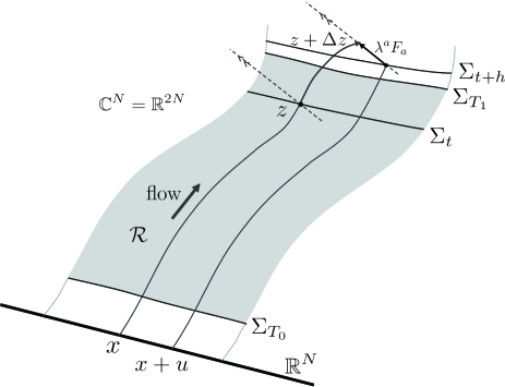
Figure 7: A transition passing over the boundary at $T_{1}$.

Here, the boundary in the $t$ direction is given by $T_{0},\,T_{1}$, while that in the $x$ direction by zeros of $e^{-S(z)}$. When a solution is not found near a boundary, we replace the operator $\Phi_{\Delta s}$ by the momentum reflection $\mathcal{T}$:

$$\mathcal{T}(z,\pi)\equiv(z,\pi^{\prime}),$$ (3.76)

where for $\pi$ which is expanded with $E^{\mu}\equiv g^{\mu\nu}E_{\nu}$ as $\pi=\eta_{0}E^{0}+\eta_{a}E^{a}$, the reflected momentum $\pi^{\prime}$ is defined by $\pi^{\prime}\equiv-\eta_{0}E^{0}+\eta_{a}E^{a}=\pi-2\eta_{0}E^{0}$, i.e.,

$$\pi^{\prime}\equiv\pi-2\,\frac{E_{0}\cdot\pi}{{E_{0}^{\perp}}^{2}}\,E_{0}^{\perp}.$$ (3.77)

This preserves the reversibility and the phase-space volume element because the induced symplectic form is given by $\omega=d\eta_{\mu}\wedge d\xi^{\mu}=d\eta_{0}\wedge d\xi^{0}+d\eta_{a}\wedge d\xi^{a}$ (see appendix A). However, this can change the value of the Hamiltonian. The change comes only from the difference between the norms of momenta $\pi$ and $\pi^{\prime}$, and its effect is absorbed in the probability at the Metropolis test in Step 3 above, so that the detailed balance condition (2.20) still holds. If the change is larger than a prescribed value (e.g., if $e^{-|\Delta H|}=e^{-|{\pi^{\prime}}^{2}-\pi^{2}|/2}<0.8$), we instead use the momentum flip $\Psi$ [20]:

$$\Psi(z,\pi)\equiv(z,-\pi).$$ (3.78)

Since the replacement of $\Phi_{\Delta s}$ by $\mathcal{T}$ or $\Psi$ preserves the phase-space volume element and the reversibility, the detailed balance condition (2.20) still holds.

3.6 Estimation of observables

We first recall that the boundary flow times ($T_{0}$ and $T_{1}$) can be chosen arbitrarily due to Cauchy’s theorem. In practice, $T_{0}$ must be set sufficiently small in order to keep in ${\mathcal{R}}$ a region that is free from multimodality (to be set to $T_{0}=0$ when the multimodal problem is absent there). On the other hand, $T_{1}$ must be taken sufficiently large in order to keep a region where the sign problem is resolved, but, at the same time, $T_{1}$ should not be set too large in order to avoid introducing an unnecessarily large computational time.

When estimating observables, we take a subinterval in $[T_{0},T_{1}]$ (to be denoted by $[\hat{T}_{0},\hat{T}_{1}]$). Namely, for a sample of configurations that are generated in the range $[T_{0},T_{1}]$ (with sample size $N_{\rm conf}$), we construct a subsample $\{z^{(k)}\}$ $(k=1,\dots,\hat{N}_{\rm conf})$ taking configurations from the interval $[\hat{T}_{0},\hat{T}_{1}]$ $(T_{0}\leq\hat{T}_{0}<\hat{T}_{1}\leq T_{1})$, and take a ratio of sample averages over this subsample,

$$\bar{\mathcal{O}}(\hat{T}_{0},\hat{T}_{1})\equiv\frac{(1/\hat{N}_{\rm conf})\,\sum_{k}{A}(z^{(k)})\,\mathcal{O}(z^{(k)})}{(1/\hat{N}_{\rm conf})\,\sum_{k}{A}(z^{(k)})}.$$ (3.79)

$\hat{T}_{0}$ now should be set sufficiently large in order to exclude a region that is contaminated by the sign problem. Note that $\hat{T}_{0}$ and $\hat{T}_{1}$ should be set enough apart in order to maintain a sufficient size for the subsample. Then, if the original range $[T_{0},T_{1}]$ is properly chosen as above, and if the system is well close to global equilibrium, there must be a region in two-parameter space $(\hat{T}_{0},\hat{T}_{1})$ such that the estimations $\bar{\mathcal{O}}(\hat{T}_{0},\hat{T}_{1})$ are stable against the variation of the estimation ranges (i.e., estimates change only within statistical errors).

The whole process of the WV-TLTM thus proceeds as follows:

1. Choose a sufficiently small $T_{0}$ and a sufficiently large $T_{1}$ to tame both sign and multimodal problems.

2. Construct a weight function $e^{-{W}(t)}$ such that the distribution of $t$ becomes almost uniform (see subsection 3.4 for more details).

3. Use the HMC algorithm in subsection 3.5 to generate configurations in the range $[T_{0},T_{1}]$ from the distribution $\propto e^{-V(z)}$ with $V(z)={\rm Re}\,S(z)+{W}(t(z))$.

4. For the obtained full sample, vary the estimation range $[\hat{T}_{0},\hat{T}_{1}]$, looking for a stable region (plateau) in the two-parameter space $(\hat{T}_{0},\hat{T}_{1})$ that give the same estimate $\bar{\mathcal{O}}(\hat{T}_{0},\hat{T}_{1})$ within statistical errors.

5. Choose a point $(\hat{T}_{0},\hat{T}_{1})$ from the plateau and take the corresponding $\bar{\mathcal{O}}(\hat{T}_{0},\hat{T}_{1})$ as the estimate of $\langle\mathcal{O}(x)\rangle$. The error of estimation is read from the statistical error for the chosen subsample.

4 Application to a chiral random matrix model

In this section, to confirm that the WV-TLTM works correctly, we apply the WV-TLTM to a chiral random matrix model, the Stephanov model [28, 29]. We show that the algorithm correctly reproduces exact results, solving both sign and multimodal problems.

4.1 The model

The Stephanov model is a large $N$ matrix model that approximates QCD at finite density. For $N_{f}$ quarks with equal mass $m$, the partition function is given by the following integral over $n\times n$ complex matrices $X=(X_{ij}=x_{ij}+i\,y_{ij})$:

$$Z_{n}^{N_{f}}=e^{n\mu^{2}}\int d^{2}X\,e^{-S(X,X^{\dagger})}\equiv e^{n\mu^{2}}\int d^{2}X\,e^{-n\,{\rm tr}\,X^{\dagger}X}\,{\det}^{N_{f}}(D+m).$$ (4.1)

Here, $D+m$ represents the Dirac operator in the chiral representation and takes the form

$$D+m\equiv\left(\begin{array}[]{cc}m\,1_{n}&i\,(X+C)\\ i\,(X^{\dagger}+C)&m\,1_{n}\end{array}\right),$$ (4.4)

where

$$i\,C\equiv\left(\begin{array}[]{cc}(\mu+i\tau)\,1_{n/2}&0\\ 0&(\mu-i\tau)\,1_{n/2}\end{array}\right).$$ (4.7)

The parameters $\mu$ and $\tau$ correspond to the chemical potential and the temperature, respectively [28, 29]. The number of DOF is $N=2n^{2}$, which may be compared with the DOF of the $SU(N_{c})$ gauge field on the lattice of linear size $L$ as $N=4(N_{c}^{2}-1)L^{4}$.

For the case $N_{f}=1$, the partition function at finite $n$ can be written as an integral over a single variable:

$$Z_{n}^{N_{f}=1}=n\,e^{n(\mu^{2}-m^{2})}\,\int_{0}^{\infty}d\rho\,e^{-n\rho}\,I_{0}(2nm\sqrt{\rho})\,\bigr{[}(\rho-\mu^{2}+\tau^{2})^{2}+(2\mu\tau)^{2}\bigr{]}^{n/2},$$ (4.8)

where $I_{k}(x)$ $(k=0,1,2,\cdots)$ are the modified Bessel functions of the first kind. Then, the chiral condensate is expressed as

$$\langle\bar{\psi}\psi\rangle \equiv\frac{1}{2n}\,\frac{\partial}{\partial m}\,\ln Z_{n}^{N_{f}=1}$$

$$=-m+\frac{\int_{0}^{\infty}d\rho\,e^{-n\rho}\,I_{1}(2nm\sqrt{\rho})\,\sqrt{\rho}\,\bigr{[}(\rho-\mu^{2}+\tau^{2})^{2}+(2\mu\tau)^{2}\bigr{]}^{n/2}}{\int_{0}^{\infty}d\rho\,e^{-n\rho}\,I_{0}(2nm\sqrt{\rho})\,\bigr{[}(\rho-\mu^{2}+\tau^{2})^{2}+(2\mu\tau)^{2}\bigr{]}^{n/2}}.$$ (4.9)

Similarly, the number density is expressed as

$$\langle\psi^{\dagger}\psi\rangle \equiv\frac{1}{2n}\,\frac{\partial}{\partial\mu}\,\ln Z_{n}^{N_{f}=1}$$

$$=\mu-\mu\,\frac{\int_{0}^{\infty}d\rho\,e^{-n\rho}\,I_{0}(2nm\sqrt{\rho})\,\bigr{[}(\rho-\mu^{2}+\tau^{2})^{2}+(2\mu\tau)^{2}\bigr{]}^{n/2-1}\,(\rho-\mu^{2}-\tau^{2})}{\int_{0}^{\infty}d\rho\,e^{-n\rho}\,I_{0}(2nm\sqrt{\rho})\,\bigr{[}(\rho-\mu^{2}+\tau^{2})^{2}+(2\mu\tau)^{2}\bigr{]}^{n/2}}.$$ (4.10)

We apply the WV-TLTM to this model, by complexifying the real and imaginary parts ($x_{ij}$ and $y_{ij}$) separately, and by considering the antiholomorphic gradient flow with respect to the action given in (4.1). We estimate the chiral condensate and the number density using the formulas

$$\langle\bar{\psi}\psi\rangle =\frac{1}{2n}\,\langle{\rm tr}\,(D+m)^{-1}\rangle,\quad$$ (4.11)

$$\langle\psi^{\dagger}\psi\rangle =\mu+\frac{1}{2n}\,\Bigl{\langle}{\rm tr}\,\Bigl{[}(D+m)^{-1}\left(\begin{array}[]{cc}0&1_{n}\\ 1_{n}&0\end{array}\right)\Bigr{]}\Bigr{\rangle}.$$ (4.14)

It is convenient to introduce the matrices

$$A\equiv X+C,\quad B\equiv X^{\dagger}+C,\quad K\equiv(BA+m^{2})^{-1},$$ (4.15)

with which $D+m$ and $(D+m)^{-1}$ are expressed as

$$D+m =\left(\begin{array}[]{cc}m\,1_{n}&i\,A\\ i\,B&m\,1_{n}\end{array}\right),$$ (4.18)

$$(D+m)^{-1} =\left(\begin{array}[]{cc}m\,(AB+m^{2})^{-1}&-i\,A(BA+m^{2})^{-1}\\ -i\,(BA+m^{2})^{-1}B&m\,(BA+m^{2})^{-1}\end{array}\right)$$ (4.21)

$$=\left(\begin{array}[]{cc}m\,AKA^{-1}&-i\,AK\\ -i\,KB&m\,K\end{array}\right).$$ (4.24)

The flow equation is then written only with $A,\,B,\,K$, and the expectation values (4.11) and (4.14) are estimated from the expressions

$$\langle\bar{\psi}\psi\rangle =\frac{m}{n}\,\langle{\rm tr\,}K\rangle,\quad$$ (4.25)

$$\langle\psi^{\dagger}\psi\rangle =\mu-\frac{i}{2n}\,\langle{\rm tr\,}K(A+B)\rangle.$$ (4.26)

4.2 Setup in the simulation

We summarize the setup in the simulation. We set $n=10$, $m=0.004$, $\tau=0$, and estimate the chiral condensate $\langle\bar{\psi}\psi\rangle$ and the number density $\langle\psi^{\dagger}\psi\rangle$ as functions of $\mu=0.4,\ldots,0.8$.

We set $T_{0}=0$ while we choose $T_{1}$ depending on $\mu$ as in Table 1. Other simulation parameters are also given in Table 1.

$\mu$	$0.4$	$0.45$	$0.5$	$0.55$	$0.575$	$0.6$
$T_{0}$	0	0	0	0	0	0
$T_{1}$	0.025	0.048	0.056	0.068	0.068	0.068
$N_{\rm init}$	80	60	40	100	100	50
$N_{\rm conf}$	4,000	4,000	4,000	12,000	10,000	6,000
$\hat{T}_{0}$ ($\langle\bar{\psi}\psi\rangle$)	0.0145	0.02784	0.028	0.04352	0.04216	0.0272
$\hat{T}_{1}$ ($\langle\bar{\psi}\psi\rangle$)	0.025	0.048	0.056	0.068	0.068	0.06664
$N_{\rm conf}(\hat{T}_{0},\hat{T}_{1})$ ($\langle\bar{\psi}\psi\rangle$)	1,600	1,600	1,800	4,400	4,400	3,600
$\hat{T}_{0}$ ($\langle\psi^{\dagger}\psi\rangle$)	0.0095	0.02112	0.03472	0.04624	0.03128	0.04352
$\hat{T}_{1}$ ($\langle\psi^{\dagger}\psi\rangle$)	0.025	0.048	0.056	0.068	0.068	0.068
$N_{\rm conf}(\hat{T}_{0},\hat{T}_{1})$ ($\langle\psi^{\dagger}\psi\rangle$)	2,400	2,400	1,250	3,500	6,000	2,200
$\mu$	$0.625$	$0.65$	$0.7$	$0.75$	$0.8$
$T_{0}$	0	0	0	0	0
$T_{1}$	0.068	0.064	0.06	0.052	0.04
$N_{\rm init}$	40	75	50	40	40
$N_{\rm conf}$	5,000	8,000	4,000	4,000	4,000
$\hat{T}_{0}$ ($\langle\bar{\psi}\psi\rangle$)	0.02312	0.02432	0.0204	0.01456	0.0136
$\hat{T}_{1}$ ($\langle\bar{\psi}\psi\rangle$)	0.068	0.064	0.06	0.052	0.04
$N_{\rm conf}(\hat{T}_{0},\hat{T}_{1})$ ($\langle\bar{\psi}\psi\rangle$)	3,500	5,500	2,600	2,500	2,600
$\hat{T}_{0}$ ($\langle\psi^{\dagger}\psi\rangle$)	0.02448	0.01664	0.0252	0.02496	0.0264
$\hat{T}_{1}$ ($\langle\psi^{\dagger}\psi\rangle$)	0.068	0.064	0.06	0.052	0.04
$N_{\rm conf}(\hat{T}_{0},\hat{T}_{1})$ ($\langle\psi^{\dagger}\psi\rangle$)	3,000	6,500	2,500	1,750	1,200

Table 1: Simulation parameters.

There, $N_{\rm init}$ is the number of initial configurations, and $N_{\rm conf}$ is the number of configurations in the simulation range $[T_{0},T_{1}]$, while $N_{\rm conf}(\hat{T}_{0},\hat{T}_{1})$ is that in the estimation range $[\hat{T}_{0},\hat{T}_{1}]$, corresponding to the point $(\hat{T}_{0},\hat{T}_{1})$ chosen from a plateau. Note that $\hat{T}_{0}$ and $T_{1}$ depend on the choice of observables. We set the initial configuration to the final configuration in the test run determining ${W}(t)$. The tuning of ${W}(t)$ turns out to take two iterations to realize the condition (3.74). In Fig. 8, we show the final form of ${W}(t)$ at $\mu=0.625$ and the resulting histogram of $t$.

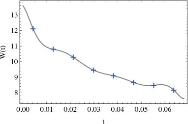
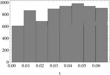
Figure 8: (Left) Final $\{{W}_{\ell}\}$ and its polynomial fit ${W}(t)$. (Right) Final histogram of $t$.

It sometimes happens that ${\mathcal{R}}=\bigcup_{t}\Sigma_{t}$ is not well explored for large $t$ because of the complicated geometrical structure there. To facilitate transitions, at every start of the HMC algorithm we change the step size $\Delta s$ and the step number $n$ by randomly taking them from a set $\mathcal{C}=\{(\Delta_{c},n_{c}\}$ $(c=1,\ldots,c_{\rm max})$. In the calculation below, we set $c_{\rm max}=3$ and choose $\mathcal{C}$ as in Table 2.

index ${c}$	$0$	$1$	$2$	$3$
$\Delta s_{c}$	0.01	0.005	0.001	0.00025
$n_{c}$	25	50	50	100

Table 2: HMC parameters.

We comment that, if we use the original TLTM based on the parallel tempering, we need about 70 replicas for $n=10$. We list in Table 3 the numbers of replicas at $\mu=0.6$ for various $n$.

$n$	4	6	8	10
$T$	0.	0.02	0.06	0.068
#replicas	1	4	$\sim$ 33	$\sim$ 70

Table 3: Maximum flow time $T$ and the number of replicas at $\mu=0.6$.

Here, we first determine the maximum flow time $T$ so that the sign problem is well resolved there, and then determine the number of replicas so that the acceptance rate of the swapping is in the range 0.2–0.5.

4.3 Results and analysis

Figure 9 shows the average reweighting factors from the naive reweighting method (blue) and from the WV-TLTM (orange), the former exhibiting the existence of the sign problem around $\mu=0.6$.

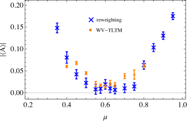
Figure 9: Average phase factors $\langle A\rangle=\langle e^{-i\,{\rm Im}\,S(x)}\rangle_{\rm rewt}$ from the naive reweighting method (blue) and the average reweighting factors $\langle A\rangle=\langle A(z)\rangle_{\mathcal{R}}$ from the WV-TLTM (orange). The estimation range $[\hat{T}_{0},\hat{T}_{1}]$ in the WV-TLTM is set to that for the chiral condensate (see Table 1).

Figure 10 gives the estimates of $\langle\bar{\psi}\psi\rangle$ from the WV-TLTM at $\mu=0.625$ with various estimation ranges $[\hat{T}_{0},\hat{T}_{1}]$.

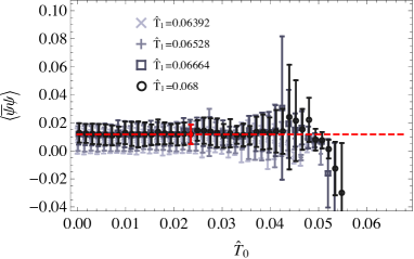
Figure 10: Estimates of $\langle\bar{\psi}\psi\rangle$ at $\mu=0.625$ with various $\hat{T}_{0}$ and $\hat{T}_{1}$. The red filled circle is the point taken from a plateau to be used for the estimation of $\langle\bar{\psi}\psi\rangle$, and the horizontal dashed line is the estimate.

We see a plateau with a value close to the exact one 0.012. Figure 11 exhibits the estimated values thus obtained for the chiral condensate $\langle\bar{\psi}\psi\rangle$ and the number density $\langle\psi^{\dagger}\psi\rangle$.

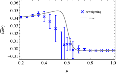
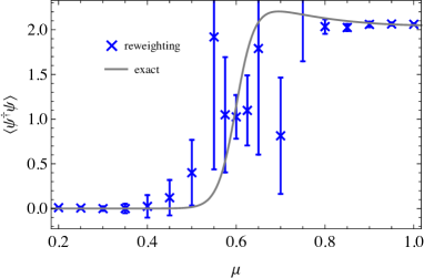
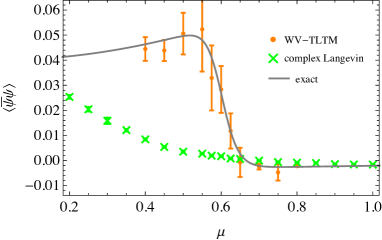
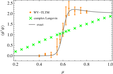
Figure 11: (Left) The chiral condensate. (Right) The Number density. The top panels are the results from the reweighting method, and the bottom panels are from the WV-TLTM and the complex Langevin method.

As a comparison, we also display in the same figure the results from the naive reweighting method and the complex Langevin method, both with the sample size $N_{\rm conf}=10,000$. We see that the WV-TLTM correctly reproduces exact values, while the complex Langevin method suffers from the wrong convergence even for a parameter region free from the sign problem.

One may find it strange that correct estimates are still obtained from the WV-TLTM even for such parameters that give small average reweighting factors $\langle{A}(z)\rangle_{\mathcal{R}}$ (see Fig.9). To understand this, let us see Figs. 12 and 13, which show the histogram of ${A}(z)=\alpha^{-1}(z)\,e^{-i\,{\rm Im}\,S(z)+i\varphi(z)}$, and those of its modulus and phase, in the estimation range $[\hat{T}_{0},\hat{T}_{1}]$ at $\mu=0.625$.

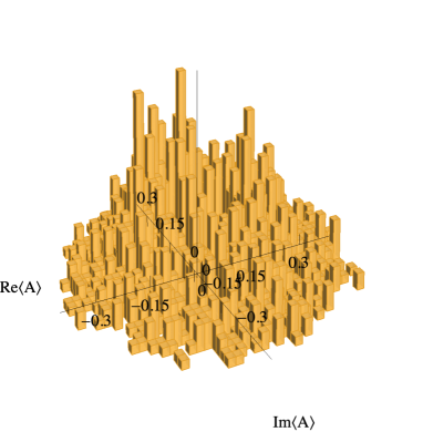
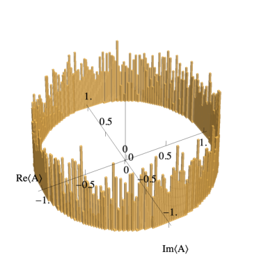
Figure 12: (Left) Histogram of ${A}(z)=\alpha^{-1}(z)\,e^{i\varphi(z)-i{\rm Im}\,S(z)}$ obtained from the WV-TLTM. (Right) Histogram of the phase factor $e^{i\varphi(z)-i{\rm Im}\,S(z)}$ obtained from the reweighting. Both figures are at $\mu=0.625$.

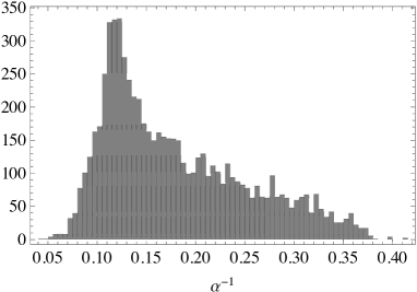
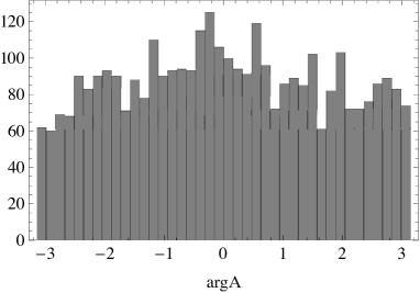
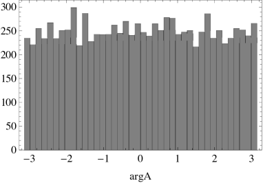
Figure 13: (Top) Histograms of the modulus $|{A}(z)|=\alpha^{-1}(z)$ and the phase ${\rm arg}\,{A}(z)=\varphi(z)-{\rm Im}\,S(z)$ from the WV-TLTM. (Bottom) Histogram of the phase from the reweighting method.

We observe that the distribution of $\alpha^{-1}(z)$ has a peak around $\alpha^{-1}(z)=0.12$. The point is that this small value reduces not only the mean value of ${A}$, but also the statistical errors. This is in sharp contrast to the situation in the naive reweighting (see the right panel of Fig. 12). In fact, in the latter (the naive reweighting), the reweighting factor is actually a phase factor, and is distributed uniformly on a unit circle, giving a vanishingly small average phase factor. The statistical errors are then of $O(1/\sqrt{N_{\rm con}})$, because the standard deviation of phase factors for uniformly distributed phases is of $O(1)$. One thus needs a huge sample size of $e^{O(N)}$ to make the statistical errors relatively small to the mean value. In the WV-TLTM, in contrast, the reweighting factor ${A}(z)$ is distributed in a two-dimensional way (not on a circle), and the contributions of the radius $\alpha^{-1}$ enter both the mean value and the statistical errors, and also both the numerator and the denominator. Thus, the effect of small radius cancels out in a ratio of reweighted averages. Therefore, no additional problem is caused by the smallness of the reweighting factor, and the extent of the sign problem is still governed by the phase factor, which is reduced by taking sufficiently large flow times.

5 Conclusion and outlook

In this paper, we proposed a HMC algorithm on the worldvolume ${\mathcal{R}}$ of an integration surface $\Sigma_{t}$, where the flow time $t$ changes in the course of molecular dynamics, and thus the multimodal problem is resolved without introducing replicas. Furthermore, the computation of the Jacobian is not necessary in generating a configuration. We applied this algorithm to a chiral random matrix model (the Stephanov model) and confirmed that it reproduces correct results, solving both sign and multimodal problems simultaneously.

The validity of this algorithm should be further investigated by applying it to other systems that also have the sign problem, including finite density QCD, strongly correlated electron systems and real-time quantum field theories as well as frustrated spin systems like the antiferromagnetic Heisenberg model on the triangular lattice and the Kitaev model on the honeycomb lattice.

It is important to keep developing the algorithm as well in order to perform large scale calculations for such systems listed above with less computational cost. For example, it should be nice if we can find a more efficient algorithm to tune ${W}(t)$. At the same time, it is worth developing an algorithm where the weight $e^{-{W}(t)}$ needs not be introduced, as what happens when one switches from the simulated tempering [36] to the parallel tempering [22, 23, 24]. It is also desirable if one can construct an algorithm to evaluate the phase $e^{i\varphi}=\det J/|\det J|$ without computing the matrix elements of $J$ explicitly. Furthermore, in order to make a more accurate statistical analysis, it is important to develop a systematic method to estimate numerical errors that are necessarily introduced in integrating the antiholomorphic gradient flow and in solving Newton’s method iteratively (Step 2 in subsection 3.5).

The modification of the flow equation (1.6) should also deserve intensive investigation for various reasons. To see this, note that (1.6) is not the only possible equation deforming the original integration surface ${\mathbb{R}}^{N}$ so as to approach a union of Lefschetz thimbles. For example, it can be modified with a positive hermitian matrix $G^{ij}(z,z^{\ast})$ to the form

$$\frac{dz_{t}^{i}}{dt} =G^{ij}(z,z^{\ast})\,[\partial_{j}S(z_{t})]^{\ast},$$ (5.1)

without changing the structure of thimbles. However, this modification changes flows of configurations off the thimbles, and can be designed so that flowed configurations approach zeros of $e^{-S(z)}$ only very slowly (see, e.g., [37]). We have investigated this type of modification, proposing to take $G^{ij}$ of the following simple form [38]:

$$G^{ij}(z,z^{\ast})=\frac{\delta^{ij}}{1+(|\partial S(z)|/\Lambda)^{\alpha}}\quad(\alpha\geq 2).$$ (5.2)

This actually removes zeros from ${\mathcal{R}}$ for finite flow times, and sometimes is helpful in iteratively solving the constraint (3.40). However, it seems that the obtained gain does not exceed the increased complexity of the algorithm, and also that the functional form of $G^{ij}$ needs to be fine-tuned, depending on parameters on each model. This is the reason why we did not pursue this possibility in this paper. However, it will be essentially important when one develops a Metropolis-Hastings algorithm described in appendix D, because the configuration space $\tilde{{\mathcal{R}}}=\{\xi=(t,x^{a})\,|\,T_{0}\leq t\leq T_{1}\}$ comes to have a simple structure if points to be mapped to zeros do not exist in the region.

Another possible application of modifying the flow equation is to provide a mechanism to solve the so-called global sign problem (cancellation among contributions from different thimbles). In fact, since $\alpha^{-1}(z)$ increases exponentially in the vicinity of a Lefschetz thimble [see a comment below (B.8)], a change of flows caused by the modification may significantly shift the distribution of ${A}(z)$ and distort the balanced contributions from different thimbles, that was the origin of the global sign problem.

A study along these lines is now in progress and will be reported elsewhere.

Appendix A Geometry of the RATTLE algorithm

In this appendix, we clarify the geometrical aspects of the RATTLE algorithm and prove a few statements necessary for discussions in the main text.

As in the main text, let ${\mathcal{R}}$ be an $m$-dimensional manifold embedded in the flat space ${\mathbb{R}}^{M}=\{z=(z^{I})\}$ $(I=1,\ldots,M)$. With local coordinates $\xi=(\xi^{\mu})$ $(\mu=1,\ldots,m)$ of ${\mathcal{R}}$, the embedding is expressed by functions $z^{I}=z^{I}(\xi)$. The vectors

$$E_{\mu}=\bigl{(}E^{I}_{\mu}=\partial z^{I}/\partial\xi^{\mu}\bigr{)}$$ (A.1)

form a basis of the tangent space $T_{z}{\mathcal{R}}$ at $z\in{\mathcal{R}}$, and give the induced metric $ds^{2}=g_{\mu\nu}(\xi)\,d\xi^{\mu}d\xi^{\nu}$ as

$$g_{\mu\nu}=E_{\mu}\cdot E_{\nu}.$$ (A.2)

Furthermore, denoting the inverse of $(g_{\mu\nu})$ by $(g^{\mu\nu})$, and defining another basis of $T_{z}{\mathcal{R}}$ by

$$E^{\mu}\equiv g^{\mu\nu}E_{\mu},$$ (A.3)

we also introduce local coordinates $\eta=(\eta_{\mu})$ on $T_{z}{\mathcal{R}}$ as coefficients in an expansion with respect to $E^{\mu}$. Namely, for $\pi\in T_{z}{\mathcal{R}}$, its coordinates $\eta=(\eta_{\mu})$ are defined through the relation

$$\pi=\eta_{\mu}\,E^{\mu},$$ (A.4)

whose explicit forms are given by

$$\eta_{\mu}=E_{\mu}\cdot\pi.$$ (A.5)

The line element on $T_{z}{\mathcal{R}}$ then takes the form

$$(d\pi^{I})^{2}\bigr{|}_{T_{z}{\mathcal{R}}}=g^{\mu\nu}(\xi)\,d\eta_{\mu}\,d\eta_{\nu},$$ (A.6)

and thus the volume elements of $T{\mathcal{R}}$ is given by

$$dV_{T{\mathcal{R}}}=Dz\,D\pi=D\xi\,D\eta$$ (A.7)

with

$$Dz\equiv D\xi\equiv\sqrt{g}\,d\xi,\quad D\pi\equiv D\eta\equiv d\eta/\sqrt{g}.$$ (A.8)

We think of the tangent bundle $T{\mathbb{R}}^{M}=\{(z^{I},\pi^{I})\}$ (not the cotangent bundle) as the phase space of motions in ${\mathbb{R}}^{M}$ with a symplectic form $\Omega\equiv d\pi^{I}\wedge dz^{I}$. The sub-bundle $T{\mathcal{R}}=\{(z^{I},\pi^{I})\,|\,z\in{\mathcal{R}},\,\pi\in T_{z}{\mathcal{R}}\}$ is then regarded as the phase space of constrained motions on ${\mathcal{R}}$. Its symplectic form is given by

$$\omega\equiv\Omega|_{T{\mathcal{R}}}=d\eta_{\mu}\wedge d\xi^{\mu},$$ (A.9)

which defines the Poisson bracket as $\{\xi^{\mu},\eta_{\nu}\}=\delta^{\mu}_{\nu}$, $\{\xi^{\mu},\xi^{\nu}\}=\{\eta_{\mu},\eta_{\nu}\}=0$. The volume element (A.7) agrees with the phase-space volume element associated with $\omega$:

$$dV_{T{\mathcal{R}}}=\frac{\omega^{m}}{m!},$$ (A.10)

because $\omega^{m}/m!=d\xi\,d\eta=(\sqrt{g}\,d\xi)\,(d\eta/\sqrt{g})=D\xi\,D\eta$.

We now consider molecular dynamics on $T{\mathcal{R}}$ with a Hamiltonian

$$H(\xi,\eta)=\frac{1}{2}\,(\pi^{I})^{2}+V(z)\Bigr{|}_{T{\mathcal{R}}}=\frac{1}{2}\,g^{\mu\nu}(\xi)\,\eta_{\mu}\eta_{\nu}+V(z(\xi)),$$ (A.11)

with which the time evolution of $(\xi,\eta)$ is given by

$$\partial_{s}\xi^{\mu}=\{\xi^{\mu},H\}=\partial_{\eta_{\mu}}H(\xi,\eta),\quad\partial_{s}\eta_{\mu}=\{\eta_{\mu},H\}=\partial_{\xi^{\mu}}H(\xi,\eta).$$ (A.12)

It is easy to see that this evolution preserves the Hamiltonian $H$, the symplectic form $\omega$, and thus also the phase-space volume element $dV_{T{\mathcal{R}}}$:

$$\partial_{s}H=0,\quad\partial_{s}\omega=0,\quad\partial_{s}(dV_{T{\mathcal{R}}})=0.$$ (A.13)

We write the motion from $(\xi,\eta)$ to $(\xi^{\prime},\eta^{\prime})$ with time interval $s$ as a map $\Phi_{s}$:

$$(\xi,\eta)\to(\xi^{\prime},\eta^{\prime})=\Phi_{s}(\xi,\eta)\equiv(\xi_{s}(\xi,\eta),\eta_{s}(\xi,\eta)).$$ (A.14)

Since the Hamiltonian satisfies the relation $H(\xi,-\eta)=H(\xi,\eta)$, the map $\Phi_{s}$ preserves the reversibility. Namely, if $(\xi^{\prime},\eta^{\prime})=\Phi_{s}(\xi,\eta)$ is a motion, we have $(\xi,-\eta)=\Phi_{s}(\xi^{\prime},-\eta^{\prime})$. Furthermore, due to the volume preservation, the kernel

$$\Phi_{s}(\xi^{\prime},\eta^{\prime}|\xi,\eta)\equiv\delta\bigl{(}\xi^{\prime}-\xi_{s}(\xi,\eta)\bigr{)}\,\delta\bigl{(}\eta^{\prime}-\eta_{s}(\xi,\eta)\bigr{)}$$ (A.15)

satisfies the relation

$$\Phi_{s}(\xi^{\prime},\eta^{\prime}|\xi,\eta)=\Phi_{s}(\xi,-\eta|\xi^{\prime},-\eta^{\prime}).$$ (A.16)

For stochastic processes on ${\mathcal{R}}$, we define the probability density $p(z(\xi))=p(\xi)$ on ${\mathcal{R}}$ with respect to the volume element ${Dz}=D\xi=\sqrt{g}\,d\xi$, which is thus normalized as

$$\int_{\mathcal{R}}D\xi\,p(\xi)=1.$$ (A.17)

One then can easily show that the transition matrix

$$P_{s}(\xi^{\prime}|\xi)\equiv\int_{T_{z^{\prime}}{\mathcal{R}}}D\eta^{\prime}\int_{T_{z}{\mathcal{R}}}D\eta\,\Phi_{s}(\xi^{\prime},\eta^{\prime}|\xi,\eta)\,\frac{1}{(2\pi)^{m/2}}\,e^{-g^{\mu\nu}(\xi)\,\eta_{\mu}\eta_{\nu}/2}$$ (A.18)

satisfies the detailed balance condition

$$P_{s}(\xi^{\prime}|\xi)\,e^{-V(z(\xi))}=P_{s}(\xi|\xi^{\prime})\,e^{-V(z(\xi^{\prime}))}$$ (A.19)

and the normalization condition

$$\int_{\mathcal{R}}D\xi^{\prime}\,P_{s}(\xi^{\prime}|\xi)\ =1.$$ (A.20)

The Gaussian distribution $e^{-g^{\mu\nu}(\xi)\,\eta_{\mu}\eta_{\nu}/2}/(2\pi)^{m/2}$ in (A.18) can be obtained by first generating $\tilde{\pi}=(\tilde{\pi}^{I})\in T_{z}{\mathbb{R}}^{M}$ from the Gaussian distribution $e^{-\tilde{\pi}^{2}/2}/(2\pi)^{M/2}$ and then projecting it onto $T_{z}{\mathcal{R}}$. In fact, for the orthogonal decomposition $\tilde{\pi}=\pi+\pi_{\perp}$, $\tilde{\pi}^{2}$ is written as $\tilde{\pi}^{2}=\pi^{2}+\pi_{\perp}^{2}$, and the integration measure of $T_{z}{\mathbb{R}}^{M}$ is factorized as $d^{M}\tilde{\pi}\equiv d\tilde{\pi}^{1}\cdots d\tilde{\pi}^{M}={D\pi}\,D\pi_{\perp}$. By integrating out only the normal component, the distribution of $\pi\in T_{z}{\mathcal{R}}$ is left in the desired form:

$$\int_{N_{z}{\mathcal{R}}}d^{M}\tilde{\pi}\,\frac{1}{(2\pi)^{M/2}}e^{-\tilde{\pi}^{2}/2}={D\pi}\,\int_{N_{z}{\mathcal{R}}}D\pi_{\perp}\,\frac{1}{(2\pi)^{M/2}}\,e^{-(\pi^{2}+\pi_{\perp}^{2})/2}=\frac{1}{(2\pi)^{m/2}}\,e^{-\pi^{2}/2}\,{D\pi}.$$ (A.21)

Note that the projector $\Pi_{\mathcal{R}}$ from $\tilde{\pi}\in T_{z}{\mathbb{R}}^{M}$ to $\pi=\Pi_{\mathcal{R}}\,\tilde{\pi}\in T_{z}{\mathcal{R}}$ is given by

$$\Pi_{\mathcal{R}}=E_{\mu}(E^{\mu})^{T}=g^{\mu\nu}E_{\mu}E_{\nu}^{T}.$$ (A.22)

We now assume that ${\mathcal{R}}$ is characterized by $M-m$ independent constraint equations, $\phi^{r}(z)=0$ $(r=1,\ldots,M-m)$. Then, Hamilton’s equations (A.12) can be expressed as constrained motions in ${\mathbb{R}}^{M}$ by using Lagrange multipliers $\lambda_{r}$:

$$\partial_{s}z =\pi,$$ (A.23)

$$\partial_{s}\pi =-\partial V(z)-\lambda_{r}\,\partial\phi^{r}(z),$$ (A.24)

$$\phi^{r}(z) =0,$$ (A.25)

$$\pi\cdot\partial\phi^{r}(z) =0.$$ (A.26)

Here, $\partial\equiv(\partial_{z^{I}})$ is the gradient in ${\mathbb{R}}^{M}$.

The RATTLE algorithm [31, 32] is an algorithm which discretizes (A.23)–(A.26) preserving the symplecticity and the reversibility (below $\Delta s$ is the step size):

$$\pi_{1/2} =\pi-\frac{\Delta s}{2}\,\partial V(z)-\lambda_{r}\,\partial\phi^{r}(z),$$ (A.27)

$$z^{\prime} =z+\Delta s\,\pi_{1/2},$$ (A.28)

$$\pi^{\prime} =\pi-\frac{\Delta s}{2}\,\partial V(z^{\prime})-{\lambda^{\prime}}_{r}\,\partial\phi^{r}(z^{\prime}).$$ (A.29)

Here, $\lambda_{r}$ and $\lambda^{\prime}_{r}$ are determined, respectively, so that the following constraints are satisfied:

$$z^{\prime} \in{\mathcal{R}}\quad(\mbox{i.e.~{}}\phi^{r}(z^{\prime})=0),$$ (A.30)

$$\pi^{\prime} \in T_{z^{\prime}}{\mathcal{R}}.$$ (A.31)

One can easily show that the map $\Phi_{\Delta s}:\,(z,\pi)\rightarrow(z^{\prime},\pi^{\prime})$ actually satisfies the symplecticity and the reversibility (with $\lambda_{r}$ and $\lambda_{r}^{\prime}$ interchanged):

$$\bullet~{}\omega(z^{\prime},\pi^{\prime})=\omega(z,\pi),$$ (A.32)

$$\bullet~{}(z^{\prime},\pi^{\prime})=\Phi_{\Delta s}(z,\pi)\Rightarrow(z,-\pi)=\Phi_{\Delta s}(z^{\prime},-\pi^{\prime}),$$ (A.33)

which means that

$$\Phi_{\Delta s}(z^{\prime},\pi^{\prime}|z,\pi)=\Phi_{\Delta s}(z,-\pi|z^{\prime},-\pi^{\prime}).$$ (A.34)

The Hamiltonian is conserved to the order of $\Delta s^{2}$, i.e., $H(z^{\prime},\pi^{\prime})-H(z,\pi)=O(\Delta s^{3})$.

The HMC algorithm then consists of the following three steps for a given initial configuration $z\in{\mathcal{R}}$:

Step 1.

Generate a vector $\tilde{\pi}=(\tilde{\pi}^{I})\in T_{z}{\mathbb{R}}^{M}$ from the Gaussian distribution

$$\frac{1}{(2\pi)^{M/2}}e^{-\tilde{\pi}^{2}/2},$$ (A.35)

and project it onto $T_{z}{\mathcal{R}}$ to obtain an initial momentum $\pi=(\pi^{I})\in T_{z}{\mathcal{R}}$.

Step 2.

Calculate $\Phi_{\Delta s}(z,\pi)$ from (A.27)–(A.31). We repeat this step $n$ times to obtain $(z^{\prime},\pi^{\prime})=\Phi_{\Delta s}^{n}(z,\pi)$

Step 3.

Update the configuration $z$ to $z^{\prime}$ with a probability

$$\min\big{(}1,e^{-H(z^{\prime},\pi^{\prime})+H(z,\pi)}\big{)}.$$ (A.36)

The above process defines a stochastic process on ${\mathcal{R}}$ with the following transition matrix for $z^{\prime}\neq z$:

$$P(z^{\prime}|z)\equiv\int_{T_{z^{\prime}}{\mathcal{R}}}{D\pi^{\prime}}\,\int_{T_{z}{\mathcal{R}}}{D\pi}\,\min\big{(}1,e^{-H(z^{\prime},\pi^{\prime})+H(z,\pi)}\big{)}\,\Phi_{\Delta s}^{n}(z^{\prime},\pi^{\prime}|z,\pi)\,\frac{e^{-\pi^{2}/2}}{(2\pi)^{m/2}}.$$ (A.37)

The diagonal ($z^{\prime}=z$) components are determined from the probability conservation. $P(z^{\prime}|z)$ can be shown to satisfy the detailed balance condition

$$P(z^{\prime}|z)\,e^{-V(z)}=P(z|z^{\prime})\,e^{-V(z^{\prime})}\quad(z,\,z^{\prime}\in{\mathcal{R}})$$ (A.38)

as follows:

$$P(z^{\prime}|z)\,e^{-V(z)}=\int_{T_{z^{\prime}}{\mathcal{R}}}{D\pi^{\prime}}\,\int_{T_{z}{\mathcal{R}}}{D\pi}\,\min\big{(}1,e^{-H(z^{\prime},\pi^{\prime})+H(z,\pi)}\big{)}\,\Phi_{\Delta s}^{n}(z^{\prime},\pi^{\prime}|z,\pi)\,\frac{e^{-H(z,\pi)}}{(2\pi)^{m/2}}$$

$$=\frac{1}{(2\pi)^{m/2}}\,\int_{T_{z^{\prime}}{\mathcal{R}}}{D\pi^{\prime}}\,\int_{T_{z}{\mathcal{R}}}{D\pi}\,\min\big{(}e^{-H(z,\pi)},e^{-H(z^{\prime},\pi^{\prime})}\big{)}\,\Phi_{\Delta s}^{n}(z,-\pi|z^{\prime},-\pi^{\prime})$$

$$=P(z|z^{\prime})\,e^{-V(z^{\prime})},$$ (A.39)

where we have used (A.34) $n$ times to get the second line, and have made the change of integration variables, $\pi\to-\pi$ and $\pi^{\prime}\to-\pi^{\prime}$, with the relation $H(z,-\pi)=H(z,\pi)$ to obtain the third line.

Appendix B Analytical expressions for the Gaussian case

We present the analytical expressions for some geometrical quantities defined in subsection 3.1 for the action

$$S(x)=\frac{\beta}{2}\sum_{k=1}^{N}(x^{k}-i)^{2}.$$ (B.1)

This has a single critical point at $z_{\sigma}=(z_{\sigma}^{k}=i)$, and the corresponding Lefschetz thimble is given by $\mathcal{J}_{\sigma}=\{z=(z^{k})\in{\mathbb{C}}^{k}\,|\,{\rm Im}\,z^{k}=1~{}(\forall k)\}$. Complex vectors will be used throughout this appendix.

The solution of the antiholomorphic flow equation (1.6) takes the form

$$z^{k}(t,x)=x^{k}e^{\beta t}+i(1-e^{-\beta t}).$$ (B.2)

The Jacobian $J(t,x)$ is thus given by

$${J^{k}}_{a}(t,x)=\frac{\partial z^{k}(t,x)}{\partial x^{a}}=e^{\beta t}\,\delta^{k}_{a}.$$ (B.3)

The tangent vectors $E_{0}$ and $E_{a}$ are

$$E_{0}^{k}=\beta\,(z^{k}-i)^{\ast}=\beta\,(x^{k}e^{\beta t}+ie^{-\beta t}),\quad E_{a}^{k}=e^{\beta t}\,\delta^{k}_{a}.$$ (B.4)

Using (3.64), we have

$$(E_{0}^{\perp})^{k}=-i\beta\,({\rm Im}\,z^{k}-1)=i\beta\,e^{-\beta t}.$$ (B.5)

The components of $g_{\mu\nu}$ are then given in the ADM parametrization (3.11) by

$$\gamma_{ab} =(J^{\dagger}J)_{ab}=e^{2\beta t}\,\delta_{ab},$$ (B.6)

$$\beta^{a} =\gamma^{ab}\,{\rm Re}\,(E_{0}^{\dagger}E_{b})=\beta\,x^{a},$$ (B.7)

$$\alpha =|E_{0}^{\perp}|=\beta\sqrt{N}\,e^{-\beta t}.$$ (B.8)

We see that the inverse lapse is given by $\alpha^{-1}=e^{\beta t}/(\beta\sqrt{N})$ and increases exponentially in flow time $t$ as $z(t,x)$ approaches the Lefschetz thimble.

The ideal weight function $e^{-{W}(t)}$ giving a uniform distribution of $t$ is given by [see (3.67)]

$$e^{+W(t)}=\int_{{\mathbb{R}}^{N}}dx\,{\alpha}(t,x)\,|\det J(t,x)|\,e^{-{\rm Re}\,S(z(t,x))}=\beta\sqrt{N}\,\Big{(}\frac{2\pi}{\beta}\Big{)}^{N/2}\,e^{-\beta t+(\beta N/2)e^{-2\beta t}},$$ (B.9)

and thus we have

$${W}(t)=-\beta t+\frac{\beta N}{2}\,e^{-2\beta t}.$$ (B.10)

We have ignored $t$-independent constants. We see that the weight factor also increases exponentially, $e^{-W(t)}\simeq e^{\beta t}$, at large flow times.

Appendix C Proof of eq. (3.43)

In this appendix, we prove the equality (3.43). First, we construct $2N$ coordinates $(\zeta^{A})\equiv(\xi^{\mu},\phi^{r})$ in the vicinity of ${\mathcal{R}}$ in ${\mathbb{R}}^{2N}$, by regarding $(\phi^{r})$ as coordinates in the extra dimensions, and introduce at each point $z\in{\mathcal{R}}$ a basis $\{E_{A}\}$ of the tangent space $T_{z}{\mathbb{R}}^{2N}$ as

$$E_{A}=\bigl{(}E_{A}^{I}\equiv\partial z^{I}/\partial\zeta^{A}\bigr{)}.$$ (C.1)

We further introduce the dual basis $\{\hat{E}^{A}\}$ to $\{E_{A}\}$ by

$$\hat{E}^{A}=\bigl{(}\hat{E}^{A\,I}\equiv\partial\zeta^{A}/\partial z^{I}\bigr{)},$$ (C.2)

which satisfy

$$\hat{E}^{A}\cdot E_{B}=\delta^{A}_{B}.$$ (C.3)

Note that $\hat{E}^{0}$ and $\hat{E}^{r}$ equal the gradients $\partial t(z)$ and $\partial\phi^{r}(z)$, respectively. Then, since the vectors $E_{0}^{\perp}$, $\hat{E}^{a}$ and $\hat{E}^{r}$ also form a basis of $T_{z}{\mathbb{R}}^{2N}$, $\hat{E}^{0}$ can be expanded in the form

$$\hat{E}^{0}=c_{\perp}E_{0}^{\perp}+c_{a}\hat{E}^{a}+c_{r}\hat{E}^{r}.$$ (C.4)

The coefficients can be calculated by using the relations (C.3) and $E_{0}\cdot E_{0}^{\perp}=(E_{0}^{\perp})^{2}$ to be

$$c_{\perp}=\frac{1}{(E_{0}^{\perp})^{2}},\quad c_{a}=0,\quad c_{r}=-(E_{r}\cdot E_{0}^{\perp})\times c_{\perp}=-\frac{E_{r}\cdot E_{0}^{\perp}}{(E_{0}^{\perp})^{2}},$$ (C.5)

and thus we find that $\hat{E}^{0}=\partial t(z)$ takes the form

$$\partial t(z)=\frac{1}{(E_{0}^{\perp})^{2}}\,E_{0}^{\perp}-\frac{E_{r}\cdot E_{0}^{\perp}}{(E_{0}^{\perp})^{2}}\,\partial\phi^{r}(z).$$ (C.6)

Appendix D Another version of WV-TLTM with Metropolis-Hastings algorithm

In this appendix, we give another version of WV-TLTM, which also does not require the computation of the Jacobian in generating a configuration. This is a Metropolis-Hastings algorithm on a subspace in the parameter space (not in the target space), $\tilde{\mathcal{R}}\equiv\{\xi=(t,x^{a})\,|\,T_{0}\leq t\leq T_{1}\}$.

We first rewrite (1.13) to the form

$$\langle\mathcal{O}(x)\rangle =\frac{\int d\xi\,\det J(\xi)\,e^{-S(z(\xi))-{W}(t)}\,\mathcal{O}(z(\xi))}{\int d\xi\,\det J(\xi)\,e^{-S(z(\xi))-{W}(t)}},$$ (D.1)

where $d\xi\equiv dt\,dx\equiv dt\,dx^{1}\cdots dx^{N}$. Then, by introducing a new positive weight and a new reweighting factor as

$$e^{-\tilde{V}(\xi)} \equiv e^{-{\rm Re}\,S(z(\xi))-{W}(t)},$$ (D.2)

$$\tilde{{A}}(\xi) \equiv\det J(\xi)\,e^{-i\,{\rm Im}\,S(z(\xi))},$$ (D.3)

we can rewrite (D.1) as a ratio of new reweighted averages,

$$\langle\mathcal{O}(x)\rangle=\frac{\langle\tilde{{A}}(\xi)\,\mathcal{O}(z(\xi))\rangle_{\tilde{\mathcal{R}}}}{\langle\tilde{{A}}(\xi)\rangle_{\tilde{\mathcal{R}}}},$$ (D.4)

where

$$\langle f(z)\rangle_{\tilde{\mathcal{R}}}\equiv\frac{\int_{\tilde{\mathcal{R}}}d\xi\,e^{-\tilde{V}(\xi)}\,f(\xi)}{\int_{\tilde{\mathcal{R}}}d\xi\,e^{-\tilde{V}(\xi)}}.$$ (D.5)

The weight $e^{-{W}(t)}$ is determined so that the function

$$\tilde{Z}(t;{W})\equiv e^{-{W}(t)}\int_{{\mathbb{R}}^{N}}dx\,e^{-{\rm Re}\,S(z(t,x))}$$ (D.6)

is almost independent of $t$, as in subsection 3.4.

The distribution $e^{-\tilde{V}(\xi)}/Z_{\tilde{{\mathcal{R}}}}$ $(Z_{\tilde{{\mathcal{R}}}}=\int_{\tilde{{\mathcal{R}}}}d\xi\,e^{-\tilde{V}(\xi)})$ can be obtained from a Markov chain without evaluating $J$ explicitly, if one uses the Metropolis-Hastings algorithm to update a configuration. Namely, from a configuration $\xi$ we first propose a new configuration $\xi^{\prime}$ with a probability

$${\rm Prop}(\xi^{\prime}|\xi)\equiv\frac{1}{\sqrt{2\pi\sigma^{2}_{t}}}e^{-(t^{\prime}-t)^{2}/2\sigma^{2}_{t}}\frac{1}{(2\pi\sigma^{2}_{x})^{N/2}}e^{-(x^{\prime}-x)^{2}/2\sigma^{2}_{x}},$$ (D.7)

where we have treated $t$ and $x$ anisotropically. We then accept $\xi^{\prime}$ with a probability

$$\min\Bigl{(}1,\,\frac{{\rm Prop}(\xi|\xi^{\prime})\,e^{-\tilde{V}(\xi^{\prime})}}{{\rm Prop}(\xi^{\prime}|\xi)\,e^{-\tilde{V}(\xi)}}\Bigr{)}.$$ (D.8)

This algorithm gives a stochastic process with the transition matrix

$$\tilde{P}(\xi^{\prime}|\xi)\equiv\min\Bigl{(}1,\,\frac{{\rm Prop}(\xi|\xi^{\prime})\,e^{-\tilde{V}(\xi^{\prime})}}{{\rm Prop}(\xi^{\prime}|\xi)\,e^{-\tilde{V}(\xi)}}\Bigr{)}\,{\rm Prop}(\xi^{\prime}|\xi)\quad(\xi^{\prime}\neq\xi),$$ (D.9)

and one can easily show that this satisfies the detailed balance condition:

$$\tilde{P}(\xi^{\prime}|\xi)\,e^{-\tilde{V}(\xi)}=\tilde{P}(\xi|\xi^{\prime})\,e^{-\tilde{V}(\xi^{\prime})}.$$ (D.10)

In a generic case, ${\rm Re}\,S(z(t,x))$ changes rapidly at large flow times $t$, and thus we should better change the proposal depending on $\xi=(t,x^{a})$. One way is to change $(\sigma^{2}_{t},\sigma^{2}_{x})$ by randomly taking them from a set $\tilde{\mathcal{C}}=\{(\sigma^{2}_{t,c},\sigma^{2}_{x,c})\}$ $(c=1,\ldots,c_{\rm max})$ as in subsection 4.2. Another way is to use an asymmetric proposal ${\rm Prop}(\xi^{\prime}|\xi)$ by making $\sigma^{2}_{t}$ and $\sigma^{2}_{x}$ $t$-dependent functions:

$${\rm Prop}(\xi^{\prime}|\xi)=\frac{1}{\sqrt{2\pi\sigma^{2}_{t}(t)}}\,e^{-(t^{\prime}-t)^{2}/2\sigma^{2}_{t}(t)}\frac{1}{(2\pi\sigma^{2}_{x}(t))^{N/2}}\,e^{-(x^{\prime}-x)^{2}/2\sigma^{2}_{x}(t)}.$$ (D.11)

In the latter case, the functional form of $\sigma^{2}_{t}(t)$ and $\sigma^{2}_{x}(t)$ are fixed manually or adaptively from test runs.

After a sample is obtained for the region $[T_{0},T_{1}]$, we consider subsamples for various estimation ranges $[\hat{T}_{0},\hat{T}_{1}]$, and estimate an observable by looking at a plateau in the two-dimensional parameter space $\{(\hat{T}_{0},\hat{T}_{1})\}$, as in subsection 3.6.

References

- [1] G. Aarts, “Introductory lectures on lattice QCD at nonzero baryon number.” J. Phys. Conf. Ser. 706, no. 2, 022004 (2016) [arXiv:1512.05145 [hep-lat]].
- [2] L. Pollet, “Recent developments in Quantum Monte-Carlo simulations with applications for cold gases,” Rep. Prog. Phys. 75, 094501 (2012) [arXiv:1206.0781 [cond-mat.quant-gas]].
- [3] G. Parisi, “On complex probabilities,” Phys. Lett. 131B, 393 (1983).
- [4] J. R. Klauder, “Stochastic quantization,” Acta Phys. Austriaca Suppl. 25, 251-281 (1983)
- [5] J. R. Klauder, “Coherent state Langevin equations for canonical quantum systems with applications to the quantized Hall effect,” Phys. Rev. A 29, 2036-2047 (1984)
- [6] G. Aarts, E. Seiler and I. O. Stamatescu, “The complex Langevin method: When can it be trusted?,” Phys. Rev. D 81, 054508 (2010) [arXiv:0912.3360 [hep-lat]].
- [7] G. Aarts, F. A. James, E. Seiler and I. O. Stamatescu, “Complex Langevin: Etiology and diagnostics of its main problem,” Eur. Phys. J. C 71, 1756 (2011) [arXiv:1101.3270 [hep-lat]].
- [8] G. Aarts, L. Bongiovanni, E. Seiler, D. Sexty and I. O. Stamatescu, “Controlling complex Langevin dynamics at finite density,” Eur. Phys. J. A 49, 89 (2013) [arXiv:1303.6425 [hep-lat]].
- [9] K. Nagata, J. Nishimura and S. Shimasaki, “Argument for justification of the complex Langevin method and the condition for correct convergence,” Phys. Rev. D 94, no. 11, 114515 (2016) [arXiv:1606.07627 [hep-lat]].
- [10] E. Witten, “Analytic continuation of Chern-Simons theory,” AMS/IP Stud. Adv. Math. 50, 347-446 (2011) [arXiv:1001.2933 [hep-th]].
- [11] M. Cristoforetti, F. Di Renzo and L. Scorzato, “New approach to the sign problem in quantum field theories: High density QCD on a Lefschetz thimble,” Phys. Rev. D 86, 074506 (2012) [arXiv:1205.3996 [hep-lat]].
- [12] M. Cristoforetti, F. Di Renzo, A. Mukherjee and L. Scorzato, “Monte Carlo simulations on the Lefschetz thimble: Taming the sign problem,” Phys. Rev. D 88, no. 5, 051501(R) (2013) [arXiv:1303.7204 [hep-lat]].
- [13] H. Fujii, D. Honda, M. Kato, Y. Kikukawa, S. Komatsu and T. Sano, “Hybrid Monte Carlo on Lefschetz thimbles - A study of the residual sign problem,” JHEP 1310, 147 (2013) [arXiv:1309.4371 [hep-lat]].
- [14] A. Alexandru, G. Başar and P. Bedaque, “Monte Carlo algorithm for simulating fermions on Lefschetz thimbles,” Phys. Rev. D 93, no. 1, 014504 (2016) [arXiv:1510.03258 [hep-lat]].
- [15] A. Alexandru, G. Başar, P. F. Bedaque, G. W. Ridgway and N. C. Warrington, “Sign problem and Monte Carlo calculations beyond Lefschetz thimbles,” JHEP 1605, 053 (2016) [arXiv:1512.08764 [hep-lat]].
- [16] M. Fukuma and N. Umeda, “Parallel tempering algorithm for integration over Lefschetz thimbles,” PTEP 2017, no. 7, 073B01 (2017) [arXiv:1703.00861 [hep-lat]].
- [17] A. Alexandru, G. Başar, P. F. Bedaque and N. C. Warrington, “Tempered transitions between thimbles,” Phys. Rev. D 96, no. 3, 034513 (2017) [arXiv:1703.02414 [hep-lat]].
- [18] A. Alexandru, G. Basar, P. F. Bedaque and G. W. Ridgway, “Schwinger-Keldysh formalism on the lattice: A faster algorithm and its application to field theory,” Phys. Rev. D 95, no.11, 114501 (2017) [arXiv:1704.06404 [hep-lat]].
- [19] M. Fukuma, N. Matsumoto and N. Umeda, “Applying the tempered Lefschetz thimble method to the Hubbard model away from half filling,” Phys. Rev. D 100, no. 11, 114510 (2019) [arXiv:1906.04243 [cond-mat.str-el]].
- [20] M. Fukuma, N. Matsumoto and N. Umeda, “Implementation of the HMC algorithm on the tempered Lefschetz thimble method,” [arXiv:1912.13303 [hep-lat]].
- [21] A. Alexandru, “Improved algorithms for generalized thimble method,” talk at the 37th international conference on lattice field theory, Wuhan, 2019.
- [22] R. H. Swendsen and J.-S. Wang, “Replica Monte Carlo simulation of spin-glasses,” Phys. Rev. Lett. 57 2607 (1986).
- [23] C. J. Geyer, “Markov chain Monte Carlo maximum likelihood,” in computing science and statistics: Proceedings of the 23rd Symposium on the Interface, American Statistical Association, New York, p. 156 (1991).
- [24] K. Hukushima and K. Nemoto, “Exchange Monte Carlo method and application to spin glass simulations,” J. Phys. Soc. Jpn. 65, 1604 (1996).
- [25] M. Fukuma, N. Matsumoto and N. Umeda, “Emergence of AdS geometry in the simulated tempering algorithm,” JHEP 1811, 060 (2018) [arXiv:1806.10915 [hep-th]].
- [26] M. Fukuma, N. Matsumoto and N. Umeda, “Distance between configurations in MCMC simulations and the geometrical optimization of the tempering algorithms,” PoS LATTICE2019, 168 (2019) [arXiv:2001.02028 [hep-lat]].
- [27] M. Fukuma, N. Matsumoto and N. Umeda, “Distance between configurations in Markov chain Monte Carlo simulations,” JHEP 1712, 001 (2017) [arXiv:1705.06097 [hep-lat]].
- [28] M. A. Stephanov, “Random matrix model of QCD at finite density and the nature of the quenched limit,” Phys. Rev. Lett. 76, 4472 (1996) [hep-lat/9604003].
- [29] M. A. Halasz, A. D. Jackson, R. E. Shrock, M. A. Stephanov and J. J. M. Verbaarschot, “On the phase diagram of QCD,” Phys. Rev. D 58, 096007 (1998) [hep-ph/9804290].
- [30] J. Bloch, J. Glesaaen, J. J. M. Verbaarschot and S. Zafeiropoulos, “Complex Langevin Simulation of a Random Matrix Model at Nonzero Chemical Potential,” JHEP 03, 015 (2018) [arXiv:1712.07514 [hep-lat]].
- [31] H. C. Andersen, “RATTLE: A “velocity” version of the SHAKE algorithm for molecular dynamics calculations,” J. Comput. Phys. 52, 24 (1983).
- [32] B. J. Leimkuhler and R. D. Skeel, “Symplectic numerical integrators in constrained Hamiltonian systems,” J. Comput. Phys. 112, 117 (1994).
- [33] Y. Saad and M. H. Schultz, “GMRES: A Generalized minimal residual algorithm for solving nonsymmetric linear systems,” SIAM J. Sci. and Stat. Comput. 7, 856 (1986).
- [34] H. A. van der Vorst, “Bi-CGSTAB: A fast and smoothly converging variant of Bi-CG for the solution of nonsymmetric linear systems,” SIAM J. Sci. and Stat. Comput. 13, 631 (1992).
- [35] F. Wang and D. P. Landau, “Efficient, multiple-range random walk algorithm to calculate the density of states,” Phys. Rev. Lett. 86, no.10, 2050 (2001) [arXiv:cond-mat/0011174 [cond-mat.stat-mech]].
- [36] E. Marinari and G. Parisi, “Simulated tempering: A new Monte Carlo scheme,” Europhys. Lett. 19, 451-458 (1992) [hep-lat/9205018].
- [37] Y. Tanizaki, H. Nishimura and J. J. M. Verbaarschot, “Gradient flows without blow-up for Lefschetz thimbles,” JHEP 10, 100 (2017) [arXiv:1706.03822 [hep-lat]].
- [38] M. Fukuma, N. Matsumoto and N. Umeda, “Applying the tempered Lefschetz thimble method to the sign problem of chiral matrix models and the estimation of the computational scaling,” talk at the JPS meeting (online), September 15, 2020.