Efficient Verification of Anticoncentrated Quantum States

Abstract

A promising use of quantum computers is to prepare quantum states that model complex domains, such as correlated electron wavefunctions or the underlying distribution of a complex dataset. Such states need to be verified in view of algorithmic approximations and device imperfections. As quantum computers grow in size, however, verifying the states they produce becomes increasingly problematic. Relatively efficient methods have been devised for verifying sparse quantum states, but dense quantum states have remained costly to verify. Here I present a novel method for estimating the fidelity $F(\mu,\tau)$ between a preparable quantum state $\mu$ and a classically specified target state $\tau$, using simple quantum circuits and on-the-fly classical calculation (or lookup) of selected amplitudes of $\tau$. Notably, in the targeted regime the method demonstrates an exponential quantum advantage in sample efficiency over any classical method. The simplest version of the method is efficient for anticoncentrated quantum states (including many states that are hard to simulate classically), with a sample cost of approximately $4\epsilon^{-2}(1-F)dp_{\text{coll}}$ where $\epsilon$ is the desired precision of the estimate, $d$ is the dimension of the Hilbert space in which $\mu$ and $\tau$ reside, and $p_{\text{coll}}$ is the collision probability of the target distribution. I also present a more sophisticated version of the method, which uses any efficiently preparable and well-characterized quantum state as an importance sampler to further reduce the number of copies of $\mu$ needed. Though some challenges remain, this work takes a significant step toward scalable verification of complex states produced by quantum processors.

I Introduction

One of the more promising and imminent applications of quantum computers is the efficient preparation of quantum states that model complex, computationally challenging domains. For example, quantum computers can in principle efficiently simulate states of quantum many-body systems (Georgescu et al., 2014; Tacchino et al., 2020) and learn to output states that model complex data sets (Biamonte et al., 2017; Benedetti et al., 2019). But real quantum processors have imperfections, and the algorithms themselves often involve approximations whose impact is not fully understood. Consequently, for the foreseeable future, complex states produced by quantum processors need to be experimentally verified. Unfortunately, verifying many-qubit states presents a major challenge since the number of parameters specifying a quantum state is generally exponential in the number of qubits. Recently developed quantum processors are already capable of producing states too large and complex to be directly verified using available methods (Arute et al., 2019).

Nearly all known methods for efficiently verifying large quantum states either require the state to have special structure, or require additional quantum resources. If one has the means to prepare reference copies of the target state $\tau$, the quantum swap test (Buhrman et al., 2001) can be used to estimate the fidelity of any quantum state $\mu$ with respect to $\tau$ using $O(1)$ copies of $\tau$. But often, reference copies of the target state are not available. In such cases, known structure of the state in question may be used to reduce the number of measurements needed to characterize it. For example, pure or low-rank states are described by exponentially fewer parameters than mixed states (though still exponentially many). Compressive sampling can be used to efficiently learn quantum states that are sparse in a known basis (Shabani et al., 2011; Jiying et al., 2010; Howland et al., 2016; Ahn et al., 2019). States produced by local dynamics can also be efficiently characterized (Bairey et al., 2019). Notably, it is not necessary to fully characterize an unknown state in order to verify it. (Flammia and Liu, 2011; da Silva et al., 2011) propose the approach of expressing $F(\mu,\tau)$ as a sum of terms that are sampled and estimated separately. That approach enables scalable verification of states in that are concentrated in the Pauli operator basis.

In this Letter I present a novel hybrid (quantum-classical) algorithm, designated EVAQS, for efficient verification of anticoncentrated quantum states. The algorithm estimates the fidelity $F(\mu,\tau)$ between a preparable quantum state $\mu$ and a classically-described pure quantum state $\tau$. The underlying idea of the algorithm is to compare randomly selected sparse projections or “snippets” of the unknown state $\mu$ against corresponding snippets of the target state $\tau$. Since the snippets of $\tau$ are small they can be efficiently calculated and prepared. The fidelity between $\mu$ and $\tau$ is then estimated as a weighted average of the fidelities of corresponding snippets. The basic version of EVAQS consists of a simple feed-forward quantum circuit applied to multiple copies of the prepared state $\mu$ and two ancilla qubits. The feed-forward part of the circuit involves an on-the-fly classical calculation (or lookup) of a few randomly-selected probability amplitudes of $\tau$. (Actually, these amplitudes need be determined only up to a constant of proportionality.). The cost of the algorithm is quantified by the number of times $N$ the testing circuit must be run to estimate $F(\mu,\tau)$ to precision $\epsilon$. In the important regime in which $\mu$ is close to $\tau$, $N\approx 4\epsilon^{-2}(1-F(\mu,\tau))dp_{\text{coll}}^{(\tau)}$ where $d$ is the dimension of the Hilbert space in which $\mu,\tau$ reside and $p_{\text{coll}}^{(\tau)}$ is the collision probability of the target distribution. Note that $p_{\text{coll}}^{(\tau)}$ is a measure of the concentratedness of $\tau$ ($1/p_{\text{coll}}^{(\tau)}$ is the effective support of $\tau$). It follows that EVAQS is efficient if $\tau$ is anticoncentrated. Optionally, an auxiliary quantum state $\alpha$ may be used to importance sample $\mu$, further reducing the number of repetitions needed. Any state $\alpha$ that is efficiently preparable, well-characterized, and has support over $\tau$ may be used. For this more general version of the algorithm I find that $N\approx 4\epsilon^{-2}(1-F(\mu,\tau))(1+\chi^{2}(\tau,\alpha))$ where $\chi^{2}(\tau,\alpha)$ is the chi-square divergence between the distributions induced by $\alpha$ and $\tau$. In this version, the efficiency of EVAQS is limited only by how well $\alpha$ samples $\tau$.

The state verification method proposed here constitutes a novel quantum capability, as there is no method of verifying an anticoncentrated classical distribution with fewer than $O(d^{1/2})$ samples, where $d$ is the effective support (Valiant and Valiant, 2014). And until recently, there was no known efficient method of verifying arbitrary anticoncentrated quantum states. While this manuscript was in preparation, Huang et al. introduced a type of randomized tomography that enables low-rank projections of arbitrary quantum states (e.g., fidelity) to be estimated efficiently (Huang et al., 2020). In their method the unknown state is measured in a set of random bases, each obtained by applying a random global Clifford operation to the unknown state. As they acknowledged, most global Clifford operations are non-trivial to implement. Also, estimating a fidelity with their approach evidently requires a substantial portion of the target state to be classically computed. In contrast, the method proposed here involves only very simple circuits and requires the calculation of only a small fraction of the target state. On the other hand, the results of such calculations must be available on demand for a feed-forward measurement. Regardless of which method is ultimately found to be more practical, the approach described here is novel and stands to be interesting in its own right.

While this work addresses a major problem (namely, sample complexity) for verification of some large quantum states, it must be acknowledged that some challenges remain. First of all, quantum states that have an “in between” amount of concentration fall in the gap between this work and prior work and remain difficult to verify. For example, spin-glass thermal states can simultaneously have exponentially large support (making them costly for standard methods) and be exponentially sparse (making them difficult for the method described here). Secondly, there is the very fundamental problem that verifying a quantum state requires a specification of its readily measurable properties, whereas the most useful quantum states for computational purposes are the ones for which such a classical specification is likely to be difficult to obtain. While it is perhaps too much to hope that all interesting quantum states would be efficiently verifiable, this work shows that some significant inroads may be made.

II Results

II.1 The EVAQS Algorithm

Let $|\mu\rangle$ be an efficiently preparable $n$-qubit state that is intended to approximate a (pure) target state $|\tau\rangle=\sum_{x=1}^{d}\tau_{x}|x\rangle$ where $d=2^{n}$. Let us call a projection of $|\tau\rangle$ onto a sparse subset of the computational basis a snippet. The EVAQS algorithm is motivated by two observations: The first is that $|\mu\rangle$ and $|\tau\rangle$ are similar if and only if all corresponding snippets of $|\mu\rangle$ and $|\tau\rangle$ are similar. The second is that, given the ability to compute selected coefficients of $|\tau\rangle$, it is not difficult to prepare snippets of $|\tau\rangle$ for direct comparison with corresponding snippets of $|\mu\rangle$. This suggests the following strategy: (a) Project out a random snippet of $|\mu\rangle$. (b) Construct the corresponding snippet of $|\tau\rangle$ and test its fidelity with the snippet of $|\mu\rangle$ using the quantum swap test (Buhrman et al., 2006). (c) Repeat (a)-(b) many times and estimate the fidelity $F(\mu,\tau)\equiv\left|\langle\mu|\tau\rangle\right|^{2}$ as a weighted average of the fidelities of the projected snippets. In a nutshell, the idea is to verify a quantum state by verifying its projections onto random two-dimensional subspaces.

Below I present two versions of the algorithm: A basic version that samples $\mu$ uniformly and is efficient when $\tau$ is anticoncentrated, and a more general version that uses an auxiliary quantum state $\alpha$ to importance sample $\mu$ when $\tau$ is not anticoncentrated. In principle $\alpha$ can be any accurately characterized reference state, but to be useful it should place substantial probability on the support of $\tau$ while being significantly easier to prepare than $\tau$ itself. The general version of the algorithm involves a larger and more complex quantum circuit than the basic version, but requires far fewer circuit repetitions when $\alpha$ is a substantially better sampler of $\mu$ than the uniform distribution. Both versions of the algorithm require the ability to compute, within the decoherence time of the qubits, $\tau_{x}^{\prime}\propto\tau_{x}$ for any given $x$; for the general version, the ability to compute $\alpha_{x}^{\prime}\propto\alpha_{x}$ is also required.

The basic version of the algorithm is implemented by a repeating a short quantum-classical circuit involving a test register containing the unknown state $|\mu\rangle\in\mathcal{H}_{2^{n}}$ and two ancilla qubits (Fig. 1 (top)). The steps of the circuit is as follows:

1. Prepare the unknown state $|\mu\rangle$ and one of the ancillas in the state $(|0\rangle+|1\rangle)/\sqrt{2}$.

2. Draw a uniformly distributed random number $v\in\{0,1\}^{n}$ and perform controlled-NOT operations between the ancilla qubit and each qubit $i$ in the test register for which $v_{i}=1$.

3. Measure the test register in the computational basis, obtaining a value $x$.

4. Compute $\tau_{x}^{\prime}\propto\tau_{x}$ and $\tau_{y}^{\prime}\propto\tau_{y}$ where $y=x\oplus v$ ($\oplus$ denotes vector addition modulo 2).

5. Prepare the second ancilla qubit in the normalized state

   $$|\tau_{yx}\rangle \propto\tau_{y}^{\prime}|0\rangle+\tau_{x}^{\prime}|1\rangle.$$ (1)

6. Measure the two ancilla qubits in the Bell basis and set $b=\pm 1$ if $|\Phi_{\pm}\rangle\equiv(|0\rangle|0\rangle\pm|1\rangle|1\rangle)/\sqrt{2}$ is obtained, otherwise $b=0$. (Note that the Bell measurement can be performed by a controlled-NOT between the ancillas followed by a pair of single-qubit measurements, as shown in Fig. 1a.)

The general version of the algorithm uses an additional $n$-qubit register containing an auxiliary state $\alpha$ Fig. 1 (bottom). In principle $\alpha$ can be any well-known quantum state, though later it will be shown that the efficiency of the algorithm directly depends on how well $\alpha$ samples both $\tau$ and the error vector $\mu-\tau$. In this case the steps of the circuit are:

1. Prepare the test register, auxiliary register, and first ancilla qubit in the state $|\psi\rangle=\frac{1}{\sqrt{2}}|\mu\rangle|\alpha\rangle(|0\rangle+|1\rangle)$.

2. Perform a controlled swap between the test and auxiliary registers, using the first ancilla qubit as the control.

3. Measure the test and auxiliary registers in the computational basis, obtaining values $x,y$ respectively.

4. Compute $\tau_{x}^{\prime}\propto\tau_{x}$, $\tau_{y}^{\prime}\propto\tau_{y}$, $\alpha_{x}^{\prime}\propto\alpha_{x}$, and $\alpha_{y}^{\prime}\propto\alpha_{y}$.

5. Prepare a second ancilla qubit in the normalized state

   $$|r_{yx}\rangle \propto\frac{\tau_{y}^{\prime}}{\alpha_{y}^{\prime}}|0\rangle+\frac{\tau_{x}^{\prime}}{\alpha_{x}^{\prime}}|1\rangle.$$ (2)

6. Same as for the basic version.

For either version of the algorithm, steps 1-6 are repeated $N\gg 1$ times. Let $x_{i},y_{i},b_{i}$ denote the values obtained in the $i$th trial. Define the sample weight

$$w_{x,y}^{\prime} \equiv\left|\frac{\tau_{x}^{\prime}}{\alpha_{x}^{\prime}}\right|^{2}+\left|\frac{\tau_{y}^{\prime}}{\alpha_{y}^{\prime}}\right|^{2}$$ (3)

where $\alpha_{x}^{\prime}=2^{-n/2}$ for the basic version of the algorithm. Then $F(\mu,\tau)$ is estimated by the quantity

$$\tilde{F} =\frac{\tilde{A}}{\tilde{B}}$$ (4)

where

$$\tilde{A} \equiv\frac{1}{N}\sum_{i=1}^{N}w_{x_{i},y_{i}}^{\prime}b_{i}$$ (5)

$$\tilde{B} \equiv\frac{1}{N}\sum_{i=1}^{N}w_{x_{i},y_{i}}^{\prime}b_{i}^{2}.$$ (6)

The simple estimator (4) has a bias of order $N^{-1}$. In practice this is usually negligible, but for completeness an estimator that is unbiased to order $N^{-1}$ is derived in Appendix A.

I note that the circuit for the basic algorithm is quite simple, consisting of (on average) just $n/2+1$ controlled-NOT gates and a few single-qubit gates and measurements. The general version replaces the (on average) $n/2$ controlled-NOT gates with $n$ controlled-SWAP (Fredkin) gates between $n$ pairs of qubits. Each controlled-SWAP gate requires a handful of standard 1- and 2-qubit gates (Smolin and DiVincenzo, 1996; Hung et al., 2006). Thus the general version uses twice as many qubits and roughly 10 times as many gates as the basic version. However, if $\alpha$ is substantially better at sampling $\tau$ than the uniform distribution, the general version will require substantially fewer circuit repetitions to obtain a precise estimate.

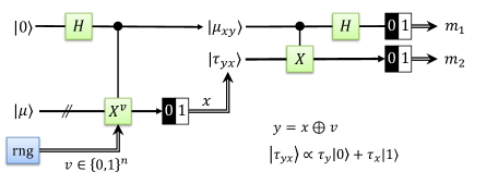
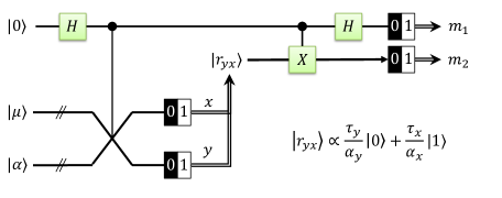
Figure 1: (top) A circuit to test an unknown quantum state $\mu$ with respect to a classically-described target state $\tau$. The circuit is repeated many times and the fidelity $F(\mu,\tau)$ between $\mu$ and $\tau$ is estimated in terms of weighted averages of $b=(-1)^{m_{1}}m_{2}$ and $b^{2}$ (eq. (4)). (bottom) An importance sampling circuit which reduces the number of circuit repetitions needed when $\tau$ is not anticoncentrated. Here $\alpha$ is any accurately-known state that samples $\mu$ and $\tau$ well. Notation: $H$ = Hadamard gate; $X$ = Pauli $X$ gate; 0/1 block = measurement in the computational basis; rng = random number generator.

II.2 Performance

II.2.1 Cost to Achieve a Given Precision

The cost of EVAQS is driven by the number of samples needed to obtain an estimate with sufficiently small variance. In a typical application the expectation is that $\mu$ is not a bad approximation of $\tau$; thus the regime of greatest interest is that of small infidelity $I\equiv 1-F$. To lowest order in $I$ and statistical fluctuations, the variance of $\tilde{F}$ can be written as

$$\operatorname{Var}\tilde{F} \approx\frac{2}{N}\sum_{x}\frac{I\left|\tau_{x}\right|^{4}+\left|\tau_{x}\right|^{2}\left|\epsilon_{x}\right|^{2}}{\left|\alpha_{x}\right|^{2}}.$$ (7)

where $\epsilon\equiv e^{-\mathrm{i}\phi}\mu-\tau$ is the error of $\mu$ upon correcting its global phase $\phi$, defined via $\langle\tau|\mu\rangle=\sqrt{F}e^{\mathrm{i}\phi}$ . As shown in the Appendix, $\left|\epsilon_{x}\right|^{2}$ is (to lowest order) also proprtional to $I$, so that the entire expression is proportional to $I$. Note that $\operatorname{Var}\tilde{F}$ does not depend on the phases of the components of $\alpha$.

The worst case is that the error $\epsilon$ resides entirely on the component $x$ for which $\left|\tau_{x}/\alpha_{x}\right|$ is largest, i.e. the basis state which is most badly undersampled. In non-adversarial scenarios the error may be expected to be distributed across the support of $\tau$. Simulations indicate that for plausible error models $\sum_{x}\left|\tau_{x}\right|^{2}\left|\epsilon_{x}\right|^{2}/\left|\alpha_{x}\right|^{2}$ is typically comparable in magnitude to $I\sum_{x}\left|\tau_{x}\right|^{4}/\left|\alpha_{x}\right|^{2}$. This leads to the scaling heuristic

$$N \sim\frac{4I}{\epsilon^{2}}\left(1+\chi^{2}(\left|\tau\right|^{2},\left|\alpha\right|^{2})\right)$$ (8)

where $\epsilon^{2}$ is the desired variance and $\chi^{2}(p,q)\equiv\sum_{x}\left|p_{x}-q_{x}\right|^{2}/q_{x}$ is the chi-square divergence of $p$ with respect to $q$. $\chi^{2}$ is a standard statistical measure that quantifies the “distance” between distributions $p$ and $q$, heavily weighting differences in which $q$ undersamples $p$. Note that $N$ has no intrinsic dependence on the dimension of $\tau$.

For the basic version of the algorithm (or when $\alpha$ is the uniform superposition), eq. (8) can be simplified even further to

$$N \sim\frac{4I}{\epsilon^{2}}dp_{\text{coll}}^{(\tau)}$$ (9)

where $p_{\text{coll}}^{(\tau)}=\sum_{x}\left|\tau_{x}\right|^{4}$ is the collision probability of the classical distribution induced by $\tau$. $1/p_{\text{coll}}^{(\tau)}$ may be interpreted as the effective support size $d_{\text{eff}}$ of $\tau$. It follows that the basic algorithm is efficient so long as $d_{\text{eff}}/d$ is at least $1/\text{poly}(n)$, that is, so long as the effective support of $\tau$ is not too small. This make the proposed method complementary to existing methods which are efficient for concentrated distributions. For a slightly different perspective, the factor $dp_{\text{coll}}^{(\tau)}$ can be written as $2^{n-H_{2}^{(\tau)}}$ where $H_{2}^{(\tau)}$ is the Rï¿œnyi 2-entropy of the classical distribution induced by $\tau$. Thus the basic method is efficient when the entropy is large, namely, when $n-H_{2}^{(\tau)}$ grows at most logarithmically in $n$.

Using standard calculus one can show that the optimal sampling distribution satisfies

$$\left|\alpha_{x}\right|^{2} \propto\sqrt{\left|\tau_{x}\right|^{2}\left(\left|\tau_{x}\right|^{2}+\left|\sigma_{x}\right|^{2}\right)}$$ (10)

where $\sigma$ is the normalized projection of $\epsilon$ onto the space orthogonal to $\tau$. One might have guessed that it would be sufficient for $\alpha$ to sample either $\mu$ or $\tau$ well. But that is incorrect: If $\alpha$ doesn’t frequently sample the components of $\mu$ with the largest errors (whether or not the components themselves are large), then the (in)fidelity will not be estimated with high precision.

II.2.2 Robustness to Error in the Auxiliary State

A key assumption in the general version of EVAQS is that the auxiliary state $\alpha$ is well-characterized. Fortunately, EVAQS is robust with respect to this assumption in the sense that small error in the knowledge of $\alpha$leads to a correspondingly small error in the estimate of $F(\mu,\tau)$.

Suppose $\alpha$ is mistakenly characterized as $\tilde{\alpha}$. Then as shown in Section III.3, instead of estimating $F(\mu,\tau)$ the procedure estimates $F(\mu,\tilde{\tau}$) where $\tilde{\tau}$ is a perturbed version of $\tau$, namely

$$\tilde{\tau}_{x} \equiv\frac{\tau_{x}\alpha_{x}/\tilde{\alpha}_{x}}{\sqrt{\sum_{y}\left|\tau_{y}\alpha_{y}/\tilde{\alpha}_{y}\right|^{2}}}.$$ (11)

Intuitively, if $\tilde{\alpha}$ is close to $\alpha$ then $\tilde{\tau}$ will be close to $\tau$ and $F(\mu,\tilde{\tau})$ will be close to $F(\mu,\tau)$. In Section III.3 and Appendix C it is shown that

$$F(\mu,\tau) \geq F(\mu,\tilde{\tau})-\frac{2\delta_{\text{rms}}}{1-\delta_{\text{rms}}}$$ (12)

where $\delta_{\text{rms}}$ is the average relative error in $\tilde{\alpha}$. Thus a small error in the characterization of $\alpha$ yields a correspondingly small error in the estimate of $F(\mu,\tau)$.

II.3 Simulations

In this section I present the results of several simulation studies demonstrating the validity and efficacy of the proposed method. The first study demonstrates scalable verification of so-called instantaneous quantum polynomial (IQP) circuits (Shepherd and Bremner, 2009). The next two studies demonstrate sample-efficient verification of random quantum circuits, including the kind of circuits used to demonstrate quantum supremacy (Arute et al., 2019). In each of these studies the basic version of the method (without an auxiliary state $|\alpha\rangle$) was employed.

II.3.1 Verification of IQP Circuits

IQP circuits are currently of interest as a family of relatively simple quantum circuits whose output distributions are hard to simulate classically (Bremner et al., 2011, 2016). IQP circuits are well-suited for demonstrating EVAQS as their outputs are typically anticoncentrated in the computational basis. Even better, if the output an IQP circuit is transformed into the Hadamard basis, the distribution is not only perfectly uniform (yielding the lowest possible sample complexity), but also easy to calculate on a classical computer. This makes EVAQS a fully scalable way to verify IQP circuits.

An $n$-qubit IQP circuit of depth $m$ can be defined as a set of $m$ multiqubit $X$ rotations acting on the $|0\rangle^{n}$ state. A multiqubit NOT operation may be written as $X^{a}\equiv X_{1}^{a_{1}}\otimes\cdots\otimes X_{n}^{a_{n}}$ for $a\in\{0,1\}^{n}$. In terms of such operators, an IQP circuit has the form

$$|\tau\rangle =\exp\left(\mathrm{i}\sum_{i=1}^{m}\theta_{i}X^{A_{i}}\right)|0\rangle^{n}.$$ (13)

for some set of vectors $A_{1},\ldots,A_{m}\in\{0,1\}^{n}$. The amplitudes of the output state can be written concisely as

$$\tau_{x} =\langle x|\tau\rangle$$ (14)

$$=\sum_{v:\leavevmode\nobreak\ Av=x}\beta_{1}(v_{1})\cdots\beta_{n}(v_{n})$$ (15)

where $A=[A_{1},\ldots,A_{m}]$ and

$$\beta_{i}(b) =\begin{cases}\cos\theta_{i}&b=0\\ \mathrm{i}\sin\theta_{i}&b=1\end{cases}.$$ (16)

The number of terms in $\sum_{v:\leavevmode\nobreak\ Av=x}$ is $2^{m-r}$ where $r=\operatorname{rank}(A)$. Since $r\leq n$, the number of terms contributing to $\tau_{x}$ is exponential in the circuit depth $m$ once it exceeds $n$.

In the Hadamard Basis

IQP states are substantially easier to analyze in the Hadamard basis. Let $|\xi\rangle=H^{\otimes n}|\tau\rangle$. Note that it is experimentally easy to obtain $|\xi\rangle$ from $|\tau\rangle$. Since $HX=ZH$, we have

$$|\xi\rangle =\exp\left(\mathrm{i}\sum_{i=1}^{m}\theta_{i}Z^{A_{i}}\right)|+\rangle^{n}$$ (17)

where $|+\rangle\equiv(|0\rangle+|1\rangle)/\sqrt{2}=H|0\rangle$. In this basis, the amplitude

$$\langle x|\xi\rangle =\frac{1}{\sqrt{2^{n}}}\exp\left(\mathrm{i}\sum_{i=1}^{m}\theta_{i}(-1)^{x\cdot A_{i}}\right)$$ (18)

is trivial to compute classically. Furthermore, the induced probability distribution is uniform, which is the best case for EVAQS.

As a first demonstration, I simulated the verification of random IQP circuits in the Hadamard basis. The test circuits were comprised of $n=4,6,8,\ldots,20$ qubits and $m=3n$ rotations; the depth $m=3n$ was chosen to ensure that the complexity of the output state is exponential in $n$. For each rotation, a random subset of qubits was chosen from $n$ Bernoulli trials such that on average 2 qubits were involved in each rotation. Each rotation angle was chosen uniformly from $[0,2\pi]$. To simulate circuit error, each angle $\theta_{i}$ was perturbed by a small random amount $\delta_{i}$. The angle errors were globally scaled so that the resulting state $|\mu\rangle$ had a prescribed infidelity $I$ with respect to the ideal state. For each $n$ and each $I\in\{0.01,0.03,0.1,0.3\}$, 400 random noisy circuits were realized. For each circuit, the verification procedure was performed with $10^{4}$ simulated measurements.

The left plot in Fig. 2 shows the estimated infidelities obtained from these simulated experiments. (In all the figures, a solid line shows the median value among all realizations of a given experiment and a surrounding shaded band shows the 10th-90th percentiles). As expected, the proposed method is able to accurately estimate the infidelity of the prepared state independent of number of qubits and over a wide range of infidelities. With a fixed number of measurements, the states with smaller infidelity are estimated with larger relative error; however, the absolute error is actually smaller, in accordance with eq. (9). The right panel of Fig. 2 shows the sample cost of the procedure, given by eq. (LABEL:eq:_true_variance) and normalized by the desired precision $\epsilon^{2}$, as a function of the number of qubits. Notably, the cost is independent of the number of qubits, depending only on the fidelity of the test state. Again, this is expected from eq. (9) given that the output distribution is uniform.

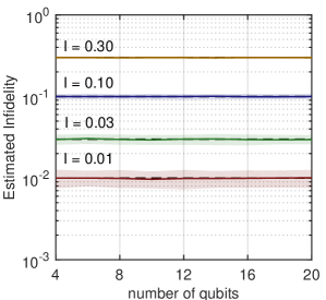
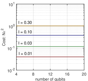
Figure 2: Simulated verification of IQP circuits with rotation angle errors, using measurements in the Hadamard basis. (left) Estimated infidelity. (right) Precision-normalized cost.

In the Computational Basis

EVAQS is also effective when measurements are performed in the computational basis. In this basis, the output state of a typical IQP circuit is anticoncentrated in the sense that significant fraction of the basis states have probabilities of order $2^{-n}$ or larger (Webb and Bennink, 2020). Fig. 3,left shows the estimated infidelities for the same set of circuits as described in the previous subsection, but this time using simulated measurements in the computational basis. As before, EVAQS was able to accurately estimate the circuit fidelities. This time, however, the cost tends to increase slowly with the number of qubits. I note that while the median cost does appear to grow exponentially, in going from 4 to 20 qubits it increases only by a factor of about 2.5, whereas the size of the state being verified increases by a factor of $2^{20}/2^{4}=65\thinspace 536$. Furthermore, there is noticeable variation in cost for circuits of the same size (Fig. 3, middle). This is because different random circuits of the same size were anticoncentrated to different degrees. The strong link between cost and the degree of anticoncentration in the target distribution is shown in Fig. 3,right. Indeed, the degree of concentration (as measured by the inverse collision probability) is a better predictor of cost than the number of qubits. Also noteworthy is the fact that the estimated costs, given by eq. (9) and shown as dashed lines, are within a small factor of the true costs.

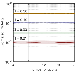
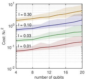
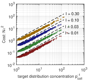
Figure 3: Simulated verification of IQP circuits with rotation angle errors, using measurements in the computational basis. (left) Estimated infidelity. (middle) Precision-normalized cost. (right) Cost as a function of the concentratedness of the output state. The dashed lines are the estimated cost, eq. (8).

II.3.2 Verification of Random Circuits

The second study involves verification of random quantum circuits, that is, sequences of random 2-qubit unitaries on randomly selected pairs of qubits. Each random unitary was obtained by generating a random complex matrix with normally-distributed elements, then performing Gram-Schmidt orthogonalization on the columns of the matrix. In this study, error was modelled as a perturbation of the output state rather than perturbation of the individual gates. The output state was written as

$$|\mu\rangle =\sqrt{1-\eta}|\tau\rangle+\sqrt{\eta}|\epsilon\rangle$$ (19)

where $|\epsilon\rangle$ consisted of both multiplicative and additive noise,

$$\epsilon_{x} \sim\xi_{x}^{\prime}\tau_{x}+\lambda\xi_{x}^{\prime\prime}$$ (20)

where $\xi_{x}^{\prime},\xi_{x}^{\prime\prime}$ are independent complex Gaussian random variables.The constant $\lambda$ was chosen so that the standard deviations of the multiplicative error and additive error are equal when $\left|\tau_{x}\right|$ equals its mean value. The constant $\eta$ was then chosen to yield a particular infidelity $I$. As before, circuits were comprised of $n=2,4,6,\ldots,20$ qubits and $m=3n$ gates. For each $n$ and $I\in\{0.01,0.03,0.1,0.3\}$, 300 random circuits were realized. For each circuit, the verification procedure was performed with $10^{4}$ simulated measurements.

The results are shown in Fig. 4. Again, EVAQS is able to estimate the output state fidelity accurately with a number of measurements that grows very slowly with the number of qubits. And as with IQP circuits, the cost is well-predicted by the concentration of the target state and the infidelity of the unknown state.

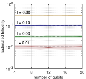
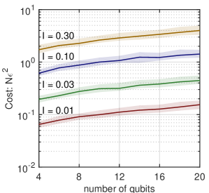
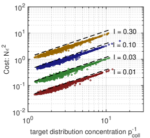
Figure 4: Simulated verification of quantum circuits consisting of random 2-qubit unitaries and random error on the output state. (left) Estimated infidelity. (middle) Precision-normalized cost. (right) Cost as a function of the concentratedness of the output state. The dashed lines are the estimated cost, eq. (8).

II.3.3 Verification of Supremacy Circuits

Another important class of circuits is that recently used to demonstrate the “quantum supremacy” of a quantum processor (Arute et al., 2019). Such circuits consist of alternating rounds of single-qubit rotations drawn from a small discrete set and entangling operations on adjacent pairs of qubits in a particular pattern. Like IQP circuits, such circuits are hard to classically simulate (Aaronson and Chen, 2016; Aaronson and Gunn, 2020) in spite of their locality constraints. But unlike IQP circuits, they are universal for quantum computing.

The circuits simulated in this study consisted of $n\in\{4,9,12,16,20\}$ qubits arranged in a planar square lattice with (nearly) equal sides and 16 cycles of alternating single-qubit operations and entangling operations, as described in (Arute et al., 2019). Single-qubit error was modelled as a post-operation unitary of the form $\exp\left(\mathrm{i}(\epsilon_{x}X+\epsilon_{y}Y+\epsilon_{z}Z\right)$ where $\epsilon_{x},\epsilon_{y},\epsilon_{z}$ are independent normally-distributed variables of zero mean and small variance. Error on the two-qubit operations was modelled as a small random perturbation of the angles $\theta,\phi$ parameterizing the entangling gate (Arute et al., 2019). The amount of error was chosen to yield a process infidelity (Gilchrist et al., 2005) on the order of 0.02% per single-qubit operation and 0.2% per two-qubit operation. For each circuit size, 100 random noisy circuits were generated; for each circuit, $10^{4}$measurements were simulated.

Fig. 5 plots the estimated fidelity vs. the true infidelity of all the circuits simulated. For comparison, the dashed line shows the true infidelity. The smallest circuits ($n=4$) had output infidelities on the order of $10^{-3}$, while the largest ($n=20$) had infidelities around 0.3. Over this range, the infidelity was estimated to within 20% or better. What is not evident from the plot is that the variance of the estimator varied by an order of magnitude for different random circuits of the same size, due to the different amounts of entropy in their output distributions. Consequently, the expected error for some of the circuits is actually considerably smaller than 20%. For the circuits that were verified less accurately, the expected error could be reduced further by increasing the number of measurements. Interestingly, the relative error does not vary much over the wide range of circuit sizes and circuit infidelities in these simulations. According to eq. (9), one expects the relative error to scale as $\sqrt{\operatorname{Var}\tilde{F}}/I\propto I^{-1/2}$, that is, to increase as infidelity decreases. Additional simulations confirmed that this scaling does occur with smaller gate errors.

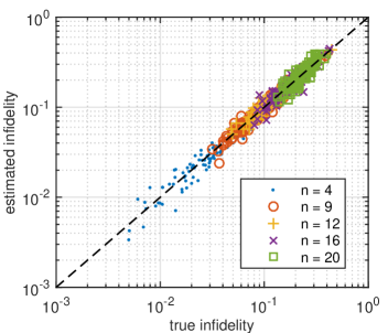
Figure 5: (color online) Simulated verification of the types of circuits used in recent quantum supremacy demonstrations. $n$ is the number qubits.

III Methods

III.1 Proof of Correctness

To see that the procedures described in Section II.1 indeed yield an estimate of $F(\mu,\tau)$, let us consider the general case first; the correctness of the simpler version will then be established as a special case.

III.1.1 Proof of General Version

In each iteration of the general algorithm, one first prepares the test register, auxiliary register, and the first ancilla qubit in the state

$$|\psi\rangle =\frac{1}{\sqrt{2}}|\mu\rangle|\alpha\rangle(|0\rangle+|1\rangle)$$ (21)

$$=\frac{1}{\sqrt{2}}\sum_{x,y=1}^{d}\mu_{x}\alpha_{y}|x\rangle|y\rangle(|0\rangle+|1\rangle).$$ (22)

In the second step, the ancilla controls a swap between the test and auxiliary registers. This yields the state

$$|\psi^{\prime}\rangle =\frac{1}{\sqrt{2}}\sum_{x,y=1}^{d}|x\rangle|y\rangle(\mu_{x}\alpha_{y}|0\rangle+\mu_{y}\alpha_{x}|1\rangle).$$ (23)

In the third step the test and auxiliary registers are measured, yielding values $x,y$. This projects ancilla 1 onto the unnormalized state

$$|\psi_{xy}\rangle =\frac{1}{\sqrt{2}}(\mu_{x}\alpha_{y}|0\rangle+\mu_{y}\alpha_{x}|1\rangle).$$ (24)

In the fourth step, the observed values $x,y$ are used to compute $\tau_{x}^{\prime},\tau_{y}^{\prime},\alpha_{x}^{\prime},\alpha_{y}^{\prime}$ and prepare ancilla qubit 2 in the state

$$|r_{yx}\rangle \equiv\frac{1}{\sqrt{w_{yx}^{\prime}}}\left(\frac{\tau_{y}^{\prime}}{\alpha_{y}^{\prime}}|0\rangle+\frac{\tau_{x}^{\prime}}{\alpha_{x}^{\prime}}|1\rangle\right).$$ (25)

Let $\lambda=\left|\tau_{x}^{\prime}/\tau{}_{x}\right|^{2}/\left|\alpha_{x}^{\prime}/\alpha_{x}\right|^{2}$, which is independent of $x$. Then $|r_{yx}\rangle$ can be written as

$$|r_{yx}\rangle =\frac{1}{\sqrt{w_{yx}}}\left(\frac{\tau_{y}}{\alpha_{y}}|0\rangle+\frac{\tau_{x}}{\alpha_{x}}|1\rangle\right)$$ (26)

where $w_{xy}=w_{xy}^{\prime}/\lambda$. The joint state of the two ancillas is

$$|\psi_{xy}^{\prime}\rangle =\frac{1}{\sqrt{2w_{xy}}}\left(\mu_{x}\alpha_{y}|0\rangle+\mu_{y}\alpha_{x}|1\rangle\right)\left(\frac{\tau_{y}}{\alpha_{y}}|0\rangle+\frac{\tau_{x}}{\alpha_{x}}|1\rangle\right)$$ (27)

Finally, the ancillas are measured in the Bell basis. Since

$$\langle\Phi_{\pm}|\psi_{xy}^{\prime}\rangle =\frac{1}{\sqrt{2w_{xy}}}\left(\mu_{x}\tau_{y}\pm\mu_{y}\tau_{x}\right)$$ (28)

the probability of outcome $b=\pm 1$ is

$$p_{x,y,\pm 1} =\frac{1}{4w_{xy}}\left(\left|\mu_{x}\right|^{2}\left|\tau_{y}\right|^{2}+\left|\mu_{y}\right|^{2}\left|\tau_{x}\right|^{2}\pm\mu_{x}\tau_{y}\mu_{y}^{*}\tau_{x}^{*}\pm\mu_{y}\tau_{x}\mu_{x}^{*}\tau_{y}^{*}\right).$$ (29)

Using $\left|\sum_{x}\mu_{x}^{*}\tau_{x}\right|^{2}=F(\mu,\tau)$ we obtain

$$\sum_{x,y}w_{xy}p_{xy\pm} =\frac{1}{2}\left(1\pm F(\mu,\tau)\right).$$

Now, $p_{xy+}+p_{xy-}=\sum_{b\in\{-1,0,1\}}p_{xyb}b^{2}$ and $p_{xy+}-p_{xy-}=\sum_{b\in\{-1,0,1\}}p_{xyb}b$. Thus

$$\left<w_{xy}^{\prime}b\right> =\lambda\sum_{x,y,b}w_{xy}p_{xyb}b$$ (30)

$$=\lambda\sum_{x,y}w_{xy}(p_{xy+}-p_{xy-})$$ (31)

$$=\lambda F(\mu,\tau)$$ (32)

and

$$\left<w_{xy}^{\prime}b^{2}\right> =\lambda\sum_{x,y,b}w_{xy}p_{xyb}b^{2}$$ (33)

$$=\lambda\sum_{x,y}w_{xy}(p_{xy+}+p_{xy-})$$ (34)

$$=\lambda.$$ (35)

Thus

$$F(\mu,\tau) =\frac{\left<w_{xy}^{\prime}b\right>}{\left<w_{xy}^{\prime}b^{2}\right>}.$$ (36)

To obtain an experimental estimate of $F(\mu,\tau)$, the steps above are repeated $N\gg 1$ times. Let $x_{i},y_{i},b_{i}$ denote the values of $x,y,b$ obtained in the $i$th trial. Let $A_{i}=w_{x_{i}y_{i}}^{\prime}b_{i}$ and $B_{i}=w_{x_{i}y_{i}}^{\prime}b_{i}^{2}$. The experimental quantities

$$\tilde{A} \equiv\frac{1}{N}\sum_{i=1}^{N}A_{i}$$ (37)

$$\tilde{B} \equiv\frac{1}{N}\sum_{i=1}^{N}B_{i}$$ (38)

are unbiased estimators of $A=\lambda F$ and $B=\lambda$ respectively. As a first approximation $F$ may be estimated by the ratio $\tilde{A}/\tilde{B}$. It is a basic result of statistical analysis that such an estimator has a bias of order $N^{-1}$. The estimator which corrects for this bias is derived in Appendix A.

III.1.2 Proof of the Basic Version

To establish the correctness of the basic version of the algorithm, I show that it is equivalent to performing the general algorithm with $\alpha$ as the uniform superposition state.

In the basic version, one starts with just the unknown state $|\mu\rangle$ and an ancilla qubit in the state $(|0\rangle+|1\rangle)/\sqrt{2}$. One picks a uniform random vector $v\in\{0,1\}^{n}$ and performs

$$|x\rangle|0\rangle \rightarrow|x\rangle|0\rangle$$ (39)

$$|x\rangle|1\rangle \rightarrow|x\oplus v\rangle|1\rangle$$ (40)

yielding the state

$$|\psi_{xy,x\oplus v}^{\prime}\rangle =\frac{1}{\sqrt{2}}\sum_{x}\mu_{x}\left(|x\rangle|0\rangle+|x\oplus v\rangle|1\rangle\right)$$ (41)

$$=\frac{1}{\sqrt{2}}\sum_{x}|x\rangle\left(\mu_{x}|0\rangle+\mu_{x\oplus v}|1\rangle\right).$$ (42)

Measuring $x$ yields the ancilla state

$$\mu_{x}|0\rangle+\mu_{x\oplus v}|1\rangle$$ (43)

with net probability

$$p_{x,v} =\frac{1}{2^{n+1}}\left(\left|\mu_{x}\right|^{2}+\left|\mu_{x\oplus v}\right|^{2}\right).$$ (44)

Now, consider the general algorithm with $|\alpha\rangle=2^{-n/2}\sum_{y}|y\rangle$. From eq. (23), the state immediately following the controlled swap between test and auxiliary registers is

$$|\psi^{\prime}\rangle =\frac{1}{\sqrt{2^{n+1}}}\sum_{x,y}|x\rangle|y\rangle(\mu_{x}|0\rangle+\mu_{y}|1\rangle).$$ (45)

Measurement of $x,y$ yields the ancilla state

$$\mu_{x}|0\rangle+\mu_{y}|1\rangle$$ (46)

with probability

$$p_{xy} =\frac{1}{2^{n+1}}\left(\left|\mu_{x}\right|^{2}+\left|\mu_{y}\right|^{2}\right).$$ (47)

Eqs. (46),(47) are the same as $(\ref{eq: ancilla state (RNG)}$),(44). Thus, the basic version of the algorithm is equivalent to the general version with a uniform superposition for $\alpha$.

III.2 Derivation of the Variance

The cost of EVAQS is driven by the number of samples needed to obtain an estimate with sufficiently small variance. In Appendix B is is shown that, to lowest order in statistical fluctuations,

$$\operatorname{Var}\tilde{F} \approx\frac{1}{N}\sum_{x}\frac{\left|\tau_{x}\right|^{2}}{\left|\alpha_{x}\right|^{2}}Q_{x}$$ (48)

where

$$Q_{x} \equiv(1+F^{2})\left(\left|\mu_{x}\right|^{2}+\left|\tau_{x}\right|^{2}\right)-2F\left(\tau_{x}^{*}\mu_{x}\langle\mu|\tau\rangle+\tau_{x}\mu_{x}^{*}\langle\tau|\mu\rangle\right).$$ (49)

In a typical application the expectation is that $\mu$ is not a bad approximation of $\tau$; thus the regime of interest is that of small infidelity $I\equiv 1-F$. We proceed to simplify $Q_{x}$ for the case that the infidelity $I\equiv 1-F$ is small, keeping only the lowest order terms. Let $\langle\tau|\mu\rangle=e^{\mathrm{i}\phi}\cos\theta$. Then $F=\cos^{2}\theta$, $I=\sin^{2}\theta$, and $1+F^{2}\approx 2F$. This yields

$$Q_{x} \approx 2F\left(\left|\mu_{x}\right|^{2}+\left|\tau_{x}\right|^{2}-\cos\theta\left(\tau_{x}\mu_{x}^{*}e^{\mathrm{i}\phi}+\tau_{x}^{*}\mu_{x}e^{-\mathrm{i}\phi}\right)\right).$$ (50)

Now, $\mu$ can be written as $\mu=e^{\mathrm{i}\phi}(\tau\cos\theta+\sigma\sin\theta)$ where $\left\|\sigma\right\|^{2}=1$ and $\langle\sigma|\tau\rangle=0$. Then $\tau_{x}^{*}\mu_{x}e^{-\mathrm{i}\phi}=\left|\tau_{x}\right|^{2}\cos\theta+\tau_{x}^{*}\sigma_{x}\sin\theta$. To lowest order in $\sin\theta=\sqrt{I}$,

$$\left|\mu_{x}\right|^{2} =\cos^{2}\theta\left|\tau_{x}\right|^{2}+\left|\sigma_{x}\right|^{2}\sin^{2}\theta+\cos\theta\sin\theta\left(\tau_{x}\sigma_{x}^{*}+\tau_{x}^{*}\sigma_{x}\right).$$ (51)

Substituting these expressions into (50) and combining terms yields

$$Q_{x} \approx 2F\left((1-\cos^{2}\theta)\left|\tau_{x}\right|^{2}+\left|\sigma_{x}\right|^{2}\sin^{2}\theta\right)$$ (52)

$$=2I\left(\left|\tau_{x}\right|^{2}+\left|\sigma_{x}\right|^{2}\right).$$ (53)

This yields

$$\operatorname{Var}\tilde{F} \approx\frac{2I}{N}\sum_{x}\frac{\left|\tau_{x}\right|^{2}\left(\left|\tau_{x}\right|^{2}+\left|\sigma_{x}\right|^{2}\right)}{\left|\alpha_{x}\right|^{2}}.$$ (54)

To obtain eq. (7, we combine the definitions $\mu=e^{\mathrm{i}\phi}(\tau\cos\theta+\sigma\sin\theta)$ and $\epsilon\equiv e^{-\mathrm{i}\phi}\mu-\tau$ to obtain

$$\epsilon =\tau(\cos\theta-1)+\sigma\sin\theta.$$ (55)

Since $(I-\tau\tau^{\dagger})\epsilon=\sigma\sin\theta$, $\sigma$ can be understood as the normalized projection of $\epsilon$ onto the subspace orthogonal to $\tau$. Alternatively, we may use the fact that $\sin\theta=\sqrt{1-F}=\sqrt{I}$ and $\cos\theta=\sqrt{F}\approx 1-\frac{1}{2}I$ to obtain

$$\epsilon \approx\sigma\sqrt{I}.$$ (56)

Eq. (7) follows from substituting this expression into (54).

III.3 Derivation of the Robustness Bound

Suppose $\alpha$ is mischaracterized as $\tilde{\alpha}$. Then upon measuring $x,y$ one is led to prepare the ancilla state

$$|\tilde{r}_{yx}\rangle \left(\frac{\tau_{y}}{\tilde{\alpha}_{y}}|0\rangle+\frac{\tau_{x}}{\tilde{\alpha}_{x}}|1\rangle\right)$$ (57)

and eq. (27) becomes

$$|\tilde{\psi}_{xy}^{\prime}\rangle =\frac{1}{\sqrt{2w_{xy}}}\left(\mu_{x}\alpha_{y}|0\rangle+\mu_{y}\alpha_{x}|1\rangle\right)\left(\frac{\tau_{y}}{\tilde{\alpha}_{y}}|0\rangle+\frac{\tau_{x}}{\tilde{\alpha}_{x}}|1\rangle\right).$$ (58)

The projection of the ancillas onto the Bell state $|\Phi_{\pm}\rangle$ is

$$\frac{1}{\sqrt{4w_{xy}}}\left(\mu_{x}\tau_{y}\frac{\alpha_{y}}{\tilde{\alpha}_{y}}\pm\mu_{y}\tau_{x}\frac{\alpha_{x}}{\tilde{\alpha}_{x}}\right).$$ (59)

Comparing this with (28) shows that $\tau$ is effectively replaced by $\tilde{\tau}$, where

$$\tilde{\tau}_{x} \equiv\frac{\tau_{x}\alpha_{x}/\tilde{\alpha}_{x}}{\sqrt{\sum_{y}\left|\tau_{y}\alpha_{y}/\tilde{\alpha}_{y}\right|^{2}}}.$$ (60)

That is, error in one’s knowledge of the auxiliary state $\alpha$ causes the algorithm to estimate the fidelity of $\mu$ with respect to a perturbed version of the target state. Intuitively, if $\tilde{\alpha}$ is close to $\alpha$ then $\tilde{\tau}$ will be close to $\tau$ and $F(\mu,\tilde{\tau})$ will be close to $F(\mu,\tau)$. To make this more precise we use the triangle inequality

$$\sqrt{1-F(\mu,\tau)} \leq\sqrt{1-F(\mu,\tilde{\tau})}+\sqrt{1-F(\tau,\tilde{\tau})}$$ (61)

from which it follows that

$$F(\mu,\tau) \geq F(\mu,\tilde{\tau})-2\sqrt{1-F(\tau,\tilde{\tau})}.$$ (62)

In Appendix C it is shown that

$$1-F(\tau,\tilde{\tau}) \leq\frac{\delta_{\text{rms}}^{2}}{(1-\delta_{\text{rms}})^{2}}$$ (63)

where $\delta_{\text{rms}}$ is the average relative error of $\tilde{\alpha}$, defined as

$$\delta_{\text{rms}}^{2} \equiv\sum_{x}\left|\tau_{x}\right|^{2}\left|\frac{\alpha_{x}}{\tilde{\alpha}_{x}}-1\right|^{2}.$$ (64)

Combining this with (62) yields the robustness bound (12).

IV Conclusion

The verification of complex states produced by quantum computers presents daunting experimental and computational challenges. In this paper I presented EVAQS, a novel state verification method that takes a significant step in addressing these challenges. In this method, a preparable quantum state is verified against a classical specification using a combination of relatively simple quantum circuits and on-the-fly calculations on a conventional computer. In contrast to existing verification methods, EVAQS is inherently sample-efficient when the target state is anticoncentrated (i.e., has high entropy) in the chosen measurement basis. In the case that the target state is not anticoncentrated, an auxiliary state may be used to importance sample the unknown state, greatly reducing the number of measurements needed.

The main limitation of EVAQS is the need to calculate selected probability amplitudes of the target state for comparison to the unknown state. If the state is not too large (say, less than 30 qubits), the probability amplitudes may feasibly be calculated ahead of time and stored in a look-up table for retrieval during verification. In the hopes of reducing the complexity of classical computation in some cases, the method was formulated in such a way that the calculated amplitudes need not be normalized. But if the task is to verify a quantum state against a classical specification, it seems there is no way to avoid the need to calculate characteristic features of the target state. Addressing this computational challenge to quantum state verification remains an important direction for future work.

EVAQS complements previously known verification methods that are efficient when the target state is sparse in some readily measurable basis. However, there exist interesting quantum states that are neither sparse nor anticoncentrated; for example, coherent analogs of thermal states at moderate temperatures. Such a state can have an effective support that is exponentially large (making it challenging for sparse methods) but still exponentially smaller than the number of basis states (making it challenging for EVAQS). Other approaches, perhaps yet to be discovered, will be needed to efficiently verify such states.

V Acknowledgments

This work was performed at Oak Ridge National Laboratory, operated by UT-Battelle, LLC under contract DE-AC05-00OR22725 for the US Department of Energy (DOE). Support for the work came from the DOE Advanced Scientific Computing Research (ASCR) Quantum Testbed Pathfinder Program under field work proposal ERKJ332.

Appendix A Correction of Residual Bias

To lowest order in statistical fluctuations,

$$\left<\frac{\tilde{A}}{\tilde{B}}\right>\approx F \left(1+\frac{\operatorname{Cov}(\tilde{A},\tilde{B})}{AB}-\frac{\operatorname{Var}\tilde{B}}{B^{2}}\right).$$ (65)

Thus

$$\frac{\tilde{A}}{\tilde{B}}\left(1-\frac{\operatorname{Cov}(\tilde{A},\tilde{B})}{AB}+\frac{\operatorname{Var}\tilde{B}}{B^{2}}\right)$$

is an estimator of $F$ in which the lowest order bias ($N^{-1}$) has been eliminated. The quantities appearing in the correction terms are unknown, but they can be estimated to the same order of accuracy as the estimator itself:

$$\frac{\operatorname{Var}\tilde{B}}{B^{2}} \approx\frac{1}{N(N-1)}\sum_{i}\left(\frac{B_{i}}{\tilde{B}}-1\right)^{2}$$ (66)

$$\frac{\operatorname{Cov}(\tilde{A},\tilde{B})}{AB} \approx\frac{1}{N(N-1)}\sum_{i}\left(\frac{A_{i}}{\tilde{A}}-1\right)\left(\frac{B_{i}}{\tilde{B}}-1\right).$$ (67)

This yields the improved estimator of $F$,

$$\tilde{F} \equiv\frac{\tilde{A}}{\tilde{B}}\left(1+\tilde{C}\right)$$ (68)

where

$$\tilde{C} =\frac{1}{N(N-1)}\sum_{i}\left(\frac{B_{i}}{\tilde{B}}-\frac{A_{i}}{\tilde{A}}\right)\left(\frac{B_{i}}{\tilde{B}}-1\right).$$ (69)

Appendix B Evaluation of Some Expectation Values

The variance of $\tilde{F}$ is a function of several different expectation values, which are here identified and evaluated. To lowest order in statistical fluctuations, the variance of $\tilde{F}$ is

$$\operatorname{Var}\tilde{F} =\operatorname{Var}\frac{\tilde{A}}{\tilde{B}}$$ (70)

$$\approx\frac{\langle\tilde{A}\rangle^{2}}{\langle\tilde{B}\rangle^{2}}\operatorname{Var}\left(\frac{\tilde{A}}{\langle\tilde{A}\rangle}-\frac{\tilde{B}}{\langle\tilde{B}\rangle}\right).$$ (71)

With the relations $\left<\tilde{A}\right>=\lambda F$ and $\left<\tilde{B}\right>=\lambda$ this simplifies to

$$\operatorname{Var}\tilde{F} \approx F^{2}\operatorname{Var}\left(\frac{\tilde{A}}{\lambda F}-\frac{\tilde{B}}{\lambda}\right)$$ (72)

$$=\operatorname{Var}\left(\frac{1}{\lambda}\left(\tilde{A}-\tilde{B}F\right)\right)$$ (73)

$$=\frac{1}{\lambda^{2}}\left(\left<\left(\tilde{A}-\tilde{B}F\right)^{2}\right>-\left<\tilde{A}-\tilde{B}F\right>^{2}\right).$$ (74)

Now, $\left<\tilde{A}-\tilde{B}F\right>=0$. To evaluate $\left<\left(\tilde{A}-\tilde{B}F\right)^{2}\right>$ we use (37) and (38) to write

$$\tilde{A}-\tilde{B}F =\frac{\lambda}{N}\sum_{i=1}^{N}w_{x_{i}.y_{i}}\left(b_{i}-b_{i}^{2}F\right)$$ (75)

$$\equiv\frac{\lambda}{N}\sum_{i=1}^{N}G_{i}$$ (76)

where each $G_{i}=w_{x_{i}.y_{i}}\left(b_{i}-b_{i}^{2}F\right)$ is an independent random variable with mean 0. Then

$$\operatorname{Var}\tilde{F} \approx\frac{1}{N^{2}}\sum_{i,j=1}^{N}\left<G_{i}G_{j}\right>$$ (77)

$$=\frac{1}{N^{2}}\sum_{i=1}^{N}\left<G_{i}^{2}\right>$$ (78)

$$=\frac{1}{N}\left<w_{xy}^{2}(b-b^{2}F)^{2}\right>.$$ (79)

Using $b^{3}=b$ and $b^{4}=b^{2}$ we obtain

$$\operatorname{Var}\tilde{F} \approx\frac{1+F^{2}}{N}\left<w_{xy}^{2}b^{2}\right>-\frac{2F}{N}\left<w_{xy}^{2}b\right>.$$ (80)

Now,

$$\left<w_{xy}^{2}b^{2}\right> =\sum_{x,y,b}w_{xy}^{2}p_{xyb}b^{2}$$ (81)

$$=\frac{1}{2}\sum_{x,y}\left(\frac{\left|\tau_{x}\right|^{2}}{\left|\alpha_{x}\right|^{2}}+\frac{\left|\tau_{y}\right|^{2}}{\left|\alpha_{y}\right|^{2}}\right)\left(\left|\mu_{x}\right|^{2}\left|\tau_{y}\right|^{2}+\left|\mu_{y}\right|^{2}\left|\tau_{x}\right|^{2}\right)$$ (82)

$$=\sum_{x}\frac{\left|\tau_{x}\right|^{2}}{\left|\alpha_{x}\right|^{2}}\left(\left|\mu_{x}\right|^{2}+\left|\tau_{x}\right|^{2}\right)$$ (83)

and

$$\left<w_{xy}^{2}b\right> =\sum_{x,y,b}w_{xy}^{2}p_{xyb}b$$ (84)

$$=\frac{1}{2}\sum_{x,y}\left(\frac{\left|\tau_{x}\right|^{2}}{\left|\alpha_{x}\right|^{2}}+\frac{\left|\tau_{y}\right|^{2}}{\left|\alpha_{y}\right|^{2}}\right)\left(\mu_{x}\tau_{y}\mu_{y}^{*}\tau_{x}^{*}+\mu_{y}\tau_{x}\mu_{x}^{*}\tau_{y}^{*}\right)$$ (85)

$$=\sum_{x}\frac{\left|\tau_{x}\right|^{2}}{\left|\alpha_{x}\right|^{2}}\left(\tau_{x}^{*}\mu_{x}\langle\mu|\tau\rangle+\tau_{x}\mu_{x}^{*}\langle\tau|\mu\rangle\right).$$ (86)

This gives

$$\operatorname{Var}\tilde{F} \approx\frac{1}{N}\sum_{x}\frac{\left|\tau_{x}\right|^{2}}{\left|\alpha_{x}\right|^{2}}Q_{x}$$ (87)

where $Q_{x}$ is given by eq. (49).

Appendix C A Bound for the Robustness Result

In section II.2.2 it was shown that error in the auxiliary state $\alpha$ translates to an effective error in the target state $\tau$. In this section I bound the impact of such error on the estimated fidelity. Let $p$ denote the probability distribution induced by $\tau$, i.e. $p_{x}=\left|\tau_{x}\right|^{2}$. Let $\delta$, defined via $\alpha_{x}/\tilde{\alpha}_{x}=1+\delta_{x}$, quantify the error in the auxiliary state. In terms of these quantities $F(\tau,\tilde{\tau})$ can be written as

$$F(\tau,\tilde{\tau}) =\frac{\left|\sum_{x}p_{x}(1+\delta_{x})\right|^{2}}{\sum_{x}p_{x}\left|1+\delta_{x}\right|^{2}}$$ (88)

$$=\frac{\left|\left<1+\delta_{x}\right>\right|^{2}}{\left<\left|1+\delta_{x}\right|^{2}\right>}$$ (89)

where expectations are taken with respect to $p$. Then

$$1-F(\tau,\tilde{\tau}) =1-\frac{\left|\left<1+\delta_{x}\right>\right|^{2}}{\left<\left|1+\delta_{x}\right|^{2}\right>}$$ (90)

$$=\frac{\left<\left|1+\delta_{x}\right|^{2}\right>-\left|\left<1+\delta_{x}\right>\right|^{2}}{\left<\left|1+\delta_{x}\right|^{2}\right>}$$ (91)

$$=\frac{\operatorname{Var}\left(1+\delta_{x}\right)}{\left<\left|1+\delta\right|^{2}\right>}.$$ (92)

An upper bound on the numerator is

$$\operatorname{Var}\left(1+\delta_{x}\right) =\operatorname{Var}\delta_{x}\leq\delta_{\text{rms}}^{2}$$ (93)

where $\delta_{\text{rms}}\equiv\left<\left|\delta_{x}\right|^{2}\right>^{\frac{1}{2}}$. For the denominator, non-negativity of variance gives

$$\left<\left|1+\delta_{x}\right|^{2}\right> \geq\left|\left<1+\delta_{x}\right>\right|^{2}.$$ (94)

Now, $\left|1+\left<\delta_{x}\right>\right|\geq 1-\left|\left<\delta_{x}\right>\right|$. This time non-negativity of variance gives $\left|\left<\delta_{x}\right>\right|\leq\delta_{\text{rms}}$, hence

$$\left|1+\left<\delta_{x}\right>\right| \geq 1-\delta_{\text{rms}}.$$ (95)

The upper bound on the numerator combined with the lower bound on the denominator yields

$$1-F(\tau,\tilde{\tau}) \leq\frac{\delta_{\text{rms}}^{2}}{(1-\delta_{\text{rms}})^{2}}.$$ (96)

References

- Georgescu et al. (2014) I. M. Georgescu, S. Ashhab, and F. Nori, Rev. Mod. Phys. 86, 153 (2014), ISSN 0034-6861, 1539-0756.
- Tacchino et al. (2020) F. Tacchino, A. Chiesa, S. Carretta, and D. Gerace, Adv. Quantum Technol. 3, 1900052 (2020).
- Biamonte et al. (2017) J. Biamonte, P. Wittek, N. Pancotti, P. Rebentrost, N. Wiebe, and S. Lloyd, Nature 549, 195 (2017), ISSN 0028-0836, 1476-4687.
- Benedetti et al. (2019) M. Benedetti, E. Lloyd, S. Sack, and M. Fiorentini, Quantum Sci. Technol. 5, 019601 (2019), ISSN 2058-9565.
- Arute et al. (2019) F. Arute, K. Arya, R. Babbush, D. Bacon, J. C. Bardin, R. Barends, R. Biswas, S. Boixo, F. G. S. L. Brandao, D. A. Buell, et al., Nature 574, 505 (2019), ISSN 0028-0836, 1476-4687.
- Buhrman et al. (2001) H. Buhrman, R. Cleve, J. Watrous, and R. de Wolf, Phys. Rev. Lett. 87, 167902 (2001).
- Shabani et al. (2011) A. Shabani, R. L. Kosut, M. Mohseni, H. Rabitz, M. A. Broome, M. P. Almeida, A. Fedrizzi, and A. G. White, Phys. Rev. Lett. 106, 100401 (2011), ISSN 0031-9007, 1079-7114.
- Jiying et al. (2010) L. Jiying, Z. Jubo, L. Chuan, and H. Shisheng, Opt. Lett. 35, 1206 (2010), ISSN 0146-9592, 1539-4794.
- Howland et al. (2016) G. A. Howland, S. H. Knarr, J. Schneeloch, D. J. Lum, and J. C. Howell, Phys. Rev. X 6, 021018 (2016), ISSN 2160-3308.
- Ahn et al. (2019) D. Ahn, Y. S. Teo, H. Jeong, F. Bouchard, F. Hufnagel, E. Karimi, D. Koutný, J. Řeháček, Z. Hradil, G. Leuchs, et al., Phys. Rev. Lett. 122, 100404 (2019), ISSN 0031-9007, 1079-7114.
- Bairey et al. (2019) E. Bairey, I. Arad, and N. H. Lindner, Phys. Rev. Lett. 122, 020504 (2019), ISSN 0031-9007, 1079-7114.
- Flammia and Liu (2011) S. T. Flammia and Y.-K. Liu, Phys. Rev. Lett. 106, 230501 (2011), ISSN 0031-9007, 1079-7114.
- da Silva et al. (2011) M. P. da Silva, O. Landon-Cardinal, and D. Poulin, Phys. Rev. Lett. 107, 210404 (2011), ISSN 0031-9007, 1079-7114.
- Valiant and Valiant (2014) G. Valiant and P. Valiant, in 2014 IEEE 55th Annual Symposium on Foundations of Computer Science (2014), pp. 51–60, ISSN 0272-5428.
- Huang et al. (2020) H.-Y. Huang, R. Kueng, and J. Preskill, arXiv:2002.08953 [quant-ph] (2020), eprint 2002.08953.
- Buhrman et al. (2006) H. Buhrman, R. Cleve, M. Laurent, N. Linden, A. Schrijver, and F. Unger, in 2006 47th Annual IEEE Symposium on Foundations of Computer Science (FOCS’06) (IEEE, Berkeley, CA, USA, 2006), pp. 411–419, ISBN 978-0-7695-2720-8.
- Smolin and DiVincenzo (1996) J. A. Smolin and D. P. DiVincenzo, Phys. Rev. A 53, 2855 (1996).
- Hung et al. (2006) W. Hung, Xiaoyu Song, Guowu Yang, Jin Yang, and M. Perkowski, IEEE Trans. Comput.-Aided Des. Integr. Circuits Syst. 25, 1652 (2006), ISSN 0278-0070.
- Shepherd and Bremner (2009) D. Shepherd and M. J. Bremner, Proc. R. Soc. A 465, 1413 (2009), ISSN 1364-5021, 1471-2946, eprint 0809.0847.
- Bremner et al. (2011) M. J. Bremner, R. Jozsa, and D. J. Shepherd, Proc. R. Soc. A 467, 459 (2011), ISSN 1364-5021, 1471-2946.
- Bremner et al. (2016) M. J. Bremner, A. Montanaro, and D. J. Shepherd, Phys. Rev. Lett. 117, 080501 (2016).
- Webb and Bennink (2020) Z. Webb and R. S. Bennink (2020).
- Aaronson and Chen (2016) S. Aaronson and L. Chen, 200, 66 (2016).
- Aaronson and Gunn (2020) S. Aaronson and S. Gunn, arXiv:1910.12085 [quant-ph] (2020), eprint 1910.12085.
- Gilchrist et al. (2005) A. Gilchrist, N. K. Langford, and M. A. Nielsen, Phys. Rev. A 71, 062310 (2005), ISSN 1050-2947, 1094-1622.