Rule Extraction from Binary Neural Networks with Convolutional Rules for Model Validation

Abstract

Most deep neural networks are considered to be black boxes, meaning their output is hard to interpret. In contrast, logical expressions are considered to be more comprehensible since they use symbols that are semantically close to natural language instead of distributed representations. However, for high-dimensional input data such as images, the individual symbols, i.e. pixels, are not easily interpretable. We introduce the concept of first-order convolutional rules, which are logical rules that can be extracted using a convolutional neural network (CNN), and whose complexity depends on the size of the convolutional filter and not on the dimensionality of the input. Our approach is based on rule extraction from binary neural networks with stochastic local search. We show how to extract rules that are not necessarily short, but characteristic of the input, and easy to visualize. Our experiments show that the proposed approach is able to model the functionality of the neural network while at the same time producing interpretable logical rules.

Keywords— k-term DNF, stochastic local search, convolutional neural networks, logical rules, rule extraction, interpretability

1 Introduction

Neural Networks (NNs) are commonly seen as black boxes, which makes their application in some areas still problematic (e.g., in safety-critical applications or applications in which DL is intended to support communication with a human user). Logical statements, however, are arguably much easier to grasp by humans than the main building blocks of NNs (e.g., nonlinearities, matrix multiplications, or convolutions). In general, learning of logical rules cannot be done using gradient-based algorithms as they are not differentiable. Even if we find rules that exactly describe a neural network, they might still be too complex to be understandable. To solve this problem, we propose convolutional rules for which the complexity is not related to the dimensionality of the input but only to the dimensionality of the convolutional filters.

It is a wide-spread belief that shorter rules are usually better than longer rules, a principle known as Occam’s razor. This common assumption was recently challenged again by Stecher et al. (2016), who revive the notion of so-called characteristic rules instead. As they show, shorter rules are often discriminative rules that help to differentiate different output classes, but are not necessarily descriptive of the data. In this work, we can confirm this observation and show how characteristic rules are produced for high-dimensional input data such as images.

Specifically, based on recent developments in deep learning with binary neural networks (BNNs) (Hubara et al., 2016), we propose an algorithm for decompositional rule extraction (Andrews et al., 1995), called Deep Convolutional DNF Learner (DCDL). A BNN takes binary input and only produces binary outputs in all hidden layers as well as the output layer. Some BNNs also restrict weights to be binary, however, this is not necessary for our approach. We then approximate each layer using rules and combine these rules into one rule to approximate the whole network. As our empirical results show, this allows for better approximation than with an approach that considers the neural network to be a black box — a so-called pedagogical rule extraction approach.

Moreover, we show how the convolutional rules can be used to visualize what the network has actually learned and that this visualization is more interpretable than visualizing the convolutional filters directly.

To sum up, our contributions are as follows:

• We formally define first-order convolutional rules (Section 3.1) to describe a neural network using rules that are less complex than the original input.

• We show that the decompositional rule extraction approach performs better than the approach that considers the network as a black box in terms of approximating the functionality of the neural network.

• We show how the convolutional rules produce characteristic visualizations of what the neural network has learned.

We proceed as follows. We start off by touching upon related work on binary neural networks, rule extraction, and interpretability in convolutional networks in Section 2. Deep Convolutional DNF Learner (DCDL), consisting of the specification of first-order convolutional rules and the SLS algorithm, is then introduced in Section 3. Our experimental results on similarity, accuracy, and the visualization are presented and discussed in Section 4.

2 Related Work

Our work builds upon binary neural networks, rule extraction, and visualization of convolutional neural networks.

2.1 Binary Neural Networks

Binary Neural Networks (BNNs) are neural networks that restrict the target of activation functions and weights to binary values $\{-1,1\}$. The original motivation for BNNs is to reduce the memory footprint of NNs and accelerate inference (Hubara et al., 2016). BNNs can be stored more efficiently because binary values can be stored in 1-bit instead of 32 bits or 64 bits. Also, binary representations can avoid computationally expensive floating-point operations by using less expensive, bitwise operations, leading to a speed-up at inference time (Rastegari et al., 2016).

However, by construction, the activation functions of BNNs lack differentiability and have less representational power due to their limitation to binary output values. Research on BNNs focuses on alleviating these two limitations. A breakthrough for BNNs was the straight-through estimator (STE) introduced in Hinton’s lectures (Hinton, 2012). The STE calculates the gradient of the Heaviside step function $H$ as if it was the identity function. By using the STE in combination with the sign function $B(x)=2\cdot H(x)-1$ instead of $H$, Hubara et al. (2016) demonstrate the general capabilities of BNNs. They maintain real-valued weights while using binarized weights only for inference and calculation of gradients. Training updates are applied to the real-valued weights. They adapt the STE to better fit $B$ by clipping the identity function at -1 and 1 (Clipped STE). Nevertheless, the sole usage of the (Clipped) STE does not compensate for the lack of representational power of BNNs. Therefore, further improvements were proposed (Rastegari et al., 2016, Lin et al., 2017).

2.2 Rule Extraction

Rule extraction algorithms are commonly divided into decompositional and pedagogical approaches (Andrews et al., 1995). Pedagogical (or model-agnostic) approaches view the neural network as a black box and approximate its global function using rules, whereas decompositional methods make use of the individual components of the network in order to construct the set of rules. Our work follows a decompositional approach, allowing a better approximation as compared to the pedagogical approach that we compare to in our experiments.

State-of-the-art pedagogical approaches include validity interval analysis (VIA), sampling, and reverse engineering. VIA (Thrun, 1993, 1995) searches for intervals in the input data within which the NN produces the same output. The found intervals can be transformed into rules. Approaches using sampling (Craven and Shavlik, 1995, Taha and Ghosh, 1999, Sethi et al., 2012, Schmitz et al., 1999) try to let the NN label especially important instances in order to learn better rules. For instance, sampling can be beneficial to learn rules on parts of the unknown label function which are not covered well by the training instances. The reverse engineering approach by Augasta and Kathirvalavakumar (2011) prunes the NN before the rules are extracted. As a result, the extracted rules are more comprehensible. Setiono and Leow (2000) use a similar technique to identify the relevant perceptrons of a NN.

Among others, decompositional algorithms use search techniques to find input combinations that activate a perceptron (Fu, 1994, Tsukimoto, 2000). Some search techniques provably run in polynomial time (Tsukimoto, 2000). More recently, Zilke et al. (2016) proposed an algorithm that extracts decision trees per layer which can be merged into one rule set for the complete NN. González et al. (2017) improve on this algorithm by polarizing real-valued activations and pruning weights through retraining. Both rely on the C4.5 (Quinlan, 2014) decision tree algorithm for rule extraction. Kane and Milgram (1993) use a similar idea but cannot retrain an arbitrary already existing NN. Right from the beginning, they train NNs having (almost) binary activations or perceptrons, which are only capable of representing logical AND, OR, or NOT operations. Rules are extracted by constructing truth tables per perceptron.

Unfortunately, the existing decompositional rule extraction algorithms have no principled theoretical foundations in computational complexity and computational learning theory. The runtime of the search algorithm developed by Tsukimoto (Tsukimoto, 2000) is a polynomial of the number of input variables. However, this holds only if the number of literals that constitute a term of an extracted logical rule is fixed.

The other presented search algorithms exhibit an exponential runtime. Additionally, all mentioned search algorithms lack the possibility to fix the number of terms per extracted logical rule. Although the more recent decision tree-based approaches (Zilke et al., 2016) apply techniques to reduce the complexity of the extracted rules, they cannot predetermine the maximum model complexity. The only strict limitation is given by the maximum tree depth, which corresponds to the maximum number of literals per term of a logical rule. In general, the C4.5 algorithm does not take complexity restrictions into account while training. Directly being able to limit complexity, in particular the number of terms of a DNF in rule extraction, is desirable to fine-tune the level of granularity of a requested approximation.

In addition to pedagogical and decompositional approaches, there are approaches for local explanations, which explain a particular output, and visualization Ribeiro et al. (2016). Also, there are approaches that create new models that are assumed to be more interpretable than the neural network (Odense and Garcez, 2020). As this is not our goal, we focus on the decompositional approach in our work.

2.3 Convolutional Networks and Interpretability

Concerning the interpretability of convolutional neural networks, existing work can be divided into methods that merely visualize or analyze the trained convolutional filters (Zeiler and Fergus, 2014, Simonyan et al., 2013, Mahendran and Vedaldi, 2015, Zhou et al., 2016) and methods that influence the filters during training in order to force the CNN to learn more interpretable representations (Hu et al., 2016, Stone et al., 2017, Ross et al., 2017). Our work can be situated in between those two approaches. While we do change the training procedure by forcing the CNN to use binary inputs and generating binary outputs, we also visualize and analyze the filters after training by approximating the network with logical rules.

In order to make convolutional neural networks more interpretable, Zhang et al. (2018) propose a method to learn more semantically meaningful filters. This method prevents filters from matching several different object parts (such as the head and the leg of a cat) and instead leads to each filter only detecting one specific object part (e.g., only the head), thus making the filters more interpretable. In contrast, our approach allows for different object parts being represented in one filter, but then uses the approximation with rules to differentiate between different object parts. One term in a k-term DNF (see Section 3.1 for the definition of k-term DNFs) might correspond to one specific object part.

3 Deep Convolutional DNF Learner (DCDL)

Our approach draws inspiration from recent work on binary neural networks, which are able to perform almost on par with non-binary networks in many cases (Lin et al., 2017, Liu et al., 2018). These networks are built of components that can provably be transformed into logical rules. The basic building blocks of any NN are variants of perceptrons. To ensure that a perceptron can be represented by a logical expression, we need to restrict the input as well as the output to binary values. This allows to transform perceptrons into truth tables. For hidden layers, we have to ensure that the output is binary leading to binary input for subsequent layers. For the input layer, we need to establish a binarization mechanism for categorical and a discretization mechanism for continuous features. The binarization of a categorical feature with $n$ possible values is done in a canonical way by expanding it into $n$ binary features. For the discretization of continuous features we use dithering. In particular, we use the Floyd-Steinberg algorithm to dither the gray scale images to black and white images and dither the individual channels of RGB images. We tested Floyd-Steinberg, Atkinson, Jarvis-Judice-Ninke, Stucki, Burkes, Sierra-2-4a, and Stevenson-Arce dithering, which are based on error diffusion, and found no statistically significant differences in the performance of the neural network using a corrected resampled t-test (Nadeau and Bengio, 2003).

A standard perceptron using the heaviside-function satisfies the requirement of binary outputs, but is not differentiable (unless using the delta-distribution). However, the straight-through estimator (Bengio et al., 2013) calculates gradients by replacing the heaviside-function with the identity function and thus allows to backpropagate the gradients.

To be able to regularize complexity, we employ an adaptation of the stochastic local search (SLS) algorithm (Rückert and Kramer, 2003) to extract logical expressions with $k$ terms in disjunctive normal form (k-term DNF). SLS can be parameterized with the number of terms to learn and thereby limit the maximum complexity. As the SLS algorithm is run after an NN has been trained, we do not limit the complexity at training time. Hinton et al. (2015) have already shown that this can be advantageous.

Convolutional Neural Networks (CNNs) are important architectures for deep neural networks (Mnih et al., 2013, Gehring et al., 2017, Poplin et al., 2018). Although convolutional layers can be seen as perceptrons with shared weights, logical expressions representing such layers need to be invariant to translation, too. However, logical expressions are in general fixed to particular features. To overcome this issue, we introduce a new class of logical expressions, which we call convolutional logical rules. Those rules are described in relative positions and are not based on the absolute position of a feature. For inference, convolutional logical rules are moved through data in the same manner as convolutional filters. This ensures interpretability and lowers the dimensionality of extracted rules.

Pooling layers are often used in conjunction with convolutional layers, and max-pooling layers guarantee binary outputs given binary inputs. Fortunately, binary max-pooling can easily be represented by logical expressions in which all input features are connected by a logical OR. The algorithms for training and testing DCDL are summarized in Algorithms 1 and 2.

1:procedure Train DCDL(number of layers $L$)

2:    $\phi\leftarrow\emptyset$

3:    for layer $l=1,\ldots,L$ do

4:         if Convolutional layer then

5:             $\psi\leftarrow\emptyset$

6:             for Convolutional filter $f$ do

7:                 $\psi_{f}\leftarrow$ SLS on input and output of NN for this filter

8:                 $\psi\leftarrow\psi\cup\psi_{f}$              

9:             $\phi\leftarrow\phi\cup(l,\psi)$

10:         else if Max pooling then

11:             No training required

12:         else if Dense then

13:             $\psi\leftarrow$ SLS on input and output of NN

14:             $\phi\leftarrow\phi\cup(l,\psi)$              return $\phi$

Algorithm 1:

1:procedure Test DCDL(input data, trained SLS models $\phi$)

2:    input${}_{1}\leftarrow$ input data

3:    for $(l,\psi)\in\phi$ do

4:         if Convolutional layer then

5:             $\lambda\leftarrow\emptyset$

6:             for rule $\psi_{i}\in\psi$ do

7:                 $\lambda_{i}\leftarrow$ evaluate rule $\psi_{i}$ on input_l

8:                 $\lambda\leftarrow\lambda\cup\lambda_{i}$              

9:         else if Max pooling then

10:             for Output neuron do

11:                 Combine values in each pool with or-operation              

12:         else if Dense then

13:             $\lambda\leftarrow$ evaluate $\psi$ on input_l          

14:         input${}_{l+1}\leftarrow\lambda$     return prediction of DCDL $\lambda$

Algorithm 2:

3.1 Introduction of First-Order Convolutional Rules

This section provides the formal underpinnings and the introduction of the convolutional rules. We start with propositional k-DNF formulas and then move on to use first-order logic to take advantage of variable assignments (variables representing relative pixel positions) as we shift the filter across the image.

A k-term DNF combines Boolean variables $\{x_{0},x_{1},\ldots,x_{n-1}\}$ as $k$ disjunctions of conjunctions

$$\bigvee\limits_{i=0}^{k-1}\bigwedge\limits_{j=0}^{m_{i}}x_{i,j},$$ (1)

where $x_{i,j}\in\{x_{0},\neg x_{0},x_{1},\neg x_{1},\ldots,x_{n-1},\neg x_{n-1}\}$ and $m_{i}\in\{0,1,\ldots,n-1\}$. An example with $k=3$ and 3 input variables could look like $(x_{1}\land x_{2})\lor(x_{3})\lor(\neg x_{1}\land\neg x_{2})$.

In general, a rule is described in relation to a fixed set of input variables. Unfortunately, for image data this is not sufficient. The success of CNNs in image classification arguably stems from the translation invariance of filters. Thus, we propose that logical rules for image classification need to be invariant to translation as well. In the following we assume all pixels are binary.

Using propositional logic, the definition of convolutional logical rules is relatively complex. For a first-order convolutional logical rule definition the rule itself is straightforward and the complexity is shifted to the definition of the predicates and the environment with respect to which the predicates are evaluated. Due to the variability of the environment that is inherent in first-order logic, we can naturally account for the translation invariance of the rule. In other words, the rule stays the same, only the mapping of the variables to the concrete values in the universe is changed as we move the rule over the image. Propositional logic on the other hand does not have variables and is thus not amenable to the translational invariance.

A k-term first-order convolutional logical rule (FCLR) is defined as follows: We define our model $\mathcal{M}$ as the tuple $(\mathcal{F},\mathcal{P})$ consisting of a set of functions $\mathcal{F}$ and a set of predicates $\mathcal{P}$ (Huth and Ryan, 2004). For a non-empty set $U$, the universe of concrete values, each predicate $P\in\mathcal{P}$ is a subset $P^{\mathcal{M}}\subseteq U^{a}$ of tuples over $U$, where $a$ is the number of arguments of predicate $P$. The universe $U$ of concrete values is defined as the set of concrete pixels in the image $p_{1},\ldots,p_{n}\in\{0,1\}$.

Now, a first-order convolutional logical rule with one term is now defined as

$$\phi_{conv}:=\exists x_{1},\ldots,x_{a}:P_{conv}(x_{1},\ldots,x_{a}),$$ (2)

where $P_{conv}\in\mathcal{P}$ is the convolutional predicate and $a$ is the size of the convolutional filter or the number of elements in the filter matrix. The convolutional predicate is defined as

$$P_{conv}:=\{(u_{1},\ldots,u_{a})|u_{i}\mbox{ are consecutive pixels in accordance with the convolutional filter}\}.$$ (3)

In order to evaluate our convolutional rule, we now need to specify the environment $l$ (the look-up table) (Huth and Ryan, 2004) with respect to which our model satisfies (or not) the convolutional rule, i.e. $\mathcal{M}\models_{l}\phi$. The environment depends on the position at which we evaluate our convolutional rule. Evaluating the rule at position $t$ means that the variables $x_{1},\ldots,x_{a}$ are mapped to the corresponding pixels in the input image, $l_{t}[x_{1}\rightarrow p_{t}],l_{t}[x_{2}\rightarrow p_{t+1}],\ldots$, where $p_{1},\ldots,p_{n}$ are the input image pixels (for 2D images, the indices have to be adjusted to account for the change to the next line, for simplicity, here the indices correspond only to 1D input). Thus, we are able to evaluate the convolutional rule in Equation 2 at each position of the image.

Since we specify the rules as $k$-term DNFs, we have $k$ convolutional predicates, one for each of the $k$ terms. Therefore, we can expand Equation 2 to

$$\phi_{conv}:=\exists x_{1},\ldots,x_{a}:P_{conv}^{(1)}(x_{1},\ldots,x_{a})\lor\ldots\lor P_{conv}^{(k)}(x_{1},\ldots,x_{a}).$$ (4)

This concludes the definition of first-order convolutional rules.

3.1.1 Example

The logical rules found by SLS may be displayed graphically, if the input for SLS is image data. For each image position $t$ the variables of the convolutional predicates are mapped to the appropriate pixels using environment $l_{t}$. Thereby, each term of the k-term DNF can be visualized as an image. The whole convolutional rule can be output as a series of $k$ gray scale images by displaying positive literals as white, negative literals as black and literals that do not influence the truth value as gray. Figure 1 shows an example of such a visualization with a rule that has two convolutional predicates and a filter size of $3\times 3$.

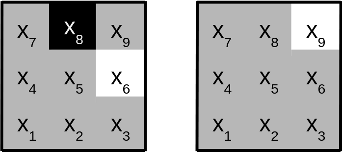
Figure 1: Graphical representation of the logical formula $P^{(1)}_{\mbox{conv}}(x)\lor P_{\mbox{conv}}^{(2)}(x)$, where $P_{\mbox{conv}}^{(1)}(x):=\{(x_{1},\ldots,x_{m})|x_{6}\land\neg x_{8}\mbox{ is true}\}$ and $P_{\mbox{conv}}^{(2)}:=\{(x_{1},\ldots,x_{m})|x_{9}\mbox{ is true}\}$. The first convolutional predicate is displayed on the left side, the second one on the right side. Variables which have to be true in order for the predicate to evaluate to true are marked white. Variables which have to be false in order for the predicate to evaluate to true are marked black. Variables that have no influence on the evaluation are marked gray.

3.2 Stochastic Local Search (SLS)

We implemented the SLS rule learner and extended it for the purpose of pedagogical rule extraction (Algorithm 3). Since we apply SLS to predictive tasks, we adjust SLS to return the candidate that achieved the lowest score on the validation set (line 8). Scores used for the decision rule are still calculated on the training set. Calculation of scores is computationally expensive and SLS needs to evaluate the decision rule in every iteration. Therefore, we calculate scores batchwise. We introduce an adaptation that is theoretically motivated. One can always correct a term that falsely covers an instance by adding one literal, but the same does not hold in the case of an uncovered instance. We account for this by adjusting SLS to remove all literals in a term that differ from an instance (line 22).

Any SLS algorithm starts by evaluating a random solution candidate. It then selects the next candidate from a neighborhood of the former candidate. This procedure is repeated until a solution is found. If no solution is found and no improvement is found for 600 steps, we restart the search with a different random formula. Therefore, one has to define a candidate space, a scoring function to evaluate a candidate solution, a neighborhood of a candidate solution, as well as a decision rule for selecting the next candidate out of a neighborhood. In SLS, the candidate space consists of all applicable k-term DNFs. The scoring function is defined as the number of misclassified instances by a given k-term DNF. The neighborhood of a candidate is given by all k-term DNFs that differ in one literal to the candidate. The next candidate is selected in accordance with a randomly drawn misclassified training instance (line 12). If the instance has a positive training label, with probability $p_{g1}$ a random term is modified (line 14), otherwise the term which differs least from the misclassified instance. With the probability $p_{g2}$ the modification is done by deleting a random literal (line 20). In the case of a negative training label (line 25), any term that covers the considered instance is chosen. In contrast to before, a literal not in accordance with the misclassified instance is added with a probability of $p_{s}$. Otherwise, a literal whose addition decreases the score over the training set most is appended. In the end, SLS returns the candidate that achieves the lowest score on the training set.

1:procedure SLSearch($k,maxIteration,p_{g1},p_{g2},p_{s},batchSize,trainingStop,validationSet$)

2:    $formula$ $\leftarrow$ a randomly generated $k$-term DNF formula

3:    $optimalFormula\leftarrow formula$

4:    $iteration\leftarrow 0$

5:    $minScore\leftarrow\infty$

6:    while  $iteration<maxIteration$ and $minScore>0$ do

7:         $iteration\leftarrow iteration+1$

8:         $newScore\leftarrow score(validationSet)$

9:         if $newScore<minScore$ then

10:             $minScore\leftarrow newScore$

11:             $optimalFormula\leftarrow formula$          

12:         $missedInstance\leftarrow$ random misclassified instance

13:         if $missedInstance$ has positive label then

14:             with probability $p_{g1}$

15:                   $term\leftarrow$ a term uniformly drawn from $formula$

16:             otherwise

17:                   $term\leftarrow$ the term in $formula$ that differs in the smallest

18:                        number of literals from $missedInstance$

19:             with probability $p_{g2}$

20:                   $literals\leftarrow$ a literal uniformly drawn from $term$

21:             otherwise

22:                   $literals\leftarrow$ all literals in $term$ that differ from

23:                        $missedInstance$

24:             $formula\leftarrow formula$ with $literals$ removed from $term$

25:         else if $missedInstance$ has negative label then

26:             $term\leftarrow$ a term in $formula$ that covers $missedInstance$

27:             with probability $p_{s}$

28:                   $literal\leftarrow$ a literal uniformly drawn from all possibilities

29:             otherwise

30:                   $batch\leftarrow$ uniformly pick $batchSize$ many training instances

31:                   $literal\leftarrow$ a literal whose addition to $term$ reduces

32:                        $score(batch)$ the most

33:             $formula\leftarrow formula$ with $literal$ added to $term$              return $optimalFormula$

Algorithm 3:

4 Experimental Evaluation

The code for the following tests can be found on github. The parameters $p_{g1}$, $p_{g2}$ and $p_{s}$ are set to 0.5 for maximal randomness. We perform one-against-all testing so that the ground-truth-labels, which encode the classes of the data as one-hot vectors, are mapped to two classes. One class contains all images with the searched label, the other class contains all other labels. To prevent the neural network from predicting only the majority label, we balanced the labels in the training and test datasets such that one class comprises half of the dataset and the rest of the classes are randomly sampled so that each class is equally represented. We use three commonly used datasets with their predefined train-test splits: MNIST, FASHION-MNIST, and CIFAR10. For each dataset we used 5,000 samples as a holdout set for early stopping of the network and the rest for training. Each dataset has a designated test set with 10,000 samples.

4.1 DCDL – Similarity

In this section we compare our DCDL approach against the black-box SLS algorithm. We look at their ability to model the behavior of a multilayer neural network for the datasets MNIST, FASHION-MNIST and CIFAR10. An overview of the experimental setup is given in Figure 2.

First a neural network is trained, which consists of two convolutional layers followed by a max pooling layer and a sign layer. The last layer is a dense layer with dropout. As soon as the neural net is trained, the output of the sign layers is used as a label for the training of DCDL. The sign layers transform the outputs to binary values for the SLS algorithm. The two convolutional layers and the dense layer are each approximated with Boolean formulas, which are generated by the SLS algorithm. The dithered images are initially used as input to the SLS. After the first SLS, the input in the following SLS runs is the output of the previous formula. The intermediate results of the NN serve as labels.

The approximation of the convolutional operation is, in contrast to the dense layer, not straightforward, so we will explain this process in detail here. Figure 3 shows the process graphically. In a convolutional layer, the input images are subsampled, and the samples are processed with the learned filters. Each sample is mapped to a value. This mapping creates a new representation of the images. Each filter gives its own representation. They are stacked as different channels. With the help of the sign layer, the representations are mapped to binary values.

The process of subsampling also takes place for the input of the DCDL approach. These samples are the input for the SLS algorithm. As labels serves the channel output of the sign layer belonging to the filter which is being approximated with the help of the SLS. Thus, each filter will be approximated by a logical formula. Using this procedure, DCDL approximates the operation of the NN with Boolean formulas.

In the black-box SLS approach, only the input images and the corresponding label predicted by the NN are provided to the algorithm. The architecture of the NN and its functionality are not taken into account. It is evaluated using two different methods. In the black-box prediction approach, the prediction of the neural network is used as a label for training. In the true label approach, the true labels of the images are used for training.

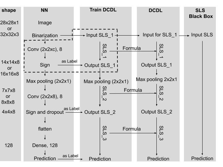
Figure 2: Experimental setup for comparing the neural network, the DCDL and the black-box SLS approach. $c$ depends on the dataset and is the number of color channels. The content of the dotted box is shown in more detail in Figure 3.

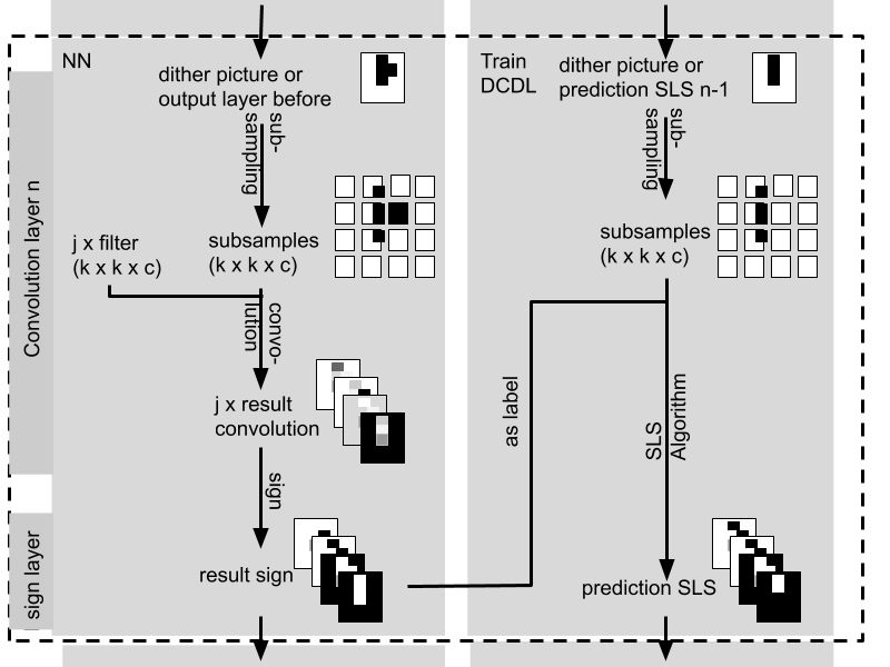
Figure 3: This figure illustrates the approximation of a convolutional layer by the SLS algorithm. It is part of the whole experimental setup in Figure 2 as shown by the dotted box.

We first focus on the question whether DCDL can better approximate the prediction of the neural network than the black-box approaches. Our results in Figure 4 show that DCDL outperforms the black-box approach on the MNIST and Fashion-MNIST dataset and still provide a slight advantage on the CIFAR dataset. We hypothesize that the performance of the neural network itself has an influence on the ability of DCDL to extract good rules. CIFAR is a more complex dataset, and the neural network performs worse than on MNIST. This makes it also more difficult for DCDL to consistently model the network’s behavior.

To calculate the similarity of the labels predicted by the neural network with the labels predicted by the SLS algorithm, we calculate

$$sim=\frac{\sum_{i=1}^{n}\mathbbm{1}[y^{\prime}_{i}=y^{\prime\prime}_{i}]}{n}$$ (5)

with $n$ as the number of labels, $\mathbbm{1}$ the indicator function, $y^{\prime}_{i}$ as the prediction of the investigated approach, and $y^{\prime\prime}_{i}$ as the label calculated by the neural network.

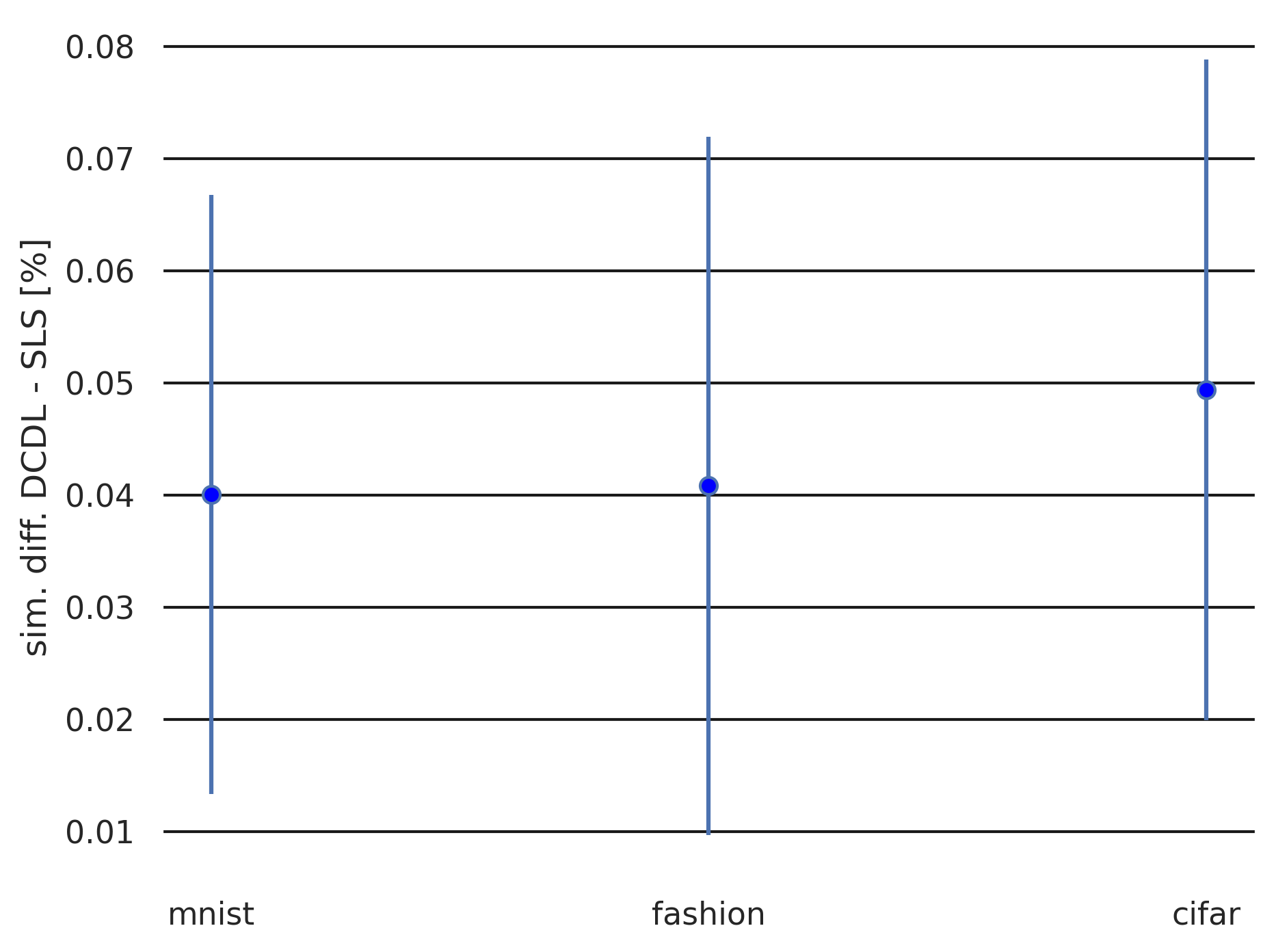
Figure 4: Difference in similarity between the prediction of the DCDL and the black-box approach for $k=40$. The similarity is calculated with respect to the prediction of the neural network on the test set. The DCDL approach has higher similarity across all three datasets. The standard deviation is calculated from 30 runs overall, 3 for each class.

4.2 DCDL – Accuracy

The above section shows that our method performs well in terms of similarity with the neural network. However, clearly, similarity does not necessarily correlate with accuracy. For example, it would be possible that the rule learner only models the errors that the network makes, leading to a high similarity but a bad performance on the actual labels. Therefore, we also compare the accuracy on the true labels of the predictions for the methods DCDL, black-box SLS, and the neural network. For the black-box SLS algorithm, we differentiate between the method that was trained on the labels as predicted by the NN (BB prediction) and the method that was trained on the true labels (BB label). Again we use Equation 5 to calculate the accuracy, but use the true labels of the test data instead of the labels predicted by the neural network.

Our results in Figure 5 show that the neural network outperforms the other methods. DCDL clearly outperforms the black-box approach on the MNIST and Fashion-MNIST datasets and still provides a slight advantage on the CIFAR dataset. The poor performance of the classifiers on the CIFAR dataset is most likely partly caused by the dithering. The network architecture might also play a role. This will be investigated further in our future work.

As shown in Table 1, we also evaluated the statistical significance using a corrected resampled t-test (Nadeau and Bengio, 2003) with $\alpha=0.05$ of the results to show that the performance of DCDL is similar to that of the neural network. For the MNIST and Fashion MNIST datasets, the neural network is not significantly better than DCDL, whereas the black box approach is significantly worse than the neural network. For CIFAR, all rule learning approaches perform worse than the neural network. The reason for this lies in the relative complexity of the dataset. We hypothesize that the network itself is not able to learn a good representation for the dataset, which in turn makes the task for the rule learners harder.

Table 1: p-values of the corrected resampled t-test (Nadeau and Bengio, 2003) for MNIST, FASHION-MNIST and CIFAR for the accuracy values shown in Figure 5. Gray-shaded are the pairs for which the null hypothesis is rejected with significance level $\alpha=0.05$ using a corrected resampled t-test (Nadeau and Bengio, 2003).

	BB prediction	BB label	Neural network
MNIST
DCDL	0.59	0.27	0.00
BB prediction	-	0.07	0.00
BB label	-	-	0.02
Fashion
DCDL	0.03	0.10	0.00
BB prediction	-	0.81	0.00
BB label	-	-	0.01
Cifar
DCDL	0.08	0.04	0.00
BB prediction	-	0.90	0.00
BB label	-	-	0.00

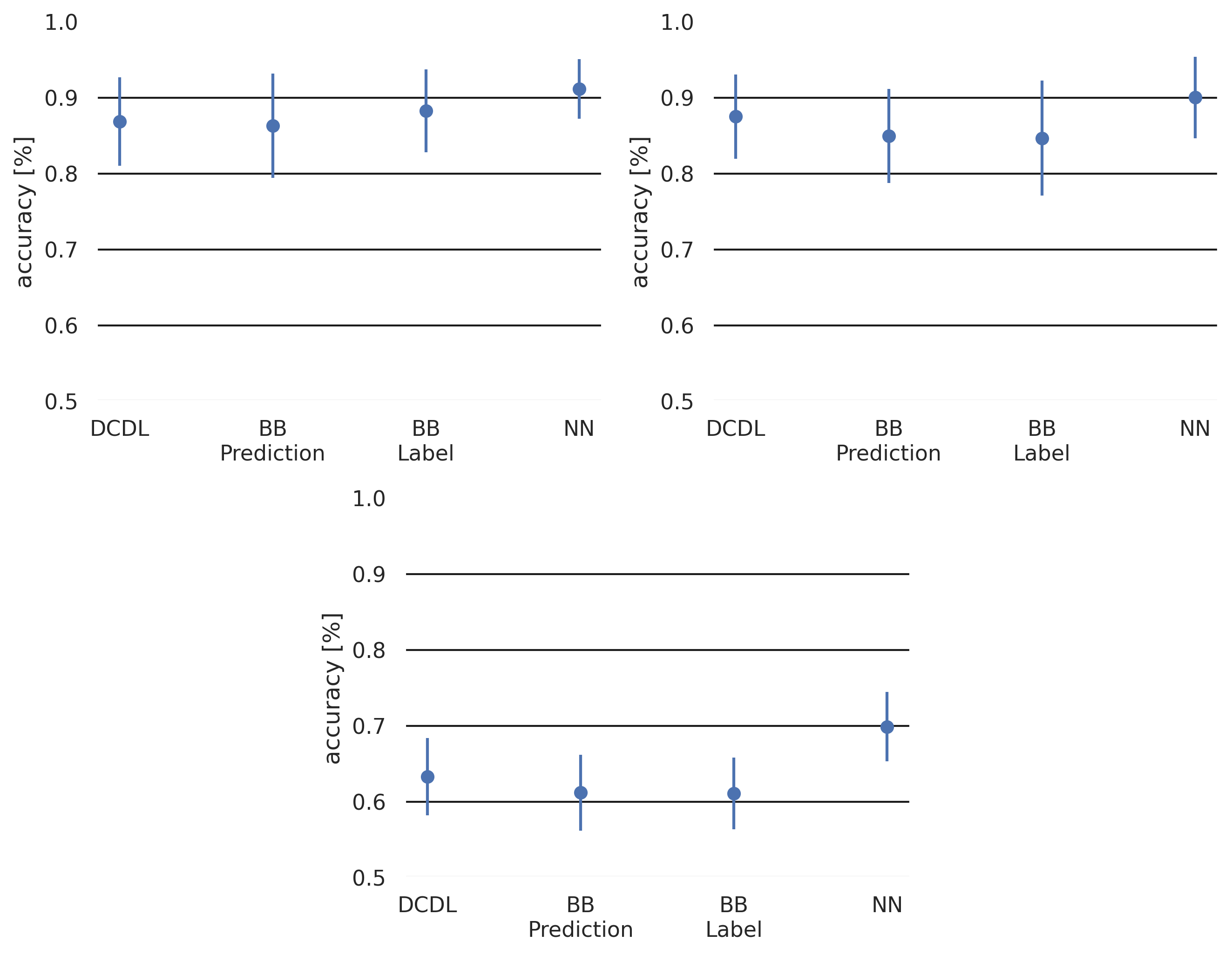
Figure 5: Accuracy for different datasets of our DCDL approach, the black-box SLS, black-box SLS with true labels, and the neural network. Top left: MNIST, top right: FASHION-MNIST, bottom: CIFAR. For SLS we used $k=40$. The standard deviation is calculated from 30 runs overall, 3 for each class.

4.3 Visualization of logical formulas

We already showed an example for the visualization of a simple formula in Section 3.1.1. Now, we want to look at the visualization of more complex formulas that are found by our algorithm. If the rule search is conducted with a small $k$, the visualized rules tend to be discriminative and often highlight only a single pixel, thus making them hard to interpret. To counter this, we set $k$ to higher values in order to learn rules that are more characteristic. However, when visualizing $k$ predicates for high $k$, this produces a lot of images. Therefore, we add a reduce step that sums and renormalizes the visualizations for all $k$ predicates. As Figure 6 shows, this leads to clear visualizations that look almost like probability densities or prototypes. The comparison to the convolutional filters shows that this procedure leads to visualizations that are more easily identifiable by the human eye.

The architecture of the neural network is shown in Figure 7. It consists of a convolutional layer followed by a sign layer and a dense layer. The dense layer converts the scalar output of the sign layer into a one-hot vector. The weights of the dense layer were set to [1,0]. The dithered images are the input for the SLS algorithm and the output of the sign layer is the label for the SLS algorithm. The visualization in Figure 6 was done on the MNIST dataset with a filter size that is equal to the size of the image. Note that for the case of MNIST, smaller filter sizes do not result in interpretable visualizations. However, in principle we can also choose filter sizes much smaller than the image itself if the images consist of complex scenes where the number itself is only a small part of the image for example. The selection of a filter size that leads to an interpretable visualization is left for future work. To sum up, we showed with the help of a simple example how the individual predicates as well as the complete convolutional rule may be visualized.

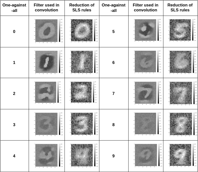
Figure 6: Results of visualizing convolutional rules rules with $k=150$. The convolutional filter by the NN is shown for comparison.

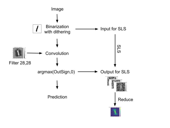
Figure 7: Test setup for approximating convolution operations with logical formulas.

5 Conclusion

We investigated how convolutional rules enable the extraction of interpretable rules from binary neural networks. We showed the successful visualization by means of an example. Additionally, the similarity to the functionality of the neural network was measured on three different datasets and found to be higher for the decompositional approach than the black-box approach. We think there is potential in decompositional approaches for the extraction and visualization of characteristic rules. Although the logical formulas are large for human visual inspection on real-world data, their representation makes deep learning models, in principle, amenable to formal verification and validation.

In future research, we aim to incorporate further state-of-the-art components of NNs while preserving the ability of the network to be transformed into (convolutional) logical rules. Our work suggests that the combination of binary NNs and k-DNF is promising combination. To this end, one should develop a differentiable version of DCDL based on, e.g., differentiable sub modular maximization (Tschiatschek et al., 2018) or differentiable circuit SAT (Powers et al., 2018). Generally, one should explore DCDL as a new prespective on neuro-symblic AI (Garcez and Lamb, 2020).

Permission to Reuse and Copyright

Figures, tables, and images will be published under a Creative Commons CC-BY licence, and permission must be obtained for use of copyrighted material from other sources (including re-published/adapted/modified/partial figures and images from the internet). It is the responsibility of the authors to acquire the licenses, to follow any citation instructions requested by third-party rights holders, and cover any supplementary charges.

Conflict of Interest Statement

The authors declare that the research was conducted in the absence of any commercial or financial relationships that could be construed as a potential conflict of interest.

Author Contributions

The experiments were done by JB. The initial code basis was due to NW, the writing of the paper was mainly done by SB with input from JB and NW. ZA and SK were involved in the development of ideas, the polishing of the paper, and discussions throughout. KK gave feedback to the paper and helped with the writing of the submitted manuscript.

Funding

The work was funded by the RMU Initiative Funding for Research by the Rhine Main universities (Johannes Gutenberg University Mainz, Goethe University Frankfurt and TU Darmstadt) within the project “RMU Network for Deep Continuous-Discrete Machine Learning (DeCoDeML)”.

References

- Andrews et al. (1995) Robert Andrews, Joachim Diederich, and Alan B. Tickle. Survey and critique of techniques for extracting rules from trained artificial neural networks. Knowledge-Based Systems, 8(6):373 – 389, 1995. Knowledge-based neural networks.
- Augasta and Kathirvalavakumar (2011) M. Gethsiyal Augasta and T. Kathirvalavakumar. Reverse engineering the neural networks for rule extraction in classification problems. Neural Processing Letters, 35:131–150, 2011.
- Bengio et al. (2013) Yoshua Bengio, Nicholas Léonard, and Aaron C. Courville. Estimating or propagating gradients through stochastic neurons for conditional computation. CoRR, abs/1308.3432, 2013.
- Craven and Shavlik (1995) Mark W. Craven and Jude W. Shavlik. Extracting tree-structured representations of trained networks. In Proceedings of the 8th International Conference on Neural Information Processing Systems, NIPS’95, page 24–30, Cambridge, MA, USA, 1995. MIT Press.
- Fu (1994) LiMin Fu. Rule generation from neural networks. IEEE Transactions on Systems, Man, and Cybernetics, 24(8):1114–1124, 1994.
- Garcez and Lamb (2020) Artur d’Avila Garcez and Luis C Lamb. Neurosymbolic ai: The 3rd wave. arXiv preprint arXiv:2012.05876, 2020.
- Gehring et al. (2017) Jonas Gehring, Michael Auli, David Grangier, Denis Yarats, and Yann N. Dauphin. Convolutional sequence to sequence learning. In Proceedings of the 34th International Conference on Machine Learning, ICML 2017, Sydney, NSW, Australia, 6-11 August 2017, pages 1243–1252, 2017.
- González et al. (2017) Camila González, Eneldo Loza Mencía, and Johannes Fürnkranz. Re-training deep neural networks to facilitate boolean concept extraction. In International Conference on Discovery Science, pages 127–143. Springer, 2017.
- Hinton (2012) Geoffrey Hinton. Neural networks for machine learning. Coursera Video Lectures, 2012.
- Hinton et al. (2015) Geoffrey E. Hinton, Oriol Vinyals, and Jeffrey Dean. Distilling the knowledge in a neural network. CoRR, abs/1503.02531, 2015.
- Hu et al. (2016) Zhiting Hu, Xuezhe Ma, Zhengzhong Liu, Eduard Hovy, and Eric Xing. Harnessing deep neural networks with logic rules. arXiv preprint arXiv:1603.06318, 2016.
- Hubara et al. (2016) Itay Hubara, Matthieu Courbariaux, Daniel Soudry, Ran El-Yaniv, and Yoshua Bengio. Binarized neural networks. In D. D. Lee, M. Sugiyama, U. V. Luxburg, I. Guyon, and R. Garnett, editors, Advances in Neural Information Processing Systems 29, pages 4107–4115. Curran Associates, Inc., 2016.
- Huth and Ryan (2004) Michael Huth and Mark Ryan. Logic in Computer Science: Modelling and Reasoning about Systems. Cambridge University Press, USA, 2004. ISBN 052154310X.
- Kane and Milgram (1993) Raqui Kane and Maurice Milgram. Extraction of semantic rules from trained multilayer neural networks. In IEEE International Conference on Neural Networks, pages 1397–1401. IEEE, 1993.
- Lin et al. (2017) Xiaofan Lin, Cong Zhao, and Wei Pan. Towards accurate binary convolutional neural network. In Advances in Neural Information Processing Systems, pages 345–353, 2017.
- Liu et al. (2018) Zechun Liu, Baoyuan Wu, Wenhan Luo, Xin Yang, Wei Liu, and Kwang-Ting Cheng. Bi-real net: Enhancing the performance of 1-bit cnns with improved representational capability and advanced training algorithm. In The European Conference on Computer Vision (ECCV), pages 747–763, September 2018.
- Mahendran and Vedaldi (2015) Aravindh Mahendran and Andrea Vedaldi. Understanding deep image representations by inverting them. In Proceedings of the IEEE conference on computer vision and pattern recognition, pages 5188–5196, 2015.
- Mnih et al. (2013) Volodymyr Mnih, Koray Kavukcuoglu, David Silver, Alex Graves, Ioannis Antonoglou, Daan Wierstra, and Martin A. Riedmiller. Playing atari with deep reinforcement learning. CoRR, abs/1312.5602, 2013.
- Nadeau and Bengio (2003) Claude Nadeau and Yoshua Bengio. Inference for the generalization error. Machine learning, 52(3):239–281, 2003.
- Odense and Garcez (2020) Simon Odense and Artur Garcez. Layerwise knowledge extraction from deep convolutional networks. In NeurIPS 2019 Workshop on Knowledge Representation & Reasoning Meets Machine Learning, 2020.
- Poplin et al. (2018) Ryan Poplin, Pi-Chuan Chang, David Alexander, Scott Schwartz, Thomas Colthurst, Alexander Ku, Dan Newburger, Jojo Dijamco, Nam Nguyen, Pegah T. Afshar, Sam S. Gross, Lizzie Dorfman, Cory Y. McLean, and Mark A. DePristo. Creating a universal snp and small indel variant caller with deep neural networks. bioRxiv, 2018.
- Powers et al. (2018) Thomas Powers, Rasool Fakoor, Siamak Shakeri, Abhinav Sethy, Amanjit Kainth, Abdel-rahman Mohamed, and Ruhi Sarikaya. Differentiable greedy networks. arXiv preprint arXiv:1810.12464, 2018.
- Quinlan (2014) J Ross Quinlan. C4. 5: programs for machine learning. Elsevier, 2014.
- Rastegari et al. (2016) Mohammad Rastegari, Vicente Ordonez, Joseph Redmon, and Ali Farhadi. Xnor-net: Imagenet classification using binary convolutional neural networks. In European conference on computer vision, pages 525–542. Springer, 2016.
- Ribeiro et al. (2016) Marco Tulio Ribeiro, Sameer Singh, and Carlos Guestrin. “why should i trust you?”: Explaining the predictions of any classifier. In Proceedings of the 22nd ACM SIGKDD International Conference on Knowledge Discovery and Data Mining, KDD ’16, page 1135–1144, New York, NY, USA, 2016. Association for Computing Machinery. ISBN 9781450342322.
- Ross et al. (2017) Andrew Slavin Ross, Michael C. Hughes, and Finale Doshi-Velez. Right for the right reasons: Training differentiable models by constraining their explanations. In Proceedings of the Twenty-Sixth International Joint Conference on Artificial Intelligence, IJCAI-17, pages 2662–2670, 2017. doi: 10.24963/ijcai.2017/371. URL https://doi.org/10.24963/ijcai.2017/371.
- Rückert and Kramer (2003) Ulrich Rückert and Stefan Kramer. Stochastic local search in k-term DNF learning. In Machine Learning, Proceedings of the Twentieth International Conference (ICML 2003), August 21-24, 2003, Washington, DC, USA, pages 648–655, 2003.
- Schmitz et al. (1999) Gregor PJ Schmitz, Chris Aldrich, and Francois S Gouws. Ann-dt: an algorithm for extraction of decision trees from artificial neural networks. IEEE Transactions on Neural Networks, 10(6):1392–1401, 1999.
- Sethi et al. (2012) K. K. Sethi, D. K. Mishra, and B. Mishra. Kdruleex: A novel approach for enhancing user comprehensibility using rule extraction. In 2012 Third International Conference on Intelligent Systems Modelling and Simulation, pages 55–60, 2012.
- Setiono and Leow (2000) Rudy Setiono and Wee Kheng Leow. Fernn: An algorithm for fast extraction of rules fromneural networks. Applied Intelligence, 12(1–2):15–25, January 2000. ISSN 0924-669X. doi: 10.1023/A:1008307919726. URL https://doi.org/10.1023/A:1008307919726.
- Simonyan et al. (2013) Karen Simonyan, Andrea Vedaldi, and Andrew Zisserman. Deep inside convolutional networks: Visualising image classification models and saliency maps. arXiv preprint arXiv:1312.6034, 2013.
- Stecher et al. (2016) Julius Stecher, Frederik Janssen, and Johannes Fürnkranz. Shorter rules are better, aren’t they? In Toon Calders, Michelangelo Ceci, and Donato Malerba, editors, Discovery Science, pages 279–294, Cham, 2016. Springer International Publishing.
- Stone et al. (2017) Austin Stone, Huayan Wang, Michael Stark, Yi Liu, D Scott Phoenix, and Dileep George. Teaching compositionality to cnns. In Proceedings of the IEEE Conference on Computer Vision and Pattern Recognition, pages 5058–5067, 2017.
- Taha and Ghosh (1999) Ismail A Taha and Joydeep Ghosh. Symbolic interpretation of artificial neural networks. IEEE Transactions on knowledge and data engineering, 11(3):448–463, 1999.
- Thrun (1995) Sebastian Thrun. Extracting rules from artificial neural networks with distributed representations. In Advances in neural information processing systems, pages 505–512, 1995.
- Thrun (1993) Sebastian B. Thrun. Extracting provably correct rules from artificial neural networks. Technical report, University of Bonn, 1993.
- Tschiatschek et al. (2018) Sebastian Tschiatschek, Aytunc Sahin, and Andreas Krause. Differentiable submodular maximization. In Proceedings of the Twenty-Seventh International Joint Conference on Artificial Intelligence, IJCAI-18, pages 2731–2738. International Joint Conferences on Artificial Intelligence Organization, 7 2018. doi: 10.24963/ijcai.2018/379. URL https://doi.org/10.24963/ijcai.2018/379.
- Tsukimoto (2000) Hiroshi Tsukimoto. Extracting rules from trained neural networks. IEEE Transactions on Neural networks, 11(2):377–389, 2000.
- Zeiler and Fergus (2014) Matthew D Zeiler and Rob Fergus. Visualizing and understanding convolutional networks. In European conference on computer vision, pages 818–833. Springer, 2014.
- Zhang et al. (2018) Quanshi Zhang, Ying Nian Wu, and Song-Chun Zhu. Interpretable convolutional neural networks. In Proceedings of the IEEE Conference on Computer Vision and Pattern Recognition, pages 8827–8836, 2018.
- Zhou et al. (2016) Bolei Zhou, Aditya Khosla, Agata Lapedriza, Aude Oliva, and Antonio Torralba. Learning deep features for discriminative localization. In Proceedings of the IEEE conference on computer vision and pattern recognition, pages 2921–2929, 2016.
- Zilke et al. (2016) Jan Ruben Zilke, Eneldo Loza Mencía, and Frederik Janssen. Deepred - rule extraction from deep neural networks. In International Conference on Discovery Science, pages 457–473, 2016.