Scaling pair count to next galaxy surveys

Abstract

Counting pairs of galaxies or stars according to their distance is at the core of real-space correlation analyzes performed in astrophysics and cosmology. Upcoming galaxy surveys (LSST, Euclid) will measure properties of billions of galaxies challenging our ability to perform such counting in a minute-scale time relevant for the usage of simulations. The problem is only limited by efficient access to the data, hence belongs to the big data category. We use the popular Apache Spark framework to address it and design an efficient high-throughput algorithm to deal with hundreds of millions to billions of input data. To optimize it, we revisit the question of nonhierarchical sphere pixelization based on cube symmetries and develop a new one dubbed the "Similar Radius Sphere Pixelization" (SARSPix) with very close to square pixels. It provides the most adapted indexing over the sphere for all distance-related computations. Using LSST-like fast simulations, we compute autocorrelation functions on tomographic bins containing between a hundred million to one billion data points. In each case we achieve the construction of a standard pair-distance histogram in about 2 minutes, using a simple algorithm that is shown to scale, over a moderate number of nodes (16 to 64). This illustrates the potential of this new techniques in the field of astronomy where data access is becoming the main bottleneck. They can be easily adapted to other use-cases as nearest-neighbors search, catalog cross-match or cluster finding. The software is publicly available from https://github.com/astrolabsoftware/SparkCorr.

1 Introduction

Since the very beginning of large-scale structure studies (Peebles, 1980), counting the number of pairs of galaxies according to their distance is the basis for the estimation of two-point correlation functions in cosmology. Including also today the measured ellipticities to infer the cosmic shear provides invaluable information on the dark energy at an epoch it starts playing a sizable role on structure formation. The statistically most powerful way to analyze the data is through the so-called “$3\times 2$-points” method, which combines two galaxy samples, a faint one with estimated shear distortions and a smaller one with more stringent selection criteria (e.g., Kilbinger, 2015). One then performs both autocorrelations and cross-correlation between the shears and the positions which allows not only to estimate cosmological and nuisance parameters but also to carry out systematic tests. (e.g., Mandelbaum, 2018). There are in fact more than three correlation functions since the galaxy population is split into redshift bins (the tomographic shells) and correlations are performed between them which allows a model independent data analysis still with negligible precision loss for photometric surveys.

The latest tomographics surveys (Abbott et al., 2018; Hikage et al., 2019; Asgari et al., 2020) use shells with tens of millions of objects (for the faint sample). State-of-the-art algorithms, treecorr (Jarvis et al., 2004) or CUTE (Alonso, 2013) are run to compute the shear-shear, position-position and shear-position statistics. These algorithms are based on High Performance Computing (HPC) on supercomputers and results are obtained within minutes on those $\mathcal{O}(10^{7})$ datasets.

The next generation of galactic surveys, the ground-based Vera C. Rubin Observatory Legacy Survey of Space and Time (LSST) (LSST Science Collaboration et al., 2009) and Euclid spatial mission (Laureijs et al., 2011) will push the statistics much higher, measuring properties of billions of galaxies. The planned tomographic shells will then contain hundreds of millions of objects. To our knowledge no pair-counting algorithm can attain minutes performances with such numbers.

Distance binned pair-counting is not a CPU intensive computation. It is only limited by heavy combinatorics, i.e. by efficient access to the data. It becomes then natural to inspect if “big data” methods can be of any help here. A popular tool to analyze huge amounts of data is Apache Spark (Zaharia et al., 2012, 2010) which is an efficient implementation of the original map-reduce paradigms presented by Google (e.g., Dean & Ghemawat, 2008) and of several tools developed in the Hadoop ecosystem . We point out that this branch of computing, loosely known as High Throughput Computing (HTC) relies on ideas that are very different from the standard operative methods (e.g. in fortran, C++), using for instance the functional programming paradigm that is getting popular these years due to excellent performances over large datasets.

Spark is essentially used by private companies although some dedicated systems using it were also successfully developed in astrophysics for instance to organize data access (Zečević et al., 2018; Brahem et al., 2018b). It is a multi-purpose engine that can deal not only with standard multi-variable analysis with the SQL module (Armbrust et al., 2015), but also with large graphs (with some application to astrophysics in (Hong et al., 2020)), machine learning (Meng et al., 2015) and streaming capabilities (with a recent applications to an alert broker in Möller et al. (2020)).

Although not much used in science, the goal of this work is to show that a tool like Spark can address some modern limitations due to heavy data access and will become more and more pertinent in the next years. Furthermore as will be shown, we try to convince users that beside changing some habits, the learning curve is quite smooth and rapid. With little work one can obtain the same performances than dedicated software developed by experts for years.

In the following we will use only some very basic aspects of Spark, namely dataframes much popularized in astrophysics by the python pandas package. A pedagogical introduction to the use of Spark dataframes in cosmology and astrophysics is given in Plaszczynski et al. (2019) (see also references therein for more applications to astrophysics) but we will still review some basics at the beginning of Sect. 2. Then, we will give the main ideas on how to reduce the pair-counting combinatorics. They are not new, but we show how they can be adapted to Spark.

To improve on performances, we will the revisit the question of sphere indexing in Sect. 3 and propose an adapted new pixelization scheme. Although it was initially designed to improve on our pair-counting algorithm, its scope is much more general. It can be used to pad the sphere with similar shape quadrangles and is thus the best candidate for all distance-related computations. This section is essentially independent from the others.

Then we present in Sect. 4 the results obtained with a logarithmic binning used by the DES Collaboration, on $10^{8}$ to $10^{9}$ data points and detail performances before concluding on the overall interest of the method. A gives some more information on some cubed-base pixelization properties.

2 Pair counting with Apache Spark

2.1 Introduction to Spark SQL

Spark is a framework to work efficiently on a cluster of machines not necessarily designed with (expensive) high speed connections, what is loosely called a data-center. It is based on a driver-executor architecture: one machine (the driver) sends instructions to a set of workers (executors), that perform some tasks and send back some (reduced) results that are then combined by the driver. One could say that the big data approach is about "sending computation to the data" while HPC does it the reverse way, move the data to the compute units. The essential feature here is then how data are stored and also preserved through multiple copies, on each worker. This is called data partionning: the goal is to achieve some locality to avoid inter-nodes communications and it depends on the problem being studied. Here for instance we will partition our dataset according to some pixel number meaning gathering points (galaxies) within the same region of the sky on the same workers. Beyond partitioning, an essential feature of Spark is the ability to put the data in the executors’ Random Access Memory hereafter, the cache. This boosts performances considerably and for the user it is equivalent to having a single “ machine” with hundreds of Gigabytes of memory. While the implementation under the hood can be quite complex, on the user side it is not more complicated than calling the partition() or cache() dataframe methods.

Spark is a full framework with many functionalities, but we will be concerned here only with dataframes which are part of the so-called Spark SQL module. Dataframes are not specific to Spark nor even coming from the big-data field (one can find similar ideas since the 70’s in High Energy Physics where they are called "n-tuples"). What Spark does is implement efficiently some standard operations on them in a distributed environment.

A dataframe can be thought of simply as a table of values (a dataset of rows), with some named columns. In our case the columns are 2 angles on the sky ("RA" and “DEC") and some identifier ("id", a long integer).

It is read from a file either in FITS format (using the spark-fits connector, Peloton et al. (2018)), either natively as plain text or in parquet format, the latter being the choice we made. We will call this dataframe the source. Let us now review some important operations with dataframes that we will use.

The most obvious one is to filter the dataframe meaning applying conditions depending on some column values (as applying cuts) to obtain a reduced one.

Another important operation is the groupBy. For a given dataframe one can group rows according to some criteria and perform some further operation of the grouped array to end up with some value (as the number of its elements). To illustrate it let us see how to obtain a histogram for some column as for instance the “RA” angle. First one adds a new column with the bin number corresponding to each RA value. Then one groupBy this bin number and count the number of elements to estimate the frequency within each bin. Here is how it would look like with Spark in python:

⬇

# NB: files are available online

# see "data availability" section

src=spark.read.parquet("tomo100M.parquet")

# what’s in it?

src.show(3)

+---------+----------+

| RA| DEC|

+---------+----------+

|180.77408|-40.784428|

|180.78752| -40.85317|

|180.75848|-40.799908|

+---------+----------+

# let us do a histogram on "RA" (10 degrees bins)

# 1. add the bin number

h=src.withColumn("bin",(df.RA/10).astype(’int’))

# check

h.show(3)

+---------+----------+---+

| RA| DEC|bin|

+---------+----------+---+

|180.77408|-40.784428| 18|

|180.78752| -40.85317| 18|

|180.75848|-40.799908| 18|

+---------+----------+---+

# 2. bin counting: groupby bin number

# and count the number of elements in each group

h=h.groupBy("bin").count()

# check

h.show(3)

+---+-----+

|bin|count|

+---+-----+

| 26|61288|

| 12|60965|

| 22|89625|

+---+-----+

# then we may sort according to the bin number,

# add bin centers etc.

With two dataframes, one can perform a join operation: this means creating a dataframe where each row is obtained by “gluing” together two rows from the previous ones, according to a common column value. For instance let us add to each row of the source some pixel number. If we perform a join operation between the source and itself based on the pixel number, we will end up with a dataframe containing all pairs having the same pixel number. We always use some inner- join operations which means that the two rows must exist in each dataframe to perform the gluing. To remove auto-pairs and reverse-id pairs we filter the output requiring that the first id be lower than the second. An example of such operation is show in Table 1.

RA	DEC	id	ipix
180.77	-40.78	0	0
180.79	-40.85	1	0
180.76	-40.80	2	0
180.65	-41.00	3	1
180.55	-41.01	4	1
180.46	-40.81	5	1

RA2	DEC2	id2	ipix
180.77	-40.78	0	0
180.79	-40.85	1	0
180.76	-40.80	2	0
180.65	-41.00	3	1
180.55	-41.01	4	1
180.46	-40.81	5	1

inner-join
$\big{\Downarrow}$
ipix RA DEC id RA2 DEC2 id2 0 180.77 -40.78 0 180.79 -40.85 1 0 180.77 -40.78 0 180.76 -40.80 2 0 180.79 -40.85 1 180.76 -40.80 2 1 180.65 -41.00 3 180.55 -41.01 4 1 180.65 -41.00 3 180.46 -40.81 5 1 180.55 -41.01 4 180.46 -40.81 5

Table 1: Illustration of the inner-join operation. The upper left table represent the source dataframe with some angular positions (RA/DEC), an identifier (id) and a pixel number ("ipix"). The upper right is just a copy of it with the columns renamed but for "ipix". The lower table is the result of applying an inner-join operation based on "ipix" and filtering the output according to $id<id2$. It contains all the pairs of points with the same pixel value.

This is a very optimized way of building all pairs of nearby points but that neglects the case where each point lies across a pixel boundary (as A and B on Fig.1). To resolve it we will use a trick due to Brahem et al. (2018a). Starting from the source dataframe we do not simply copy it as in Tab.1. Instead each row is replicated and indexed not only by its pixel number but also by its 8 neighboring pixel numbers. We will call this 9 times larger dataframe, the duplicates one. Consider points A and B on Fig.1 with their pixel number. In a symbolic form we can write the source dataframe as : $(A,3),(B,5)$. In the duplicates dataframe the B point is repeated 9 times : $(B,1),(B,2),(B,2),(B,3),(B,4),(B,5),(B,6),(B,7),(B,9)$. Consider what happens in an inner-join between the source and its duplicates: only the $(A,3),(B,3)$ pair has a common index and will be retained in the join operation. In this way we build the pairs between all points lying in the same pixel but also in the neighboring ones. Of course many pairs will have a too large distance now. But once the pair dataframe is available one can compute exactly the distance between them and filter precisely on it.

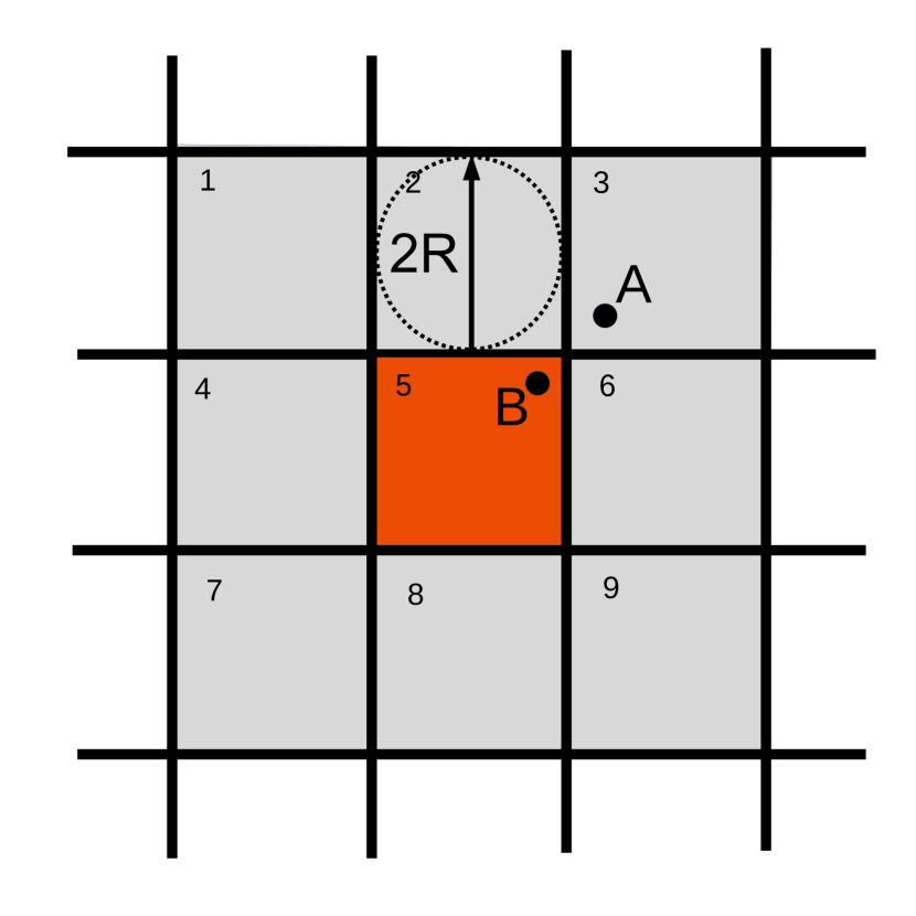
Figure 1: Illustration of pair building on a pixel grid (square lattice here). The grey pixels corresponds to the neighbours of the red one and will be denoted duplicates (including the red one itself). The numbers denote some pixel indices. The radius involved for the choice of the pixel size is shown and corresponds to the inner radius of the pixel.

2.2 Binning

Counting pairs according to the distance between objects in order to compute correlation functions is always performed within a histogram defined by a given binning. As an illustration, we will use later the one used by the DES Collaboration in their first year $3\times 2$ point analysis (Abbott et al., 2018) which consists of 20 bins uniformly spaced on a logarithmic scale from 2.5′to 250′. Results will be discussed in detail in Sect. 4 and we only emphasize here that because of the logarithmic scale the bin width increases with the bin number. We will focus on the autocorrelation of the shear sample which has the most intensive combinatorics. Since computing shear-related quantities is not CPU-limiting we just study hereafter the performance of pair counting.

2.3 Building pairs

Working on more than $\mathcal{O}(10^{8})$ data points, the raw number of pairs scaling as $N^{2}$ precludes any hope for computing all the pair-distances. Fortunately, there exists some classical methods to reduce combinatorics and we show how they can be implemented in Spark.

The fist obvious one is to compute distances only for pairs that are below the upper bin cutoff. To this end we add some pixel index with a suitable size that will be discussed later. Then, as explained in Sect. 2.1 we use an inner-join operation betwen the source and the duplicates dataframes on it.

Let us consider that there are $N_{\mathrm{pix}}^{J}$ pixels over the sphere. Then assuming each pixel holds $\textrm{N}_{\mathrm{data}}/N_{\mathrm{pix}}^{J}$ values in average, the number of pairs reduces to

$$N_{\textrm{pairs}}^{X}\approx N_{\mathrm{pix}}^{J}\times\dfrac{1}{2}\left(\dfrac{\textrm{N}_{\mathrm{data}}}{N_{\mathrm{pix}}^{J}}\right)^{2}=\dfrac{\textrm{N}_{\mathrm{data}}^{2}}{2N_{\mathrm{pix}}^{J}}.$$ (1)

However since we will be considering pixelization with essentially 8 neighbours, the duplicates dataframe is 9 time larger than the input data. Then the combinatorics increases to:

$$N_{\textrm{pairs}}^{X}\approx\dfrac{9^{2}\textrm{N}_{\mathrm{data}}^{2}}{2N_{\mathrm{pix}}^{J}}.$$ (2)

We see that we want the largest possible number of pixels to decrease combinatorics, i.e. the most compact padding of the sphere. This will be the topic of Sect. 3. We will call this pixelization the joining one and since this method calculates exact distances, we refer to it hereafter as the "exact method".

2.4 Reducing the data

Suppose we can group the data into areas on the sky where all the points are below some distance $R$ from their center. A first one has $N_{1}$ elements and the second one $N_{2}$. Calling $d_{c}$ the distance between the two area, the separation between any pair of points can be written as (see Fig.2)

$$r_{ij}=d_{c}+\epsilon$$ (3)

where $\epsilon$ is a random variable satisfying

$$\left\lvert\epsilon\right\rvert<2R.$$ (4)

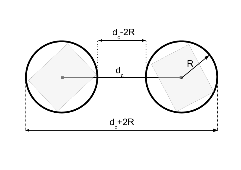
Figure 2: Sketch to illustrate the pixel size involved in data compression. Pixels (gray quadrangles) are contained in their circumscribed circle and their centers are distant by $d_{c}$. The angular distance between any pair of points in each pixel is contained within $[d_{c}-2R,d_{c}+2R]$. The radii involved here are the pixel outer ones.

Let first consider a linear binning starting at $r_{0}$ of width $w$. The bin number is obtained from

$$\left\lfloor\dfrac{r_{ij}-r_{0}}{w}\right\rfloor\simeq\left\lfloor\dfrac{d_{c}-r_{0}}{w}\right\rfloor+\left\lfloor\dfrac{\epsilon}{w}\right\rfloor$$ (5)

$\lfloor\rfloor$ being the floor operator. This is not a strict equality since $\epsilon$ introduces some smearing along the bin borders, but is a reasonable approximation if $\epsilon\ll d_{c}-r_{0}$ and will be tested later (Sect. 4.3.3). Then if $R$ satisfies

$$2R<w$$ (6)

the last term of Eq. (5) is zero. Then, up to a tiny effect across the boundaries, all pairs have their angular separation falling withing the same bin, so their contributions can be immediately computed as $N_{1}N_{2}$.

Concerning the logarithmic binning scheme, as the bin width increases with the angular separation, if we choose for $w$ its very first value, Eq. (6) is automatically satisfied for all the others.

To ensure that all point angular distances lie below a given radius, we use a new pixelization with a pixel size adapted to Eq. (6). We will refer to it in the following as the reducing pixelization.

We replace our input data by a new dataframe consisting of pixels, using their center as position and keeping their number count. This is performed efficiently with a groupBy operation (see Sect. 2.1). We then proceed following Sect. 2.3 changing the binning part by the cumulative count of the product numbers.

When it can be applied, i.e. when first the bin width is large enough that the number of pixels $N_{\mathrm{pix}}^{D}$ is lower than the input data size, it is a very efficient compression scheme since the number of pairs decreases quadratically and Eq. (2) in this case becomes

$$N_{\textrm{pairs}}^{R}\approx\dfrac{9^{2}(N_{\mathrm{pix}}^{D})^{2}}{2N_{\mathrm{pix}}^{J}}.$$ (7)

We will call this method the reduced one.

2.5 Algorithm overview

We have now all in hands to design the pair counting algorithm with Spark. We consider some given binning and first work out the first bins with the exact algorithm. The discussion on the number of bins effectively treated is deferred to a concrete example in Sect. 4. We divide the algorithm into three main parts.

1. Source:

   • : read the input data angular coordinates into the source dataframe, convert to Cartesian ones and add an increasing identifier on al the data.

   • : add a joining pixel index.

   • : do a repartition of the dataframe according to the pixel index and push it to the workers cache.

2. Duplicates:

   • : construct a new dataframe from the source by re-indexing it to all the neighboring pixels.

   • : concatenate source.

   • : do a repartition of the dataframe according to the pixel index and push it to the workers cache.

3. Join:

   • : perform the (inner) join between the source and its duplicates to create all pairs.

   • : filter pairs for which the first identifier is lower than the second one, compute the distances and only keep distances that are below the upper bin cutoff.

   • : assign bin number to each distance and count.

The source part is mainly limited by reading the data from disks (I/O), the duplicates part is more concerned by the network finite bandwidth and the join part by accessing the data and doing actual computations.

The reduced method is applied for the the following bins. It is essentially the same than the previous one but adds a preliminar stage to transform the input data:

1. Reduction:

   • : read and add a new index to the data (reducing pixelization).

   • : group the points according to the R1 index and keep the number count (groupBy+count).

   • : compute and store the centers of the pixels in a new dataframe.

Then we proceed according to the previous 1-3 steps using this dataframe as our data, with a tiny modification to J3 since the bin numbers are now computed from the product of the number of galaxies.

Before illustrating how it performs on a concrete case (Sect. 4) we need to address the question of an adapted spatial space indexing, i.e. revisit the ancient question of sphere pixelization.

3 Best spatial sphere indexing

The indexing of the unit sphere enters in two different places in our method.

1. Joining index (S2) : the indexing scheme allows computing angular distances only for pairs that are below some upper $\theta_{+}$ cut. One needs a pixel size large enough that any pair of points within it is below the largest angular size of the problem. We aim to get the total number of pixels $N_{\mathrm{pix}}^{D}$ to be as large as possible (Eq. (15)).

2. Data reduction index (R1): in this step we replace our data by pixels when their size is smaller than the smallest bin width of the problem. According to Eq. (7) the goal is to choose the total number of pixels $N_{\mathrm{pix}}^{D}$ as low as possible.

As shown on Fig.1, the S2 step concerns the pixel inner radius, defined by the largest inscribed circle, while the R2 step concerns its outer radius (Fig.2) defined by the smallest circumscribing circle. Depending on the tiling, pixels have different shapes so that the inner and outer radii vary accordingly. For a given angular distance scale one must then use the minimal (inner case) or maximal (outer case) values in order to be valid everywhere.

Our factor of merit is then to have a high padding of the sphere leading to a high (resp. low) value of $N_{\mathrm{pix}}^{J}$ (resp. $N_{\mathrm{pix}}^{D}$). In other words, we search for a pixelization scheme where the inner and outer pixel radii vary little over the sphere. We highlight in the following sections the search for this ideal indexing focusing only on the inner and outer radius variations and defer some other results to A.

3.1 HEALPix

We first examine the HEALPix pixelization scheme (Górski et al., 2005) which is popular in astrophysics and cosmology and provides highly optimized libraries including the java language that can be natively interfaced to Spark .

However HEALPix is designed for the efficient computation of power spectra on the sphere which is not our concern here. It has strictly equal-area pixels that are distributed on constant latitude lines in order to perform fast spherical harmonic transforms. As a result, pixels have quite a varying shape over the sphere as will be shown next. We study the pixel shapes from their boundaries provided by a HEALPix function and compute the inner and outer radius distributions in the following way. For each pixel, we determine the cartesian distance between the center and its 4 corners and take the maximal value as the outer radius, while for the inner radius, we take the minimal value of the length of the heights on each side. We use a $\mathtt{nside}$ =128 resolution parameter but make our results independent of it by normalizing distances to those of exact squares covering the full sky that would then have an inner and outer radius of

$$R_{\mathrm{sq}}^{in}=\sqrt{\dfrac{\pi}{N_{\mathrm{pix}}}},\quad R_{\mathrm{sq}}^{out}=\sqrt{2}R_{\mathrm{sq}}^{in}$$ (8)

In this way, deviation from unity shows how much the pixel is square-like. Fig.3 shows the results. Both distributions deviate substantially from unity showing that the pixel shape is far from being square. For our indexing problem, what matters is the minimal value of the inner radius ($R_{\mathrm{in}}$) and the maximal outer radius one ($R_{\mathrm{out}}$) which is

$$\dfrac{R_{\mathrm{in}}}{R_{\mathrm{sq}}^{in}}=0.65,\quad\dfrac{R_{\mathrm{out}}}{R_{\mathrm{sq}}^{out}}=1.46.$$ (9)

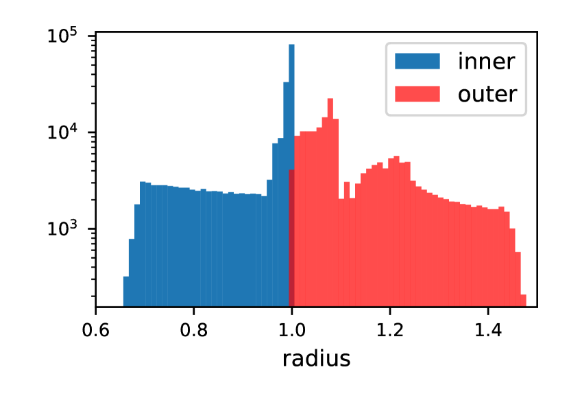
Figure 3: Histogram of the inner (in blue) and outer (in red) radii for HEALPix pixels in units corresponding to exact squares (i.e. would be one for squares). We use a logarithmic scale to emphasize the tails and determine the lower ($R_{\mathrm{in}}$) and upper ($R_{\mathrm{out}}$) values.

3.2 Homogeneous indexing

What we are interested in is indexing the sky for an efficient access of neighboring points according to some angular distance. If the shape of pixels varies too much, we are forced to use pixels that are in average too large to ensure we do not miss some neighbors on a part of the sky and the padding is unsatisfactory.

This is worsened by using hierarchical decomposition. For instance HEALPix is based on the recursive subdivision of 12 equal-area base pixels, so that the number of pixels follows $N_{\mathrm{pix}}=12\leavevmode\nobreak\ \mathtt{nside}^{2}$ where $\mathtt{nside}$ must be some integer power of 2. Then for a given angular distance cut, not only one has to use too large pixels, but their size is, furthermore, artificially increased by the fact that the resolution must be some power of 2 , which yields a rapid growth of the number of pixels. Therefore pixelizations as HEALPix, which were designed to perform power spectra estimation, are not well adapted to our indexing needs.

We then look for a more homogeneous sphere indexing with the following most constraining properties:

1. nonhierarchical decomposition,

2. small pixel inner/outer radius variations,

3. efficient “ang2pix” possibility, i.e. fast access to pixel index given a direction on the sky,

4. small (and about constant) number of pixel neighbors with efficient access to their indices.

It is worth to mention however that we do not require a strict equal-area pixelization.

As a matter of fact, nonhierarchical sphere tilings are rare nowadays. This excludes some modern pixelization schemes used in geoscience as the S2 or H3 libraries (point 1).

There exists a vast literature on the subject of locating nodes on a sphere according to some quality criteria (for a review see e.g. Hardin et al. (2016)).However pixels are most often constructed from the nodes Voronoi mesh which precludes an efficient ang2pix implementation in Spark (point 3).

A priori the most interesting pixelization would be based on hexagons, as the famous soccer ball scheme, since hexagonal pixels are very close to circles and would then show a very small radius variation. Unfortunately, it can be shown from the Euler characteristic that it is impossible to pave entirely the sphere with only hexagons; they must be complemented by exactly 12 pentagons which have unfortunately a much smaller area (0.66 of the hexagon ones). For a given angular distance cut, we would then need to adapt our tiling to the size of these pentagons losing the benefit of using hexagons (point 2).

We also exclude zonal equal array pixelizations, as the IGLOO one (Crittenden, 2000), since the poles are contained within a single pixel with a large number of neighbors (the number of meridians). They would then add artificially a large number of neighbors to the total pool which fails our 4th point.

Then we consider platonic solid projections on the sphere which turn to be well adapted to the pair counting problem. We revisit one of the simplest method based on the projection of points lying on the faces of a sphere inscribed cube, sometimes dubbed as "cubed sphere".

3.3 Cubed-Spheres

The construction of pixels on the sphere by radially projecting a grid of points from the face of a cube (see Fig.4) is a classical method for instance well described in Nair et al. (2005). The points can be positioned on a regular grid but a better strategy, still keeping simplicity, is to place them at equal angles from the origin (Rančić et al., 1996). This is our first discussed scheme. Next, a more sophisticated procedure will be revisited and evaluated.

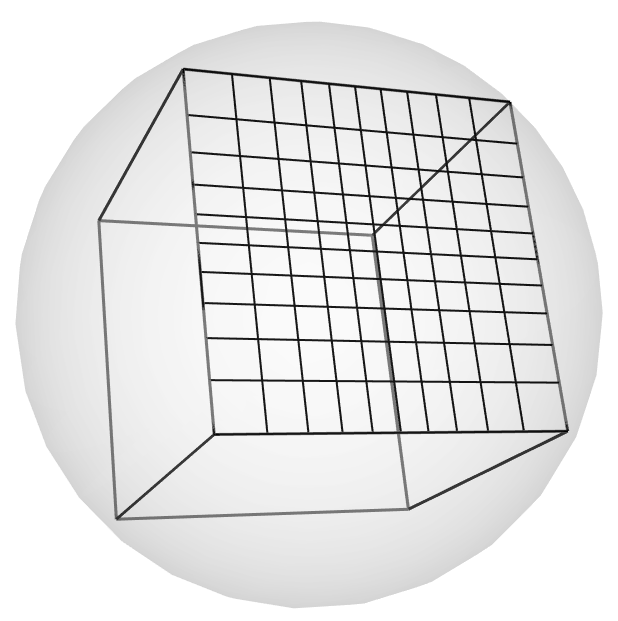
(a)

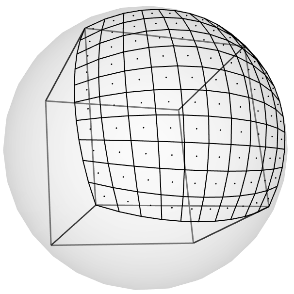
(b)

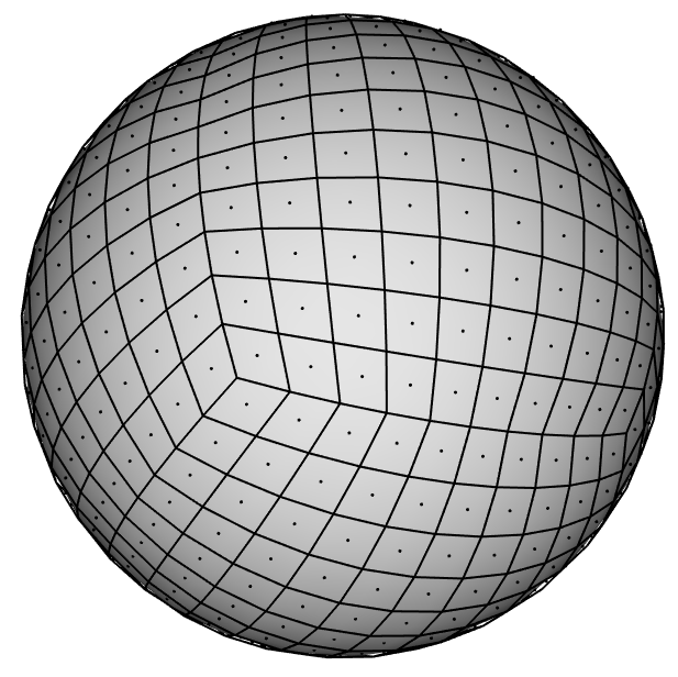
(c)

Figure 4: Steps in the construction of a cubed sphere. (a) A cube is inscribed within a unit sphere, and a grid of nodes is created on the face (here with equal angles to the center). (b) Nodes are radially projected onto the unit sphere. Four connected nodes define a pixel their barycenter defines the pixel center. (c) The process is repeated on each face using cube symmetries.

3.3.1 The equiangular case

The nodes shown on Fig.4a are located in the local plane at position

$$(x_{i},y_{j})=\tfrac{1}{\sqrt{3}}(\tan\alpha_{i},\tan\alpha_{j})$$ (10)

where the $\alpha_{i,j}$ values represent the angle from the center and are taken from a regular grid of $\mathtt{nbase}$ points over $[-\pi/4,\pi/4]$.

The number of pixels per face is thus $\mathtt{nbase}^{2}$ and their total number is

$$N_{\mathrm{pix}}=6\leavevmode\nobreak\ \mathtt{nbase}^{2}.$$ (11)

The decomposition being nonhierarchical this number can be finely tuned since $\mathtt{nbase}$ can now be any integer number.

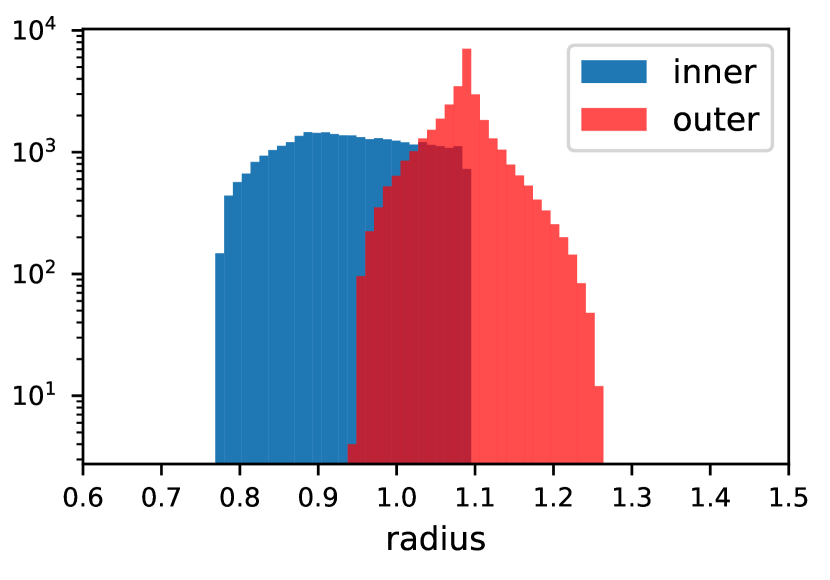
Figure 5: Histogram of the inner (in blue) and outer (in red) pixel radii for the CubedSphere pixelization normalized to values for a square.

The distributions of the inner and outer radius for this pixelization is shown on Fig.5. Compared to Fig.3, both distributions have clearly shrunk, the shape of the pixels is closer to being square. We obtain

$$\dfrac{R_{\mathrm{in}}}{R_{\mathrm{sq}}^{in}}=0.77,\quad\dfrac{R_{\mathrm{out}}}{R_{\mathrm{sq}}^{out}}=1.26$$ (12)

We have checked that this result is independent of $\mathtt{nbase}$.

3.3.2 The COBE quad-cube

The COBE cosmological microwave background pioneer mission developed an interesting sphere tiling known as the "quad cube" which is a CubedSphere projection but with a more elaborate placement of points on the face of the cube. Based on an early work by Chan & O’Neill (1975), it proceeds by mapping a regular grid of points with two invertible polynomials build to ensure almost equal-area pixels after the projection.

We have thus implemented these polynomials in our grid construction and show the effect on the pixel radii on Fig.6. We obtain

$$\dfrac{R_{\mathrm{in}}}{R_{\mathrm{sq}}^{in}}=0.78,\quad\dfrac{R_{\mathrm{out}}}{R_{\mathrm{sq}}^{out}}=1.39$$ (13)

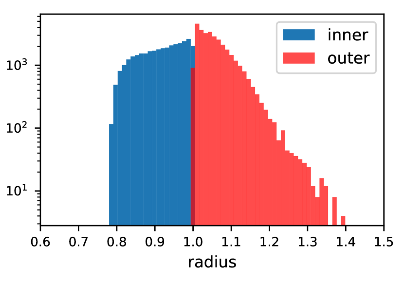
Figure 6: Histogram of the inner (in blue) and outer (in red) pixel radii for the COBE pixelization normalized to values for a square.

The outer radius distribution now shows an asymptotic tail that we traced to be related to projected pixels near the corners of the cube that have both a larger surface area and greater ellipticity (see A.2 for details). Furthermore $R_{\mathrm{out}}$ is not fully independent of the resolution (eg. one gets 1.41 for $\mathtt{nbase}$ =500). The gain on $R_{\mathrm{in}}$ with respect to the simple equiangular case is marginal.

3.4 A quasi-optimal solution: SARSPix

A smart pixelization unknown in astrophysics and cosmology was proposed by mathematicians (Lemaire & Weill, 2000) which leads both to equal-area and close-to-square pixels. Although relying on cube symmetries, it is not based on projecting a grid face, but on direct spherical computations.

However the original construction algorithm is too complex to allow a fast ang2pix implementation. In their paper, the authors exclude a simpler way to build the nodes on regular latitude bins since it does not lead to strictly equal-area pixels. Since this is not a strong constraint in our case, we have tested this simplified scheme which now allows an efficient ang2pix computation. Anticipating results, we have nicknamed it SARSPix, the Similar Radius Sphere Pixelization.

Referring for details to the original paper, we present a brief summary of the main steps in the construction process (Fig.7). One works on a quadrant of a projected cube face and define meridians that respect some regular triangular area spacing. Then one regularly splits the latitudes of each meridian up to the diagonal of the quadrant and symmetries the result with respect to it. The construction is repeated for each quadrant and face using symmetries.

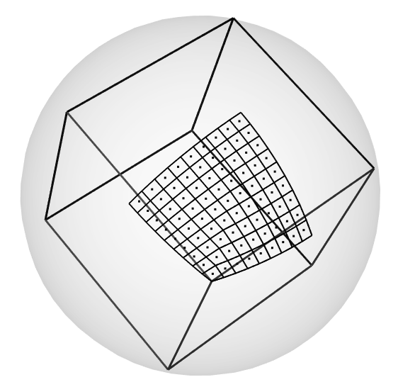
(a)

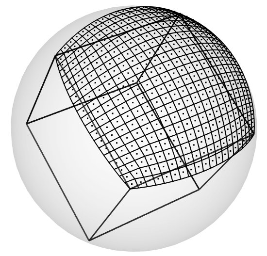
(b)

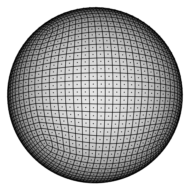
(c)

Figure 7: Construction of the SARSPix pixelization.(a) First a quadrant of a projected cube face is constructed computing the node positions directly on the sphere. (b) The other quadrants are completed using symmetries. (c) The full-sphere pixelization is completed using cube rotations.

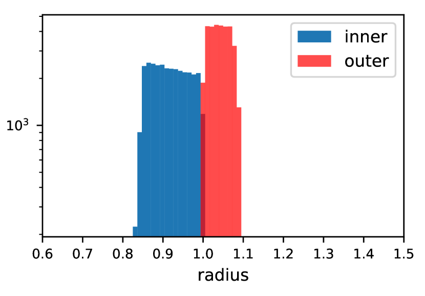
Figure 8: Histogram of the inner (in blue) and outer (in red) pixel radii for the SARSPix pixelization normalized to values for a square.

We have constructed this pixelization and show on Fig.8 the radii distribution. We obtain

$$\dfrac{R_{\mathrm{in}}}{R_{\mathrm{sq}}^{in}}=0.82,\quad\dfrac{R_{\mathrm{out}}}{R_{\mathrm{sq}}^{out}}=1.10$$ (14)

There is only a 10% departure from a square on the outer radius and about 20% on the inner one.

The total number of pixels is $N_{\mathrm{pix}}=6\leavevmode\nobreak\ \mathtt{nbase}^{2}$ where $\mathtt{nbase}$, is an even integer As for the previous cube-based pixelizations, the number of neighbors of each pixel is 8, except for the 8 cube corners where it is 7.

parameter	HEALPix	CubedSphere	SARSPix
resolution	$\mathtt{nside}=2^{N}$	$\mathtt{nbase}=N$	$\mathtt{nbase}=2N$
$N_{\mathrm{pix}}$	$12\leavevmode\nobreak\ \mathtt{nside}^{2}$	$6\leavevmode\nobreak\ \mathtt{nbase}^{2}$	$6\leavevmode\nobreak\ \mathtt{nbase}^{2}$
#neighbours	8 (7)	8 (7)	8 (7)
$R_{\mathrm{in}}$	0.65	0.77	0.82
$R_{\mathrm{out}}$	1.46	1.26	1.10

Table 2: Summary of pixelization properties studied in the text. For the resolution parameter, $N$ represents any positive integer. The number of neighbors is essentially 8 in all cases; for HEALPix there are also 24 pixels with 7 neighbors, while for cube-based constructions (CubedSphere,SARSPix) there are 8 of them (at the cube corners). $R_{\mathrm{in}}$ is the largest radius of the circles inscribed on the pixels and $R_{\mathrm{out}}$ the smallest of the circumscribed circles. They are normalized to the values for a square i.e. would be exactly 1 for square pixels.

We summarize in Table 2 the characteristics of the pixelizations that we have studied. According to our metric, which is to have the most homogeneous square-like pixels with a slowly varying resolution parameter, SARSPix is clearly superior to the others and will be our default choice both for the joining and reducing indexing.

3.5 Implementation

We have implemented the SARSPix and CubedSphere pixelizations using the Scala language and make them publicly available in the SparkCorr package The classes provide efficient access to the main functions needed by our algorithm:

1. ang2pix: $(\theta,\phi)\rightarrow\mathrm{index}$

2. pix2ang: $\mathrm{index}\rightarrow(\theta,\phi)$

3. neighbors: $\textrm{index}\rightarrow\{\textrm{indices}\}$

We evaluate the performances of the implementations by comparing them to HEALPix (java implementation) which is a very optimized code. We shoot $10^{9}$ random points over the sphere compute their index (ang2pix), then the corresponding pixel centers (pix2ang) and finally the list of all the neighbors. We have connected the Scala classes to the Spark environment and ran on 5 workers with an equivalent resolution parameter of $\mathtt{nside}$ =2048 for HEALPix and $\mathtt{nbase}$ = 2896 for CubedSphere and SARSPix. We checked that the performances are independent of the resolution. Table 3 shows the times measured for each operation. The CubedSphere and SARSPix performances are similar to the HEALPix ones but for pix2ang where the latter can determine immediately the position of the centers owing to its hierarchical decomposition but is more complicated for cube-based constructions. Storing the pixel centers in a lookup table to accelerate this function is not appropriate with Spark, since one would need to send this table to all the executors which can be long if the table is large due to the finite network bandwidth and can even saturate the heap memory. Then our pix2ang pure-function implementation relies on computing the 4 nodes and their barycenter for each point which in principle could be as long as 4 times ang2pix. The measured performances, close to the ang2pix ones, are then quite reasonable. The time increase of SARSPix over CubedSphere simply comes from the higher complexity of the former scheme. In all cases, and as will be clear in the final results, these performances are largely sufficient to not impact the full pair counting algorithm (Sect. 2.5).

operation	HEALPix	CubedSphere	SARSPix
ang2pix	26s	20s	33s
pix2ang	3s	30s	43s
neighbors	10s	15s	15s

Table 3: Time measured (in seconds) to perform the main pixelization operations on $10^{9}$ data on 5 workers (each running 32 cores).

Finally, we point out that using SARSPix we gain substantially on pair combinatorics. As an example let us consider the data reduction for a bin width of 3.2′. With HEALPix the number of pixels $N_{\mathrm{pix}}^{D}$ would be 200M ($\mathtt{nside}$ =4096) while with SARSPix we can get down to 34M ($\mathtt{nbase}$ =2386), meaning that working on a 100M dataset one cannot compress the data with the former but can obtain a factor 3 of compression with the latter. The joining pixelization is also essential for obtaining good performances. For instance, with a $\theta_{+}$ =10′upper bound, the number of pixels $N_{\mathrm{pix}}^{J}$, that decimates the pair combinatorics (Eq. (2)) is around $200.10^{3}$ with HEALPix while it is four times larger with the SARSPix indexing.

4 The DES binning scenario

4.1 Defining the setup

We use in the following the “DES binning” (Abbott et al., 2018) which consists of 20 bins uniformly spaced on a logarithmic scale from 2.5 to 250 arcmins and is detailed in Table 4. Once the binning is defined, we first work out the characteristics of the joining and reducing pixelizations for each bin.

For the joining pixelization (Sect. 2.3) we compute the smallest possible value of $\mathtt{nbase}$ which ensures that any pair of points is at an angular distance lower than $R_{\mathrm{in}}=\theta_{+}/2$ (see Fig.1). For SARSPix, using Eqs. (14),(8) and (11)

$$\mathtt{nbase}_{J}=\left\lfloor\sqrt{\dfrac{\pi}{6}}\dfrac{0.82}{R_{\mathrm{in}}}\right\rfloor$$ (15)

$\lfloor\rfloor$ indicating here the $floor$ operator, possibly adding 1 if the value is odd.

For data reduction (Sect. 2.4) the pixelization only depends on the bin width ($w$). For each bin it corresponds to the largest $\mathtt{nbase}$ value which ensures that all pixel radii are smaller than $R_{\mathrm{out}}=w/2$ (see Fig.2). For SARSPix it yields

$$\mathtt{nbase}_{D}=\left\lceil\sqrt{\dfrac{\pi}{3}}\dfrac{1.10}{R_{\mathrm{out}}}\right\rceil,$$ (16)

$\lceil\rceil$ indicating the $ceil$ operator, possibly subtracting 1 if the value is odd.

This defines the optimal pixelizations on each bin and thus the total number of pixels, assuming a full sphere coverage, $N_{\mathrm{pix}}^{D}=6\leavevmode\nobreak\ \mathtt{nbase}_{D}^{2}$ , $N_{\mathrm{pix}}^{J}=6\leavevmode\nobreak\ \mathtt{nbase}_{J}^{2}$ that are indicated in Table 4.

id	$\theta_{-}$	$\theta_{+}$	$N_{\mathrm{pix}}^{J}$ ($10^{3}$)	$w$	$N_{\mathrm{pix}}^{D}$ ($10^{6}$)
0	2.5	3.1	10,077.7	0.6	858.0
1	3.1	4.0	6,340.7	0.8	541.3
2	4.0	5.0	3,995.1	1.0	341.5
3	5.0	6.3	2,519.4	1.3	215.6
4	6.3	7.9	1,597.5	1.6	135.9
5	7.9	10.0	998.8	2.0	85.8
6	10.0	12.5	629.9	2.6	54.1
7	12.5	15.8	399.4	3.2	34.2
8	15.8	19.9	249.7	4.1	21.6
9	19.9	25.0	157.5	5.1	13.6
10	25.0	31.5	98.3	6.5	8.6
11	31.5	39.6	62.4	8.1	5.4
12	39.6	49.9	38.4	10.3	3.4
13	49.9	62.8	24.6	12.9	2.2
14	62.8	79.1	15.0	16.3	1.4
15	79.1	99.5	9.6	20.5	0.9
16	99.5	125.3	6.1	25.8	0.5
17	125.3	157.7	3.5	32.4	0.3
18	157.7	198.6	2.4	40.8	0.2
19	198.6	250.0	1.5	51.4	0.1

Table 4: Setup used with the DES binning. The first column is an identifier used to define bin ranges. Then comes the bin $[\theta_{-},\theta_{+}]$ boundaries (in arcmins) and $N_{\mathrm{pix}}^{J}$ the associated number of pixels (in thousands) of the joining pixelization that depends only on $\theta_{+}$. Then comes $w$ the bin width (arcmins) and its associated number of pixels for the data reduction $N_{\mathrm{pix}}^{D}$ (in millions).

Note that pixel reduction is not always efficient on the first bins. For instance, for 100M input data, there are actually more pixels in the first 5 bins so it makes no sense using it. One could then trigger it only when $N_{\mathrm{pix}}^{D}<\textrm{N}_{\mathrm{data}}$.

However Spark allows much more data to be processed at once. We work in the following on bin ranges defined by a pair of identifiers from Table 4 as $[i_{min},i_{max}]$. We can then use the joining pixelization corresponding to $\theta_{+}(i_{max})$ for all the range since by construction all lower index values have a lower angular separation. Conversely, for data reduction (if any) we can use the pixelization corresponding to $w(i_{min})$ since the width increases with the bin number. Then we use some fixed-size pixelizations with $N_{\mathrm{pix}}^{J}(_{max})$ and $N_{\mathrm{pix}}^{D}(i_{min})$ pixels, the latter being optional. It is important to notice that the fact that $\theta_{+}$ and $w$ evolve one against the other, allows treating the full histogram with very little ranges since when $N_{\mathrm{pix}}^{J}$ increases $N_{\mathrm{pix}}^{D}$ decreases and the number of pairs becomes easily tractable (Eq. (7)). In practice it means we need to run very little jobs on a cluster. The optimal slicing depends on the binning, the data size and cluster performances, but we will see that to complete the full DES histogram on $10^{8}$ to $10^{9}$ data points we only need 2 to 4 bin ranges (i.e. jobs).

4.2 Data and infrastructure

To study performances on a large and realistic dataset we used the CoLoRe software that is a fast simulation populating point-like galaxies according to a log-normal over-density distribution. We built a catalog of around 6 billions of galaxies corresponding to 10 years of LSST observations and extract three datasets by filtering galaxies with a redshift between 1 and an upper cut chosen to create different size catalogs, the “100M”, “500M” and “1G” ones containing respectively $10^{8},5.10^{8}$ and $10^{9}$ point-like galaxies distributed over the full sky.

The tests were run at the NERSC computing center on the Spark 2.4.4 version. Each job provides to Spark a number of sandboxed workers corresponding to the number of nodes specified by the user . Each node has two sockets, each socket being populated with a 2.3 GHz 16-core Haswell processor (Intel Xeon Processor E5-2698 v3). Each node has 100 GB memory, about 60% being used for the cache. Even if NERSC proposes high-quality supercomputer services, we emphasize that this is not essential here since Spark is by design a framework to be run on any data center. Some results on Spark performances at NERSC are reported in Peloton et al. (2018).

4.3 Performances

4.3.1 The exact method

The most demanding part of the algorithm is when the data reduction cannot be applied which occurs for the first angular distance bins, i.e. when $N_{\mathrm{pix}}^{D}$ exceeds the input data size. The first bin range $[0,i_{max}]$ could then go up to where the compression starts becoming effective ($N_{\mathrm{pix}}^{D}<\textrm{N}_{\mathrm{data}}$). It would lead for example to $i_{max}=4$ on the 100M sample (Table 4). As discussed in the previous part, we can be more ambitious with Spark and push $i_{max}$ higher. To estimate up to where we can go, we consider the theoretical number of pairs Eq. (2). Using $N_{\mathrm{pix}}^{J}$ from Table 4 we represent $N_{\textrm{pairs}}^{X}$according to $i_{max}$ on Fig.9 for the three datasets.

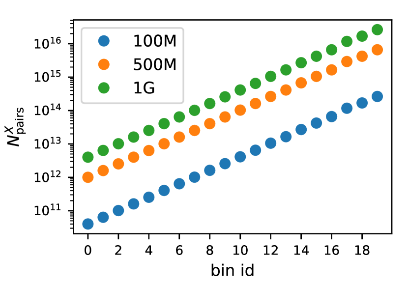
Figure 9: Theoretical number of pairs with the exact method from bin 0 to the shown identifier (from Table 4) on our three datasets.

In order to obtain results within minutes, we found that Spark at NERSC can handle up to about $10^{13}$ pairs. By consequences, we have chosen $i_{max}=10,5$ and $1$ for the "100M", "500M" and "1G" datasets, respectively. Note that from this figure one can adjust the bin range to other cluster performances.

$\textrm{N}_{\mathrm{data}}$	bin range	nodes	$N_{\textrm{pairs}}^{X}$	wall time (mins)
$10^{8}$	[0,10]	16	$4.10^{12}$	$1.7\pm 0.1$
$5.10^{8}$	[0,5]	32	$10^{13}$	$2.4\pm 0.1$
$10^{9}$	[0,1]	64	$6.10^{12}$	$1.7\pm 0.1$

Table 5: Timing results on the first bin range (Table 4) for the three datasets ("100M", "500M" and "1G") with the exact method. We also give the number of nodes used and the theoretical number of pairs computed from Eq. (2).

Table 5 shows the timing results obtained running five jobs each time to measure the average and standard deviation. Starting with 16 nodes, we doubled each time their number in particular to hold the increasing data in the cache, which will be discussed in more details later. In each case a wall time of about 2 minutes is achieved.

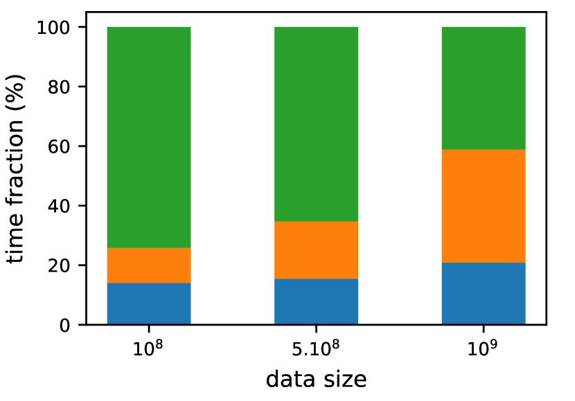
Figure 10: Relative time spent in the main steps described in the text of the exact algorithm for Table 5 setup. Following Sect. 2.5 terminology, in blue the source part, in orange the duplicates one and in green the join one.

Let us investigate where time is spent. Using Sect. 2.5 terminology, we show on Fig.10 the relative time spend in the main parts of the algorithm. For the "100M" and "500M" datasets most of the time is spent in performing the combinatorics (the join part, point 3 in Sect. 2.5)). For the "1G" dataset, the duplicates part (point 2 in Sect. 2.5) is increasing since one has to repartition and put in cache about 500 GB of data and is therefore limited by the network bandwidth.

Putting data in cache boosts the join part of the algorithm but one does not always have access to a cluster with such a high level of in-cache memory. So we removed the cache usage in both the source and duplicates steps and measure $2.6$ mins on the "1G" dataset. This is a minor increase with respect to $1.7$ mins obtained using the cache, showing that its usage is not mandatory.

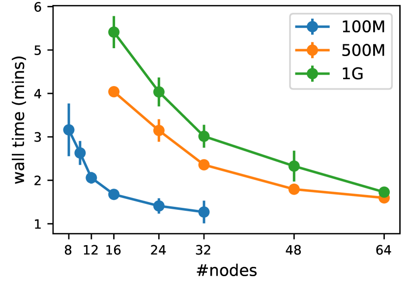
Figure 11: Time measured on our datasets with the exact method varying the number of nodes. Results are averaged over 5 runs for each point.

We then study how performances vary with the number of workers (nodes). Results are presented on Fig.11. The code scales nicely up to about 12 nodes on the "100M" sample and 32 for the "500M" and "1G" ones. The time is already at the 1-2 minutes level that adding more nodes reveal some Spark overheads (as putting data in the cache) although one still gets a small improvement.

4.3.2 The reduced method

When the bin number increases, $N_{\mathrm{pix}}^{J}$ decreases (see Table 4) and combinatorics increases too, but at the same time one can apply the data reduction method (step 0 in sectsec:overview) and replace the dataset by $N_{\mathrm{pix}}^{D}$ cells keeping the number counts (Sect. 2.4).

Then, as in the previous section, one needs to decide the size of the bin range that will be processed. Let us illustrate it on the "1G" dataset. Bins 0 to 1 were already treated by the exact method, so we start at $i_{\mathrm{min}}$=2. This fixes the maximal bin width and therefore the size of the reducing pixelization. From Table 4 one reads $N_{\mathrm{pix}}^{D}$, which is here about 340 million. We then look for the lowest possible bin for which $N_{\mathrm{pix}}^{J}$ gives a number of combinations Eq. (7) that stays "small" (below $10^{13}$), which lead us to choose $i_{\mathrm{max}}$=5. We then proceed in the same way for next bins.

In this way, we obtain 3 bin ranges (jobs) for the "1G" dataset ([2,4], [5,10] and [11,19]) , 2 for the "500M" one ([6,10] and [11,19]) and a single range ([11-19]) for the "100M" case. In most cases the combinatorics is actually small $(N_{\mathrm{pix}}^{D})^{2}/N_{\mathrm{pix}}^{J}\ll 10^{11}$ so we use 16 nodes everywhere but for the "1G" case for which the [2,4] index range is slightly heavier and requires 32 nodes.

Timing results are shown in Table 6. With 1 to 2 minutes, they are even better than those obtained with the exact method

After optimization, the time spend in the Reduction stage (step 0 in Sect. 2.5) becomes negligible so that the total time on a given bin range becomes independent of the initial data size. This can be seen in Table 6 on the [11,19] bin range case for which the processing time is the same whatever the dataset size is.

$\textrm{N}_{\mathrm{data}}$	bin range	$N_{\textrm{pairs}}^{R}$	time (mins)
$10^{8}$	[11,19]	$8.10^{11}$	$0.9\pm 0.1$
$5.10^{8}$	[6,10]	$10^{12}$	$1.1\pm 0.2$
	[11,19]	$8.10^{11}$	$0.9\pm 0.2$
$10^{9}$	[2,4]	$3.10^{12}$	$2.1\pm 0.3$
	[5,10]	$3.10^{12}$	$2.3\pm 0.4$
	[11,19]	$8.10^{11}$	$0.9\pm 0.1$

Table 6: Timing results obtained on the three datasets with the reduced method. Independent jobs are run over different bin ranges to finalize results obtained with the exact algorithm (Table 5). We give the estimated number of pairs from Eq. (7) computed from Table 4 taking for $N_{\mathrm{pix}}^{D}$ the low bin value and for $N_{\mathrm{pix}}^{J}$ the high one. Sixteen nodes were used everywhere but for the $10^{9}$ [2,4] case where it is 32.

4.3.3 Combination and cross-checks

Using both the exact and reduced independent methods (Secs. 4.3.1, 4.3.2) , one can then reconstruct the full histogram in about 2 minutes by launching 2, 3, 4 jobs on the "100M", "500M" and the "1G" datasets, respectively.

We undertake some tests to check the coherence of the results in particular on the pixelization resolution side to verify that we collected all the pairs. To do so, we use the "100M" sample and first perform a reference run with the exact method on a very large [0,15] bin range. The $i_{\mathrm{max}}=15$ bound being very high, the pixel size over which the join is performed is very large ($\mathtt{nbase}_{J}$ = 40). This run took about 8 minutes on 64 nodes. Then, we compare the number of pairs reconstructed up to bin 10 against our default implementation that fixes the pixelization according to Eq. (15) which had a much smaller resolution ($\mathtt{nbase}_{J}$ =128) Results are shown in Table 7 and indicate a very good agreement between the two methods: they are exactly the same up to bin 8 and differ by $10^{-6}$ for bin 10, showing that our joining pixel size (Eq. (15)) is well adapted to the problem.

id	$N_{ref}$	$N_{def}^{\tt exact}$
0	506727642	506727642
1	800041282	800041282
2	1260509592	1260509592
3	1979959475	1979959475
4	3096818992	3096818992
5	4815924052	4815924052
6	7438665544	7438665544
7	11411877241	11411877241
8	17425875136	17425875136
9	26591445306	26591444936
10	40723594728	40723260295

Table 7: Number of pairs measured on the $10^{8}$ sample with the exact method with the reference and default setup

We know that the compression applied in the reduced method is not absolutely lossless (Eq. (5)). There is a slight smearing around the binning boundaries which is difficult to predict. In order to study this effect, two jobs have been launched with the reduced method on the [5,10] and [10,15] bin ranges. We then compare the values obtained with those of our reference run that is exact. The results shown in Table 8 shows that the precision of the reduced method is at the $10^{-3}$ level

id	$N_{ref}$	$N_{def}^{\tt reduced}$	rel. error
5	4815924052	4820614147	-0.00097
6	7438665544	7436640102	0.00027
7	11411877241	11353806206	0.00509
8	17425875136	17448008463	-0.00127
9	26591445306	26579894562	0.00043
10	40723594728	40730263699	-0.00016
10	40723594728	40767727583	-0.00108
11	62746460926	62752402410	-0.00009
12	97293945900	96819343446	0.00488
13	151684971831	151890299528	-0.00135
14	237573071187	237474741141	0.00041
15	373467108791	373494164330	-0.00007

Table 8: Number of pairs measured with the reference setup and two reduced runs ([5,10] and [10,15] bin ranges in Table 4) and relative fraction between them.

5 Conclusion

We have shown how to perform pair-counting on a standard logarithmically binned histogram, up to one billion input data in about two minutes using the Spark big data technology. The algorithm we developed uses standard functions on dataframes and was shown to scale with the number of nodes. This demonstrate that Spark, although not very used in the astrophysics community, is a valuable tool to handle very large combinatorics.

To achieve this level of performance we have revisited the non-hierarchical sphere pixelization and propose a new one, SARSPix (Sect. 3.4) that indexes the sky with regular shape quadrangles. While HEALPix is widely used in astrophysics, SARSPix is much more adapted to all operations involving some local search over the sphere.

Although some sate-of-the-art HPC implementation of pair counting algorithm (as is done in treecorr) can achieve similar performances, they do it thanks to an evolved algorithm (and approximations) not data structure. There are two advantages in exploring a Spark implementation. First, the big data approach allows an optimized “ brute-force” computation up to quite large separation angles, meaning the results are exact. Once the full set of pairs is reconstructed the binning process itself is light, meaning that any binning (as a linear one) gives similar performances Second, the main difference with a state-of-the-art implementation written by expert(s) is that the data structure (a dataframe) and algorithm (indexing on the sphere and join) is much simpler. With little effort and no knowledge about parallel computing, any user can obtain performances similar to the most specialized software on this high combinatorics problem. With little adaptation one can also address other problems related to local distance computations as:

• k-NN nearest neighbor search,

• cross-match between two catalogs,

• cluster building with some linking length (as the “ friend of friends” method used for instance in N-body simulations to reconstruct halos).

And of course the method can be adapted straightforwardly to the Euclidian case where indexing is provided simply by binning each dimension. Although we presented timing results on a super-computer we remind that it is not a necessary requirement since Spark is in essence designed to be run on any set of connected computers.

Data availability

The data used to produce the results as described in Sect.4.2 are publically available at https://me.lsst.eu/plaszczy/scalingpaircount. They consist in 4 tar-compressed parquet files:

tomo1M.parquet.tar, tomo100M.parquet.tar,
tomo500M.parquet.tar, tomo1GB.parquet.tar

corresponding respectively to the $10^{6},10^{8}$, $5.10^{8}$ and $10^{9}$ sample datasets. The complete size is of 12 GB. For an initiation on a personal laptop, you can just grab and untar the tomo1M.parquet file and follow for instance the example of Sect. 2.1. You need a working pyspark implementation which can be downloaded from https://spark.apache.org/downloads.html.

Appendix A Pixelization properties

We give in this appendix more details about the cube-based pixelizations discussed in the text. In each case we have built the nodes of the pixelization for one face (the other being equivalent by symmetry) and study some properties of the pixels determined from the four delimiting nodes :

• Area,

• ellipticity $\left|\tfrac{p-q}{p+q}\right|$ , $p,q$ being the diagonal lengths,

• outer radius (of the circumscribed circle) ,

• inner radius (of the inscribed circle).

In all cases we used exact formulas for quadrilaterals. The area and ellipticity are deeply related to the radii since having a large area together with a large ellipticity directly impacts the distance of the center to its corners, thus the outer radius.

A.1 CubedSphere

Fig.12 shows the results of the CubedSphere pixelization for $\mathtt{nbase}$ =180. We normalize all our values to those of squares (Eq. (8)) so that $R_{\mathrm{in}}$, $R_{\mathrm{out}}$ and the area would be exactly 1 for square pixels and of ellipticity 0.

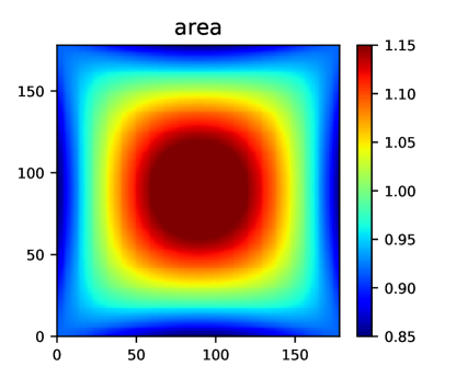
(a)

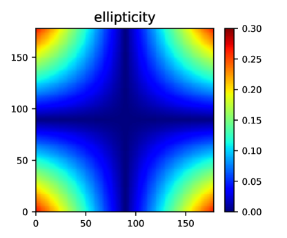
(b)

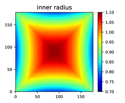
(c)

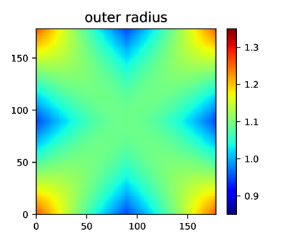
(d)

Figure 12: Properties of the CubedSphere pixels. Indices run over one face of the projected cube ($\mathtt{nbase}$ =180) and values are normalized to those of a square i.e. would be exactly 1 for the area, inner and outer radii, 0 for ellipticity.

The pixel area varies by 10% and decreases near the corners. The ellipticity increases near the corners corner.

A.2 COBE

The same properties are studied on Fig.13 using the COBE mapping of the points on the face which was designed to obtain almost equal areas.

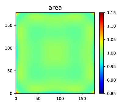
(a)

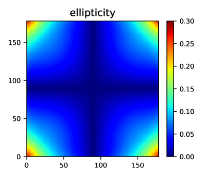
(b)

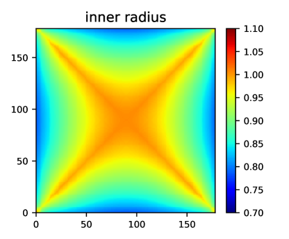
(c)

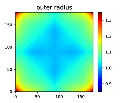
(d)

Figure 13: Properties of the COBE pixels. Indices run over one face of the projected cube ($\mathtt{nbase}$ =180) and values are normalized to those of a square i.e. would be exactly 1 for the area, inner and outer radii, 0 for ellipticity.

Indeed the pixel area becomes very uniform (below 1% as was claimed) but near the corners where a $\simeq 7$% excess is observed. The ellipticity is also globally closer to 0 but also increases near the corners. The product of both effects lead to a dramatic increase in the outer radius near the cube corners that was observed on Fig.6. The inner radius is globally better than on Fig.12 but its lowest value ($R_{\mathrm{in}}$) is about the same than for CubedSphere.

A.3 SARSPix

SARSPix is a very different pixelization that does not project points of the cube to the sphere but performs directly spherical computations. However since it relies on cube symmetries, one can still index pixels in the same way as previously. We show the results on Fig.14.

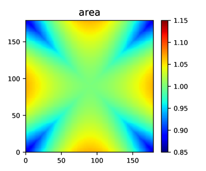
(a)

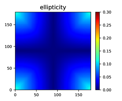
(b)

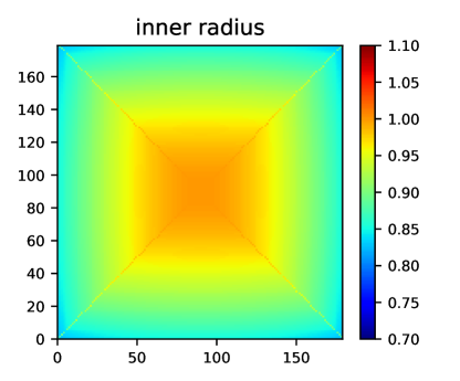
(c)

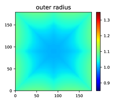
(d)

Figure 14: SARSPix properties. Indices run over the face of a ($\mathtt{nbase}$ =180) and values are normalized to those of a square i.e. would be exactly 1 for the area, inner and outer radii, 0 for ellipticity

The pixel area is less uniform than in the COBE case but decreases near the corner. The ellipticity is excellent and interestingly slightly increases near the corner: the product of both effects leads to an excellent outer radius that does not increase on the corners. The inner radius is also very good, the cross appearing here being due to the symmetrization along the diagonals which can be spotted on Fig.7a.

References

- Abbott et al. (2018) Abbott, T. M. C., Abdalla, F. B., Alarcon, A., et al. 2018, Phys. Rev. D, 98, 043526, doi: 10.1103/PhysRevD.98.043526
- Alonso (2013) Alonso, D. 2013, CUTE solutions for two-point correlation functions from large cosmological datasets. https://arxiv.org/abs/1210.1833
- Armbrust et al. (2015) Armbrust, M., Xin, R. S., Lian, C., et al. 2015, in Proceedings of the 2015 ACM SIGMOD International Conference on Management of Data, SIGMOD ’15 (New York, NY, USA: ACM), 1383–1394, doi: 10.1145/2723372.2742797
- Asgari et al. (2020) Asgari, M., Lin, C.-A., Joachimi, B., et al. 2020, arXiv e-prints, arXiv:2007.15633. https://arxiv.org/abs/2007.15633
- Brahem et al. (2018a) Brahem, M., Yeh, L., & Zeitouni, K. 2018a, in Proceedings of the 26th ACM SIGSPATIAL International Conference on Advances in Geographic Information Systems, SIGSPATIAL 2018, Seattle, WA, USA, November 06-09, 2018, 229–238, doi: 10.1145/3274895.3274942
- Brahem et al. (2018b) Brahem, M., Zeitouni, K., & Yeh, L. 2018b, IEEE Transactions on Big Data, 1, doi: 10.1109/TBDATA.2018.2873749
- Chan & O’Neill (1975) Chan, F., & O’Neill. 1975, Computer Sciences Corp., EPRF Tech. Report, 2-75
- Crittenden (2000) Crittenden, R. G. 2000, Astrophysical Letters and Communications, 37, 377. https://arxiv.org/abs/astro-ph/9811273
- Dean & Ghemawat (2008) Dean, J., & Ghemawat, S. 2008, Communications of the ACM, 51, 107
- Górski et al. (2005) Górski, K. M., Hivon, E., Banday, A. J., et al. 2005, ApJ, 622, 759, doi: 10.1086/427976
- Hardin et al. (2016) Hardin, D. P., Michaels, T. J., & Saff, E. B. 2016, A Comparison of Popular Point Configurations on . https://arxiv.org/abs/1607.04590
- Hikage et al. (2019) Hikage, C., Oguri, M., Hamana, T., et al. 2019, PASJ, 71, 43, doi: 10.1093/pasj/psz010
- Hong et al. (2020) Hong, S., Jeong, D., Hwang, H. S., et al. 2020, MNRAS, 493, 5972, doi: 10.1093/mnras/staa566
- Jarvis et al. (2004) Jarvis, M., Bernstein, G., & Jain, B. 2004, MNRAS, 352, 338–352, doi: 10.1111/j.1365-2966.2004.07926.x
- Kilbinger (2015) Kilbinger, M. 2015, Reports on Progress in Physics, 78, 086901, doi: 10.1088/0034-4885/78/8/086901
- Laureijs et al. (2011) Laureijs, R., Amiaux, J., Arduini, S., et al. 2011, arXiv e-prints, arXiv:1110.3193. https://arxiv.org/abs/1110.3193
- Lemaire & Weill (2000) Lemaire, C., & Weill, J. 2000, in Proceedings of the 12th Canadian Conference on Computational Geometry, Fredericton, New Brunswick, Canada, August 16-19, 2000, 227–232
- LSST Science Collaboration et al. (2009) LSST Science Collaboration, Abell, P. A., Allison, J., et al. 2009, arXiv e-prints, arXiv:0912.0201. https://arxiv.org/abs/0912.0201
- Mandelbaum (2018) Mandelbaum, R. 2018, ARA&A, 56, 393, doi: 10.1146/annurev-astro-081817-051928
- Meng et al. (2015) Meng, X., Bradley, J., Yavuz, B., et al. 2015, arXiv e-prints, arXiv:1505.06807. https://arxiv.org/abs/1505.06807
- Möller et al. (2020) Möller, A., Peloton, J., Ishida, E. E. O., et al. 2020, MNRAS, 501, 3272, doi: 10.1093/mnras/staa3602
- Nair et al. (2005) Nair, R. D., Thomas, S. J., & Loft, R. D. 2005, Monthly Weather Review, 133, 814, doi: 10.1175/MWR2890.1
- Peebles (1980) Peebles, P. J. E. 1980, The large-scale structure of the universe (Princeton University Press)
- Peloton et al. (2018) Peloton, J., Arnault, C., & Plaszczynski, S. 2018, Computing and Software for Big Science, 2, 7, doi: 10.1007/s41781-018-0014-z
- Plaszczynski et al. (2019) Plaszczynski, S., Peloton, J., Arnault, C., & Campagne, J. 2019, Astronomy and Computing, 28, 100305, doi: https://doi.org/10.1016/j.ascom.2019.100305
- Rančić et al. (1996) Rančić, M., Purser, R. J., & Mesinger, F. 1996, Quarterly Journal of the Royal Meteorological Society, 122, 959, doi: 10.1002/qj.49712253209
- Zaharia et al. (2010) Zaharia, M., Chowdhury, M., Franklin, M. J., Shenker, S., & Stoica, I. 2010, in Proceedings of the 2Nd USENIX Conference on Hot Topics in Cloud Computing, HotCloud’10 (Berkeley, CA, USA: USENIX Association), 10–10. http://dl.acm.org/citation.cfm?id=1863103.1863113
- Zaharia et al. (2012) Zaharia, M., Chowdhury, M., Das, T., et al. 2012, in Presented as part of the 9th USENIX Symposium on Networked Systems Design and Implementation (NSDI 12) (San Jose, CA: USENIX), 15–28. https://www.usenix.org/conference/nsdi12/technical-sessions/presentation/zaharia
- Zečević et al. (2018) Zečević, P., Slater, T. C., Lončarić, S., & Jurić, M. 2018, in BigSkyEarth conference: AstroGeoInformatics, Tenerife, Spain, December 17-19, 2018 (Zenodo), doi: 10.5281/zenodo.1453862