Paths to caustic formation in turbulent aerosols

Abstract

The dynamics of small, yet heavy, identical particles in turbulence exhibits singularities, called caustics, that lead to large fluctuations in the spatial particle-number density, and in collision velocities. For large particle, inertia the fluid velocity at the particle position is essentially a white-noise signal and caustic formation is analogous to Kramers escape. Here we show that caustic formation at small particle inertia is different. Caustics tend to form in the vicinity of particle trajectories that experience a specific history of fluid-velocity gradients, characterised by low vorticity and a violent strain exceeding a large threshold. We develop a theory that explains our findings in terms of an optimal path to caustic formation that is approached in the small inertia limit.

Ensembles of heavy particles in turbulence, such as water droplets in turbulent clouds [1] or dust grains in the turbulent gas of protoplanetary disks [2, 3], may exhibit large fluctuations of the particle-number density and of their relative velocities [4, 5, 6, 7]. These fluctuations are enhanced by the formation of caustics [8, 9, 10], i.e., folds of the particle distribution over configuration space. Caustic formation is an effect of particle inertia, driven by the fluid-velocity gradients, that gives rise to a multivalued particle-velocity field. Due to this multivaluedness, often called the ‘sling effect’ [11, 12], particles may approach each other, and possibly collide, at large relative velocities. Accordingly, caustics have an important impact on the distribution of relative velocities [13, 14, 15, 16], and are a crucial ingredient to theories for collision rates and collision outcomes [17, 18, 19]. In effect, caustic formation may increase the variance of the particle size distribution in turbulent aerosols because, on the one hand, caustics facilitate particle growth by enhancing collision rates [14, 16]. Increased collision velocities may, on the other hand, lead to fragmentation, and thus to reduced particle sizes [3].

Caustics have been extensively studied in direct numerical simulations (DNSs) of particles in turbulence [12] and model flows [20, 21, 22, 9, 23, 24, 25]. Recent numerical studies [26, 27] found that high-velocity collisions tend to occur where the turbulent strain is large, but this cannot be explained in terms of the white-noise models usually used to study caustic formation [8, 9, 10]. A precise understanding of how caustics form at small particle inertia, including the local flow conditions that lead to their formation, is crucial for the identification of caustics in experiments [28] and for sampling them efficiently in DNS [12].

In this Letter, we describe a significant step towards a detailed understanding of how caustics form in turbulence. Using a DNS of two-dimensional turbulence, we show that whether a caustic forms or not depends on the history of the fluid-velocity gradients experienced by closeby particles, not just upon instantaneous correlations between particle positions and flow gradients (preferential concentration [29, 30, 7]). When particle inertia is small, we find a most likely history, i.e., an “optimal path” to caustic formation. To determine this path is an optimal-fluctuation problem, similar in nature to localisation due to optimal potential fluctuations in disordered conductors [31], population extinction due to environmental and population-size fluctuations [32, 33], and shock formation in Burgers turbulence [34, 35].

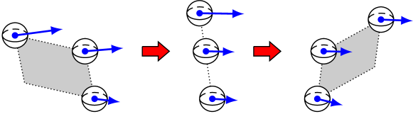
Figure 1: Illustration of caustic formation in two spatial dimensions. Shown are three nearby particles. A caustic is formed when faster particles overtake slower ones. At a caustic, the area $\mathscr{\hat{V}}$ of the parallelepiped spanned by separation vectors between the three particles, shown in grey, vanishes.

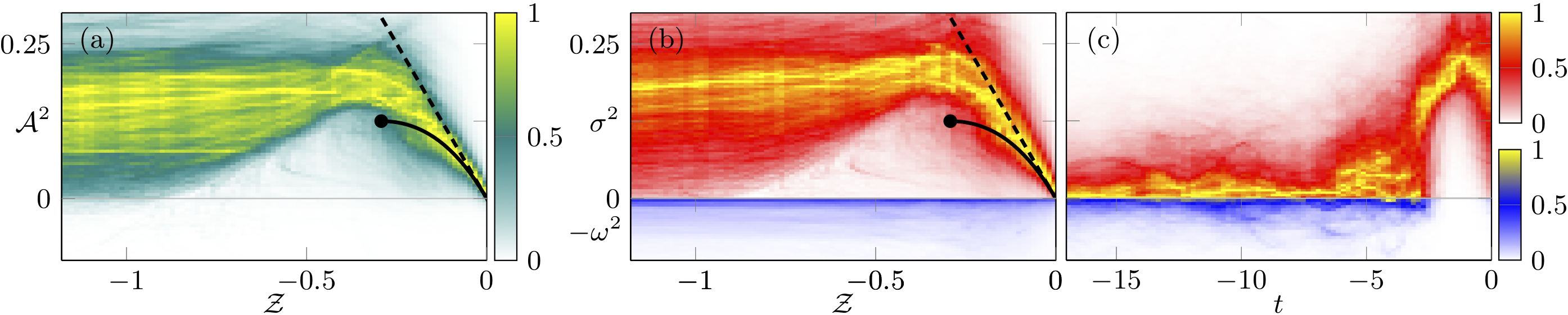
Figure 2: Path to caustic formation for $\mbox{St}=0.31$. Numerical results using a DNS of two-dimensional turbulence. The path density is colour coded, normalised to unity along each slice of constant $\mathcal{Z}$ to improve visibility. (a) Path density in the $\mathcal{Z}$-$\mathcal{A}^{2}$ plane. The dashed line shows the approximation, $\mathcal{Z}\sim\mathcal{A}^{2}$. The solid line shows the evolution of the stable fixed point according to Eq. (6). The dot marks the bifurcation to instability (see main text). (b) Individual contributions from strain ($\mathcal{Z}$ vs $\sigma^{2}$, positive axis) and vorticity ($\mathcal{Z}$ vs $-\omega^{2}$, negative axis). (c) Path densities for $\sigma^{2}$ (positive axis) and $-\omega^{2}$ (negative axis) as a function of time before caustic formation at $t=0$.

Based on this observation, we develop a theory that explains how the strain and vorticity change along the optimal path to caustic formation: The fluid strain performs a time-localised, violent fluctuation that exceeds a large threshold, while vorticity remains small. Our results explain qualitatively why DNSs of particles in turbulence show increased collision rates in straining regions [26, 27]. Even at finite inertia, the optimal path leaves a clear mark in the data, providing criteria for the identification and the efficient sampling of caustics in experiments and in DNSs.

In a dilute suspension of small, heavy, spherical particles, the dynamics of a single particle is approximately given by Stokes’ law [7],

$$\tfrac{\text{d}}{\text{d}t}\mbox{\boldmath$x$}(t)=\mbox{\boldmath$v$}(t)\,,\quad\tfrac{\text{d}}{\text{d}t}\mbox{\boldmath$v$}(t)=\tau_{\text{p}}^{-1}\{\mbox{\boldmath$u$}[\mbox{\boldmath$x$}(t),t]-\mbox{\boldmath$v$}(t)\}\,.$$ (1)

Here, $x$ and $v$ denote particle position and velocity; $\tau_{\text{p}}=2a^{2}\rho_{\text{p}}/(9\rho_{\text{f}}\nu)$ is the particle-relaxation time which depends on the particle size $a$, the kinematic viscosity $\nu$ of the fluid, and the particle and fluid densities, $\rho_{\text{p}}$ and $\rho_{\text{f}}$, respectively. The turbulent fluid-velocity field, evaluated at the particle position, is denoted by $\mbox{\boldmath$u$}[\mbox{\boldmath$x$}(t),t]$.

To describe caustic formation, we consider the parallellepiped spanned by $d+1$ nearby particles in $d$ spatial dimensions. How the spatial volume $\mathscr{\hat{V}}(t)$ of this object contracts or expands under the nonlinear dynamics (1) is determined by the spatial Jacobian $J_{ij}[\mbox{\boldmath$x$}(t_{0}),t]=\partial x_{i}(t)/\partial x_{j}(t_{0})$, namely, $\mathscr{\hat{V}}(t)=|\det\mathbb{J}(t)|$. Since the dynamics (1) takes place in $2d$-dimensional phase space, spatial subvolumes $\mathscr{\hat{V}}$ may collapse in finite time, $\mathscr{\hat{V}}\to 0$, when a caustic forms [7]. Figure 1 shows a typical particle configuration that leads to a caustic in two spatial dimensions. As is well known, caustic formation is closely related to the dynamics of the particle-velocity gradients, which reads, in dimensionless form [11, 7],

$$\mbox{St}\tfrac{\text{d}}{\text{d}t}{\mathbb{Z}}(t)=-\mathbb{Z}(t)-\mathbb{Z}(t)^{2}+\mathbb{A}(t)\,,$$ (2)

with initial condition $\mathbb{Z}(t_{0})=\mathbb{A}(t_{0})$. Here, the Stokes number $\mbox{St}=\tau_{\text{p}}/\tau_{\text{K}}$ is a dimensionless measure of particle inertia; $Z_{ij}=\tau_{\text{p}}\partial v_{i}(t)/\partial x_{j}(t)$ and $A_{ij}=\tau_{\text{p}}\partial u_{i}(t)/\partial x_{j}(t)$ are the dimensionless matrices of particle-velocity gradients and fluid-velocity gradients, respectively. In Eq. (2), time is dedimensionalised by the Kolmogorov time, $\tau_{\text{K}}^{2}=\langle\sum_{i,j=1}^{2}(\partial u_{i}/\partial x_{j})^{2}\rangle_{s}=\tau_{\text{p}}^{2}\langle\mbox{Tr}(\mathbb{AA}^{\sf T})\rangle_{s}$, where $\langle\cdot\rangle_{s}$ denotes a steady-state ensemble average. Here and in the following, we use the abbreviations $\mathbb{Z}(t)=\mathbb{Z}[\mbox{\boldmath$x$}(t),t]$ and $\mathbb{A}(t)=\mathbb{A}[\mbox{\boldmath$x$}(t),t]$. Using (2), one finds [7]

$$\mathscr{\hat{V}}(t)=\mathscr{\hat{V}}(t_{0})\exp\int^{t}_{t_{0}}\!\!{\rm d}s\,\mathcal{Z}(s)\,,$$ (3)

where $\mathcal{Z}=\mbox{Tr}\mathbb{Z}$ is the divergence of the field of particle-velocity gradients. Hence, a necessary condition for caustic formation is that $\mathcal{Z}$ escapes to negative infinity.

Apart from the Reynolds number Re that specifies the turbulence intensity, the particle dynamics is determined by the Stokes number St. For small St, particle detachment is characterised by $\mathbb{A}-\mathbb{Z}$, which is typically of the order of St, and thus small. Caustic formation requires the activation of the nonlinear term in Eq. (2) that drives the particle-velocity gradients into a caustic. This, in turn, requires rare and violent fluctuations of the fluid-velocity gradients $\mathbb{A}$ of the order of unity.

We determine the dominant events that drive caustic formation by measuring the statistics of paths in the joint space of $\mathcal{Z}$ and the fluid velocity gradients $\mathbb{A}$. In isotropic turbulence, the properties of any statistical quantity must be invariant under rotations. In addition to $\mathcal{Z}$, we therefore map out the paths of the invariants obtained from the symmetric ($\mathbb{S}$) and antisymmetric ($\mathbb{O}$) parts of the fluid-velocity gradient matrix $\mathbb{A}$: $\omega^{2}=\mbox{Tr}\mathbb{OO}^{\sf T}$ and $\sigma^{2}=\mbox{Tr}\mathbb{SS}^{\sf T}$. Figure 2 shows the paths to caustic formation obtained by numerical simulation, using a DNS of two-dimensional incompressible turbulence. Our simulations are performed in a periodic box forced at the large scales, in the regime of direct cascade of enstrophy. A drag-friction term ensures steady-state turbulence; see the Supplemental Material (SM) for more details. The path density in Fig. 2 is colour coded, with the highest densities shown in yellow.

Figure 2(a) shows paths to caustic formation in the $\mathcal{Z}-\mathcal{A}^{2}$ plane, where $\mathcal{A}^{2}=\sigma^{2}-\omega^{2}=\mbox{Tr}(\mathbb{A}^{2})$ is the Okubo-Weiss parameter [37, 38] that discerns hyperbolic from elliptic regions in the flow. We see that most paths (yellow regions) that reach a caustic at $\mathcal{Z}=-\infty$ pass a large fluid-gradient threshold $\mathcal{A}^{2}\approx 0.2$. The solid and dashed lines are explained in our analysis below.

Figure 2(b) shows that typical paths to caustic formation correspond to large strain $\sigma^{2}$. Vorticity $\omega^{2}$, by contrast, remains small for the majority of paths. Figure 2(c) shows the time evolution of $\sigma^{2}$ and $\omega^{2}$ prior to caustic formation at $t=0$. We observe that while $\omega^{2}$ remains small, $\sigma^{2}$ increases sharply, reaches a large value, and then decreases again. The majority of the large strain, however, persists until the caustic is formed, suggesting that caustics preferentially form in regions of large strain. Appealing to optimal-fluctuation theory, our numerical results point towards an optimal path that underlies caustic formation, characterised by small vorticity and a violent strain. Although the spread in our data is quite large at the value of the Stokes number we used, $\mbox{St}=0.31$, the optimal path leaves a strong mark in our data, reflected by the yellow streaks in Fig. 2.

We explain our observations using an optimal fluctuation approach. The first step is to analyse the fixed-point structure and the bifurcations of Eq. (2). To this end, we expand the equation of motion (2) for the $2\times 2$ matrix $\mathbb{Z}$ in a basis of matrices generated by the identity matrix $\mathbb{I}$ and

$$\mbox{\boldmath$e$}_{1}=\begin{pmatrix}0&-1\\ 1&0\end{pmatrix}\,,\quad\mbox{\boldmath$e$}_{2} =\begin{pmatrix}0&1\\ 1&0\end{pmatrix}\,,\quad\mbox{\boldmath$e$}_{3}=\begin{pmatrix}1&0\\ 0&-1\end{pmatrix}\,.$$ (4)

This basis is orthogonal with respect to the inner product defined for two matrices $\mathbb{M}$ and $\mathbb{N}$ by $\langle\mathbb{M},\mathbb{N}\rangle=\frac{1}{2}\mbox{Tr}\!\left[{\mathbb{M}}\mathbb{N}\right]$, so that $\langle\mbox{\boldmath$e$}_{i},\mbox{\boldmath$e$}_{j}\rangle=g_{ij}=g^{ij}=\text{diag}(-1,1,1)_{ij}$ and $\mbox{\boldmath$e$}^{\sf T}_{i}=\mbox{\boldmath$e$}^{i}=g^{ij}\mbox{\boldmath$e$}_{j}$. Here and in the following, we use the Einstein sum convention. We denote the three-vectors corresponding to $\mathbb{Z}$ and $\mathbb{A}$ by $z^{i}(t)\equiv\langle\mbox{\boldmath$e$}^{i},\mathbb{Z}(t)\rangle$ and $A^{i}(t)\equiv\langle\mbox{\boldmath$e$}^{i},\mathbb{A}(t)\rangle$, respectively. This formulation in terms of the Lorentzian metric $g_{ij}$ [39] is convenient because it disentangles the strain and vorticity parts of the fluid-velocity gradients $\mathbb{A}$. We have $\mathbb{O}=\omega\mbox{\boldmath$e$}_{1}$, so that $A^{1}=\omega$ describes the vorticity. The other components, $A^{2}$ and $A^{3}$, describe the strain, $\mathbb{S}=A^{2}\mbox{\boldmath$e$}_{2}+A^{3}\mbox{\boldmath$e$}_{3}$. Similarity transformations of $\mathbb{Z}$, $\mathbb{\tilde{Z}}=\mathbb{PZP}^{-1}$ leave $\mathcal{Z}$ invariant, but transform $z^{i}$ by means of a proper Lorentz transformation, $\tilde{z}^{i}=\Lambda^{i}_{j}z^{j}$. The same holds for transformations of $\mathbb{A}$. The matrix $\mathbb{\Lambda}$ which transforms $A^{i}$ and $z^{i}$ has the properties $\mathbb{\Lambda}^{\sf T}\mathbb{g}\mathbb{\Lambda}=\mathbb{g}$, and $\det\mathbb{\Lambda}=1$.

Expanding Eq. (2) in the basis (4), we obtain

$$\mbox{St}\tfrac{\text{d}}{\text{d}t}\mathcal{Z} =-\mathcal{Z}-\frac{1}{2}\mathcal{Z}^{2}-2z_{i}z^{i}\,,$$ (5a)

$$\mbox{St}\tfrac{\text{d}}{\text{d}t}z^{i} =-\left(\mathcal{Z}+1\right)z^{i}+A^{i}\,.$$ (5b)

As the time derivatives on the left-hand side of Eq. (5) are multiplied by $\mbox{St}\ll 1$, we expect the dynamics of $\mathcal{Z}$ and $z^{i}$ to take place in the vicinity of its stable fixed points, if they exist. For $A^{i}=0$, we find three fixed points, $\mathcal{Z}=z^{i}=0$, $\mathcal{Z}=-2,z^{i}=0$, and $\mathcal{Z}=-1$, $z_{i}z^{i}=1/4$, whose stability is determined by the eigenvalues of the stability matrix of (5). The fixed point $\mathcal{Z}=z^{i}=0$ is stable for $A^{i}=0$, but a bifurcation occurs at finite $A^{i}$, $(\mathcal{Z},\mathcal{A}^{2})=(-1+1/\sqrt{2},1/8)$, where the fixed point disappears. We conclude that when $\mathcal{A}^{2}<1/8$, the dynamics (5) takes place in the vicinity of the stable fixed point obtained from the implicit equation

$$-\mathcal{Z}(\mathcal{Z}/2+1)(\mathcal{Z}+1)^{2}\sim\mathcal{A}^{2}=\sigma^{2}-\omega^{2}\,.$$ (6)

When $\mathcal{A}^{2}=2A_{i}A^{i}$ exceeds $1/8$, the fixed point ceases to exist, and the nonlinear dynamics (5) drives $\mathcal{Z}$ to negative infinity, forming a caustic. The evolution (6) of the stable fixed point as a function of $\mathcal{A}^{2}$ and $\sigma^{2}$ is shown as the solid lines in Figs. 2(a) and 2(b). The fixed points become unstable at the bifurcation point, $(-1+1/\sqrt{2},1/8)$, (black dots). Hence, for $\mathcal{A}^{2}<1/8$, particle neighbourhoods are stable and are continuously deformed by the fluid-velocity gradients, according to Eq. (6). For $\mathcal{A}^{2}>1/8$, however, the neighbourhoods become unstable and collapse after a short time. Expanding Eq. (6) for small $\mathcal{Z}$, one obtains the approximation $\mathcal{Z}\sim-\mathcal{A}^{2}$ [dashed lines in Figs. 2(a) and 2(b)] used by Maxey [29] to explain the preferential concentration of heavy particles in incompressible turbulence [30, 7]. This approximation fails to describe caustic formation because it predicts that $\mathcal{Z}$ remains finite, and thus leads to the incorrect conclusion that particle neighbourhoods are always stable.

Our stability analysis of Eq. (5) explains the qualitative shape of the paths in Fig. 2(a). However, it misses some of the important results of our DNS. In particular, the stability analysis does not explain why only the strain contributes to caustic formation and vorticity remains small [Fig. 2(b)], and it has no bearing on the time evolution of the large gradient fluctuations shown in Fig. 2(c). Finally, we observed in Fig. 2(a) that the threshold reached by most paths is actually slightly larger than $1/8=0.125$, the value predicted by our stability analysis.

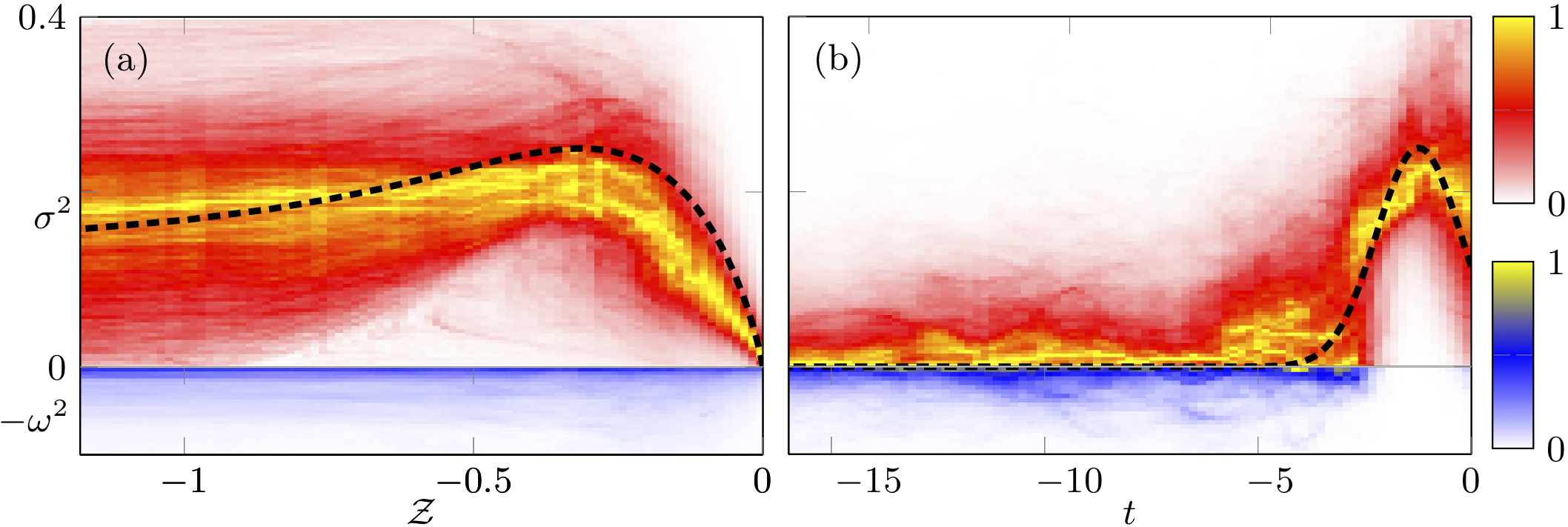
Figure 3: Optimal paths obtained from theory and path density for $\mbox{St}=0.31$ from DNS. (a) $(\mathcal{Z}_{\text{opt}},\sigma^{2}_{\text{opt}})$ from theory (dashed line). The colour-coded path density is the same as in Fig. 2(b). (b) $\sigma^{2}_{\text{opt}}(t)$ from theory (dashed line). The colour-coded path density is the same as in Fig. 2(c).

In order to explain these parts of our observations we need to go beyond the stability analysis, and consider how the fluid-velocity gradients reach the large threshold required to render particle neighbourhoods unstable. We do this in the following by computing their optimal fluctuation.

The steady-state correlation functions of $\mathbb{S}$ and $\mathbb{O}$, evaluated along particle trajectories in isotropic and homogeneous turbulence, have the general form

$$\langle S_{ik}(t)S_{jl}(t^{\prime})\rangle_{s} =C^{S}_{ijkl}\langle\mbox{Tr}\mathbb{S}(t)\mathbb{S}^{\sf T}\!(t^{\prime})\rangle_{s}\,,$$ (7a)

$$\langle O_{ik}(t)O_{jl}(t^{\prime})\rangle_{s} =C^{O}_{ijkl}\langle\mbox{Tr}\mathbb{O}(t)\mathbb{O}^{\sf T}\!(t^{\prime})\rangle_{s}\,,$$ (7b)

and $\langle S_{ik}(t)O_{jl}(t^{\prime})\rangle_{s}=0$. In two spatial dimensions, the tensors in Eqs. (7) are given by $C^{S}_{ijkl}=1/4(\delta_{ij}\delta_{kl}+\delta_{il}\delta_{jk}-\delta_{ik}\delta_{jl})$ and $C^{O}_{ijkl}=1/2(\delta_{ij}\delta_{kl}-\delta_{il}\delta_{jk})$. We express Eqs. (7) in terms of the basis (4) to obtain the steady-state correlations of $A^{i}$,

$$\langle A^{1}(t)A^{1}(t^{\prime})\rangle_{s} =\frac{1}{2}\langle\mbox{Tr}\mathbb{O}(t)\mathbb{O}^{\sf T}(t^{\prime})\rangle_{s}\,,$$ (8)

$$\langle A^{2}(t)A^{2}(t^{\prime})\rangle_{s} =\langle A^{3}(t)A^{3}(t^{\prime})\rangle_{s}=\frac{1}{4}\langle\mbox{Tr}\mathbb{S}(t)\mathbb{S}^{\sf T}(t^{\prime})\rangle_{s}\,.$$

All other correlations of $A^{i}$ are zero in the steady state. The right-hand sides of Eqs. (8) are parametrised as

$$\langle\mbox{Tr}\mathbb{S}(t)\mathbb{S}^{\sf T}(t^{\prime})\rangle_{s}=\mbox{St}^{2}C_{\text{S}}(\mbox{St})f[(t-t^{\prime})/s]\,,$$ (9a)

$$\langle\mbox{Tr}\mathbb{O}(t)\mathbb{O}^{\sf T}(t^{\prime})\rangle_{s}=\mbox{St}^{2}C_{\text{O}}(\mbox{St})g[(t-t^{\prime})/o]\,,$$ (9b)

with the non-dimensional correlation times $s$ and $o$ of $\mathbb{S}$ and $\mathbb{O}$, respectively. For tracer particles with $\mbox{St}=0$ one has $C_{\text{S}}(0)=C_{\text{O}}(0)=1/2$. Inertial particles with $\mbox{St}>0$ tend to avoid vortical regions due to preferential concentration [29, 30], so that $C_{\text{O}}(\mbox{St})<1/2$. The amplitude $C_{\text{S}}$, on the other hand, remains approximately equal to $1/2$ [26]. In our two-dimensional numerics, we also find $C_{\text{S}}(\mbox{St})\approx 1/2$ for Stokes numbers between $0.21$ and $0.51$. The functions $f$ and $g$ in Eqs. (9) are normalised to unity, $f(0)=g(0)=1$. Their time dependencies are well approximated by $f(t)=\exp(-t^{2})$ and $g(t)=\exp(-t)$ (see Fig. 1 in the SM [36]).

To describe how the fluid-velocity gradients reach the required threshold values, we model $A^{i}(t)$ as independent, stationary Gaussian processes with zero mean. For this class of processes, the most probable (optimal) fluctuation $A^{i}_{\text{opt}}(t)$ to reach a given threshold can be obtained by optimal-fluctuation methods, as we show in the SM [36]. By minimising the action associated with the path probability, we find that the optimal fluctuation of the fluid-velocity gradients is free of vorticity, $\omega^{2}_{\text{opt}}=0$, in agreement with our DNSs in Figs. 2(b) and (c). This result is intuitive: Vorticity contributes to $\mathcal{A}^{2}$ with a negative sign, so that any fluctuation of $\mathcal{A}^{2}=\sigma^{2}-\omega^{2}$ that reaches the large threshold $\mathcal{A}^{2}_{\text{th}}$ with finite vorticity requires an even larger strain contribution, to make up for vorticity. The optimal way to reach the threshold value is thus through paths that are vorticity free, whereas the probabilities of paths with finite vorticity are exponentially suppressed. The optimal path for the strain, by contrast, is found to be a time-localised fluctuation, $\sigma^{2}_{\text{opt}}=\mathcal{A}^{2}_{\text{th}}\text{e}^{-2(t-t_{\text{th}})^{2}/s^{2}}$, given by a Gaussian function peaked at time $t_{\text{th}}<0$ [36].

Using the optimal gradient fluctuation $(\sigma^{2}_{\text{opt}},\omega^{2}_{\text{opt}})$, we now obtain the explicit form for the optimal path $(\mathcal{Z}_{\text{opt}},\sigma^{2}_{\text{opt}})$ as a function of time. For $\mbox{St}\ll 1$, the left-hand sides of Eqs. (5) are small most of the time. To evaluate $\mathcal{Z}_{\text{opt}}$, we therefore use $A^{i}_{\text{opt}}$ as an input into Eq. (5). Making use of the fact that the vorticity is zero along the optimal path, $\omega_{\text{opt}}=0$, we find that $\mathbb{A}_{\text{opt}}=A_{\text{opt}}^{i}\mbox{\boldmath$e$}_{i}$ and $\mathbb{Z}_{\text{opt}}=1/2\mathcal{Z}_{\text{opt}}+z_{\text{opt}}^{i}\mbox{\boldmath$e$}_{i}$ can be brought into diagonal form by a Lorentz transformation [36]. The equations for the diagonal entries (eigenvalues) $\lambda^{\pm}_{\text{opt}}$ of $\mathbb{Z}_{\text{opt}}$ decouple into two equations,

$$\mbox{St}\tfrac{\text{d}}{\text{d}t}\lambda_{\text{opt}}^{\pm}=-\lambda_{\text{opt}}^{\pm}-(\lambda_{\text{opt}}^{\pm})^{2}\pm\frac{\mathcal{A}_{\text{th}}}{\sqrt{2}}\text{e}^{-(t-t_{\text{th}})^{2}/s^{2}}\,,$$ (10)

with initial conditions $\lambda^{\pm}(t_{0})=\pm\mathcal{A}_{\text{th}}\text{e}^{-(t_{0}-t_{\text{th}})^{2}/s^{2}}/\sqrt{2}$. The uncoupled Eqs. (10) are solved numerically, which yields the optimal path $\mathcal{Z}_{\text{opt}}$ using $\mathcal{Z}_{\text{opt}}=\lambda^{+}_{\text{opt}}+\lambda^{-}_{\text{opt}}$.

We note that for finite St, the threshold value $\mathcal{A}^{2}_{\text{th}}$, determined numerically [36], exceeds the value $1/8$ obtained from the stability analysis, in agreement with our DNS. The reason is that the optimal strain fluctuation $\sigma^{2}_{\text{opt}}(t)$ decreases for $t>t_{\text{th}}$. In order for $\mathcal{Z}_{\text{opt}}$ to reach negative infinity, $\sigma^{2}_{\text{opt}}(t)$ must exceed $1/8$ for a finite time so that $\mathcal{Z}_{\text{opt}}$ can become large and negative. The time for which the threshold must exceed $1/8$ decreases as St becomes smaller, and we recover $\mathcal{A}^{2}\to 1/8$ in the limit $\mbox{St}\to 0$.

In Fig. 3, we compare our theory and DNSs. The dashed line in Fig. 3(a) shows $(\mathcal{Z}_{\text{opt}},\sigma^{2}_{\text{opt}})$ obtained from Eqs. (10), with $\mbox{St}=0.31$ and dimensionless correlation time $s=2.1$ determined numerically. We observe qualitative agreement between the theoretically obtained optimal path and the (yellow) regions of high path density. However, Eqs. (10) slightly overestimate the threshold value $\mathcal{A}^{2}_{\text{th}}$. The likely reason is that the Stokes number in our DNS is too large to closely follow our analytical results, valid for $\mbox{St}\ll 1$.

Figure 3(b) shows the time dependence of $\sigma_{\text{opt}}^{2}(t)$ obtained from theory with $\mbox{St}=0.31$ (dashed line) and the corresponding path density from our DNS. We observe that the theory correctly predicts the localised, violent fluctuation of the strain prior to the formation of the caustic, which occurs at $t=0$. A considerable fraction of the large strain required to initialise the caustic persists at the time of caustic formation, which explains why caustics form preferentially in regions of large strain [26, 27]. For other Stokes numbers between $0.24$ and $0.51$, our DNS results lead to the same conclusion (data not shown).

In conclusion, we explained caustic formation in turbulent aerosols at small particle inertia as an optimal-fluctuation problem. In order for caustics to form, the fluid-velocity gradients must follow an optimal path, characterised by small vorticity and a violent strain that exceeds a large threshold. The remnants of the optimal fluctuation at the time of caustic formation result in a strong instantaneous correlation between large strains and caustic events.

Since caustics give rise to a multivalued particle-velocity field, and thus to high relative particle velocities, our results provide an explanation for the recently observed, instantaneous correlation between particle collisions and intense strain [26, 27]. The characteristic shape of the optimal path to caustic formation will allow one to identify caustics in experiments, and the strong instantaneous correlation of caustics and strain makes it possible to efficiently sample caustics in simulations.

The stability analysis described in this Letter can be generalised to three dimensions, where it reveals that particle neighbourhoods become unstable when the two invariants $Q=-\mbox{Tr}\mathbb{A}^{2}/2$ and $R=-\mbox{Tr}\mathbb{A}^{3}/3$ reach large thresholds in the $Q$-$R$ plane. We therefore speculate that optimal-fluctuation methods also explain caustic formation in three-dimensional turbulence at small Stokes numbers.