Artificial Neural Networks for Sensor Data Classification on Small Embedded Systems

Abstract

In this paper we investigate the usage of machine learning for interpreting measured sensor values in sensor modules. In particular we analyze the potential of artificial neural networks (ANNs) on low-cost microcontrollers with a few kilobytes of memory to semantically enrich data captured by sensors. The focus is on classifying temporal data series with a high level of reliability. Design and implementation of ANNs are analyzed considering Feed Forward Neural Networks (FFNNs) and Recurrent Neural Networks (RNNs). We validate the developed ANNs in a case study of optical hand gesture recognition on an 8-bit microcontroller. The best reliability was found for an FFNN with two layers and 1493 parameters requiring an execution time of 36 ms. We propose a workflow to develop ANNs for embedded devices.

Keywords Machine Learning, Artificial Neural Networks, Embedded Systems, Hand Gesture Recognition

1 Introduction

In automation and control systems, artificial neural networks (ANNs) are increasingly used to semantically enrich data recorded by low level sensors. Currently data recorded by sensors is digitized within the sensor modules and afterwards sent to a powerful infrastructure – nowadays often in a cloud – to perform the data enrichment with ANNs. However, for many standard tasks, capturing and digitizing the data together with the classification could be jointly implemented in sensor modules that are shipped for the usage in automation and control systems. This holistic type of in situ data processing would tremendously simplify the development of applications and would in many cases eliminate the need for an interface to a back-end system. A successful realization of this endeavor would in addition reduce the time until the interpretation of the data is available. Higher abstractions of the sensed data can simply be queried from the sensor module via a digital interface.

This paper investigates, how ANNs can be used within sensor modules equipped with a low-cost microcontroller for the enrichment of data captured by sensors. The focus is on temporal data series. We analyze how an ANN must be designed and implemented in order to execute it on a low-end microcontroller with a few kilobytes (kB) of RAM and flash memory only. The challenge is that microcontrollers in off the shelf sensor modules only have a tiny fraction of the computational power of a high-performance computer or cloud infrastructure. Especially in low-cost sensor modules built-in microcontrollers are often 8-bit controllers. The software for sampling and conversion already requires a part of the available RAM and flash memory limiting the leeway for an additional application. The goal of this work is to develop ANNs that provide a high level of reliability for the recognition and classification of time series of sensor values within the memory and processing limits of a standard microcontrollers.

In Sec. 2 the general use of ANNs on microcontrollers is reviewed with a focus on sensor modules. Sec. 3 presents the case study used in this work, a sensor module for the optical recognition of hand gestures. In this section we also discuss architectural options for ANNs classifying series of images as gestures. The validation of the proposed architectures is presented in Sec. 4. The following section provides general recommendations for employing ANNs in sensor modules, before Sec. 6 concludes the paper.

2 ANNs in Sensor Modules

The primary use of ANNs in sensor modules is to semantically enrich data measured by its sensors. ANNs can detect events or states, which can only be inferred from sequences or combinations of values measured by several sensors. Thus, an ANN can undertake the non-trivial task of classifying sensor values and mapping them to classes. For this task, the ANN has to be trained. This usually requires training data consisting of measured sensor data and its attribution to classes. The computationally intensive training phase is typically not executed on the sensor module but on high-performance computers and is therefore not constricted by the resources of the sensor module. The resulting trained model can be installed on sensor modules within a product. Thus, the ANN has to get along with two limitations: The executable code and the run-time memory requirements for static variables and stack have to fit into the microcontroller’s storage systems and the execution time of the code must be within the limits predetermined an application.

2.1 State of the Art Machine Learning in Sensor Modules

The use of ANNs and other types of machine learning (ML) to semantically enrich sensor data is not a new approach. However, in most cases, values acquired by sensors are sent to powerful computing devices for semantic enrichment such as cloud servers. One of the many applications found in literature is the sensor-based recognition of human activities from sensor values [30]. Another application is health monitoring of machines, where the wear level is determined from sensor data obtained directly from or in the vicinity of the machines [32]. Saleh et al. used ANNs to classify the behavior of car drivers into aggressive, normal, or drowsy based on data from a GPS module, an accelerometer, and a video camera [27]. Wang, Yu, and Mao determine the position of smartphones from the progression of the values of its magnetic and light sensors [31]. Already in 1998, Holmberg et al. published their work on determining the type of bacteria growing in petri dishes using an ANN classifying values from an electronic nose with 15 gas sensors [10].

Jantscher favors executing artificial intelligence (AI) in sensor modules instead of transmitting sensed data to powerful computing devices. The main advantage is a significant reduction of the latency between data acquisition and the reaction of a system. The approach also reduces the amount of data transmitted in networks and the load on servers. The reduction of network traffic also leads to lower energy consumption. The local processing will allow more complex sensor systems in the future. Jantscher developed a sensor module with several metal-oxide (MOX) based gas sensors. Their resistance changes for different gases. He trained an ANN to determine the type of gas from the progression of resistance values of the MOX gas sensors [13].

Pardo et al. use an ANN that is trained and executed on a sensor module to forecast time-series of indoor temperatures from values measured in the past. The sensor module contains an 8-bit microcontroller Texas Instruments CC1110F32 with 4 kB of RAM and 32 kB of flash memory, and an integrated radio transceiver for wireless communication. The training of the ANN was performed on the fly and in situ, i.e., it was based on measured sensor values that were not stored for longer times [19].

Leech et al. implemented sensor modules to determine the room occupancy with a single PIR-Sensor. They used Bayesian networks – a well-known ML technique. The network is initially trained on a powerful computer. Afterwards the training is continued on the sensor module. They compare implementations for two microcontrollers, an Arm Cortex-M4F with a floating-point unit (FPU) and an Arm Cortex-M0 without. An FPU is a circuit performing floating-point operations in hardware. Without an FPU, a compiler has to translate floating-point operations into sequences of integer operations at the cost of increased computation time. The Cortex-M4F has 96 kB RAM, 512 kB flash memory, and a clock rate of 84 MHz. The Cortex-M0 has 12 kB RAM, 128 kB flash memory, and a clock rate of 48 MHz. Using the Cortex M4F increased the execution speed by a factor 2.3 without using the FPU compared to Cortex M0. This can partly be explained by the higher clock rate. Using the FPU increased the execution speed by another factor 8.3. The total speedup of 19 comes at the cost of an increased power consumption of a factor 2.5 [15].

Suresh et al. use a wireless, battery operated sensor module to classify the activities of animals based on values of an accelerometer. They apply the k-nearest neighbors technique (kNN). For each classification of an activity, 64 sensor values are used to calculate statistical values, such as mean, co-variance, wavelets, and moments. These are the inputs for the kNN algorithm classifying the activity. An Arm Cortex-M0 is used for execution. The classification reduces the data to be sent over the wireless radio by a factor 512 compared to the raw data. This significantly extends the battery life time [28]. Patil et al. use a wireless sensor module with ML as part of a human machine interface for blind people to control their smart phones. The sensor module with accelerometer and gyroscope is attached to their white cane. It detects gestures such as a double tap on the ground as well as rotary and swivel movements. Gestures are sent to the smartphone via Bluetooth. The classification is performed with a kNN algorithm. Data collection, preprocessing and classification takes 63 ms on an Arm Cortex-M0 with 32 kB RAM, 256 kB flash memory, and a clock rate of 48 MHz [20].

A product of Bosch is a motion detector sensor module for a wireless intrusion alarm system. It uses AI to only react on humans but not on pets. For this purpose, it has passive infrared and microwave Doppler radar sensors. It is not further specified which type of AI is used [29]. Sony recently started offering a vision sensor module with an integrated digital signal processor (DSP) for AI processing. It consists of two stacked chips, an image sensor with 12.3 megapixels and the DSP for AI behind it. The DSP can be programmed for different types of AI such as ANNs. It is meant to process AI models in real-time at a rate of 30 images per second. Sony sees applications such as real-time object tracking, counting customers, or detecting stock shortages in super market shelves [23].

ML can be implemented for small microcontrollers of sensor modules by manually writing the code, or with libraries or compilers created for this purpose. Lai, Suda, and Chandra developed a library for executing ANNs on 32-bit Arm Cortex M microcontrollers having the Multiply-and-Accumulate instruction (Cortex M3, M4, and M7). The library provides functions to efficiently implement the calculations needed for ANNs [14]. In contrast, Gopinath et al. developed the domain specific language SeeDot for describing the matrix operations needed for ML, and a compiler generating efficient C code for microcontrollers from that. They focus on microcontrollers with few kB of RAM and without FPU, experimenting with Arduino Boards (with Microcontrollers ATmega328P and ARM Cortex M0), and FPGAs [6].

2.2 ANNs on Small Microcontrollers

In principle, small microcontrollers can perform all types of calculations including the execution of ANNs. However, their small memory only allows programs with a small footprint. Furthermore, many microcontrollers do not have an FPU. Floating-point operations, commonly used for ANNs, thus entail a large number of integer operations decreasing performance. Nevertheless, specially designed and tuned ANNs can still be executed on microcontrollers.

An ANN can be seen a universal function (Feed Forward Neural Network) or an automaton (Recurrent Neural Network) whose behavior is customized by selecting a network structure (architecture) and appropriate configuration parameters. The architecture is selected by developers and defines the general abilities of the ANN. Parameters are selected in the training phase when parameters are adjusted by optimization algorithms. For a set of desired input-output pairs (training data), parameters are updated to make the ANN produce values close to the outputs for the given inputs. ANNs then typically generalize the desired behavior to other inputs. More detailed introductions to ANNs can be found in literature [18, 5]. In the following we describe the variants of ANNs that we use in our work and discuss their suitability for usage in embedded systems.

2.2.1 Feed Forward Neural Networks (FFNNs)

An FFNN approximating a function is an acyclic directed graph connecting processing elements called neurons. A simple example is illustrated in Fig. 1. Neurons (illustrated as circles) are commonly organized in layers. The neurons of a layer get their inputs from the output of the neurons of the previous layer. In the common case of fully connected (dense) layers, the results of each neuron of a layer are given to each neuron of the following layer. Neurons of the so-called output layer produce the outputs, i.e., the results of the FFNN. Other layers are called hidden layers. The FFNN in Figure 1 has a single hidden layer. Inputs to the FFNN are provided to the first hidden layer via an input layer. Each input value is also called a feature (illustrated as a square). The aggregate of the number of layers, the number of neurons per layer, its features and the connections between neurons is called the architecture of an ANN.

Figure 1: Example of an FFNN architecture

The transformation of the input to the output of a neuron is illustrated in Fig. 2. Each input $x_{i}$ is multiplied with a weight $w_{i}$. The results are summed up together with the bias $b$. The sum is given to a so-called activation function that calculates the result of the neuron, called its activation. Common activation functions are discussed in Sec. 2.2.3. Weights and bias values are the parameters selected during training to approximate the desired function. For the ANNs considered in this paper, biases can vary for each neuron and weights can be different for each input of each neuron. The weights of all neurons of a layer as well as its inputs and outputs are often represented as a matrix. This allows to interpret the sum and the multiplications as a matrix multiplication. The aggregate of all weights and biases of an ANN, together with its architecture, is called a model. It determines the function computed by the FFNN.

Figure 2: Transformation of the inputs of a neuron to its output

In a sensor module, the ANN calculates classes as outputs from features derived from measured sensor values. Sensor values measured by analog-digital converters (ADC) are commonly pre-processed. At least, each value is normalized to the interval $[0;1]$ or $[-1;1]$. For classifications, each neuron of the output layer represents a class to be detected. In the ideal case only one neuron has an activation significantly larger than zero indicating the detection of this class. If an application allows that no class is detected, an additional neuron can be added to signal this case.

The computational effort for executing an FFNN can be roughly assessed with the number of multiplications or the number of additions respectively. Both numbers equal the number of weights, as each weight is multiplied once and added. The number of multiplications can be calculated from the network structure by counting the edges. It is the number of edges between two neighboring layers, which is the product the neurons (or features) of both layers. For the FFNN in Fig. 1, there are 9 edges between the 3 features of the input layer and the 3 neurons of the hidden layer. In addition, there are 6 edges between the 3 neurons of the hidden layer and the 2 neurons of the output layer. In total the FFNN has 15 edges and weights, and requires 15 multiplications to execute it. For a more accurate modeling of the computation effort, the number and type of activation functions once evaluated per neuron must be considered (see Sec. 2.2.3). The memory required to store the non-optimized model is proportional to the number of parameters. It is thus the number of weights as calculated in the previous paragraph plus the number of biases. The number of biases is the number of neurons in the ANN, as every neuron has a bias. The example from Fig. 1 has 5 neurons and biases. With the 15 weights it has 20 parameters in total.

Figure 3: Example of an RNN architecture

2.2.2 Recurrent Neural Networks (RNN)

An RNN implements a universal automaton having a state, whose behavior can be trained. It is a graph of neurons having cycles. Cycles are commonly found within layers, providing the outputs of each neuron as additional inputs (feedback) to all neurons of the same layer, as illustrated in Fig. 3 for the hidden layer. Layers with cycles are called recurrent layers. The feedback gives an RNN a state. Thus, the output of an RNN can be different for the same inputs. For this reason, an RNN can process sequences of features, storing parts of it in its state. It can also output sequences of values for fixed sets of features.

In a sensor module, an RNN can be used to classify sequences of sensor values. Features are produced from sensor values as for FFNNs. However, the state of the recurrent layers allows remembering conditions from previous execution steps, that is, from previously measured values. A class, signaled as an activation of an output layer neuron, can thus depend on sensor values of different execution steps.

As for FFNNs, the computational effort for executing one step of an RNN can be roughly assessed with the number of required multiplications, which equals the number of weights. For a recurrent layer, it is the sum of the number of edges in the graph between each neuron and the neurons of the same and the neighboring layer. Thus, if a layer with n neurons receives its inputs from a neighboring layer with m neurons then there are $(n+m)*n$ edges. In the example in Fig. 3, there are thus 18 edges for the $m=3$ features and the $n=3$ neurons of the recurrent hidden layer. Six additional edges exist between the neurons of the hidden and the output layer. In total the RNN has 24 edges and weights, and requires the same number of multiplications for execution. The memory for storing the model of an RNN is again assessed by the number of parameters, i.e., its weights plus its biases. The RNN in Fig. 3 has 29 parameters, 24 weights and 5 biases for its 5 neurons.

Long Short-Term Memory (LSTM) networks [9] are not considered in this paper to minimize the requirements for memory and execution time. LSTMs are the RNNs generally found in current literature (e.g. [32, 27, 31, 4, 33]) as they solve the vanishing gradient problem for training RNNs [8]. However, compared to RNNs containing simple neurons described above, LSTM networks require about four times as many parameters and also the effort for the execution is about four times higher. This makes them unsuitable for small microcontrollers.

2.2.3 Activation Functions

A significant portion of the ANN’s execution time is needed for evaluating activation functions in addition to multiplications and additions. Activation functions have to be evaluated once for each neuron. They need to be differentiable to enable the so-called back-propagation required for training [18]. Commonly used activation functions have significantly different evaluation times. However, the selection of a function can also influence the accuracy of the classification. Ertam and Aidin give a list of common activation functions [3]. Usually the same activation function is used for all neurons of a layer. Tab. 1 lists the activation functions considered for this paper. The two functions traditionally used are Sigmoid and Tanh. Both are smoothed versions of a step function changing its output value at zero [18]. However, while Sigmoid changes its output from 0 to 1, Tanh changes from -1 to 1. One of the two functions is thus selected depending on the desired output range.

Table 1: Activation functions used in this paper

Name	Function	Plot	Evaluation time on ATmega328P
Sigmoid	$f(x)=\frac{1}{1+e^{-x}}$		$170\mu$s
Tanh	$f(x)=\frac{1}{1+e^{-2x}}-1$		$\approx 170\mu$s
Hard Sigmoid	$f(x)=\begin{cases}0&\text{if }x<-2.5\\ 1&\text{if }x>2.5\\ 0.2x+0.5&\text{otherwise}\end{cases}$		$15\mu s$
Softsign	$f(x)=\frac{x}{1+|x|}$		$41\mu s$
Relu	$f(x)=\begin{cases}x&\text{if }x\geq 0\\ 0&\text{otherwise}\end{cases}$		$5\mu s$
Softmax	$f(x_{i},\vec{x})=\frac{e^{x_{i}}}{\sum e^{x_{i}}}$	$\begin{cases}\vec{x}&\text{All activations of a layer}\\ x_{i}&\text{Activation of }i^{th}\text{ neuron}\end{cases}$	$\approx 170\mu s$ per neuron
Max	$f(x_{i},\vec{x})=\begin{cases}1&\text{if }x_{i}=\max(\vec{x})\\ 0&\text{otherwise}\end{cases}$		$5\mu s$ per neuron

For microcontrollers, the major disadvantage of Sigmoid and Tanh is the computational effort required to evaluate the exponential function. Hard Sigmoid and Softsign were developed to approximate these functions with a low evaluation effort. Hard Sigmoid approximates Sigmoid by a linear function for inputs around 0 with a minimum output value of 0 and a maximum of 1. Softsign approximates Tanh using a division, addition, and an absolute value. Rectified Linear Units (Relu) is a linear function clipped to zero for negative values [17]. This can be implemented efficiently with a conditional statement.

Softmax is frequently applied in the output layers of classifications. It differs from the above activation functions in that it can only be calculated for an entire layer. It normalizes the activations of the neurons to values between 0 and 1, with the sum of all activations being 1. Therefore, the activation of a neuron can be interpreted as the probability that the features imply the corresponding class. For microcontrollers, there is again the disadvantage, that an exponential function has to be executed for each neuron.

Softmax can be replaced for execution with Max, if an application only requires finding the largest activation of a layer with Softmax. Max returns 1 for the largest activation and 0 for all others. This can be calculated efficiently with one numeric comparison per neuron. Softmax must still be used for training, as Max is not differentiable. Max cannot be used for recurrent layers, as its activations used as inputs for the same layer are significantly different from the values of Softmax used for training.

2.2.4 Use-Case: Microcontroller ATmega328P

In this work we utilize the microcontroller Atmel ATmega328P [2] as use-case to discuss its ability to execute ANNs. It is a low-cost, 8-bit microcontroller often used in sensor modules. This microcontroller is found on Arduino Uno boards [1]. The RISC processor with Harvard architecture runs at up to 16 MHz with most instructions requiring only a single clock cycle for execution. It provides 2 kB of RAM and 32 kB of flash memory for programs and static data but no hardware FPU for floating-point operations.

The ATmega328P has no memory cache. This is typical for small microcontrollers to simplify their circuits. It is therefore assumed for all discussions in this paper. If a cache would be available, the order of memory accesses had to be considered to reduce the execution time of ANNs.

The maximum size of an ANN to be stored in a sensor module is limited by the flash memory of its microcontroller. After training, the parameters are compiled and linked with the program, and uploaded to flash memory. Microcontrollers have instructions to directly read data from that memory during computations. The obvious, naïve approach is storing parameters as float values requiring 4 bytes per value. The 32 kB of flash memory of the ATmega328P would then allow storing up to 8192 parameters. Up to 16384 parameters are possible when storing each parameter in 2 bytes or 32768 parameters stored in a single byte. Fixed-point number formats could be used for that purpose. However, the maximum numbers of parameters can only be considered as an upper bound, as a part of the flash memory is needed for the program controlling the sensor module.

The size of the RAM restricts the possible number of neurons per layer. The execution of a layer requires variables for all its inputs and activations. Further variables for intermediate values can be reused as each neuron is calculated individually. The activation functions Softmax and Max are an exception, as the results of the exponential function (Softmax) or the sum (Max) are needed from all neurons, before the final activations can be calculated. However, the variables of the inputs can be reused to store the final activations. The number of variables needed to process a non-recurrent layer is thus the sum of the number its neurons plus the neurons (or features) of the previous layer. If the current layer has more neurons and Softmax or Max is used, it is twice the number of neurons of the layer. For recurrent layers it is twice the number of its neurons plus the neurons of the previous layer or three times the neurons of the layer itself if greater for Softmax or Max. The variables needed for an ANN is the maximum needed for one of its layers.

Only a part of the RAM can be used for inputs and outputs of layers, as RAM is also necessary of other purposes including the stack. Assuming that half of the RAM is used for this purpose and float variables require 4 bytes, the ATmega328P enables the use of 256 variables requiring one kB. This can be used for non-recurrent layers of $256/2=128$ neurons or recurrent layers with $256/3\approx 85$ neurons, provided all layers have the same number of neurons. Slightly bigger numbers are possible for a non-recurrent layer, if both neighboring layers are smaller. Large numbers of f features require a smaller first layer having less than 256-f neurons, also restricting the number of features to less than 256.

The ATmega328P needs about 18 $\mu$s to multiply a weight with its input value and add the result to the sum assuming calculations with 4-bytes float values. This was measured with an RNN having 631 weights for 3 layers requiring an execution time of 11.36 ms. Evaluation times for activation functions were subtracted.

Measured times for evaluating activation functions on ATmega328P were given in Tab.1. The evaluation of Sigmoid requires 170 $\mu$s. Of this, the evaluation of its exponential function requires 162 $\mu$s. Tanh is estimated to have a similar evaluation time, as it requires similar calculations as for Sigmoid. Softsign, the approximation of Tanh, requires 41 $\mu$s. That is nearly three times as much as the 15 $\mu$s needed for Hard Sigmoid, the clipped linear approximation of Sigmoid. As expected, the lowest evaluation time was measured for Relu only requiring 5 $\mu$s. The evaluation time of Softmax and Max depends on the number of neurons of the entire layer. Experiments showed an evaluation time of 170 $\mu$s per neuron, which is the same as for Sigmoid. As expected, Max has a very short evaluation time of 5 $\mu$s per neuron.

The evaluation times of Softmax, Sigmoid and Tanh can be significantly reduced, with a fast approximation of the exponential function. The approximation needs to be differentiable to be usable during training, but the accuracy is of minor importance. A suitable approximation was developed based on the observation that $2^{x}$ can be efficiently calculated on microcontrollers if x is an integer by adding $x$ to the exponent of a float number or by bit-shifting in fixed-point numbers. For non-integers, $2^{x}$ can be interpolated between adjacent integers. The quadratic approximation given in (1) is differentiable, as its derivative is continuous. It can be used for an approximation of the exponential function with (2).

$$2^{x}\approx 2^{n}\left(1+\frac{2}{3}v+\frac{1}{3}v^{2}\right)\text{ with }n=\lfloor x\rfloor\text{ and }v=x-n$$ (1)

$$e^{x}=2^{\frac{x}{\ln 2}}$$ (2)

Measurements show that the approximation of the exponential function can be evaluated by the ATmega328P in about 75 µs. This is less than half of the 162 µs required for the accurate implementation. The maximum relative error of the approximation is less than 0.5%. The approximation was used to implement an approximated Softmax. This required an evaluation time of 83 µs per neuron. Sigmoid and Tanh are expected to require similar evaluation times.

Tab. 2 shows execution times of an RNN with 631 weights. The RNN processes 12 features with 2 hidden layers and an output layer. Each non-recurrent hidden layer had 9 neurons. The output layer with 17 neurons was recurrent. Four different activation functions were tested for the two hidden layers. Softmax, Max, and the approximated Softmax were applied for the output layer. The measurements show, that the activation function can require up to one third of the execution time of the ANN if Sigmoid and Softmax is used. On the other hand, the evaluation time of activation functions is negligible if Relu and Max is used instead.

Table 2: Execution time of ANN with 631 weights on ATmega328P

Activation functions used	Evaluation time for activation functions	Total execution time of ANN
Sigmoid – Sigmoid – Softmax	5.95 ms	17.31 ms
Hard Sigmoid – Hard Sigmoid – Softmax	3.16 ms	14.52 ms
Softsign – Softsign – Softmax	3.63 ms	14.99 ms
Relu – Relu – Softmax	2.98 ms	14.34 ms
Relu – Relu – Max	0.18 ms	11.54 ms
Relu – Relu – Approximated Softmax	1.50 ms	12.86 ms

An upper bound of the execution time of an ANN on the ATmega328P can be estimated from the number of parameters, that can be stored. As discussed above, at most 8192 (resp. 32768) parameters can be stored in flash memory as 4-byte (resp. 1-byte) float values. A major share of the execution time is determined by the number or multiplications and additions that equals to the number of weights. The number of weights is the major share of the parameters, as each neuron has several inputs and their weights, but only one bias. Hence, an ANN on the ATmega328P is restricted to 8192 multiplications and additions requiring 18 µs each, or 32768 multiplications for 1-byte parameters. The limit for the execution time for multiplications and additions is thus 147 ms resp. 590 ms for 1-byte parameters. In addition, the evaluation of activation functions requires at most about half of that. Note that this discussion assumed that each weight is stored in flash memory individually, which is not the case for compressed ANNs discussed in the next subsection.

In summary, the ATmega328P is able to execute ANNs with up to about 6000 parameters (significantly less than 8192) having up to 128 neurons per non-recurrent or 85 neurons per recurrent layer and less than 256 features. This assumes the use of 4 bytes float values without compression. The execution time depends on the number of weights and the activation functions used and is less than 150 ms.

2.2.5 Compression of ANNs

Han, Mao and Dally introduced deep compression to address the memory and performance limitations of embedded systems for executing ANNs [7]. They propose a three-step process consisting of pruning of irrelevant edges, trained quantization to enable many edges to share one stored weight value, and Huffman coding for further memory reduction. Their work considers embedded systems such as mobile phones, which are significantly more powerful than the modules considered in this paper. They compress the AlexNet Caffemodel with 61 million weights from 240 megabytes (MB) to 6.9 MB and the VGG-16 Caffemodel with 138 million weights from 552 MB to 11.3 MB with no loss of classification accuracy.

Pruning is applied to a trained ANN by setting those weights to zero that are almost zero. It is assumed that the corresponding edges have no significant influence on the accuracy of the ANN. Setting a weight to zero eliminates the associated edge eliminating the associated multiplication and addition. Afterwards the remaining weights are fine-tuned by retraining. Pruning removed 89% of the edges for AlexNet and 92.5% for the larger VGG-16.

Quantization is implemented with k-means clustering [16] applied individually for each layer. All weights of a layer are classified into $k$ clusters. The centroids of the clusters are used as the desired $k$ shared weights replacing all weights falling into a cluster. Again, retraining is applied for fine-tuning. The training is modified to change the shared weights of the clusters instead of the individual weights.

To save memory for storing a quantized model, each weight of an edge is stored as an index to a table containing the shared weights. For $k$ shared weights, an index only requires $\lceil\log_{2}k\rceil$ bits. For AlexNet and VGG-16, 256 or 32 shared weights were used depending on the layer, requiring 8 or 5 bits to encode weights. This compressed the model size to 3.7% or 3.2% respectively, compared to storing each weight in 4 bytes. Further size reduction is enabled by compressing the resulting model with the lossless Huffman code [11]. This compressed the model size of AlexNet to 2.88% and 2.05% for VGG 16. Deep compression can also speed up the execution of an ANN. Han et al. analyzed this for individual layers of AlexNet and VGG-16 for pruning only [7]. For three layers of AlexNet, a speedup between 1 (no speedup) and 5 was observed on an Intel Core i7 5930K CPU. For the layers of VGG-16 the speedup was between 1 and 10.

Roth et al. survey the more recent state of the art to increase the execution efficiency of ANNs for embedded systems [25]. They look at the combinable approaches also used by Han et al.: pruning, quantization, and efficient encoding of models, but also on how to find a resource-efficient architecture. Again, the view is on processors that are more powerful than those considered in this paper.

Pruning techniques are divided into unstructured and structured pruning. The unstructured pruning, setting individual weights to zero, was discussed above. It can be improved if pruning becomes reversible, restoring a pruned weight if the retraining reveals that it is useful. This increased the number of edges pruned from AlexNet to 94% with no loss of accuracy. Structured pruning sets groups of weights to zero that represent all inputs of a neuron or all inputs using the activation of a neuron or feature, or the same for sets of neurons. This is desirable, as it allows removing entire neurons or features from the ANN. However, it is more sensitive to loss of accuracy than unstructured pruning. Finally, with dynamic network pruning, parts of an ANN are not always executed during runtime. Another ANN or a part of the same decides about the execution.

Many approaches of quantization share the idea of reducing the number of bits for storing weights as well as for storing activations. Fewer bits for weights reduce the size of the model and fewer bits for activations reduce the RAM required for execution. Besides the table approach described above, floating-point and fixed-point formats with different bit width are an option as well as storing values of the power of two only, binary values (e.g. -1, 1), or ternary values (e.g. -1, 0, 1). This can also increase the execution speed, as integer operations or binary logic are faster than floating-point operations. Quantization can be performed after or during training. To quantize during training, weights are stored for the training process as full-precision values. Quantization is performed on demand, when the ANN is executed for a record of the training data (forward propagation). However, gradients for improving the weights are calculated and applied to the weights in full-precision bypassing the quantization.

Three basic approaches are given to find resource-efficient models or architectures for ANNs. With knowledge distillation, training data is used to train a large ANN first. Afterwards a smaller ANN is trained from training data produced with the large ANN. This results in a small ANN achieving a better accuracy than a small ANN trained with the original training data. A suitable architecture for an ANN can be developed with manual design using common design principles and building blocks. Alternatively, neural architecture search allows automatically searching a suitable architecture from a discrete space of possible architectures.

The approaches for compression can also be applied to ANNs used in sensor modules. However, their impact on memory requirements and execution times are difficult to state in general terms as it is application specific. Pruning removes those features, neurons, or edges of a dense layer that are not necessary to implement the specific function required by the application. Quantization reduces the variety of weights to the amount required by that function or to the accuracy level still sufficient for the application. The impact on memory requirements and execution time for a specific application is discussed in Sec. 4.4.

2.3 Choosing an ANN Architecture for a Sensor Module

The ANN architecture to be used in a sensor module depends on the classification problem at hand. If the classes are determined based on values, measured with one or several sensors at the same time, an FFNN is an obvious choice with the (normalized) sensor values as inputs and the classes as outputs. If classes are determined by the changes of measured values, FFNNs can be used by providing the gradients as inputs or by providing two successively measured values of each sensor. If a fixed number of successively measured values determines a class, all these values can be given to an FFNN requiring many features that increase the memory and computation effort.

If a class is determined by a non-fixed number of successively measured values, then RNNs are a natural choice. A simple example is a sensor module for decoding characters in Morse code with a sensor measuring the noise level or brightness to determine the characters (classes) sent at different speeds. After each measurement, the (normalized) sensor value is processed by the RNN. The RNN is trained to store the state required to detect the classes from these sequences. This allows recognizing the class in retrospect.

However, FFNNs can also be applied for classifying sequences with non-fixed numbers of successively measured values, provided the values are stored in a ring buffer large enough for all successive sensor values that determine a class. After each measurement, the FFNN is executed with the entire buffer as input, returning a class. The FFNN must be trained to avoid misclassification due to the same sensor values given to the FFNN several times in different locations of the buffer after successive measurements.

If the start and end of the sequence of sensor values determining a class can be detected, the sequence can be buffered and given to the FFNN for classification. This requires finding an algorithm to detect these two events. The approach requires less computing effort, as the ANN is only executed once after the end of the sequence. The classification of the ANN can be simplified, if the non-fixed number of sensor values can be normalized to a fixed number having relevant features determining a class at fixed inputs of the ANN.

3 Case Study: Optical Recognition of Hand Gestures

A hand gesture sensor module is used as a case study for this paper. It recognizes a set of hand or arm movements and signals these gestures via a digital interface. The target of our research are low end microcontrollers, driven by the main constraint for this study: low costs. The aim is a final price of a sensor module below 1 Euro in mass production. An array of 3x3 or 4x4 light sensors is applied as camera. An off the shelve microcontroller reads light sensor values (light values) and executes an ANN to classify sequences of light values, therefore recognizing the gestures. For simple devices, the microcontroller can be programmed to control the entire device.

The sensor modules can be used for many applications where devices require a contactless handling. It may be applied for devices in sterile environments (such as operating rooms) to avoid contamination by or of the hands of a surgeon. It allows controlling automation processes or devices in the industry if workers carry tools in their hands, wear thick gloves, or have extremely dirty hands. Public information displays that are entirely protected behind glass can still be operated by passers-by.

3.1 Hand Gestures

A hand gesture sensor module is trained to recognize a fixed set of gestures, called its gesture set. The gestures to be used depend on the device to be controlled. The selected gesture set must be sufficient to control the device and reliable identification each gesture must be guaranteed.

Preim and Dachselt summarize non-technical recommendations and challenges on gestures [22]. Users must be able to perform gestures quickly and with little effort. Gestures have to be natural and easy to learn, such as a simple wipe from left to right. The gestures set should be small to firstly ensure that users quickly learn them and secondly to enable a fast and reliable recognition. Movements in opposite directions should be used for opposite commands (e.g. on and off). Gestures have to be socially acceptable, especially in the public (e.g. no excessive, unnatural movements). The beginning and ending of a gesture must be detectable from the continuous stream of sensor values. The recognition process must provide a high degree of tolerance such that variations in the applications by different users and even by the same do not lower the recognition rate. Users have to be informed about the recognition or failure during or immediately after the gesture.

Gestures can be static or dynamic, and discrete or continuous. In a static gesture a statement is represented as a static pose (e.g. a fist), while dynamic gestures represent statements as movements (e.g. wipe of a hand) [22]. A gesture is called discrete, if it is discretely recognizable and triggers a command after its completion. It is dynamic if it is continuously recognizable and can continuously trigger commands.

For sensor modules, where gestures are to be recognized from videos with 3x3 or 4x4 pixels, static gestures are not applicable. The low resolution only allows recognizing movements, but not individual pictures with poses. In general, discrete and continuous gestures are feasible. However, the gesture set used for this study illustrated in Tab. 3 only contains four discrete gestures, each consisting of a complete movement of the hand over the sensor module: From left to right, right to left, from top to bottom, and bottom to top.

Table 3: Gesture set analyzed in this paper

Gesture Set used
Interpretation for menu in Sec. 3.2	Forward	Backward	Select	Abort

3.2 Sample Application: Controlling a Fully Automatic Coffee Machine

The developed gesture recognition was used to control the fully automatic coffee machine Jura Impressa S9 to brew different types of coffee and configure the machine. This was implemented with the sensor module and the ANNs described in section 4. The sensor module is connected to the service interface (UART) of the coffee machine. It allows to trigger the brewing of different types coffee, writing on the display (2 x 8 characters), and querying and changing state and settings of the machine. The interface provides a voltage line that is used to power the sensor module.

A multilevel menu that is not provided by the coffee machine was implemented in the sensor module. It can be adapted to other device types with little effort. The menu state is stored in variables of the microcontroller and written to the coffee machine’s display via the interface. The multilevel menu is controlled with the gesture set from in Tab. 3. It starts at the top-level menu providing options for brewing different types of coffee, to change settings, and to turn the machine off. Two gestures (Forward and Backward) are used to switch forth and back between these options. A third gesture (select) allows selecting an option, which starts brewing, saves a setting, or leads to a sub-menu. If the settings option is selected from the top-level menu, a sub-menu is entered that allows changing the quantity of coffee used in a brew process. The type of coffee for which this quantity is applied is selected first. A further sub-menu allows selecting eight options of possible quantities. Each menu can be left to its parent menu with a fourth gesture (abort). The hierarchy of the menus can be extended for further functionality.

3.3 ANNs for Hand Gesture Recognition

In order to recognize hand gestures with an ANN, temporal sequences of light values need to be classified into gestures. A gesture is detected after its completion. Each light sensor measures the light value of one pixel. The values of all light sensors are measured simultaneously leading to an image. For gesture detection, an image allows determining the hand’s position before the sensor module. The gesture is finally inferred from a sequence of images showing the movement of the hand. Fig. 4 depicts an example of seven selected images of a hand gesture from left to right captured with our sensor module.

Figure 4: Selected images of a hand gesture from left to right

The number of images constituting a gesture depends on the speed of the hand movement. As discussed in Sec. 2.3, an RNN or an FFNN with a buffer are suitable network structures for this kind of classification problem. Gestures constitute the classes to be recognized. However, it is also possible to recognize parts (phases) of gestures to determine complete gestures in a post-processing step. Three approaches are discussed and validated in more detail below.

3.3.1 RNNs Recognizing Gestures

A straightforward approach for recognizing gestures are RNNs with gestures as classes. The normalized light values of each image measured at the same time, are given to the RNN as features. The network maintains the state while transitioning from one image to the next. It signals the detection of a gesture with the activation of an output neuron after the gesture is completed.

The RNN architecture used for this study is illustrated in Fig. 5. The output layer has 5 neurons and uses the activation function Softmax. Four of them represent the gestures to be recognized. The fifth is used to indicate that no gesture was recognized. With Softmax, each activation of the output layer can be interpreted as the probability that one of the gestures or no gesture was recognized. For efficiency reasons Max can replace the activation function Softmax after training. The RNN should have at least one hidden layer and one of them needs to be recurrent to retain the state between images. Images are given to the first hidden layer as features. The microcontroller ATmega328P discussed in Sec 2.2.4 has 10-bit analog digital converters. The resulting light values are in the interval $[0,1023]$. To use them as features they are normalized to the interval $[0,1[$ by a division.

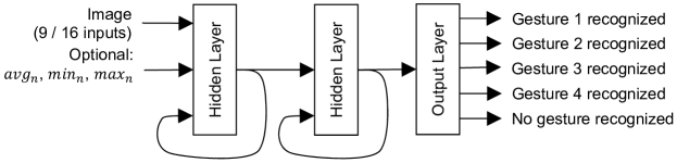
Figure 5: RNN for recognizing gestures

In addition to the light values, further features can be pre-calculated from that. Three candidates are a rolling average, minimum, and maximum providing information about the brightness of the hand and the environment. The RNN can use this to simplify abstracting from the ambient brightness and the type of illumination. The three values are continuously calculated. Therefore, only a single variable is necessary that is updated once for every light value $s_{n,i}$ at time step n with equations (3), (4), and (5). The intent of each feature is illustrated in Fig. 6 for the values of one sensor. The rolling average $avg_{n}$ converges towards the average of the most recent light values. The rolling minimum $min_{n}$ converges towards $avg_{n}$, unless a light value $s_{n,i}$ is smaller. Similarly, the rolling maximum $max_{n}$ converges towards $avg_{n}$ or is raised to a bigger $s_{n,i}$. A value of $\alpha=0.99$ was successfully used for this study. Other additional features such as the previous image or the difference between current and previous image were examined in preliminary experiments but none of them turned out to be useful.

$$avg_{n}=\alpha\,avg_{n-1}+(1-\alpha)s_{i,n}$$ (3)

$$min_{n}=\min(s_{i,n},\,\,\alpha\,min_{n-1}+(1-\alpha)avg_{n-1})$$ (4)

$$max_{n}=\max(s_{i,n},\,\,\alpha\,max_{n-1}+(1-\alpha)avg_{n-1})$$ (5)

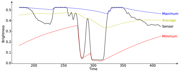
Figure 6: Example of rolling minimum, maximum, and average

3.3.2 RNNs Recognizing Phases of Gestures

An RNN can also be used to recognize parts of gestures instead of entire gestures. Phases can be recognized with a finite state machine (FSM) implemented as recurrent neural layer. The states need to be defined manually and implemented as neurons. Transitions can be learned as weights and biases from training data. Each gesture can be split into five phases assuming a 3x3 light sensor. The gestures have similar phases, explained in the following for the gesture of moving the hand from left to right (see Fig. 7). Its first phase ends, when the hand reaches the left column of the sensor matrix. The second ends when the middle column is reached. The third optional phase ends, when the hand reaches the right column and then covers all columns. It is optional, as the gesture can be made with a single finger that already no longer covers the first column when it reaches the third. The fourth phase ends, when the hand covers the right column but no longer the first one. The fifth and final phase ends when the hand has passed the right column. Then the complete gesture has ended. The phases of the other gestures are the same but rotated by $\pm$90 or 180 degrees.

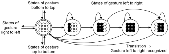
Figure 7: Finite state machine for recognizing the gesture of moving the hand from left to right

The used FSM has 17 states: an initial state and four states for each of the four gestures. The initial state and the four states of a gesture correspond to the five phases. The initial state corresponds to the first phase of all gestures. The transition that leaves this phase determines the gesture to be recognized. When the hand leaves the right column in the fifth phase, the transition to the initial state means, that the gesture was recognized. Transitions from the other states back to the initial state are possible in cases where a movement was an invalid gesture.

In a preliminary experiment, the FSM was implemented for a hand gesture sensor module without machine learning. Unfortunately, it achieved a low reliability only. A threshold value was used to determine whether the hand is in front of one sensor. The hand is assumed to be in front of a row or column, if it is in front of at least two of its sensors. Covered rows and columns were used to decide about triggering transitions of the FSM. Even under good illumination conditions with direct back-lighting the recognition was unreliable. Often, the end of the first phase was not recognized or attributed to a wrong gesture. It can be assumed that a trained RNN is more reliable, as pre-processing of sensor data and transitions can be better trained from recorded gestures.

For machine learning, the FSM can be implemented as recurrent layer. Each state is realized as a neuron that is activated when the FSM is in that state. The feedback of the recurrent layer is necessary to maintain the state of the FSM. The inputs of the layer allow triggering or blocking transitions. Activation function Softmax seems appropriate, as the activation of a neuron can then be regarded as the probability that the FSM is in the corresponding state. This allows the FSM to be in different states at the same time with a certain probability. However, experiments showed that there is almost always only one state with a probability close to one.

For detecting phases of gestures, the recurrent layer implementing the FSM needs to be the output layer, see Fig. 8. A gesture is recognized when the biggest activation of the output layer indicates the last state of a gesture in one step and the initial state in the next. Software can be written manually to detect this. One or two hidden layers are reasonable to pre-process sensor data. The features are the same as for the RNN in Sec. 3.3.1.

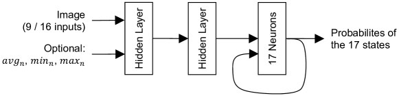
Figure 8: RNN for recognizing phases of gestures

3.3.3 FFNNs

The approach for gesture recognition using FFNNs in this study uses two algorithms. The first detects the start and the end of sequences of images that potentially represent a gesture. The sequences with a varying number of images are stored in a buffer. The second algorithm scales the buffer to a fixed number of images to be used as features to simplify classification. Sequences of images that potentially contain a gesture are called candidates. Extracting candidates reduces processing time, as the FFNN is only executed for candidates. Another advantage is that the processing times of the FFNN may be longer than the image sampling interval. In this case, one or several images may get lost. However, this is acceptable, as there is always a gap of several images between gestures.

The algorithm for extracting candidates is based on the observation, that the average brightness of images decreases when the hand is in front of the camera. The algorithm searches for sequences of images where the brightness deviates from a rolling average by at least 10%. If at least nine images belong to such a sequence, five images are added before and after it. Each such sequence is a candidate. The rolling average is calculated from the average brightness of images deviating from the rolling average less than 10%. Thus, candidates do not change it. To avoid short outliers, images are only considered if their average brightness differs by less than 1% from the previous. Experiments showed that the algorithm reliably isolates candidates even under different lighting conditions. They also revealed that adding five images before and after the initial sequence was appropriate to capture an entire gesture.

As candidates contain different numbers of images, these are scaled to a fixed number of images. The alternative is filling the buffer with null values to get a fixed number of features for the FFNN. However, in this case the FFNN is required to find information determining the gesture at different locations in the buffer, increasing the difficulty of the classification. A simple approach for scaling to a fixed number of images is deleting excess images or duplicating missing ones evenly throughout the sequence of a candidate. However, this leads to unreal sequences, as if the hand is not moving with constant speed.

The algorithm used for this study, scales candidates by linearly interpolating 20 images from adjacent recorded images. This leads to realistic sequences of images as the brightness of the light sensors changes continuously with the movement of the hand. 20 points in time are selected for the desired images at equal intervals from the first to the last recorded image of a candidate. This is illustrated in Fig. 9 for a candidate starting at time 2 and ending at time 14. The time is normalized to the recording times of the images leading to integer times for recorded images. However, the points in time of the 20 interpolated images are not necessarily integral. The value $S_{t,i}$ of the $i^{th}$ sensor at point in time t is linearly interpolated from the values $S_{\lfloor t\rfloor,i}$ and $S_{\lfloor t\rfloor+1,i}$ of the adjacent recorded images with equation (6). This is illustrated in Fig. 9 for $t=3.26$.

$$S_{t,i}=S_{\lfloor t\rfloor,i}(\lfloor t\rfloor+1-t)+S_{\lfloor t\rfloor+1,i}(t-\lfloor t\rfloor)$$ (6)

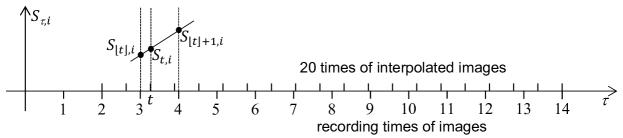
Figure 9: Linear interpolation for scaling candidates of gestures

The FFNN classifying the scaled buffer has 180 features and five output neurons. The features are the 9 light values of the 20 images normalized to $[0,1[$. The maximum activation of the five output neurons indicates the four gestures resp. no gesture.

3.4 Training Data

For the three approaches, the training data needs to be annotated in a different way. Recorded sequences have to be annotated with the expected output of the ANNs. This has to be done manually and should be supported by software simplifying the task. The expected output is the gestures for RNNs and FFNNs. However, for the RNN recognizing phases of gestures, it is the expected phases. To avoid false classifications of movements that are not intended as gestures, many different variants of such false movements have to be recorded and annotated accordingly.

So-called synthetic training data should be added to facilitate the laborious task of recording and annotating training data. In general, synthetic training data is computed from recorded and annotated training data by transforming it in a way, so that the annotation remains the same or can be automatically updated. Frequently noise is added to sensor values. In training data with respect to gestures, brightness, contrast, or gamma value can be changed, images can be mirrored on the X or Y axis or turned by $\pm 90^{\circ}$ or $180^{\circ}$. These operations can also be combined. After these changes, the annotations can be automatically updated. Experiments show that extending the training data with synthetic training data improves the accuracy of classifications considerably.

Recorded sequences of images for training RNNs have to be annotated with the gestures to be recognized. Annotations are added to the last image of a gesture. This is the point in time, when the gesture should be recognized. However, in practice, an RNN may recognize the gesture a few images earlier or later. For RNNs recognizing phases, training data has to be annotated with the phases. This requires a person to observe the recorded videos and add the expected phase to each image. For these decisions, the person has leeway, as the transitions are not always clearly visible. The RNN thus learns the intuition of this person. The laborious work required for annotation is a major drawback of this approach.

For FFNNs, the algorithm for extracting candidates of gestures massively simplifies annotating training data. Annotations only need to be added to each candidate found by the algorithm. If the same sequence of gestures is repeated over and over again, annotations can still be added automatically. For example, in this study, the gestures from left to right and from right to left were repeatedly recorded alternately one after the other, as this movement is easy to perform.

4 Validation

The three approaches for recognizing gestures on sensor modules with ANNs have been implemented and validated: Two RNNs recognizing gestures or phases of gestures respectively, and an FFNN recognizing gestures. The hardware for a sensor module has been developed, used to record data to train and test the ANNs, and to execute them. The solution with an FFNN leads to the most accurate gesture recognition.

4.1 Experimental Hand Gesture Sensor Module Hardware

The hand gesture sensor module implements a compound eye camera with a black tube in front of each light sensor to provide directivity as illustrated in Fig. 10. The use of a lens or a camera chip was rejected for price and simplicity reasons. The tubes are manufactured as part of the device’s housing.

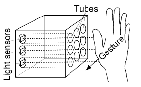
Figure 10: Gesture recognition with a compound eye camera

The compound eye camera sensor module is a printed circuit board (PCB) with few components only, that is, a microcontroller, up to 16 light sensors (phototransistors), the same number of resistors, and three diodes. A simplified schematic circuit diagram is given in Fig. 11. Its microcontroller ATMega4809 [12] is slightly more powerful than the ATmega328P discussed in Sec. 2.2.4. It has a clock speed of up to 20 MHz, 6 kB of RAM, and 48 kB of flash memory. It has neither a floating-point unit nor a memory cache. Its 16 AD channels with 10-bit resolution allow connecting each light sensor to its own channel. This allows a resolution of up to 4x4 pixels, however, 3x3 pixels are used in this work. The sensor module has 3 connectors providing a Unified Program and Debug Interface (UPDI), a UART and 8 GPIO lines that can also be used as I²C or SPI. The double layer PCB has a size of 33 x 38 millimeters. With its 3D printed housing shown in Fig. 12 its size is 4 x 4 x 2 centimeters with tubes of length of 1 cm, diameter of 5 mm, and distance of 7 mm.

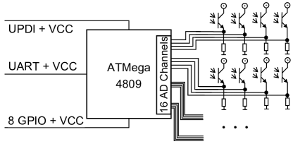
Figure 11: Simplified schematic circuit diagram of compound eye camera sensor module with 4x4 pixels

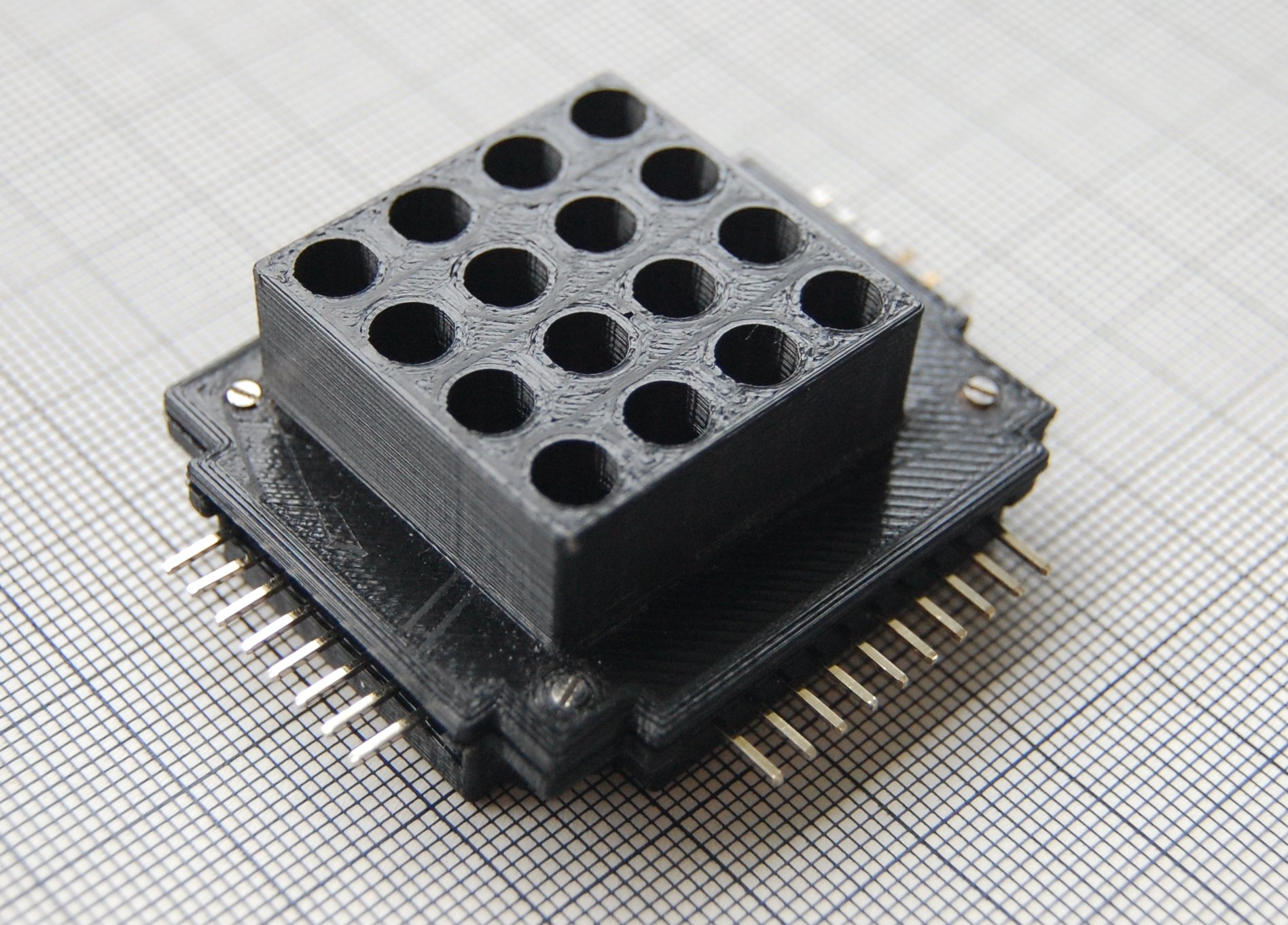
Figure 12: Compound eye camera sensor module with 4x4 pixels

A preliminary version of the prototype was used for the experiments described in subsequent sections. It was built from an Arduino board and 3x3 light sensors. The Arduino Uno board [1] contains the microcontroller ATmega328P introduced in Sec. 2.2.4. To be able to connect 9 light sensors to its 6 AD channels, light sensors are organized in rows that are activated with IO pins.

4.2 Procedure for Validation

For all approaches, many ANNs were trained and tested to find the best accuracy still allowing an efficient execution to enable a frame rate of 40 frames per second. The following entities were varied during validation: number of hidden layers, number of neurons per hidden layer, activation function, and the number of repetitions of the training (epochs). For RNNs, we analyzed whether including the optional features $avg_{n},min_{n},max_{n}$ leads to better accuracy. In the following, we refer to these three features simply as the optional features. Training and validation were performed with Keras and TensorFlow using the optimizer Adam.

The same training data was used for RNNs recognizing gestures and phases with different annotations. The data was based on 15 recordings of each gesture from different distances, performed with a finger, the entire hand, or an arm. In addition, movements that do not correspond to one of the gestures were recorded and classified as no gesture. Synthetic training data was produced from the recorded data by mirroring and rotating the images, and by changing brightness and gamma value. This led to 540 instances of each gesture.

Training data for the FFNNs was automatically annotated using fixed repetitions of two gestures and the algorithm for extracting candidates. These repetitions were the alternation of the gestures from left to right and from right to left as well as from top to bottom and from bottom to top. Thus, for each extracted candidate, the gesture was known and could be annotated automatically. 350 gestures and non-gestures were recorded with direct back-lighting and against backgrounds of varying brightness with distances between 5 and 30 cm between hand and camera. Synthetic training data increased the number of gestures by a factor of four.

For all three approaches, the same metric to assess the accuracy is used. It is measured by executing the ANNs for the same test set of gestures recorded independently of the training set. Accuracy is expressed as the percentage of correctly recognized gestures. A gesture is considered correctly recognized, if it is recognized approximately at the expected point in time (at most 10 images before or after). Correctness of the entire gesture is also the relevant measure for RNNs recognizing phases. The test set contained 24 recordings of each gesture, recorded from four distances between hand and sensor module (3 cm, 15 cm, 20 cm, and 30 cm) at two brightness levels of the illumination. Gestures are more blurred for longer distances and stand out less from the background noise at lower brightness.

4.3 Results

The experiments show, that an FFNN leads to the highest accuracy of 83% requiring 1480 multiplications. RNNs recognizing phases allow an accuracy up to 71% with about half of the number of multiplications. The accuracy decreased by 10 (resp. 14) percentage points for RNNs directly recognizing gestures using a huge (resp. moderately sized) RNN. Best accuracies for RNNs always required the optional features. Only the FFNN can be used for practical applications with good illumination.

4.3.1 RNNs Recognizing Gestures

The analyzed RNNs had up to three recurrent hidden layers, $2^{2}$ to $2^{7}$ neurons and used one of the activation functions Tanh, Sigmoid, Softsign, or Hard Sigmoid. Function Relu was discarded as preliminary experiments showed that it leads to numeric overflows due to an ever-increasing feedback of recurrent layers. The best accuracy of 61% was observed for an RNN with two hidden layers, 128 neurons each, and the optional features. However, it had a large computational effort for execution and required a considerable amount of memory, see Tab. 4 for details. An RNN requiring only 7% of the resources allowed an accuracy of 57%. The demand of resources was again 50% lower for an RNN with a single hidden layer yielding an accuracy of 56%. Another RNN with a single hidden layer even enabled an accuracy of 59%, that is close to the best RNN. However, despite the minimal number of layers, it also required a lot of resources.

Table 4: Accuracies achieved for RNN architectures recognizing gestures

Accuracy	Optional Features	No. of Hidden   Layers (H.L.)	No. of Neu- rons per H.L.	Activation Func- tion (A.F.) of H.L.	Calls of      A.F.	Multipli-   cations	No. of Parameters
61%	Yes	2	128	Hard Sigmoid	256	51328	51589
57%	Yes	2	32	Softsign	64	3616	3685
56%	Yes	1	32	Tanh	32	1568	1605
59%	Yes	1	128	Sigmoid	128	18650	18783
52%	No	1	32	Tanh	32	1472	1509
52%	No	2	16	Softsign	32	1040	1077
58%	Yes	3	128	Softsign	384	84096	84485

Including the optional features usually led to a higher accuracy. The average accuracy in this case was 8 (resp. 7, 15) percentage points higher than without for RNNs with one (resp. two, three) hidden layer, assuming at least 16 neurons per hidden layer. Increasing the number of hidden layers from two to three did not increase the accuracy. With three, the best accuracy was 58%. This is three percentage points less than the best observed accuracy for two hidden layers, although requiring more resources. Increasing the number of hidden layers from two to three reduced the accuracy from 48% to 44% on average assuming at least 16 neurons per layer. The average accuracy with one hidden layer was also 44%.

The best observed accuracy of 61% is by far not sufficient for practical applications using gesture recognition. We regard it as unlikely that changing the numbers of neurons in hidden layers, also varying among the layers, nor more training runs will improve the results significantly. It is reasonable to assume that the well-known vanishing gradient problem is the reason why the training does not lead to RNNs with better accuracy. Hochreiter described this problem already in 1998. RNNs trained with back-propagation cannot learn problems that require combining inputs too many processing steps apart (long time lag problems) [8]. The reason is, that corrections on weights and biases continuously get smaller as they are propagated from time step to time step during training. A common solution is Long Short-Term Memory (LSTM) networks [9], keeping these corrections constant. However, these were rejected for this study due to the higher computational effort.

As a result, training RNNs for gesture recognition with the approach described above, is not considered appropriate. Gestures cannot be recognized reliably, as parts of the gestures are contained in images too far apart. Nevertheless, this does not mean that the approach is not applicable to other classification problems, in which classes depend on sensor values measured in short succession.

4.3.2 RNNs Recognizing Phases of Gestures

With RNNs recognizing phases of gestures, a better accuracy of 71% was observed with two hidden non-recurrent layers each with nine neurons, activation function Relu and the optional features. It requires only 631 multiplications and 18 Relu function calls during execution, and has 666 parameters. This is significantly less than for the best RNNs directly recognizing gestures, making the RNN more suitable for small microcontrollers. As in Sec. 4.3.1, leaving out the optional features reduces accuracy to 59%. Using recurrent hidden layers instead of the non-recurrent layers does not improve accuracy.

To investigate the required number of neurons for the hidden layers, all 9 combinations of 4, 9, and 16 neurons were tested for the two layers. Using 16 instead of 9 neurons did not improve the accuracy. With only 4 neurons in one of the layers the accuracy fell to 60%. Using a single hidden layer with 9 neurons only further decreased the accuracy. The activation function Relu was chosen for the hidden layers, as it led to the best accuracy and can be executed very fast on a microcontroller. Sigmoid and Softsign reduced the accuracy from 71% to 65% and to 64% for Hard Sigmoid.

The above numbers assume the approximated version of Softmax (see Sec. 2.2.4) as activation function for the output layer implementing the finite states machine. Using the normal version of Softmax only led to an accuracy of 69%. Replacing Softmax with the fast-executable Max could have worked for this recurrent layer, as the use of Softmax leads to activations close to 0 or 1 in practice, which are the results of Max. But, when using Max, the accuracy decreased to 61%.

With an accuracy of 71%, the approach of recognizing phases of gestures led to a better result than training RNNs to recognize gestures directly. We assume that the vanishing gradient problem has less impact on recognizing phases than gestures, because the images required for that are closer together. Recognition of phases also led to a smaller RNN.

However, 71% accuracy is still not sufficient for practical applications. The RNN was implemented for the hand gesture sensor module from Sec. 4.1. Experiments showed that the sensor module recognizes most but not all gestures under good illumination with direct back-lighting. With unfavorable illumination, an unacceptable proportion of gestures is not recognized correctly.

4.3.3 FFNNs

For the FFNN, a single hidden layer with 8 neurons was chosen, achieving an accuracy of 83%. Relu was selected as activation function for the hidden layer and Max for the output layer. Despite the low number of neurons, the FFNN still requires 1480 multiplications because of its 180 features. The number of hidden layers and its neurons was chosen in a preliminary study. It compared FFNNs with one or two hidden layers and 5 to 20 neurons. For a simple test set, this led to the accuracy values shown in Tab. 5. A single layer with 8 neurons was chosen to keep the computational effort low.

Table 5: Accuracies achieved of FFNN architectures

Accuracy	No. of Hidden   Layers (H.L.)	No. of Neurons        in 1st H.L.	No. of Neurons        in 2nd H.L.	Calls of Relu	Multipli-   cations	No. of Parameters
84%	1	5	-	5	925	935
98%	1	8	-	8	1480	1493
99%	1	10	-	10	1850	1865
100%	1	15	-	15	2775	2795
100%	1	20	-	20	3700	3725
100%	2	10	10	20	1950	1975
100%	2	20	10	30	3850	3885

The FFNN was implemented for the sensor module with 3x3 pixels from Sec. 4.1 including the extraction and scaling of candidates. Experiments with that module revealed that candidates can be reliably extracted up to distances of 90 cm between hand and camera, assuming good illumination with direct back-lighting. The accuracy decreases with increasing distance. It was 100% up to 20 cm, 83% at 40 cm, 58% at 70 cm, and 8% at 90 cm. In the case of misclassifications, incorrect gestures were recognized more often than no gesture. Less bright, flatter light reduces the distance at which gestures can be reliably recognized. An uneven background does not change the accuracy, unless it has a very high contrast (e.g. a checkerboard pattern).

Measurements showed an execution time of 47 ms to process a candidate, 11 ms for scaling and 36 ms to process the FFNN. This is approximately twice the image sampling rate of 25 ms, since 40 images are recorded per second. At least one image gets lost. However, this does not matter in practice due to the gap of several images between candidates.

The 2 kB RAM and 32 kB flash memory of the ATMega328P microcontroller proved to be sufficient. For the FFNN, a naïve implementation with 32-bit floating-point numbers was used. The 1493 parameters require 5972 bytes of the flash memory. 1440 bytes of the RAM were used for the buffer storing light values of up to 80 images (2 seconds) of a candidate of a gesture. In the buffer, light values are stored as 16-bit integers as provided by the AD converter and normalized to float later to save memory. After a candidate is found, the memory of the buffer is reused for storing the scaled candidate and intermediate values of the FFNN.

The approach of using an FFNN for gesture recognition with buffering and scaling of candidates has several advantages. It leads to the best accuracy of 83% in this study. Its execution is efficient, also allowing to lose a few images between candidates. It simplifies annotating training data. However, this came at the effort of developing two algorithms to extract and scale candidates. Buffering also requires a large amount of RAM.

4.4 Compression

The previous sections showed that ANNs can be implemented for small microcontrollers in a straightforward way without much optimization, provided that the ANNs are sufficiently small and there is sufficient time for their execution. However, further optimizations are necessary if higher accuracies require bigger ANNs or if an application requires shorter execution times. Rockschies analyzed this in the context of this study by applying deep compression (see Sec. 2.2.5) to an FFNN for hand gesture recognition [24]. Pruning and quantization reduced the memory size for the parameters by a factor 6, with no significant influence on the execution time. Encoding the parameters in a sparse matrix format reduced the memory size by the same factor but also halved the execution time. Huffman encoding reduced the memory size by another 34% but increased the execution time by a factor of five compared to the original FFNN.

The FFNN used for the experiments had the same 180 features (20 images with 9 pixels each) as discussed in Sec. 3.3.3. It had two hidden layers with 7 and 14 neurons. Its output layer has 13 neurons as the FFNN classifies into 12 gestures. Without compression it requires 1540 multiplications for execution, leading to a measured execution time of 24.5 ms. The 1574 parameters require 6.296 kB of flash memory and 11 kB for the entire program. Pruning and quantization slightly decreased the accuracy from 96.9% to 94.6%. Pruning removed 68% of the edges. Weights were quantized to 15 clusters encoded in 4 bits. With the encoding described in Sec. 2.2.5, the model required 1.098 kB of flash memory to encode the parameters and 6.1 kB for the entire program. The execution time slightly increased to 27.8 ms.

The weights of each layer were also encoded in a sparse matrix format that can be classified as an address map scheme [21]. This allowed encoding the parameters in 1.053 kB of flash memory and the entire program in 6.4 kB. It also halved the execution time of the FFNN to 12.6 ms, as multiplications only need to be applied to the non-null weights. The format encodes the weight matrix of a layer in two arrays, the first containing the non-null values of the matrix and the second describing the position of each non-null value in the matrix. Conceptually, the matrix is first linearized row by row into a one-dimensional array as illustrated for an example in Fig. 13. The position of each non-null value in the second matrix is encoded as the difference of its index to the index of the previous value.

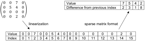
Figure 13: Example of the sparse matrix format used for compression

Deep compression of the model for gesture recognition does not allow the compression rates achieved for the large models discussed in Sec. 2.2.5. The model for gesture recognition only allowed pruning of 68% of the edges, while the larger AlexNet allowed 89% and VGG-16. 92.5%. Hence the model could only be compressed to 11.5% instead of 2.88% for AlexNet and 2.05% for VGG 16 (including Huffman encoding). The authors assume that in general, smaller models can be compressed less than larger ones as these models have typically less redundancy.

5 Developing Sensor Modules using ANNs

ANNs can be executed on small microcontrollers with straightforward implementations based on 32-bit floating-point numbers. However, this assumes that the architecture of the ANN is not too large to fit into the memory and that response times required by the application are sufficiently long. If sequences of sensor values are to be classified, FFNNs with buffers are the best choice. An RNN should only be used if the sensor values determining the class are close in time. A rigorous workflow should be applied. The first stage is the acquisition of training data annotated with the desired classes. The architecture of the ANNs should be determined, trained, and then validated. If necessary, ANNs can be compressed and again validated. Finally, the ANN has to be implemented for a particular microcontroller.

However, some experimentation will be necessary to find a suitable architecture providing adequate classifications with a low computation effort. There are no straightforward rules for deciding on architectures. Using more layers does not necessarily lead to better classifications nor does it generally imply a higher computational effort. The choice of an activation function is one means to reduce execution time; Relu and Max are good candidates. Creating training data is often time-consuming. Therefore, a sensor module hardware and the corresponding recording software must be developed. The sensor module must be deployed in a realistic environment for recording. Adding the expected classes to recordings is another major effort, especially if it needs to be performed by hand. If it is impossible to produce large amounts of training data, synthetic training data is a good means to get more data to improve training.

Several options exist in case a straightforward implementation of an ANN requires too many resources for a particular microcontroller. An obvious option is a more powerful microcontroller, especially with FPU or hardware-operations for efficiently executing matrix operations (e.g. Multiply-And-Accumulate). Otherwise, models can be compressed (see Sec. 2.2.5). Libraries (e.g. [14]) or specialized compilers (e.g. [6]) can be applied to optimize the execution on the microcontroller. One can also consider using other ML methods, such as decision trees [26], Bayesian networks [15], k-nearest neighbors [20, 26, 28], or support vector machines [26].

6 Conclusion

The paper showed that it is possible to execute an ANN on a low performance microcontroller with few kilobytes of RAM assuming that the classification problem is sufficiently simple. Sensor modules can be implemented using ANNs to classify time sequences of sensor values. This was shown for a sensor module recognizing hand gestures using nine light sensors as a simple camera, with the best ANN having only 13 neurons and 1493 parameters, requiring an execution time of 36 ms.

Continuous time sequences of sensor values can be classified with RNNs or FFNNs. RNNs naturally map to processing sequences. FFNNs were used by buffering a part of the sequence of sensor values in memory that is considered as a candidate of a gesture. This buffer forms the input to the FFNN for classification.

The preferred approach from this study is using an FFNN, because this can be implemented without special effort and leads to the most reliable classification correctly identifying 83% of the gestures. It also required less processing power, as the FFNN is executed only after a promising sequence is detected by a manually written algorithm. Reliable classification with an RNN (correctly identifying 71% of the gestures) was only possible after solving a part of the classification problem manually – that is – by splitting gestures into five phases. Therefore, the meaning of the activations of some of the neurons had to be defined and training data had to be laboriously annotated.

An 8-bit microcontroller without a floating-point unit was sufficient to execute RNNs and FFNNs with only 2 kB of RAM, 32 kB of flash memory, and a clock cycle of 16 MHz. This enabled a frame rate of 40 Hz, which was sufficient for the application without using optimization techniques such as pruning and quantization. However, the reliability of the classification significantly deteriorated with degrading lighting conditions.

References

- [1] Arduino. Arduino uno rev3. arduino s.r.l., 2020. URL: https://store.arduino.cc/arduino-uno-rev3.
- [2] Atmel Corporation. Atmega328p – 8-bit avr microcontroller with 32k bytes in-system programmable flash – datasheet, 2015. URL: http://ww1.microchip.com/downloads/en/DeviceDoc/Atmel-7810-Automotive-Microcontrollers-ATmega328P_Datasheet.pdf.
- [3] F. Ertam and G. Aydın. Data classification with deep learning using tensorflow. In 2017 International Conference on Computer Science and Engineering (UBMK), pages 755–758, 2017. doi:https://doi.org/10.1109/UBMK.2017.8093521.
- [4] Rui Fu, Zuo Zhang, and Li Li. Using lstm and gru neural network methods for traffic flow prediction. In 2016 31st Youth Academic Annual Conference of Chinese Association of Automation (YAC), pages 324–328, 2016. doi:https://doi.org/10.1109/YAC.2016.7804912.
- [5] Ian Goodfellow, Yoshua Bengio, and Aaron Courville. Deep Learning. MIT Press, 2016. http://www.deeplearningbook.org.
- [6] Sridhar Gopinath, Nikhil Ghanathe, Vivek Seshadri, and Rahul Sharma. Compiling kb-sized machine learning models to tiny iot devices. In Proceedings of the 40th ACM SIGPLAN Conference on Programming Language Design and Implementation, PLDI 2019, page 79–95, New York, NY, USA, 2019. Association for Computing Machinery. doi:10.1145/3314221.3314597.
- [7] Song Han, Huizi Mao, and William J. Dally. Deep compression: Compressing deep neural network with pruning, trained quantization and huffman coding. ArXiv, abs/1510.00149, 2015. URL: http://arxiv.org/abs/1510.00149.
- [8] Sepp Hochreiter. The vanishing gradient problem during learning recurrent neural nets and problem solutions. Int. J. Uncertain. Fuzziness Knowl.-Based Syst., 6(2):107–116, April 1998. doi:10.1142/S0218488598000094.
- [9] Sepp Hochreiter and Jürgen Schmidhuber. Long short-term memory. Neural Comput., 9(8):1735–1780, November 1997. doi:10.1162/neco.1997.9.8.1735.
- [10] Martin Holmberg, Fredrik Gustafsson, E. Gunnar Hörnsten, Fredrik Winquist, Lennart E. Nilsson, Lennart Ljung, and Ingemar Lundström. Bacteria classification based on feature extraction from sensor data. Biotechnology Techniques, 12, 1998. doi:https://doi.org/10.1023/A:1008862617082.
- [11] David A. Huffman. A method for the construction of minimum-redundancy codes. Resonance, pages 91–99, 2006. doi:https://doi.org/10.1007/BF02837279.
- [12] Microchip Technology Incorporate. Atmega4808/4809 data sheet, 2020. URL: http://ww1.microchip.com/downloads/en/DeviceDoc/ATmega4808-4809-Data-Sheet-DS40002173A.pdf.
- [13] Philipp Jantscher. Ai in sensors for iot. silicon semiconductor, 2019. URL: https://siliconsemiconductor.net/article/106227/AI_In_Sensors_For_IoT.
- [14] Liangzhen Lai, Naveen Suda, and Vikas Chandra. Cmsis-nn: Efficient neural network kernels for arm cortex-m cpus. ArXiv, abs/1801.06601, 2018. URL: https://arxiv.org/abs/1801.06601.
- [15] Charles Leech, Yordan P. Raykov, Emre Ozer Ozer, and Geoff V. Merrett. Real-time room occupancy estimation with bayesian machine learning using a single pir sensor and microcontroller. In 2017 IEEE Sensors Applications Symposium (SAS), pages 1–6, 2017. doi:https://doi.org/10.1109/SAS.2017.7894091.
- [16] J. MacQueen. Some methods for classification and analysis of multivariate observations. In Proceedings Fifth Berkeley Symposium on Mathematical Statistics and Probability, Vol. 1: Statistics, pages 281–297, Berkeley, Calif., 1967. University of California Press. URL: https://projecteuclid.org/euclid.bsmsp/1200512992.
- [17] Vinod Nair and Geoffrey E. Hinton. Rectified linear units improve restricted boltzmann machines. In Proceedings of the 27th International Conference on International Conference on Machine Learning, page 807–814, Madison, 2010. URL: https://icml.cc/Conferences/2010/papers/432.pdf.
- [18] Michael A. Nielsen. Neural networks and deep learning, determination press, 2017. URL: http://neuralnetworksanddeeplearning.com/.
- [19] Juan Pardo, Francisco Zamora-Martínez, and Paloma Botella-Rocamora. Online learning algorithm for time series forecasting suitable for low cost wireless sensor networks nodes. Sensors, 15 (4), 2015. doi:https://dx.doi.org/10.3390/s150409277.
- [20] Shishir G. Patil, Don Kurian Dennis, Chirag Pabbaraju, Nadeem Shaheer, Harsha Vardhan Simhadri, Vivek Seshadri, Manik Varma, and Prateek Jain. Gesturepod: Enabling on-device gesture-based interaction for white cane users. In Proceedings of the 32nd Annual ACM Symposium on User Interface Software and Technology, UIST ’19, page 403–415, New York, 2019. Association for Computing Machinery. doi:10.1145/3332165.3347881.
- [21] Udo W. Pooch and Al Nieder. A survey of indexing techniques for sparse matrices. ACM Comput. Surv., 5(2):109–133, June 1973. doi:10.1145/356616.356618.
- [22] Bernhard Preim and Raimund Dachselt. Interaktive Systeme Band 2: User Interface Engineering, 3D-Interaktion, Natural User Interfaces. 2nd edition. Springer Vieweg, 2015. URL: https://www.springer.com/de/book/9783642452468.
- [23] Sony Corporation Press release. Sony to release world’s first intelligent vision sensors with ai processing functionality, 2020. URL: https://www.sony.net/SonyInfo/News/Press/202005/20-037E/.
- [24] Marius Rockschies. Minimal Execution Time of Artificial Neural Networks on Resource-Restricted Devices. Master’s thesis, Hamburg University of Technology, Germany, 2003.
- [25] Wolfgang Roth, Günther Schindler, Matthias Zöhrer, Lukas Pfeifenberger, Robert Peharz, Sebastian Tschiatschek, Holger Fröning, Franz Pernkopf, and Zoubin Ghahramani. Resource-efficient neural networks for embedded systems. ArXiv, abs/2001.03048, 2020. URL: https://arxiv.org/abs/2001.03048.
- [26] Fouad Sakr, Francesco Bellotti, Riccardo Berta, and Alessandro De Gloria. Machine learning on mainstream microcontrollers. Sensors, 20 (9), 2019. doi:https://doi.org/10.3390/s20092638.
- [27] Khaled Saleh, Mohammed Hossny, and Saeid Nahavandi. Driving behavior classification based on sensor data fusion using lstm recurrent neural networks. In 2017 IEEE International Conference on Intelligent Transportation Systems, pages 1–6, 2017. doi:https://doi.org/10.1109/ITSC.2017.8317835.
- [28] Vignesh M. Suresh, Rishi Sidhu, Prateek Karkare, Aakash Patil, Zhang Lei, and Arindam Basu. Powering the iot through embedded machine learning and lora. In 2018 IEEE 4th World Forum on Internet of Things (WF-IoT), pages 349–354, 2018. doi:https://doi.org/10.1109/WF-IoT.2018.8355177.
- [29] Bosch Security Systems. Radion tritech. data sheet, 2018. URL: http://resource.boschsecurity.com/documents/RADION_TriTech_Data_sheet_enUS_11161300619.pdf.
- [30] Jindong Wang, Yiqiang Chen, Shuji Hao, Xiaohui Peng, and Lisha Hu. Deep learning for sensor-based activity recognition: A survey. Pattern Recognition Letters, 119:3 – 11, 2019. URL: http://www.sciencedirect.com/science/article/pii/S016786551830045X, doi:https://doi.org/10.1016/j.patrec.2018.02.010.
- [31] Xuyu Wang, Zhitao Yu, and Shiwen Mao. Deepml: Deep lstm for indoor localization with smartphone magnetic and light sensors. In 2018 IEEE International Conference on Communications (ICC), pages 1–6, 2018. doi:https://doi.org/10.1109/ICC.2018.8422562.
- [32] Rui Zhao, Ruqiang Yan, Jinjiang Wang, and Kezhi Mao. Learning to monitor machine health with convolutional bi-directional lstm networks. Sensors, 17 (2), 2017. doi:https://doi.org/10.3390/s17020273.
- [33] Yu Zhao, Rennong Yang, Guillaume Chevalier, Ximeng Xu, , and Zhenxing Zhang. Deep residual bidir-lstm for human activity recognition using wearable sensors. Advancements in Mathematical Methods for Pattern Recognition & Applications, 2018. doi:https://doi.org/10.1155/2018/7316954.