Evolution of a passive particle in a one-dimensional diffusive environment

Abstract.

We study the behavior of a tracer particle driven by a one-dimensional fluctuating potential, defined initially as a Brownian motion, and evolving in time according to the heat equation. We obtain two main results. First, in the short time limit, we show that the fluctuations of the particle become Gaussian and sub-diffusive, with dynamical exponent $3/4$. Second, in the long time limit, we show that the particle is trapped by the local minima of the potential and evolves diffusively i.e. with exponent $1/2$.

1. Introduction

Random walks in dynamical random environments have attracted a lot of attention recently. When the time correlations of the environment decay fast, several homogenization results have been obtained, see [21][5] as well as references therein. These results establish the existence of an asymptotic velocity for the walker (law of large numbers) and normal fluctuations around the average displacement (invariance principle). In the opposite extreme regime, when the environment becomes static, a detailed understanding of the behavior of the walker is available in dimension $d=1$, see e.g. [25] for a review.

Diffusive environments in dimension $d=1$ constitute an intermediate case where memory effects are expected to become relevant, since correlations decay only with time as $t^{-1/2}$. Homogenization results are known when the walker drifts away ballistically, and escapes from the correlations of the environment [12][6][16][22]. Recently, among other results, a law of large number with zero limiting speed was derived in [13], for the position of a walker evolving on top of the symmetric simple exclusion process (SSEP). However, the question of the size of the fluctuations in such a case remains largely elusive, and several conflicting conjectures appear in the literature [7][10][20][4][15]. In a particular scaling limit, Gaussian anomalous fluctuations were shown to hold for a walker on the SSEP [17], see also below.

The aim of this paper is to advance our understanding on the fluctuations of a walker in an unbiased, one-dimensional, diffusive random environment, and to make clear that different behaviors may be observed depending on the time scales that we look at. For this, we introduce a new model where the evolution of the walker can be described in a fair bit of detail. To motivate properly the introduction of this new model, let us start with a question that, we believe, is of more fundamental interest.

Motivation — Let us consider a random potential $V=(V(t,x))_{t\geq 0,x\in\mathbb{R}}$ fluctuating with time according to the stochastic heat equation:

(1.1) $$\begin{cases}V(0,x)\;=\;B(x),\\ \partial_{t}V(t,x)\;=\;\partial_{xx}V(t,x)+\sqrt{2}\xi(t,x)\end{cases}$$

where $B$ is a Brownian motion on $\mathbb{R}$, and where $\xi(t,x)$ is a space-time white noise. We refer to [11] for a gentle introduction to the stochastic heat equation. The process $V$ is stationary, i.e. $V(t,\cdot)$ is distributed as $B(\cdot)$ at all times $t\geq 0$, and evolves diffusively in time, i.e. the landscape described by $V(t,\cdot)$ in a box of size $L$ is refreshed after a time of order $L^{2}$. The potential $V$ solving (1.1) can be obtained as the scaling limit of the height function of diffusive particle processes on the lattice, such as the SSEP, see e.g. Chapter 11 in [18].

We would like to consider a process $X=(X_{t})_{t\geq 0}$ describing a particle driven by this potential in the overdamped regime:

(1.2) $$\begin{cases}X_{0}\;=\;0,\\ \partial_{t}X_{t}\;=\;-\partial_{x}V(t,X_{t})\;=:\;u(t,X_{t})\end{cases}$$

Since $V(t,\cdot)$ is rough, it is however not clear that the evolution equation (1.2) makes sense, and three natural questions arise:

1. Can the process $X$ be properly defined?

2. If yes, how does it behave on short time scales?

3. And how does it behave in the long time limit?

We notice that, in the presence of an external random force, the analogous process in a static environment is well defined: There exists a process $X^{\text{st}}$ solving

$$X^{\text{st}}_{0}\;=\;0,\qquad\text{\rm d}X^{\text{st}}_{t}\;=\;-\partial_{x}V(0,X^{\text{st}}_{t})\text{\rm d}t+\text{\rm d}\widetilde{B}_{t}$$

almost surely for all $t\geq 0$, where $(\widetilde{B}_{t})_{t\geq 0}$ is a Brownian motion independent of $B$ [8][14]. Moreover, the long time behavior of $X^{\text{st}}$ is analogous to that of Sinai’s random walk [23].

As far as we know, the above questions were first addressed in [7] by means of a heuristic fixed point argument. First, the authors conclude that if a process $X$ solves (1.2), it fluctuates sub-diffusively on short time scales: $X_{t+\Delta t}-X_{t}$ is typically of order $(\Delta t)^{3/4}$ for small $\Delta t$. Second, the fluctuations of $X$ become (almost) diffusive on long time scales: $X_{t}$ is of order $(t\ln t)^{1/2}$ as $t$ grows large.

The validity of these claims was analyzed in [15], by means of numerical simulations and theoretical arguments but, to the best of our knowledge, no rigorous proof has been provided so far. The conclusion of [15] confirms the findings of [7], though the existence of a logarithmic correction in the long time behavior could not be ascertain. Moreover, the analysis in [15] allows to view the process $X$ as the limit of well defined processes. We defer to Appendix A the few steps needed to recast the analysis developed in [15] into the present framework.

The occurence of two distinct behaviors, on short and long time scales, can be attributed to the two following mechanisms. On short time scales, if the velocity field $u=-\partial_{x}V$ evolves much faster than the particle $X$, we can use the approximation

(1.3) $$X_{t+\Delta t}\;\simeq\;X_{t}+\int_{0}^{\Delta t}u(t+s,X_{t})\text{\rm d}s,$$

that we expect to become exact in the limit $\Delta t\to 0$. Assuming moreover that the fast fluctuations of $u$ in the time interval $[t,t+\Delta t]$ are uncorrelated from $X_{t}$, we may further expect that the increments become stationary in the limit $\Delta t\to 0$, and we approximate $\int_{0}^{\Delta t}u(t+s,X_{t})\text{\rm d}s$ by $\int_{0}^{\Delta t}u(s,0)\text{\rm d}s$. Therefore, since $u$ is Gaussian and $\mathrm{E}(u(s,0)u(s^{\prime},0))=(4\pi|s-s^{\prime}|)^{-1/2}$ for all $s,s^{\prime}\geq 0$, we arrive at

(1.4) $$\frac{X_{t+\Delta t}-X_{t}}{(\Delta t)^{3/4}}\quad\to\quad{\mathcal{N}}(0,D)$$

in law as $\Delta t\to 0$, with $D=4/3\sqrt{\pi}$, and this result is consistent with the assumption that $u$ evolves much faster than $X$.

However, we do not expect (1.4) to be valid in the large time limit $\Delta t\to+\infty$, because $V$ imposes potential barriers that will trap the particle. Indeed, on the long run, we believe that the particle will move to the deepest local minimum of the potential that becomes reachable thanks to fluctuations, as it is the case for Sinai’s walk. Since the potential barriers evolve diffusively, we expect the evolution of X to become eventually diffusive itself.

In this paper, we introduce a simpler model, where these two mechanisms can be clearly exhibited, and the intuitive reasonings above made rigorous. In particular, we will make clear how sub-diffusive behavior on an initial short time scale, and diffusive behavior on long time scales, can co-exist. The simplification that we introduce is to remove all sources of fluctuations in the time evolution of the potential $V$: We still still consider a process $X$ solving (1.2) with $V$ being now given by

$$\begin{cases}V(0,x)\;=\;B(x),\\ \partial_{t}V(t,x)\;=\;\partial_{xx}V(t,x).\end{cases}$$

Doing so, the potential $V$ becomes more and more regular as times evolves, and the sub-diffusive behavior (1.4) only persists at $t=0$. On the other hand, trapping effects become more pronounced as the time grows large, leading to the eventual diffusive behavior of $X$. We also notice that the environment will no longer be stationary, and that our set-up bares some similarities with the random walks in cooling environment introduced recently in a series of papers [1, 2, 3].

Finally, let us mention that the recent mathematical result in [17] provides a partial and indirect support to the conjecture (1.4). Indeed, the authors of [17] study a random walk $W^{n}=(W_{t}^{n})_{0\leq t\leq T}$, jumping on $\mathbb{Z}$ at a rate proportional to $n$, on top of the SSEP with a diffusion constant proportional to $n^{2}$. In the limit $n\to\infty$ and in the absence of drift, they derive that $W_{t}^{n}/\sqrt{n}$ converges to a sum of two Gaussian process, with standard deviation at time $t$ proportional to $t^{1/2}$ and $t^{3/4}$ respectively. As we explain in Appendix A, once properly rescaled, the processes $W^{n}$ converge to the putative process $X$ solving (1.2), but only on a time domain that shrinks to $0$ as $n\to\infty$.

Organization of this paper — In Section 2, we define properly the model studied in this paper, and we state our two main results. The first one, Theorem 2, deals with the short time behavior of the passive particle, and is shown in Section 4. The second one, Theorem 5, deals with its long time behavior, and is shown in Section 6. Some informations on the behavior of the environment are collected in Section 3, and some intermediate results on the behavior of the zeros of the velocity field are gathered in Section 5.

2. Definitions and results

We consider a one dimensional brownian motion $B=(B(x))_{x\in\mathbb{R}}$ and we define the random potential $V=(V(t,x))_{t\geq 0,x\in\mathbb{R}}$ by

(2.1) $$\begin{cases}V(0,x)\;=\;B(x)\quad\text{for all }x\in\mathbb{R}\\ \partial_{t}V(t,x)\;=\;\partial_{xx}V(t,x)\quad\text{for}\quad t>0,\;x\in\mathbb{R}.\end{cases}$$

Almost surely, the potential $V$ is well defined and analytic as a function of $t>0$ and $x\in\mathbb{R}$. Indeed, let $D=\{t\in\mathbb{C}:\Re(t)>0\}\times\mathbb{C}$ and let us define the heat kernel as the complex function on $D$ such that

(2.2) $$(t,x)\;\mapsto\;P_{t}(x)\;=\;\frac{\text{\rm e}^{-\frac{x^{2}}{4t}}}{\sqrt{4\pi t}}.$$

The heat kernel is analytic as a function of the variables $t$ and $x$, for $(t,x)\in D$. Moreover, almost surely, there exists $C>0$ such that $|B(x)|\leq C(|x|+1)$, see e.g. [9]. Therefore, we can define a function $V$ on $D$ by

$$V(t,x)\;=\;\int_{\mathbb{R}}P_{t}(x-y)B(y)\text{\rm d}y,$$

it is analytic as a function of the variables $t$ and $x$, for $(t,x)\in D$, and it solves (2.1) for $t>0$ and $x\in\mathbb{R}$.

Let $u=-\partial_{x}V$ be a velocity field. For all $t>0$ and $x\in\mathbb{R}$, the representation

(2.3) $$u(t,x)\;=\;-\int_{\mathbb{R}}\partial_{x}P_{t}(x-y)B(y)\text{\rm d}y\;=\;-\int_{\mathbb{R}}P_{t}(x-y)\text{\rm d}B(y)$$

holds. We now introduce the process $X=(X_{t})_{t\geq 0}$ that will be our main object of study, see also Fig. 1.

Proposition 1.

There exists a process $X=(X_{t})_{t\geq 0}$ satisfying almost surely

(2.4) $$\begin{cases}X_{0}\;=\;0\\ \partial_{t}X_{t}\;=\;u(t,X_{t})\quad\text{for}\quad t>0,\end{cases}$$

continuous on $\mathbb{R}_{+}$ and smooth on $\mathbb{R}_{+}^{*}$.

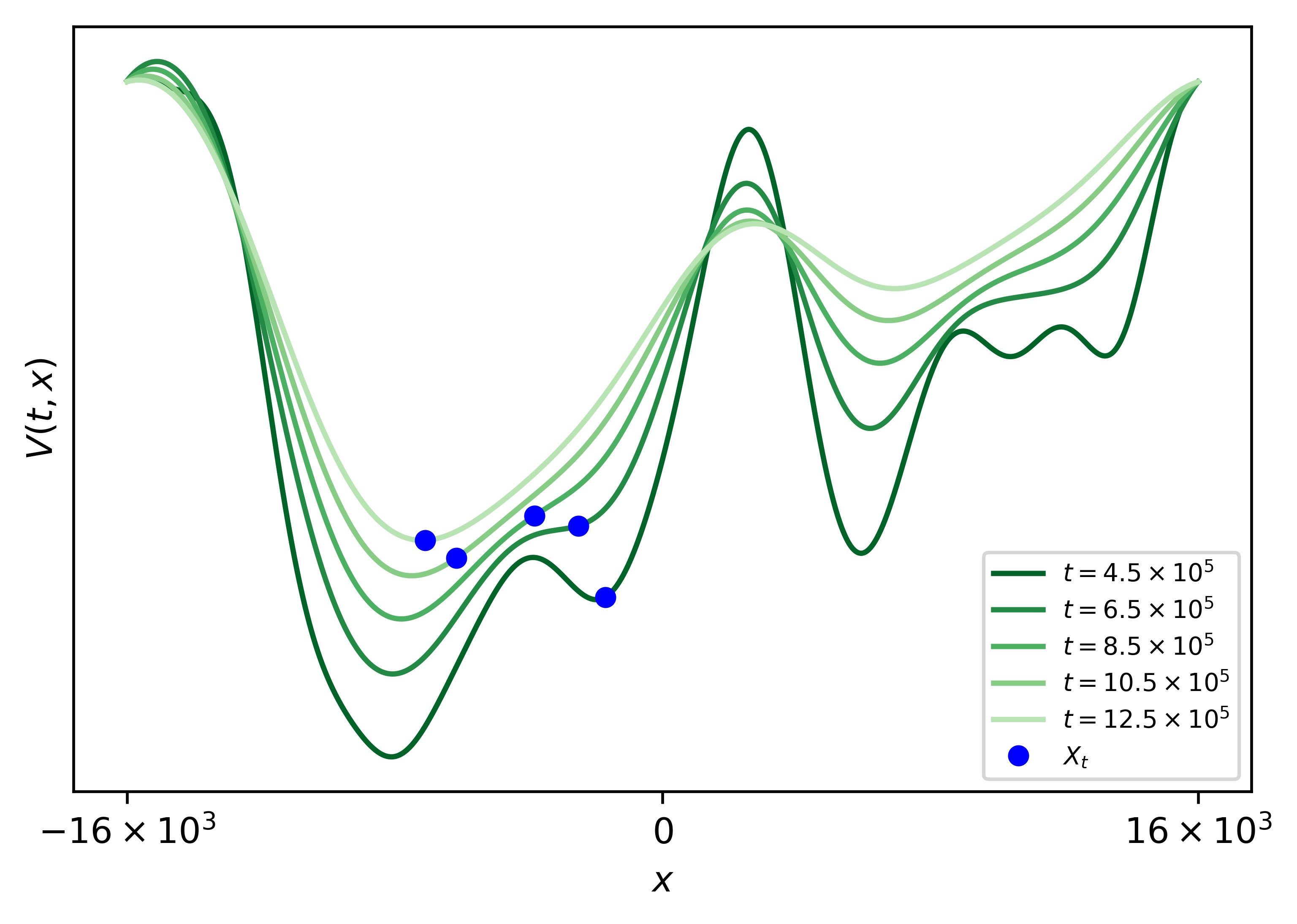
Figure 1. The process $X$ and the potential $V$ at different times. In the long run, the particle $X$ sticks most of the time to a local minimum of the potential $V$, as made precise in Theorem 5. For the numerical simulation used to generate this plot, we have assumed periodic boundary conditions and we have taken the initial condition $X_{t_{0}}=0$ with $t_{0}=4\times 10^{5}$.

We want to show two results on the behavior of $X$. The first one characterizes its short time behavior:

Theorem 2.

When the space of continuous function from $\mathbb{R}^{+}$ to $\mathbb{R}$ is endowed with the topology of uniform convergence on compact sets, the following convergence holds:

(2.5) $$\left(\frac{X_{\theta T}}{T^{3/4}}\right)_{\theta\geq 0}\;\xrightarrow[T\to 0]{(law)}\;\left(\int_{0}^{\theta}u(s,0)\text{\rm d}s\right)_{\theta\geq 0}.$$

We need to introduce some preliminary material to formulate our second result, dealing with the long time behavior of $X$. Some of the objects are illustrated on Fig. 2. Given $t>0$, let us define the set of zeros of the field $u$ at time $t$:

$$\mathcal{Z}_{t}\;=\;\{x\in\mathbb{R}:u(t,x)=0\}\,.$$

Let us distinguish attractive, or stable zeros, from repulsive, or unstable ones:

$$\begin{cases}\mathcal{Z}_{t}^{\mathrm{s}}\;=\;\{x\in\mathbb{R}:u(t,x)=0,\partial_{x}u(t,x)<0\}\,,\\ \mathcal{Z}_{t}^{\mathrm{u}}\;=\;\{x\in\mathbb{R}:u(t,x)=0,\partial_{x}u(t,x)>0\}.\end{cases}$$

We may also observe zeros that are nor stable nor unstable, say neutral:

$$\mathcal{Z}_{t}^{\mathrm{n}}\;=\;\{x\in\mathbb{R}:u(t,x)=0,\partial_{x}u(t,x)=0\}.$$

The next lemma allows to “trace back” a zero at time $t$ up to time $0$:

Lemma 1.

Almost surely, for all $t>0$ and all $x\in\mathcal{Z}_{t}^{\mathrm{s}}\cup\mathcal{Z}_{t}^{\mathrm{u}}$, there exists a unique continuous function $r_{(t,x)}:[0,t]\to\mathbb{R}$ such that for all $0<s\leq t$,

$$u(s,r_{(t,x)}(s))=0$$

and actually $r_{(t,x)}(s)\in\mathcal{Z}_{s}^{\mathrm{s}}$ if $x\in\mathcal{Z}_{s}^{\mathrm{s}}$ and $r_{(t,x)}(s)\in\mathcal{Z}_{s}^{\mathrm{u}}$ if $x\in\mathcal{Z}_{s}^{\mathrm{u}}$ (and thus in particular $\partial_{x}u(s,r_{(t,x)}(s))\neq 0$). The function $r_{(t,x)}$ is smooth on $]0,t[$ and for all $0<s\leq t$,

(2.6) $$\partial_{s}r_{(t,x)}(s)\;=\;-\frac{\partial_{s}u(s,r_{(t,x)}(s))}{\partial_{x}u(s,r_{(t,x)}(s))}\;=\;-\frac{\partial^{2}_{xx}u(s,r_{(t,x)}(s))}{\partial_{x}u(s,r_{(t,x)}(s))}.$$

Once properly rescaled, the long time behavior of $X$ is described by the limiting process $Z=(Z_{t})_{t\geq 0}$ introduced in the following proposition:

Proposition 3.

There exist unique processes $L=(L_{t})_{t\geq 0}$ and $R=(R_{t})_{t\geq 0}$ such that $L_{0}=R_{0}=0$ and, almost surely, for all $t>0$,

(2.7) $$\begin{cases}L_{t}\;=\;\max\{x\in\mathcal{Z}_{t}^{\mathrm{s}}\cup\mathcal{Z}_{t}^{\mathrm{u}}:r_{(t,x)}(0)<0\},\\ R_{t}\;=\;\min\{x\in\mathcal{Z}_{t}^{\mathrm{s}}\cup\mathcal{Z}_{t}^{\mathrm{u}}:r_{(t,x)}(0)>0\}.\end{cases}$$

Moreover, almost surely, for all $t>0$, one and only one of the following events occur

(2.8) $$\big{(}L_{t}\in\mathcal{Z}_{t}^{\mathrm{s}}\quad\text{and}\quad R_{t}\in\mathcal{Z}_{t}^{\mathrm{u}}\big{)}\qquad\text{or}\qquad\big{(}L_{t}\in\mathcal{Z}_{t}^{\mathrm{u}}\quad\text{and}\quad R_{t}\in\mathcal{Z}_{t}^{\mathrm{s}}\big{)}.$$

We can thus define a process $Z=(Z_{t})_{t\geq 0}$ by $Z_{0}=0$ and

$$\begin{cases}Z_{t}\;=\;L_{t}\quad\text{if}\quad L_{t}\in\mathcal{Z}_{t}^{\mathrm{s}}\\ Z_{t}\;=\;R_{t}\quad\text{if}\quad R_{t}\in\mathcal{Z}_{t}^{\mathrm{s}}\end{cases}$$

for $t>0$. The following properties of $Z$ hold:

1. Almost surely, $Z$ is càdlàg.

2. Almost surely, $Z$ is discontinuous at some time $t>0$ if and only if $Z_{t-}\in\mathcal{Z}^{\mathrm{n}}_{t}$.

3. Almost surely, for any compact interval $I\subset\mathbb{R}_{+}^{*}$, the number of discontinuities of $(Z_{t})_{t\in I}$ is finite and $(Z_{t})_{t\in I}$ is smooth away from the jumps.

4. $(Z_{t})_{t\geq 0}=(T^{-\frac{1}{2}}Z_{Tt})_{t\geq 0}$ in law for all $T>0$.

5. The variable $Z_{1}$ has a bounded density and there exists $c>0$ such that, for all $z\geq 0$,

$${c}\,\text{\rm e}^{-z/c}\;\leq\;\mathrm{P}(|Z_{1}|\geq z)\;\leq\;{\frac{1}{c}}\,\text{\rm e}^{-cz}.$$

Remark 4.

By a straightforward adaptation of the proof, items $1$ to $5$ above can be shown to hold as well with $L$ or $R$ in place of $Z$.

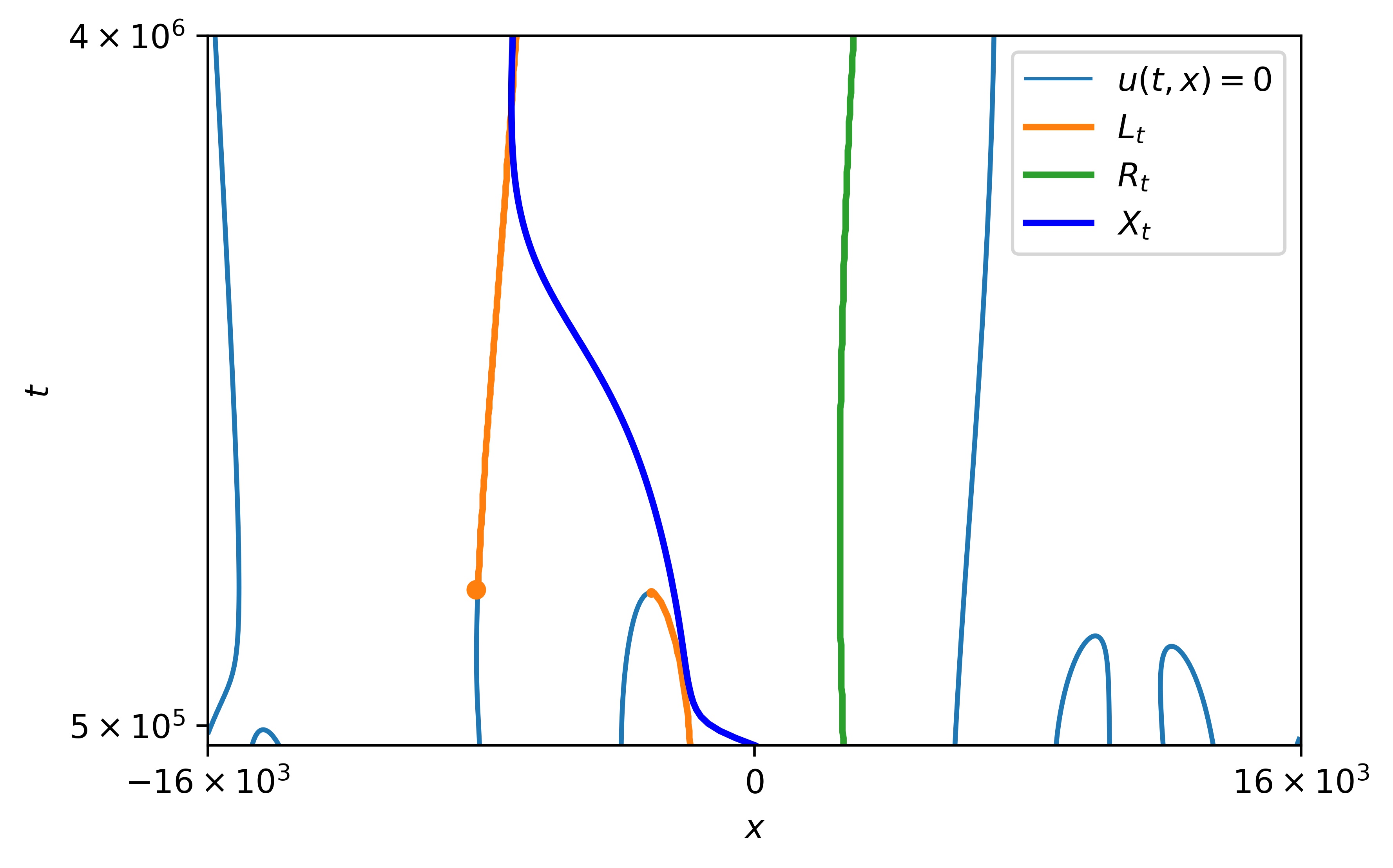
Figure 2. The processes $L$, $R$ and $X$, as well as the zeros of the velocity field $u$. The realization of the environment is the same as on Fig. 1.

We now come to our result on the long time behavior of $X$:

Theorem 5.

When the space of càdlàg function from $\mathbb{R}^{+}$ to $\mathbb{R}$ is endowed with the Skorokhod’s ${\mathcal{M}}_{1}$ topology for the convergence on compact sets, the following convergence holds:

(2.9) $$\frac{1}{T^{1/2}}\left(X_{\theta T}-Z_{\theta T}\right)_{\theta\geq 0}\;\xrightarrow[T\to+\infty]{(probability)}\;0$$

and thus in particular, by the scaling relation in item 4. in Proposition 3,

(2.10) $$\left(\frac{X_{\theta T}}{T^{1/2}}\right)_{\theta\geq 0}\;\xrightarrow[T\to+\infty]{(law)}\;(Z_{\theta})_{\theta\geq 0}.$$

Remark 6.

Since the process $(X_{\theta T})_{\theta\geq 0}$ is continuous and the process $(Z_{\theta T})_{\theta\geq 0}$ has jumps, it is not possible to obtain the convergence in the Skorokhod’s ${\mathcal{J}}$ topology. Let us remind the definition of the ${\mathcal{M}}_{1}$ topology, see [24]. Let $D([0,1],\mathbb{R})$ be the space of real càdlàg functions on $[0,1]$. For $f\in D([0,1],\mathbb{R})$, the completed graph of $f$ is defined as

$$\mathcal{G}(f)\;=\;\{(t,x)\in[0,1]\times\mathbb{R}:x\in[f(t-)\wedge f(t),f(t-)\vee f(t)]\}$$

with $f(t-)=\lim_{s\to t,s<t}f(s)$. We define an order on $G(f)$ as follows

$$(t,x)\leq(s,y)\quad\Leftrightarrow\quad t<s\quad\text{or}\quad t=s\text{ and }|x-f(t-)|\leq|y-f(s-)|.$$

A parametrization of $\mathcal{G}(f)$ is defined to be a continuous map $\varphi:[0,1]\to\mathcal{G}(f)$ such that $\varphi(0)=(0,f(0))$, $\varphi(1)=(1,f(1))$ and $\varphi$ is non-decreasing for the above order. The set of parametrizations of $\mathcal{G}(f)$ is denoted $\Pi(f)$. The ${\mathcal{M}}_{1}$ distance between two elements of $D([0,1],\mathbb{R})$ is defined as

$$d_{{\mathcal{M}}_{1}}(f,g)\;=\;\inf_{\varphi\in\Pi(f),\psi\in\Pi(g)}\left\{\sup_{0\leq\tau\leq 1}|\varphi(\tau)-\psi(\tau)|_{\infty}\right\}$$

where $|(t,x)|_{\infty}=\max\{|t|,|x|\}$. The definition is completely analogous on any other compact interval of $\mathbb{R}$.

3. Description of the environment

We establish here several features of the environment $u$, that will be used throughout this text. We first show the scaling property (3.1) below that will, among other things, play a key role in establishing Theorem 5. Second, we construct a grid of space-time points such that $u$ keeps the same sign on some time interval around each of these points, see Proposition 7 below as well as the subsequent constructions. This grid allows to derive a priori bounds on the processes $X$, $L$, $R$ and $Z$, that depend only on the sign of the the velocity field $u$. Third, we obtain estimates on the supremum of $u$ and its derivatives, see Lemma 2 below. These estimates will be mainly needed in the proof of Proposition 1.

Scaling property. For any $\alpha>0$,

(3.1) $$(u(t,x))_{t,x}\;\stackrel{{\scriptstyle(law)}}{{=}}\;(\alpha^{1/4}u(\alpha t,\alpha^{1/2}x))_{t,x}.$$

Indeed, both fields are Gaussian, centered and have the same covariance and, from the representation of the field $u$ in (2.3), we compute

(3.2) $$\mathrm{E}(u(t,x)u(s,y))\;=\;\int_{\mathbb{R}}P_{t}(x-z)P_{s}(z-y)\text{\rm d}z\;=\;P_{t+s}(x-y),$$

and $\alpha^{1/2}P_{\alpha(t+s)}(\alpha^{1/2}(x-y))=P_{t+s}(x-y)$ from (2.2).

Sign of the field $u$. Given $\ell>0$, let

(3.3) $$D(\ell)\;=\;\{\exists y:|y|\leq\ell/2\text{ and }\forall s\in[1/2,1],u(s,y)>0\}.$$

The following proposition provides a control on the probability of $D(\ell)$:

Proposition 7.

There exists $C>0$ such that, for all $\ell>0$,

$$\mathrm{P}\left(\overline{D(\ell)}\right)\;\leq\;\frac{1}{C}\text{\rm e}^{-C\ell}.$$

Remark 8.

By symmetry of $u$, by translation invariance and by the scaling property (3.1), we deduce from the above proposition that there exists $C>0$ such that, for any $x\in\mathbb{R}$ and any $t>0$,

$$\mathrm{P}\left(\overline{\{\exists y:|y-x|\leq\ell\sqrt{t}/2\text{ and }\forall s\in[t/2,t],\pm u(s,y)>0\}}\right)\;\leq\;\frac{1}{C}\text{\rm e}^{-C\ell}.$$

Proof.

We divide the proof into several steps.

1. Given a compact interval $I\subset\mathbb{R}$ and some $\alpha>0$,

(3.4) $$\mathrm{P}\left(\sup\left\{\int_{I}\varphi(x)\text{\rm d}B(x),\varphi\in{\mathcal{C}}^{1}(I),\|\varphi\|_{{\mathcal{C}}^{1}}\leq 1\right\}>\alpha\right)\;\leq\;\frac{1+2|I|^{3/2}}{\alpha}$$

with $\|\varphi\|_{{\mathcal{C}}^{1}}=\max_{x\in I}\{|\varphi(x)|+|\varphi^{\prime}(x)|\}$.

Indeed, let $I=[a,b]$ be some compact interval, and let $\varphi\in{\mathcal{C}}^{1}(I)$. An integration by parts yields

$$\int_{I}\varphi(x)\text{\rm d}B(x)\;=\;\varphi(b)(B(b)-B(a))-\int_{I}\varphi^{\prime}(x)(B(x)-B(a))\text{\rm d}x.$$

Hence,

$$\sup_{\varphi:\|\varphi\|_{{\mathcal{C}}^{1}}\leq 1}\int_{I}\varphi(x)\text{\rm d}B(x)\;\leq\;|B(b)-B(a)|+\int_{I}|B(x)-B(a)|\text{\rm d}x$$

and, by Markov inequality, for any $\alpha>0$,

$$\mathrm{P}\left(\sup_{\varphi:\|\varphi\|_{{\mathcal{C}}^{1}}\leq 1}\int_{I}\varphi(x)\text{\rm d}B(x)\;>\;\alpha\right)\; \leq\;\frac{1}{\alpha}\mathrm{E}\left(|B(b)-B(a)|+\int_{I}|B(x)-B(a)|\text{\rm d}x\right)$$

$$\leq\;\frac{1+2(b-a)^{3/2}}{\alpha}.$$

2. We introduce some definitions and notations. Let $\ell_{\star}\geq 1$. For $k\in\mathbb{Z}$, we define the points $x_{k}=k\ell_{\star}$ and the intervals

$$I_{k}\;=\;\left[x_{k}-\ell_{\star}/2,x_{k}+\ell_{\star}/2\right]\,,$$

as well as the variables

$$h_{k}\;=\;\frac{1}{\ell_{\star}^{3/2}}\sup\left\{\int_{I_{k}}\varphi(x)\text{\rm d}B(x),\;\varphi\in{\mathcal{C}}^{1}(I_{k}),\|\varphi\|_{{\mathcal{C}}^{1}}\leq 1\right\}.$$

Let also $n_{0}\in\mathbb{N}^{*}$ and let us define the variables

$$H_{k}\;=\;0\vee\left\lfloor\frac{\ln h_{k}}{n_{0}}\right\rfloor.$$

We observe that, by (3.4), $\mathrm{P}(H_{k}=0)$ goes to $1$ as $n_{0}$ goes to infinity, uniformly in $\ell_{\star}$.

3. Given $k\in\mathbb{Z}$ and $t>0$, let us define

$$\widetilde{u}(t,x_{k})\;=\;-\int_{I_{k}}P_{t}(x_{k}-y)\text{\rm d}B(y).$$

We want to control the difference between $\widetilde{u}(t,x_{k})$ and $u(t,x_{k})$. For this, let us introduce the variables

$$\eta_{k}\;=\;\left\{\begin{array}[]{ll}1&\text{if}\;\;H_{k-j}\leq|k-j|\;\quad\forall j\in\mathbb{Z},\\ 0&\text{otherwise}\end{array}\right.$$

We claim that, given $n_{0}$, for all $\ell_{\star}$ large enough, and for all $k$ such that $\eta_{k}=1$,

(3.5) $$\sup_{1/2\leq t\leq 1}|u(t,x_{k})-\widetilde{u}(t,x_{k})|<1.$$

Let us show (3.5). By translation invariance, it suffices to consider the case $k=0$. For all $t>0$,

$$u(t,0)-\widetilde{u}(t,0)\;=\;-\sum_{j\in\mathbb{Z}\backslash\{0\}}\int_{I_{j}}P_{t}(y)\text{\rm d}B(y).$$

Since $\eta_{0}=1$, it holds that $h_{j}\leq\text{\rm e}^{|j|n_{0}}$ for all $j\in\mathbb{Z}\backslash\{0\}$. Moreover, there exist $C,c>0$ such that $\|-P_{t}(\cdot)\|_{{\mathcal{C}}^{1}(I_{j})}\leq C\text{\rm e}^{-c|j|^{2}\ell_{\star}^{2}}$ for all $j\in\mathbb{Z}$, so that we finally obtain

$$\sup_{1/2\leq t\leq 1}|u(t,0)-\widetilde{u}(t,0)|\;\leq\;\sum_{j\in\mathbb{Z}\backslash\{0\}}C\ell_{\star}^{3/2}\text{\rm e}^{-c|j|^{2}\ell_{\star}^{2}}\text{\rm e}^{|j|n_{0}},$$

and this becomes smaller than $1$ for $\ell_{\star}$ large enough.

4. For all $n_{0}$ large enough, for all $\ell_{\star}\geq 1$, and for all $N\in\mathbb{N}$,

(3.6) $$\mathrm{P}(|\eta^{N}|_{1}<N)\;\leq\;\text{\rm e}^{-N},$$

where $\eta^{N}=(\eta_{-N},\dots,\eta_{N})$ and $|\eta^{N}|_{1}=\sum_{k=-N}^{N}\eta_{k}$.

Indeed, on the event

$$E_{N}\;=\;\{H_{j}\leq\left|\ |j|-N\ \right|\text{ for all }|j|>2N\},$$

it holds that

$$\{k\in\mathbb{Z}:|k|\leq N,\eta_{k}=0\}\;\subset\;\bigcup_{-2N\leq j\leq 2N}\{j-(H_{j}-1),\cdots,j+(H_{j}-1)\}$$

with the convention $\{a,\cdots,b\}=\emptyset$ if $b<a$. Therefore

$$|\{k\in\mathbb{Z}:|k|\leq N,\eta_{k}=0\}|\;\leq\;\sum_{-2N\leq j\leq 2N}\left[(2H_{j}-1)\vee 0\right]\;\leq\;\sum_{-2N\leq j\leq 2N}2H_{j}.$$

We thus obtain

(3.7) $$\mathrm{P}(|\eta^{N}|_{1}<N)\;\leq\;\mathrm{P}(\sum_{-2N\leq j\leq 2N}2H_{j}>N+1)+\mathrm{P}(\overline{E_{N}}).$$

For the second term, since by (3.4), for any $n\in\mathbb{N}$, $\mathrm{P}(H_{j}\geq n)\leq 3\text{\rm e}^{-n_{0}n}$ it holds that for $n_{0}$ large enough and all $N\geq 1$,

(3.8) $$\mathrm{P}(\overline{E_{N}})\;\leq\;\sum_{|j|>2N}\mathrm{P}(H_{j}>\left||j|-N\right|)\;\leq\;\frac{1}{2}\text{\rm e}^{-N}.$$

For the first one, as the variables $(H_{j})_{j\in\mathbb{Z}}$ are i.i.d., we obtain

(3.9) $$\mathrm{P}(\sum_{-2N\leq j\leq 2N}2H_{j}>N+1)\;\leq\;\text{\rm e}^{-2(N+1)}\mathrm{E}\left(\text{\rm e}^{4H_{0}}\right)^{4N+1}.$$

Finally, using once again that for any $n\in\mathbb{N}$, $\mathrm{P}(H_{j}\geq n)\leq 3\text{\rm e}^{-n_{0}n}$, one can choose $n_{0}$ large enough so that for all $N\geq 1$, the last term in (3.9) is smaller that $\text{\rm e}^{-N}/2$. Inserting (3.8) and (3.9) into (3.7) yields the result.

5. There exists $p>0$ such that, for all $\ell_{\star}\geq 1$ and for all $k\in\mathbb{Z}$,

(3.10) $$\mathrm{P}\left(\inf_{1/2\leq t\leq 1}\widetilde{u}(t,x_{k})\;>\;1\right)\;=\;p.$$

Again, to show this, it suffices to consider the case $k=0$. We observe that, almost surely, $\inf_{1/2\leq t\leq 1}\widetilde{u}(t,0)$ is a continuous function of $\ell_{\star}$, converging to $\inf_{1/2\leq t\leq 1}u(t,0)$ as $\ell_{\star}\to\infty$. Therefore, it is enough to establish the result for any fixed $\ell_{\star}\geq 1$ and for $u$ instead of $\widetilde{u}$. This last case can be handled with exactly the same proof, and we let $\ell_{\star}\geq 1$. Since the variables $(\widetilde{u}(t,0))_{t>0}$ are positively correlated, for any $0<a<b$, it holds that

$$\mathrm{P}\left(\inf_{t\in[a,b]}\widetilde{u}(t,0)\;>\;1/2\right)\\ \;\geq\;\mathrm{P}\left(\inf_{t\in[a,(a+b)/2]}\widetilde{u}(t,0)\;>\;1/2\right)\mathrm{P}\left(\inf_{t\in[(a+b)/2,b]}\widetilde{u}(t,0)\;>\;1/2\right).$$

Let us assume that $\mathrm{P}\left(\inf_{1/2\leq t\leq 1}\widetilde{u}(t,0)>1/2\right)=0$. By the above property, we find a sequence of nested closed intervals $(I_{n})_{n\geq 1}$ with $I_{1}=[1/2,1]$ and $|I_{n}|=2^{-n}$ such that, for all $n\geq 1$, $\mathrm{P}\left(\inf_{t\in I_{n}}\widetilde{u}(t,0)>1/2\right)=0$. Let $t_{0}\in\cap_{n\geq 1}I_{n}$. Since $\widetilde{u}(\cdot,0)$ is continuous almost surely in $t_{0}$,

$$\{\widetilde{u}(t_{0},0)>1/2\}\;\stackrel{{\scriptstyle a.s.}}{{=}}\;\bigcup_{n\geq 1}\{\widetilde{u}(t,0)>1/2,t\in I_{n}\},$$

and thus $\mathrm{P}(\widetilde{u}(t_{0},0)>1/2)=0$. This is a contradiction.

6. We start now the proof of the proposition itself. Let $p$ be the constant featuring in (3.10), let $n_{0}$ be large enough so that, for all $\ell_{\star}\geq 1$, $\mathrm{P}(H_{0})\geq 1-p/2$ and such that (3.6) holds, and finally let $\ell_{\star}$ be large enough so that (3.5) holds.

Let $N\in\mathbb{N}^{*}$, and let $\ell=(2N+1)\ell_{\star}$. Since the events $D(\ell)$ are increasing with $\ell$, it suffices to show the proposition for $\ell$ of this type. We start with

$$\mathrm{P}\left(\overline{D(\ell)}\right)\; \leq\;\mathrm{P}\left(\inf_{1/2\leq t\leq 1}u(t,x)\;\leq\;0,\ \forall x\in[-\ell/2,\ell/2]\right)$$

(3.11) $$\leq\;\mathrm{P}\left(\bigcap_{-N\leq i\leq N}\left\{\inf_{1/2\leq t\leq 1}u(t,x_{i})\;\leq\;0\right\}\right).$$

Let us denote by $A$ the event featuring in the right hand side of this last expression. From (3.6), we obtain

(3.12) $$\mathrm{P}(A)\;\leq\;\sum_{\stackrel{{\scriptstyle\sigma\in\{0,1\}^{2N+1},}}{{|\sigma|_{1}\geq N}}}\mathrm{P}(A\;|\;\eta^{N}=\sigma)\mathrm{P}(\eta^{N}=\sigma)\;+\;\text{\rm e}^{-N}.$$

Moreover from (3.5), we deduce that for all $i\in\mathbb{Z}$,

$$\left\{\inf_{1/2\leq t\leq 1}u(t,x_{i})\;\leq\;0\right\}\cap\{\eta(i)=1\}\;\subset\;\left\{\inf_{1/2\leq t\leq 1}\widetilde{u}(t,x_{i})\;\leq\;1\right\}.$$

Given $\sigma$ such that $|\sigma|_{1}\geq N$, we define $-N\leq i_{1}<\cdots<i_{N}\leq N$ to be the $N$ distinct smallest indexes such that for all $1\leq j\leq N$, $\eta_{i_{j}}=1$. We denote by $J$ the complementary set of the $(i_{k})_{1\leq k\leq N}$ in $\mathbb{Z}$. The event $\{\eta^{N}=\sigma\}$ can be written as

$$\left(\bigcap_{1\leq k\leq N}\{H_{i_{k}}=0\}\right)\cap\{(H_{j})_{j\in J}\in B\}$$

with $B$ some suitable event in $\mathbb{N}^{J}$. Therefore, as the $(H_{j})_{j\in\mathbb{Z}}$ are i.i.d., we obtain

$$\mathrm{P}(A|\eta^{N}=\sigma)\;\leq\;\prod_{k=1}^{N}\mathrm{P}\left(\inf_{1/2\leq t\leq 1}\widetilde{u}(t,x_{i_{k}})\;\leq\;1\Big{|}H_{i_{k}}=0\right)\;\leq\;\left(\frac{1-p}{1-p/2}\right)^{N},$$

and the proof follows by inserting this bound into (3.12). ∎

In the following we make use of Proposition 7 to give a property of the environment that we will use repeatedly till the end of the article. Let $K\geq 1$ be a constant that will be fixed below. Given $k\geq 0$ and $\alpha\geq 1$, we define a finite family of space-time boxes covering $B(k,\alpha)=[0,2^{k}]\times\left[-K\alpha\sqrt{2^{k}},+K\alpha\sqrt{2^{k}}\right]$ in the following way: For all $n\geq 0$, we define

$$t_{n}(k)=2^{k-n}\quad\text{ and }\quad\ell_{n}(k,\alpha)=(\alpha+n^{2})\sqrt{t_{n}(k)},$$

and also the space intervals

$$I_{n,j}(k,\alpha)=\left[j\ell_{n}(k,\alpha),(j+1)\ell_{n}(k,\alpha)\right],\quad j\in\mathbb{Z}.$$

We note $J_{n}(k,\alpha)$ the set of $j$ such that $I_{n,j}(k,\alpha)$ intersects $[-K\alpha\sqrt{2^{k}},K\alpha\sqrt{2^{k}}]$, so that $B(k,\alpha)$ is covered by the family of boxes $[t_{n+1}(k,\alpha),t_{n}(k,\alpha)]\times I_{n,j}(k,\alpha)$, for $n\geq 0$ and $j\in J_{n}(k,\alpha)$.

From now on we fix $K$ large enough so that for all $\alpha\geq 1$ and $k\geq 0$,

(3.13) $$\sum_{n\geq 0}2\ell_{n}(k,\alpha)\;\leq\;\frac{K}{3}\alpha\sqrt{t_{0}(k)}.$$

The reason for defining $K$ in this way will become clear later. For all $n\geq 0$ and $j\in J_{n}(k,\alpha)$, we consider the event

$$E_{n,j}(k,\alpha)\;=\;\{\exists y_{1},y_{2}\in I_{n,j}(k,\alpha):\ \forall s\in[t_{n+1}(k,\alpha),t_{n}(k{,\alpha})],u(s,y_{1})>0\text{ and }u(s,y_{2})<0\}.$$

and we define

(3.14) $$G(k,\alpha)\;=\;\bigcap_{n\geq 0,j\in J_{n}(k,\alpha)}E_{n,j}(k,\alpha).$$

We note that, uniformly in $\alpha$ and $k$,

$$\lfloor(2K)\ 2^{n/2}/(1+n^{2})\rfloor\;\leq\;|J_{n}(k,\alpha)|\;\leq\;(2K)\ 2^{n/2}.$$

Hence, by Remark 8,

(3.15) $$\mathrm{P}\left(\overline{G(k,\alpha)}\right)\;\leq\;\sum_{n\geq 0}(2K)2^{n/2}\frac{1}{C}\text{\rm e}^{-C(\alpha+n^{2})}$$

and, by Borel Cantelli lemma, we deduce that

(3.16) $$\text{almost surely for all }k\geq 1\text{ there exists }\alpha_{k}\geq 1\text{ so that }u\in G(k,\alpha_{k}).$$

This last property we be useful in many of the following proofs. A first consequence is the following

Remark 9.

An easy consequence of (3.16) is that almost surely, for any $i\in\mathbb{Z}$, the set $P_{i}=\{y\in\mathbb{R}:\forall s\in[2^{i-1},2^{i}],u(s,y)>0\}$ is (infinite and) not bounded. Indeed almost surely, $u\in G(k,\alpha_{k})$ for all $k\geq i$ so that there are at least $|J_{k-i}(k,\alpha_{k})|$ points in $P_{i}$ separated by a distance at least $\sqrt{2^{i}}$. As $|J_{k-i}(k,\alpha_{k})|$ goes to infinity when $k\to\infty$, this yields the result. The same result holds of course for the set $N_{i}=\{y\in\mathbb{R}:\forall s\in[2^{i-1},2^{i}],u(s,y)<0\}$.

Expected size of $u$ and its derivatives. We prove here some quantitative estimates on the field $u$ and its derivatives.

Lemma 2.

For any $\varepsilon>0$, there exists $C>0$ such that

(3.17) $$\mathrm{E}\left(\sup\left\{t^{\frac{1}{4}+\varepsilon}u(t,x)\,:\,t\in]0,1],x\in[-1,1]\right\}\right)\; \leq\;C,$$

(3.18) $$\mathrm{E}\left(\sup\left\{t^{\frac{3}{4}+\varepsilon}\partial_{x}u(t,x)\,:\,t\in]0,1],x\in[-1,1]\right\}\right)\; \leq\;C,$$

(3.19) $$\mathrm{E}\left(\sup\left\{t^{\frac{5}{4}+\varepsilon}\partial_{t}u(t,x)\,:\,t\in]0,1],x\in[-1,1]\right\}\right)\; \leq\;C.$$

As the field $u\stackrel{{\scriptstyle(law)}}{{=}}-u$, similar estimates hold for the infimum instead of the supremum.

Remark 10.

We stress that the result is false if $\varepsilon=0$ as these supremum are infinite almost surely in this case. Indeed, let us consider for example the field $u$. First, for all $t>0$ and $x\in\mathbb{R}$, the variables $t^{1/4}u(t,x)$ are identically distributed joint Gaussian variables. Second, given any $n\geq 1$ and points $x_{1},\dots,x_{n}$ with $-1\leq x_{1}<\dots<x_{n}\leq 1$, the Gaussian vector $(t^{1/2}u(t,x_{1}),\dots,t^{1/2}u(t,x_{n}))$ becomes uncorrelated as $t\to 0$. From this, one concludes that $\sup_{t\in]0,1],x\in[-1,1]}t^{1/4}u(t,x)=+\infty$ almost surely.

Proof.

Before starting the proof, we remind that we have already obtained the expression $\mathrm{E}(u(t,x)u(s,y))=P_{t+s}(x-y)$ in (3.2). Analogously, we derive

$$\partial_{x}u(t,x)=-\partial_{x}\int_{\mathbb{R}}P_{t}(x-y)\text{\rm d}B_{y}=-\int_{\mathbb{R}}P_{t}^{\prime}(x-y)\text{\rm d}B_{y}$$

and thus

$$\mathrm{E}(\partial_{x}u(t,x)\partial_{x}u(s,y))\; =\;\int_{\mathbb{R}}P_{t}^{\prime}(x-z)P_{s}^{\prime}(y-z)\text{\rm d}z\;=\;\partial_{x}\partial_{y}P_{t+s}(x-y)$$

(3.20) $$=\;-\partial_{xx}P_{t+s}(x-y),$$

as well as

$$\mathrm{E}(\partial_{t}u(t,x)\partial_{t}u(s,y))=\partial^{4}_{x}P_{t+s}(x-y).$$

The Lemma follows from Dudley’s theorem, see e.g. [19]. Let us show (3.17). We define a metric $d$ on $]0,1]\times[-1,1]$ by

(3.21) $$d((t,x),(s,y))\;=\;\left(\mathrm{E}\left(t^{\frac{1}{4}+\varepsilon}u(t,x)-s^{\frac{1}{4}+\varepsilon}u(s,y)\right)^{2}\right)^{\frac{1}{2}}.$$

Given $\delta>0$, let $N(\delta)$ be the minimal number of balls of radius $\delta$ for the metric $d$ needed to cover $]0,1]\times[-1,1]$. Dudley’s theorem asserts that

(3.22) $$\mathrm{E}\left(\sup\left\{t^{\frac{1}{4}+\varepsilon}u(t,x)\,:\,t\in]0,1],x\in[-1,1]\right\}\right)\;\leq\;24\int_{0}^{\infty}(\ln N(\delta))^{\frac{1}{2}}\text{\rm d}\delta.$$

Given $\delta>0$, let us derive a bound on $N(\delta)$. From (3.2) and (3.21), we compute

(3.23) $$d((t,x),(s,y))^{2}\;=\;(4\pi)^{-\frac{1}{2}}\left(t^{2\varepsilon}+s^{2\varepsilon}-2s^{\frac{1}{4}+\varepsilon}t^{\frac{1}{4}+\varepsilon}\left(\frac{s+t}{2}\right)^{-\frac{1}{2}}\text{\rm e}^{-\frac{(x-y)^{2}}{2(t+s)}}\right).$$

Hence the bounds

(3.24) $$d((t,x),(s,y))\;\leq\;(4\pi)^{-\frac{1}{4}}(t^{2\varepsilon}+s^{2\varepsilon})^{\frac{1}{2}}\;\leq\;(4\pi)^{-\frac{1}{4}}\sqrt{2}.$$

Therefore $N(\delta)=1$ as soon as $\delta\geq(4\pi)^{-\frac{1}{4}}\sqrt{2}$. Let us thus assume that $0<\delta<(4\pi)^{-\frac{1}{4}}\sqrt{2}$. It follows from (3.24) that the set

$$B_{0}\;=\;\left]0,c\,\delta^{\frac{1}{\varepsilon}}\right]\times[-1,1]\quad\text{with}\quad c\;=\;\pi^{\frac{1}{4\varepsilon}}$$

is contained in single ball of radius $\delta$. On $(]0,1]\times[-1,1])\backslash B_{0}$, we will show that there exists $C>0$ such that

(3.25) $$d((t,x),(s,y))\;\leq\;C\delta^{-\frac{1}{2\varepsilon}}\left(|t-s|+|x-y|\right).$$

This implies that there exists $C>0$ such that $N(\delta)\leq C\delta^{-2\left(1+\frac{1}{2\varepsilon}\right)}$, hence that the integral in (3.22) converges (to a value that depends on $\varepsilon$).

Let us show (3.25). By the triangle inequality, it holds that

$$d((t,x),(s,y))\;\leq\;d((t,x),(t,y))+d((t,y),(s,y)).$$

First, from (3.23),

$$d((t,x),(t,y))^{2}\;=\;\pi^{-\frac{1}{2}}t^{2\varepsilon}\left(1-\text{\rm e}^{-\frac{(x-y)^{2}}{4t}}\right)\;\leq\;C\frac{(x-y)^{2}}{t}\;\leq\;C\delta^{-\frac{1}{\varepsilon}}(x-y)^{2}$$

where we have used the bounds $t\leq 1$ and $1-\text{\rm e}^{-z}\leq z$ for all $z\geq 0$ to obtain the first inequality, and $t>c\delta^{\frac{1}{\varepsilon}}$ to get the second one. Next, from (3.23) again,

$$d((t,y),(s,y))^{2}\; =\;(4\pi)^{-\frac{1}{2}}t^{2\varepsilon}\left(1+\left(1+\frac{s-t}{t}\right)^{2\varepsilon}-2\left(1+\frac{s-t}{t}\right)^{\frac{1}{4}+\varepsilon}\left(1+\frac{s-t}{2t}\right)^{-\frac{1}{2}}\right)$$

$$=:\;t^{2\varepsilon}\varphi\left(\frac{s-t}{t}\right)\;\leq\;C\left(\frac{s-t}{t}\right)^{2}\;\leq\;C\delta^{-\frac{1}{\varepsilon}}(t-s)^{2}$$

where the first inequality follows from the fact that the distance $d$ is bounded by (3.24) and that $\varphi(0)=\varphi^{\prime}(0)=0$, and where the second one is obtained thanks to the bound $t>c\delta^{\frac{1}{\varepsilon}}$.

The proof of (3.18) is analogous and we only outline the main steps. This time,

$$d((t,x),(s,y))^{2}\;=\;(16\pi)^{-\frac{1}{2}}\left(t^{2\varepsilon}+s^{2\varepsilon}-2s^{\frac{3}{4}+\varepsilon}t^{\frac{3}{4}+\varepsilon}\left(\frac{s+t}{2}\right)^{-\frac{3}{2}}\left(1-\frac{(x-y)^{2}}{t+s}\right)\text{\rm e}^{-\frac{(x-y)^{2}}{2(t+s)}}\right).$$

Since the function $z\mapsto(1-z^{2})\text{\rm e}^{-z^{2}/2}$ is bounded, we obtain a bound analogous to (3.24):

$$d((t,x),(s,y))\;\leq\;C(t^{2\varepsilon}+s^{2\varepsilon})^{\frac{1}{2}}\;\leq\;C.$$

Hence, again, it is enough to show (3.25) for $t>c\delta^{\frac{1}{\varepsilon}}$ for some $c>0$, and the rest of the proof uses only completely similar computations.

The proof of (3.19) is analogous. ∎

4. Proof of Proposition 1 and Theorem 2

Proof of Proposition 1.

Let us first show that, almost surely, there exists $\varepsilon>0$ so that $(X_{t})_{0\leq t\leq\varepsilon}$ is defined as the fixed point of the map

$$\Phi\;:\;{\mathcal{C}}\left([0,\varepsilon],[-1,1]\right)\to{\mathcal{C}}\left([0,\varepsilon],[-1,1]\right),\quad f\mapsto\Phi(f)=t\mapsto\int_{0}^{t}u(s,f_{s})\text{\rm d}s.$$

First, if we choose $\varepsilon$ small enough, $\Phi$ is well defined. Indeed, thanks to Lemma 2, the time integral is a.s. convergent and moreover, taking for example $\delta=1/10$, we find $C>0$ such that, for all $f\in{\mathcal{C}}\left([0,\varepsilon],[-1,1]\right)$,

$$\|\Phi(f)\|_{\infty}\;\leq\;C\int_{0}^{\varepsilon}\frac{\text{\rm d}s}{s^{1/4+\delta}}\;\leq\;1$$

if $\varepsilon$ is chosen small enough.

Next, $\Phi$ is contracting if $\varepsilon$ is small enough. Indeed, there exists $C>0$ such that, for all $f,g\in{\mathcal{C}}\left([0,\varepsilon],[-1,1]\right)$,

$$\|f-g\|_{\infty} \;\leq\;\int_{0}^{\varepsilon}|u(s,f_{s})-u(s,g_{s})|\text{\rm d}s$$

$$\;\leq\;\|f-g\|_{\infty}\int_{0}^{\varepsilon}\sup_{x\in[-1,1]}|\partial_{x}u(s,x)|\text{\rm d}s\;\leq\;C\int_{0}^{\varepsilon}\frac{\text{\rm d}s}{s^{3/4+\delta}}\;\leq\;1$$

if $\varepsilon$ is chosen small enough.

It is thus almost surely possible to define $(X_{t})_{0\leq t\leq\varepsilon}$ as the unique fixed point of $\Phi$. Clearly this process is continuous and satisfies (2.4) for $0\leq t\leq\varepsilon$. Let us show that this process can be extended on $\mathbb{R}_{+}$.

We define $(X_{t})_{t\in I}$ as the maximal solution for the Cauchy problem $\partial_{t}X_{t}=u(t,X_{t})$ with the condition that, at time $t=\varepsilon$, $X_{t}$ coincides with $X_{\varepsilon}$ found above. We already know that $\inf I=0$ so that it remains to prove that $\sup I=+\infty$. If $t_{\star}=\sup I<\infty$ then, $(X_{t})_{0<t<t_{\star}}$ explodes before time $t_{\star}$, i.e. $\lim_{t\to t_{\star}^{-}}|X_{t}|=+\infty$. This is impossible thanks to Remark 9. Indeed, let $i$ be the integer such that $2^{i-1}<t_{\star}\leq 2^{i}$ and choose $x\in P_{i}$ and $y\in N_{i}$ so that $x<X_{2^{i-1}}<y$. This implies that $X_{s}\in]x,y[$ for all $2^{i-1}\leq s<t_{\star}$ and this is a contradiction. ∎

Proof of Theorem 2.

We fix some $\theta_{0}>0$. For $0<\theta\leq\theta_{0}$ and $T>0$, we decompose

$$\frac{X_{\theta T}}{T^{3/4}}\;=\;\frac{1}{T^{3/4}}\int_{0}^{\theta T}u(s,0)\text{\rm d}s\;+\;\frac{1}{T^{3/4}}\int_{0}^{\theta T}\big{(}u(s,X_{s})-u(s,0)\big{)}\text{\rm d}s.$$

Thanks to the scaling relation (3.1),

$$\left(\frac{1}{T^{3/4}}\int_{0}^{\theta T}u(s,0)\text{\rm d}s\right)_{0\leq\theta\leq\theta_{0}}\;=\;\left(\int_{0}^{\theta}u(s,0)\text{\rm d}s\right)_{0\leq\theta\leq\theta_{0}}\quad\text{in law}.$$

Hence, it is enough to show that almost surely

$$\sup_{0<\theta\leq\theta_{0}}\left|\frac{1}{T^{3/4}}\int_{0}^{\theta T}u(s,X_{s})-u(s,0)\ \text{\rm d}s\right|\;\to\;0\quad\text{as}\quad T\to 0.$$

Let $\delta=1/10$. Thanks to Lemma 2, almost surely, there exists a constant $C>0$ so that for all $0<t\leq 1$ and all $x\in[-1,1]$, we have the bounds $|t^{\frac{1}{4}+\delta}u(t,x)|<C$ and $|t^{\frac{3}{4}+\delta}\partial_{x}u(t,x)|<C$. From now on, by continuity, we take $T$ small enough so that $\theta_{0}T\leq 1$ and $\sup_{s\leq\theta_{0}T}|X_{s}|\leq 1$. It thus holds that for $0\leq t\leq\theta_{0}T$,

$$|X_{t}|\;\leq\;|\int_{0}^{t}u(s,X_{s})\ \text{\rm d}s|\;\leq\;\int_{0}^{t}\sup_{x\in[-1,1]}|u(s,x)|\ \text{\rm d}s\;\leq\;C\int_{0}^{t}\frac{\text{\rm d}s}{s^{1/4+\delta}}\;\leq\;2Ct^{3/4-\delta}.$$

Next, for all $0\leq\theta\leq\theta_{0}$,

$$\left|\frac{1}{T^{3/4}}\int_{0}^{\theta T}u(s,X_{s})-u(s,0)\text{\rm d}s\right| \;\leq\;\frac{1}{T^{3/4}}\int_{0}^{\theta T}|u(s,X_{s})-u(s,0)|\text{\rm d}s$$

$$\;\leq\;\frac{1}{T^{3/4}}\int_{0}^{\theta T}\sup_{x\in[-1,1]}|\partial_{x}u(s,x)||X_{s}|\text{\rm d}s$$

$$\;\leq\;\frac{2C^{2}}{T^{3/4}}\int_{0}^{\theta T}\frac{1}{s^{3/4+\delta}}s^{3/4-\delta}\text{\rm d}s\;\leq\;4C^{2}\frac{(\theta_{0}T)^{1-2\delta}}{T^{3/4}}$$

and the last bound (uniform on $0\leq\theta\leq\theta_{0}$) converges to $0$ as $T\to 0$. ∎

5. Proof of Lemma 1 and Proposition 3

We start with a Lemma, that guarantees that the zeros of $u$ are almost surely never degenerate, i.e. either $\partial_{x}u$ or $\partial_{t}u$ is non-zero whenever $u$ vanishes. This will enable us to invoke the implicit function theorem in several places. Moreover, we show also that there are only countably many isolated points where $\partial_{x}u$ vanishes, corresponding to the tops of the blue curves on Fig. 2. This is the key ingredient to show item 3 in Proposition 3.

Lemma 3.

The field $u$ satisfies

1. $\mathrm{P}\big{(}\exists(t,x)\in\mathbb{R}_{+}^{*}\times\mathbb{R}:u(t,x)=\partial_{t}u(t,x)=\partial_{x}u(t,x)=0\big{)}\;=\;0.$

2. Almost surely, on any compact set $K\subset\mathbb{R}_{+}^{*}\times\mathbb{R}$, the set of points where $u(t,x)=\partial_{x}u(t,x)=0$ is finite.

Remark 11.

As our proof shows, the first item holds actually for any smooth field $u$ such that $(u,\partial_{t}u,\partial_{x}u)$ has a locally bounded density around $0$.

Proof.

For the first item, let us consider the field $\varphi$ defined by

(5.1) $$\varphi(t,x)\;=\;\big{(}u(t,x),\partial_{t}u(t,x),\partial_{x}u(t,x)\big{)},\quad t>0,x\in\mathbb{R}.$$

From the scaling relation (3.1), we obtain also

(5.2) $$\big{(}\varphi(t,x)\big{)}_{t,x}\stackrel{{\scriptstyle(law)}}{{=}}\big{(}\alpha^{1/4}u(\alpha t,\alpha^{1/2}x),\alpha^{5/4}\partial_{t}u(\alpha t,\alpha^{1/2}x),\alpha^{3/4}\partial_{x}u(\alpha t,\alpha^{1/2}x)\big{)}_{t,x}.$$

By sigma additivity, together with the scaling relation (5.2) and the space translation invariance we find that it suffices to show that

$$\mathrm{P}\big{(}\exists(t,x)\in[1,2]\times[-1,1]:\varphi(t,x)=0\big{)}\;=\;0,$$

To prove this, let us first show that there exists some $C>0$ such that, for any $(t,x)\in[1,2]\times[-1,1]$ and for any $\varepsilon>0$,

(5.3) $$\mathrm{P}(|\varphi(t,x)|<\varepsilon)\;<\;C\varepsilon^{3}$$

where $|\cdot|$ denotes the Euclidian norm. First, since $t\leq 2$, by the scaling relation (5.2) and translation invariance, for all $(t,x)\in[1,2]\times[-1,1]$

$$\mathrm{P}(|\varphi(t,x)|<\varepsilon)\leq\mathrm{P}(|\varphi(2,0)|<\varepsilon).$$

Therefore, to show (5.3), since $\varphi(2,0)$ is Gaussian, it suffices to show that its covariance is non-degenerate, i.e. invertible. Since

$$\mathrm{E}(\varphi_{i}\varphi_{j})\;=\;\int_{\mathbb{R}}\partial^{i}P_{2}(z)\partial^{j}P_{2}(z)\text{\rm d}z$$

for $1\leq i,j\leq 3$, with the notation $(\partial^{1},\partial^{2},\partial^{3})=(1,\partial_{t},\partial_{x})$, and since $P_{2}(\cdot)$, $\partial_{t}P_{2}(\cdot)$ and $\partial_{x}P_{2}(\cdot)$ are linearly independent as elements of $L^{2}(\mathbb{R})$, the covariance is indeed non-degenerate.

Next, because $\varphi$ is smooth, it holds that

(5.4) $$\{\exists(t,x)\in[1,2]\times[-1,1]:\varphi(t,x)=0\}\;=\;\\ \bigcup_{N\in\mathbb{N}^{*}}\left\{\exists(t,x)\in[1,2]\times[-1,1]:\varphi(t,x)=0\text{ and }\|\varphi^{\prime}\|_{\infty}<N\right\}$$

with $\|f\|_{\infty}=\max_{(t,x)\in[1,2]\times[-1,1]}\|f(t,x)\|$ for any continuous function $f$ on $[1,2]\times[-1,1]$ with values in linear application from $\mathbb{R}^{2}$ to $\mathbb{R}^{3}$, and where $\|\cdot\|$ is the operator norm when both spaces are endowed with the euclidian norms. Thus it suffices to show that, for any $N\in\mathbb{N}^{*}$, the probability of the corresponding set in the union in the right hand side of (5.4) is zero. Let $N\in\mathbb{N}^{*}$, let $\varepsilon>0$ and let us define the points

$$(t_{i},x_{j})\;=\;\left(1+i\varepsilon,j\varepsilon\right),\quad i\in\mathbb{N},\;i<1/\varepsilon,\quad j\in\mathbb{Z},\;|j|<1/\varepsilon.$$

The number of such points is bounded by $2/\varepsilon^{2}$. Now, under the condition $\|\varphi^{\prime}\|_{\infty}<N$, if $\varphi(t,x)=0$ for some $(t,x)\in[1,2]\times[-1,1]$, then $|\varphi(t_{i},x_{j})|\leq\sqrt{2}\varepsilon N$ for one of the points $(t_{i},x_{j})$ at least. Hence, using (5.3), we obtain

$$\mathrm{P}\left(\exists(t,x)\in[1,2]\times[-1,1]:\varphi(t,x)=0\text{ and }\|\varphi^{\prime}\|_{\infty}<N\right)\; \leq\;\sum_{i,j}\mathrm{P}\left(|\varphi(t_{i},x_{j})|\leq\sqrt{2}\varepsilon N\right)$$

$$\leq\;\frac{2C}{\varepsilon^{2}}\left(\sqrt{2}\varepsilon N\right)^{3}.$$

Since $\varepsilon$ may be taken arbitrarily small for given $N\in\mathbb{N}^{*}$, the left hand side vanishes for any $N\in\mathbb{N}^{*}$.

We turn to the second item. As $K$ is compact it is enough to prove that the set of $(s,y)\in K$, so that $u(s,y)=\partial_{x}u(s,y)=0$, has only isolated points. Using item $1$, we may assume that almost surely for all points of this set $\partial_{t}u(s,y)\neq 0$. We consider one of these points, and using the implicit function theorem, we know that there exists a real function $S$ defined in a neighborhood of $y$ so that the set of zeros of the field $u$ coincides with the graph of this function on a neighborhood of $(s,y)$. The function $S$ satisfies

$$S^{\prime}(z)\; =\;-\frac{\partial_{x}u(S(z),z)}{\partial_{t}u(S(z),z)},$$

$$S^{\prime\prime}(z)\; =\;-1+S^{\prime}(z)\left(\frac{\partial_{x}u(S(z),z)\partial_{tt}u(S(z),z)}{(\partial_{t}u(S(z),z))^{2}}-2\frac{\partial_{tx}u(S(z),z)}{\partial_{t}u(S(z),z)}\right)$$

for $z$ in a neighborhood of $y$. Therefore, in a neighborhood of $y$, $\partial_{x}u(S(z),z)=0$ if and only if $S^{\prime}(z)=0$ and, since $S^{\prime}(y)=0$, we have $S^{\prime\prime}(z)<0$, and thus also $S^{\prime}(z)\neq 0$ for $z\neq y$. ∎

We have now all ingredients for the

Proof of Lemma 1.

By Lemma 3, one may assume that almost surely on every point $(s,y)$ such that $u(s,y)=0$, either $\partial_{t}u(s,y)\neq 0$ or $\partial_{x}u(s,y)\neq 0$. The main observation is that, if $(s,y)$ is such that $u(s,y)=0$ and $\partial_{x}u(s,y)=0$, then there exists $\varepsilon>0$ such that

(5.5) $$u(s^{\prime},y^{\prime})\neq 0\text{ for all }(s^{\prime},y^{\prime})\in]s,s+\varepsilon[\times]y-\varepsilon,y+\varepsilon[.$$

Indeed, as $\partial_{t}u(s,y)=\partial_{xx}u(s,y)\neq 0$, we may assume that $\partial_{t}u(s,y)>0$ (the other case being analogous). By continuity, there exists $\varepsilon>0$ such that $\partial_{t}u(s^{\prime},y^{\prime})>0$ for all $(s^{\prime},y^{\prime})\in]s,s+\varepsilon[\times]y-\varepsilon,y+\varepsilon[$, and $u(s,y^{\prime})\geq 0$ for all $y^{\prime}\in]y-\varepsilon,y+\varepsilon[$. Therefore $u(s^{\prime},y^{\prime})>u(s,y^{\prime})\geq 0$ or all $(s^{\prime},y^{\prime})\in]s,s+\varepsilon[\times]y-\varepsilon,y+\varepsilon[$, which shows the claim. Let now $t>0$ and $x\in{\mathcal{Z}}_{t}^{\mathrm{s}}\cup{\mathcal{Z}}_{t}^{\mathrm{u}}$. We consider the set

$${\mathcal{F}}\;=\;\left\{\begin{aligned} &0\leq s_{0}<t:\textrm{there exists a function }\ r_{(t,x)}:\;]s_{0},t]\to\mathbb{R},\textrm{ and}\\ &\textrm{ a neighbourhood }{\mathcal{V}}\ \textrm{ of }(t,x)\textrm{ containing the graph of }r_{(t,x)},\\ &\textrm{ such that}\textrm{ for all }(s,y)\in{\mathcal{V}},\ u(s,y)=0\Leftrightarrow y=r_{(t,x)}(s)\end{aligned}\right\}.$$

Since $\partial_{x}u(t,x)\neq 0$, the implicit function theorem guarantees that ${\mathcal{F}}\neq\emptyset$. Let

$$s_{min}\;=\;\inf{\mathcal{F}}$$

and let us prove by contradiction that $s_{min}=0$. Assume that $s_{min}>0$.

Remind the definition of $G(k,\alpha_{k})$ in (3.14) and also property (3.16). We choose $k$ large enough so that $t_{0}(k)=2^{k}\geq t$ and $|x|\leq\frac{K}{3}\alpha_{k}\sqrt{t_{0}(k)}$. Since $u\in G(k,\alpha_{k})$ and since the graph of $r_{(t,x)}$ does not intersect $\{u>0\}\cup\{u<0\}$, we obtain that for all $i\geq 0$, $|r_{(t,x)}(t_{i}(k))-r_{(t,x)}(t_{i+1}(k))|\leq 2\ell_{i}(k)$. Hence, by definition of $K$ in (3.13), for all $s_{min}\leq s\leq t$, $|r_{(t,x)}(s)|\leq\frac{2K}{3}\alpha_{k}\sqrt{t_{0}(k)}$, and the set $\{(s,r_{x}(s)):s_{min}<s\leq t\}$ is bounded. By compactness, there exists $y\in\mathbb{R}$ such that $(s_{min},y)$ lies in its closure. Therefore, by continuity, $u(s_{min},y)=0$ and, by the implicit function theorem again, $\partial_{x}u(s_{min},y)=0$ as otherwise one should have $\inf{\mathcal{F}}<s_{min}$. We reach a contradiction with (5.5).

Let us next show that $r_{(t,x)}$ is continuous in $0$. This is a consequence of the fact that $r_{(t,x)}$ satisfies Cauchy property as $s$ goes to $0$. Indeed, with the same argument as above, for all $j$ large enough and $0<s,s^{\prime}<t_{j}(k)$,

$$|r_{(t,x)}(s)-r_{(t,x)}(s^{\prime})|\;\leq\;\sum_{n\geq j}2\ell_{n}(k),$$

and this last sum goes to zero as $j\to+\infty$.

Finally, that stable zeros remain stable, and unstable ones remain unstable, follows from the fact that $\partial_{x}u(s,r_{(t,x)}(s))\neq 0$ for all $s\in]0,t]$, as the above argument shows. The expression (2.6) follows from the implicit function theorem. ∎

Proof of Proposition 3: existence of the processes $L$ and $R$ satisfying (2.7) and (2.8).

Let us first show that there exist processes $L$ and $R$ satisfying (2.7) almost surely for any $t>0$. To fix the ideas, let us deal with $L$. As, almost surely, $u(t,\cdot)$ is analytic for any $t>0$, ${\mathcal{Z}}_{t}$ has no accumulation points, and it is enough to prove that the set $\{x\in{\mathcal{Z}}_{t}^{\mathrm{s}}\cup{\mathcal{Z}}_{t}^{\mathrm{u}}:r_{(t,x)}(0)<0\}$ is non-empty and bounded above. Let us fix $t>0$ and show that, almost surely, for any $t^{\prime}\in]0,t]$, $\{x\in{\mathcal{Z}}_{t^{\prime}}^{\mathrm{s}}\cup{\mathcal{Z}}_{t^{\prime}}^{\mathrm{u}}:r_{(t^{\prime},x)}(0)<0\}$ is non-empty and bounded above.

We choose $k$ large enough so that $2^{k}\geq t$. Using Remark 9, almost surely, $u(t^{\prime},\cdot)$ changes sign infinitely many often on $]-\infty,-K\alpha_{k}\ \sqrt{2^{k}}[$. As $u$ is continuous, each interval where $u$ changes sign intersects ${\mathcal{Z}}_{t^{\prime}}$. One can actually say more as, from the first item in Lemma 3, we may assume that $\partial_{xx}u=\partial_{t}u\neq 0$ whenever $u=\partial_{x}u=0$ and thus, for all $y\in{\mathcal{Z}}_{t^{\prime}}^{\mathrm{n}}$, the function $u(t,\cdot)$ vanishes but does not change sign in a neighborhood of $y$. From this one deduces that each interval where $u$ changes sign intersects ${\mathcal{Z}}_{t^{\prime}}^{\mathrm{s}}\cup{\mathcal{Z}}_{t^{\prime}}^{\mathrm{u}}$ (we will use repeatedly this argument in the following).

Thus there exists $x\in]-\infty,-K\alpha_{k}\ \sqrt{2^{k}}[\cap({\mathcal{Z}}_{t^{\prime}}^{\mathrm{s}}\cup{\mathcal{Z}}_{t^{\prime}}^{\mathrm{u}})$. Arguing as in the proof of Lemma 1, we obtain that for all $0<s\leq t^{\prime}$, $r_{t^{\prime},x}(s)\leq-\frac{2K}{3}\alpha_{k}\sqrt{2^{k}}$ and in particular $r_{t^{\prime},x}(0)<0$. This implies that $\{x\in{\mathcal{Z}}_{t^{\prime}}^{\mathrm{s}}\cup{\mathcal{Z}}_{t^{\prime}}^{\mathrm{u}}:r_{(t^{\prime},x)}(0)<0\}$ is non-empty. Moreover it is also bounded above as, with the same argument, for $x\in{\mathcal{Z}}_{t^{\prime}}^{\mathrm{s}}\cup{\mathcal{Z}}_{t^{\prime}}^{\mathrm{u}}$ such that $x\geq K\alpha_{k}\ \sqrt{2^{k}}$, it holds that $r_{t^{\prime},x}(s)\geq\frac{2K}{3}\alpha_{k}\sqrt{2^{k}}>0$.

Second, let us show (2.8). For this, let us first prove that the probability of the event

(5.6) $${\mathcal{W}}\;=\;\{\exists(t,x)\in\mathbb{R}_{+}^{*}\times\mathbb{R}:r_{(t,x)}(0)=0\}$$

vanishes. Let us decompose this event as

$${\mathcal{W}}\;=\;\bigcup_{t>0}{\mathcal{W}}_{t}(0)\quad\text{with}\quad{\mathcal{W}}_{t}(y)\;=\;\{\exists x\in\mathbb{R}:r_{(t,x)}(0)=y\},\;y\in\mathbb{R}.$$

Since, by Lemma 1, the events ${\mathcal{W}}_{t}(0)$ increase as $t$ decreases, it is enough to show that $\mathrm{P}({\mathcal{W}}_{t}(0))=0$ for any $t>0$. Let $t>0$. As argued above, the set ${\mathcal{Z}}_{t}^{\mathrm{s}}\cup{\mathcal{Z}}_{t}^{\mathrm{u}}$ is almost surely unbounded above and below, and countable. Let us denote its elements by $(z_{k})_{k\in\mathbb{Z}}$, with $z_{k}<z_{k+1}$ for all $k\in\mathbb{Z}$ and $z_{0}=\min({\mathcal{Z}}_{t}^{\mathrm{s}}\cup{\mathcal{Z}}_{t}^{\mathrm{u}})\cap\mathbb{R}_{+}$. Therefore, given $y\in\mathbb{R}$, it holds that $\mathrm{P}({\mathcal{W}}_{t}(y))>0$ if and only if $\mathrm{P}(r_{(t,z_{k})}(0)=y)>0$ for some $k\in\mathbb{Z}$. Since the atoms of a random variable are at most countable, the set of $y\in\mathbb{R}$ such that $\mathrm{P}({\mathcal{W}}_{t}(y))>0$ is at most countable. As $\mathrm{P}({\mathcal{W}}_{t}(y))$ is constant in $y\in\mathbb{R}$ by translation invariance, we deduce that $\mathrm{P}({\mathcal{W}}_{t}(y))=0$ for all $y\in\mathbb{R}$.

On ${\mathcal{W}}^{c}$, let us assume by contradiction that there exists some $t>0$ such that $L_{t},R_{t}\in{\mathcal{Z}}_{t}^{\mathrm{s}}$ (one rules out analogously the case $L_{t},R_{t}\in{\mathcal{Z}}_{t}^{\mathrm{u}}$). Since $u(t,x)<0$ for $x>L_{t}$ in a neighborhood of $L_{t}$ and since $u(t,x)>0$ for $x<R_{t}$ in a neighborhood of $R_{t}$, we find that there exists $x\in Z_{t}^{\mathrm{u}}\cap]L_{t},R_{t}[$. By (2.7), we would have $r_{(t,x)}(0)=0$, but this is impossible if ${\mathcal{W}}^{c}$ is realized. ∎

Proof of item 1 in Proposition 3.

First, let us show that $Z$ is continuous in $t=0$. This follows from the fact that $L$ and $R$ are continuous in $t=0$. To fix the ideas, let us show this for $L$. We actually prove a bit more: For all $\varepsilon>0$, almost surely if $t>0$ is small enough, $|L_{t}|\leq t^{1/2-\varepsilon}$. Let $\varepsilon>0$. As, almost surely, $u\in G(0,\alpha_{0})$ and $r_{t,L_{t}}(0)<0$, arguing as in the proof of Lemma 1, we obtain that there exists $C>0$ such that, for all $0<t\leq 1$,

$$L_{t}\;\leq\;\sum_{n\geq\lfloor-\log_{2}t\rfloor}2\ell_{n}(0,\alpha_{0})\;=\;\sum_{n\geq\lfloor-\log_{2}t\rfloor}2(\alpha_{0}+n^{2})\sqrt{2^{-n}}\;\leq\;C(\log_{2}t)^{2}t^{1/2}.$$

Thus, for $t>0$ small enough, the upper bound $L_{t}\leq t^{1/2-\varepsilon}$ holds. Moreover, the above bound implies that for $t>0$ small enough,

$$t^{1/2-\varepsilon}-\sum_{n\geq\lfloor-\log_{2}t\rfloor}2\ell_{n}(0,\alpha_{0})\;\geq\;2\ell_{\lfloor-\log_{2}t\rfloor}(0,\alpha_{0}).$$

Therefore, the function $u(t,\cdot)$ changes sign in $[-t^{1/2-\varepsilon},-\sum_{n\geq\lfloor-\log_{2}t\rfloor}2\ell_{n}(0,\alpha_{0})[$ so that this interval intersects ${\mathcal{Z}}_{t}$. Using the same argument as in the proof of Lemma 1, one can even says that this interval intersects ${\mathcal{Z}}_{t}^{\mathrm{s}}\cup{\mathcal{Z}}_{t}^{\mathrm{u}}$ and we consider some $x$ in this intersection. As $u\in G(0,\alpha_{0})$, $r_{t,x}(0)\leq x+\sum_{n\geq\lfloor-\log_{2}t\rfloor}2\ell_{n}(0)<0$ and this implies that $L_{t}\geq x\geq-t^{1/2-\varepsilon}$.

Second, let $t>0$ and let us prove that $Z$ is càdlàg at $t$. Because $L_{t},R_{t}\in{\mathcal{Z}}_{t}^{\mathrm{s}}\cup{\mathcal{Z}}_{t}^{\mathrm{u}}$, the implicit function theorem implies that there exist $\varepsilon>0$ as well as $x_{L},x_{R}\in\mathbb{R}$ so that

$$L_{t}\;=\;r_{(t+\varepsilon,x_{L})}(t),\qquad R_{t}\;=\;r_{(t+\varepsilon,x_{R})}(t).$$

By definition of $L_{t}$ and $R_{t}$, it holds that $]L_{t},R_{t}[\cap({\mathcal{Z}}_{t}^{\mathrm{s}}\cup{\mathcal{Z}}_{t}^{\mathrm{u}})=\emptyset$ so that the only zeros that could be in $]L_{t},R_{t}[$ are neutral, and there are only a finite number of them since ${\mathcal{Z}}_{t}$ has no accumulation point. We call them $z_{i}$, $i=1,\cdots,n$ (of course $n$ can be $0$ and, even if we did not need to prove it for our purposes, we believe that $n$ is at most $1$). We claim that, for $\varepsilon>0$ small enough, there is no zero of $u$ in the set

$$\bigcup_{t<s\leq t+\varepsilon}]r_{(t+\varepsilon,x_{L})}(s),r_{(t+\varepsilon,x_{R})}(s)[$$

Indeed, otherwise, as $u$ is continuous there would be a sequence of zeros in this set converging to some $z_{i}$, and this is impossible due to (5.5), or to $L_{t}$ or $R_{t}$ and this is also impossible thanks to the implicit function theorem as both points are in ${\mathcal{Z}}_{t}^{\mathrm{s}}\cup{\mathcal{Z}}_{t}^{\mathrm{u}}$. This implies that $Z_{s}=r_{(t+\varepsilon,x_{L})}(s)$ for all $s\in[t,t+\varepsilon]$ or $Z_{s}=r_{(t+\varepsilon,x_{R})}(s)$ for all $s\in[t,t+\varepsilon]$, and this proves thus that $Z$ is right continuous at $t$.

If $n\geq 1$ and if $i\in\{1,\dots,n\}$, let $S^{i}$ be the function defined as in the proof of the second item of Lemma 3, here in the neighborhood of $z_{i}$. From the properties of $S^{i}$, one deduces that, for $\varepsilon>0$ small enough, there exist two continuous functions $x^{i}_{1}$ and $x^{i}_{2}$, such that for all $t-\varepsilon\leq s<t$, $x^{i}_{1/2}(s)$ is in ${\mathcal{Z}}_{s}^{\mathrm{s}}\cup{\mathcal{Z}}_{s}^{\mathrm{u}}$, $x^{i}_{1}(s)<x<x^{i}_{2}(s)$ and the graphs of $x^{i}_{1/2}$ coincide with the zeros of $u$ in a neighborhood of $(t,z^{i})$.

Finally, we find that for all $t-\varepsilon\leq s<t$,

$$[r_{(t+\varepsilon,x_{L})}(s),r_{(t+\varepsilon,x_{R})}]\cap({\mathcal{Z}}_{s}^{\mathrm{s}}\cup{\mathcal{Z}}_{s}^{\mathrm{u}})\\ \;=\;\{x^{i}_{j}(s),\ i=1,\dots,n;\ j=1,2\}\cup\{r_{(t+\varepsilon,x_{L})}(s),r_{(t+\varepsilon,x_{R})}(s)\}$$

with the convention that the first set in the union in the right hand side is empty if $n=0$. This implies that $Z$ coincides on$[t-\varepsilon,t[$ with one of these $(n+2)$ functions and thus that it is left continuous at $t$. ∎

Proof of item 2 in Proposition 3.

Suppose first that $Z_{t^{-}}\in{\mathcal{Z}}_{t}^{\mathrm{n}}$. Using (5.5), there exists $\varepsilon>0$ so that there is no zero in $]t,t+\varepsilon[\times]Z_{t^{-}}-\varepsilon,Z_{t^{-}}+\varepsilon[$. This implies that $Z$ is discontinuous at $t$. Suppose next that $Z_{t^{-}}\in{\mathcal{Z}}_{t}^{\mathrm{s}}\cup{\mathcal{Z}}_{t}^{\mathrm{u}}$, and thus by continuity that $Z_{t^{-}}\in{\mathcal{Z}}_{t}^{\mathrm{s}}$. Without loss of generality, we may assume that $r_{({t,}Z_{t^{-}})}(0)<0$. First, if $z\in{\mathcal{Z}}_{t}^{\mathrm{s}}$ satisfies $z<Z_{t^{-}}$, then $r_{(t,z)}(0)<r_{(t,Z_{t^{-}})}<0$ and thus $z\neq Z_{t}$. Second, if $z\in{\mathcal{Z}}_{t}^{\mathrm{s}}$ satisfies $z>Z_{t^{-}}$, then there exists $z_{0}\in]Z_{t^{-}},z[\cap{\mathcal{Z}}^{\mathrm{u}}_{t}$ and, by continuity, there exists $s\in]0,t[$ such that $Z_{s}<r_{(t,z_{0})}(s)$. Therefore, $r_{(t,z_{0})}(0)>0$ and since $r_{(t,z)}(0)>r_{(t,z_{0})}(0)$, this implies also $z\neq Z_{t}$. We conclude that $Z_{t}=Z_{t^{-}}$. ∎

Proof of item 3 in Proposition 3.

This follows from the second item in Lemma 3 and the fact that $Z$ is discontinuous at $t$ if and only if $Z_{t-}\in\mathcal{Z}^{\mathrm{n}}_{t}$. ∎

Proof of item 4 in Proposition 3.

In this proof, it is convenient to write $Z$ and $r$ as function of the environment. We fix $T>0$ and define $(\widetilde{Z}_{\theta}^{T})_{\theta\geq 0}=(T^{-1/2}Z_{\theta T})_{\theta\geq 0}$. Given an environment $u$, we also define $(u_{T}(t,x))_{t,x}=(T^{1/4}u(Tt,T^{1/2}x))_{t,x}$. Our goal is to prove that $\widetilde{Z}^{T}(u)=Z(u_{T})$. Hence, since $u$ and $u_{T}$ have the same law, this will imply our claim. Let $\theta>0$ and observe that

1. a real $x$ belongs to ${\mathcal{Z}}_{\theta}(u_{T})$ if and only if $T^{1/2}x\in{\mathcal{Z}}_{\theta T}(u)$,

2. in this case both zeros are of the same type and, if moreover $x$ is not neutral, then for all $0\leq s\leq\theta$

   $$r_{(\theta,x)}(u_{T})(s)\;=\;T^{-1/2}r_{(\theta T,T^{1/2}x)}(u)(sT).$$

   To prove this last point we observe that the function $\phi:s\to T^{-1/2}r_{(\theta T,T^{1/2}x)}(u)(sT)$ is continuous, satisfies $\phi(\theta)=x$ and $u_{T}(s,\phi(s))=0$ for all $0<s\leq\theta$. This is enough to conclude as, by definition, $r_{(\theta,x)}(u_{T})$ is the only function to have these properties.

By definition of the process $Z$, these two points imply that $\widetilde{Z}^{T}(u)=Z(u_{T})$. ∎

Proof of item 5 in Proposition 3.

Let us first show that there exists $c>0$ so that $\mathrm{P}(|Z_{1}|\geq z)\geq c\text{\rm e}^{-z/c}$ for all $z\geq 0$. Given $z\geq 0$, the bound

$$\mathrm{P}(|Z_{1}|\geq z)\;\geq\;\mathrm{P}(u(1,x)>0,\ \forall x\in[-z,z])$$

holds. Since $u$ is continuous almost surely, for any $x\in\mathbb{R}$,

$$\{u(1,x)>0\}\;=\;\bigcup_{a>0}\{u(1,y)>0,\ \forall y\in[x-a,x+a]\}.$$

Therefore, since $\mathrm{P}(u(1,x)>0)=1/2$, there exists $a>0$ such that,

$$\mathrm{P}(u(1,y)>0,\ \forall y\in[x-a,x+a])\;\geq\;1/4.$$

Hence, assuming $z\geq a$, by translation invariance and since the variables $(u(1,x))_{x\in\mathbb{R}}$ are positively correlated, we obtain

$$\mathrm{P}(u(1,x)>0,\ \forall x\in[-z,z])\;\geq\;\big{(}\mathrm{P}(u(1,y)>0,\ \forall y\in[-a,+a])\big{)}^{\lceil z/a\rceil}\;\geq\;\text{\rm e}^{-\ln 4\lceil z/a\rceil}.$$

Second, let us show that there exists $c>0$ so that $\mathrm{P}(|Z_{1}|\geq z)\leq\text{\rm e}^{-cz}/c$. We first remind that, from (3.15), there exists $C>0$ such that for all $\alpha\geq 1$,

(5.7) $$\mathrm{P}(\overline{G(0,\alpha)})\leq\frac{1}{C}\text{\rm e}^{-C\alpha}.$$

If $u\in G(0,\alpha)$ the function $u(1,\cdot)$ changes sign on $]\frac{2}{3}K\alpha,K\alpha[$ so that, using the same argument as in the proof of Lemma 1, this interval intersects ${\mathcal{Z}}_{1}^{\mathrm{u}}\cup{\mathcal{Z}}_{1}^{\mathrm{s}}$. We consider a point $x$ in this intersection. As $u\in G(0,\alpha)$, $r_{1,x}(0)\geq\frac{1}{3}K\alpha>0$. With the same argument there exists $y\in]-K\alpha,-\frac{2}{3}K\alpha[\cap({\mathcal{Z}}_{1}^{\mathrm{u}}\cup{\mathcal{Z}}_{1}^{\mathrm{s}})$ such that $r_{1,y}(0)\leq-\frac{1}{3}K\alpha<0$. This implies that $G(0,\alpha)\subset\{|Z_{1}|\leq\frac{2}{3}K\alpha\}$ and, together with (5.7), concludes the proof of this point.

Let us finally show that $Z_{1}$ has a bounded density. For this, it is enough to show that the cumulative distribution function of $Z_{1}$ is Lipschitz. Let us thus show that there exists $C>0$ such that, for any $\varepsilon>0$ and for any $x\in\mathbb{R}$,

$$\mathrm{P}(Z_{1}\in[x,x+\varepsilon])\;\leq\;C\varepsilon.$$

We start with the bound

$$\mathrm{P}(Z_{1}\in[x,x+\varepsilon])\;\leq\;\mathrm{P}([x,x+\varepsilon]\cap{\mathcal{Z}}_{1}\neq\emptyset)\;=\;\mathrm{P}([0,\varepsilon]\cap{\mathcal{Z}}_{1}\neq\emptyset).$$

In the sequel, to simplify writings, let us write $u(x)$ for $u(1,x)$ for any $x\in\mathbb{R}$. By a second order Taylor expansion, there exists a function $\theta:[0,\varepsilon]\to[0,\varepsilon]$ such that, for all $x\in[0,\varepsilon]$,

(5.8) $$u(x)=u(0)+\partial_{x}u(0)x+\frac{\partial_{xx}u(\theta(x))x^{2}}{2}.$$

Let $\delta>0$ to be fixed later and let us decompose $\mathrm{P}([0,\varepsilon]\cap{\mathcal{Z}}_{1}\neq\emptyset)$ according to the following alternative:

$$\mathrm{P}([0,\varepsilon]\cap{\mathcal{Z}}_{1}\neq\emptyset)\;\leq \;\mathrm{P}(\exists y\in[0,\varepsilon]:|u(0)+\partial_{x}u(0)y|\leq\delta)$$

(5.9) $$+\;\mathrm{P}(\exists x\in[0,\varepsilon]:u(x)=0\quad\text{and}\quad\forall y\in[0,\varepsilon]:|u(0)+\partial_{x}u(0)y|>\delta).$$

To get a bound on the first term, we notice that $u(0)$ and $\partial_{x}u(0)$ are independent Gaussian variables, and one finds that there exists $C>0$ such that, for any $\delta\in]0,\varepsilon]$ and any $\varepsilon>0$,

(5.10) $$\mathrm{P}(\exists y\in[0,\varepsilon]:|u(0)+\partial_{x}u(0)y|\leq\delta)\;\leq\;C\varepsilon.$$

To get a bound on the second term, we use the expansion (5.8):

$$\mathrm{P}(\exists x\in[0,\varepsilon]:u(x)=0\quad\text{and}\quad\forall y\in[0,\varepsilon]:|u(0)+\partial_{x}u(0)y|>\delta)$$

$$=\;\mathrm{P}\left(\exists x\in[0,\varepsilon]:\frac{\partial_{xx}u(\theta(x))x^{2}}{2}=-(u(0)+\partial_{x}u(0)x)\quad\text{and}\quad\inf_{y\in[0,\varepsilon]}|u(0)+\partial_{x}u(0)y|>\delta\right)$$

$$\leq\;\mathrm{P}(\exists x\in[0,\varepsilon]:|\partial_{xx}u(\theta(x))|x^{2}\geq 2\delta)$$

$$\leq\;\mathrm{P}\left(\sup_{x\in[0,\varepsilon]}|\partial_{xx}u(x)|\geq\frac{2\delta}{\varepsilon^{2}}\right)\;\leq\;\frac{\varepsilon^{2}}{2\delta}\mathrm{E}\left(\sup_{x\in[0,\varepsilon]}\partial_{xx}u(x)\right)\;\leq\;\frac{C\varepsilon^{2}}{2\delta}$$

where the last bound follows from Lemma 2. Therefore, taking $\delta=\varepsilon$, we obtain the claim by inserting this last bound together with (5.10) into (5.9). ∎

6. Proof of Theorem 5

Given $T>0$, let us define the processes $(\widetilde{Z}_{\theta}^{T})_{\theta\geq 0}=(T^{-1/2}Z_{\theta T})_{\theta\geq 0}$ as well as $(\widetilde{X}_{\theta}^{T})_{\theta\geq 0}=(T^{-1/2}X_{\theta T})_{\theta\geq 0}$. Let us also define $(Y_{\theta}^{T})_{\theta\geq 0}$ by $Y_{0}^{T}=0$ and, for $\theta>0$,

$$\frac{\text{\rm d}Y_{\theta}^{T}}{\text{\rm d}\theta}\;=\;T^{1/4}u(\theta,Y_{\theta}^{T}).$$

Note that this definition makes sense, as can be shown exactly with the same arguments as in the proof of Proposition 1.

Let us first show that

(6.1) $$\big{(}\widetilde{Z}_{\theta}^{T},\widetilde{X}_{\theta}^{T}\big{)}_{\theta\geq 0}\;=\;\big{(}Z_{\theta},Y_{\theta}^{T}\big{)}_{\theta\geq 0}\quad\text{in law}.$$

For this, it is convenient to explicitly write the couple of processes as a function of the environment. Given an environment $u$, let $(u_{T}(t,x))_{t\geq 0,x\in\mathbb{R}}=(T^{1/4}u(Tt,T^{1/2}x))_{t\geq 0,x\in\mathbb{R}}$ and let us show that

$$\big{(}\widetilde{Z}_{\theta}^{T},\widetilde{X}_{\theta}^{T}\big{)}(u)\;=\;\big{(}Z_{\theta},Y_{\theta}^{T}\big{)}(u_{T})$$

for any $\theta\geq 0$. As $u$ and $u_{T}$ have the same law by the scaling relation (3.1), this will imply (6.1). The relation $\widetilde{Z}_{\theta}^{T}(u)=Z_{\theta}(u_{T})$ has already been shown in the proof of item 4 in Proposition 3. To show $\widetilde{X}_{\theta}^{T}(u)=Y_{\theta}^{T}(u_{T})$, we notice that $\widetilde{X}_{0}^{T}=0$ and that for all $\theta>0$,

$$\frac{\text{\rm d}\widetilde{X}_{\theta}^{T}}{\text{\rm d}\theta}\;=\;T^{1/4}u_{T}(\theta,\widetilde{X}_{\theta}^{T})$$

and the claim follows from the fact that these relations characterize the process $(Y_{\theta}^{T})_{\theta\geq 0}(u_{T})$.

To prove Theorem 5, it is thus enough to prove that, almost surely, $Y^{T}$ converges to $Z$ in the ${\mathcal{M}}_{1}$ topology on compact sets as $T\to\infty$. Indeed, this implies that $Y^{T}-Z$ converges to 0 in probability as $T\to\infty$ and, thanks to (6.1), this implies that $(T^{-1/2}(X_{\theta T}-Z_{\theta T}))_{\theta\geq 0}$ converges to 0 in probability as $T\to\infty$. For notational convenience, we will show that $(Y_{t}^{T})_{t\in[0,1]}$ converges to $(Z_{t})_{t\in[0,1]}$, but our proof still holds for $[0,1]$ replaced by any compact interval.

We use characterization $(v)$ of [24] for the convergence in the ${\mathcal{M}}_{1}$ topology. We first introduce some notations needed to state it. Given $a,b,c\in\mathbb{R}$, let

$$\|a-[b,c]\|\;=\;\min_{\tau\in[0,1]}|a-(\tau b+(1-\tau)c)|.$$

For $\delta>0$ and $f,g\in D([0,1],\mathbb{R})$, let

$$v(f,g,t,\delta)=\sup\{|f(t_{1})-g(t_{2})|,\ 0\vee(t-\delta)\leq t_{1},t_{2}\leq 1\wedge(t+\delta)\}$$

and

$$w_{s}(f,t,\delta)=\sup\{\|f(t_{2})-[f(t_{1}),f(t_{3})]\|,\ 0\vee(t-\delta)\leq t_{1}<t_{2}<t_{3}\leq 1\wedge(t+\delta)\}.$$

The characterization is the following: $f^{T}\to f$ converges to $f$ as $T\to\infty$ for the ${\mathcal{M}}_{1}$ topology on ${\mathcal{D}}([0,1])$ if and only if

1. $f^{T}(1)$ converges to $f(1)$

2. For all $0\leq t\leq 1$ that is not a discontinuity point of $f$.

   $$\lim_{\delta\to 0}\lim_{T\to+\infty}v(f^{T},f,t,\delta)\;=\;0.$$

3. For all $0\leq t\leq 1$ that is a discontinuity point of $f$

   $$\lim_{\delta\to 0}\lim_{T\to+\infty}w_{s}(f^{T},t,\delta)\;=\;0.$$

The first point is actually a consequence of the second one as, for all $t\geq 0$ (and in particular for $t=1$), almost surely, $Z$ is continuous at $t$. Indeed we first observe, from item $4$ in Proposition 3, that $s\to\mathrm{P}(Z_{s^{-}}\neq Z_{s})$ is constant on $\mathbb{R}_{+}^{*}$. Then

$$\int\mathrm{P}(Z_{s^{-}}\neq Z_{s})\ ds\;=\;\mathrm{E}\left(\int 1_{Z_{s^{-}}\neq Z_{s}}\ ds\right)\;=\;0,$$

as almost surely the discontinuity points of $Z$ are countable. This implies that $\mathrm{P}(Z_{s^{-}}\neq Z_{s})=0$ for all $s>0$.

We start with the proof of the second item in the above characterization:

Lemma 4.

Almost surely, for all $t_{0}\in[0,1]$ such that $Z$ is continuous in $t_{0}$,

$$\lim_{\delta\to 0}\lim_{T\to+\infty}v(Y^{T},Z,t_{0},\delta)=0.$$

Proof.

We first consider the case $t_{0}=0$. As almost surely $u\in G(0,\alpha_{0})$, for all $T>0$ and all $0<t\leq 1$ small enough,

$$|Y_{t}^{T}|\leq\sum_{n\geq\lfloor-\ln_{2}t\rfloor}2\ell_{n}(0{,\alpha_{0}})=\sum_{n\geq\lfloor-\ln_{2}t\rfloor}2(\alpha_{0}+n^{2})\sqrt{2^{-n}}.$$

This implies that, for any $\varepsilon>0$, $t>0$ small enough and for any $T>0$,

(6.2) $$|Y_{t}^{T}|\;\leq\;t^{\frac{1}{2}-\varepsilon}.$$

As $Z$ is right continuous at $0$ with limit $0$ this gives the result in the case $t_{0}=0$.

We consider $0<t_{0}\leq 1$ so that $Z$ is continuous at $t_{0}$ and fix some $\varepsilon>0$. To fix ideas, and as the other case is completely similar, let us assume that $Z_{t_{0}}=L_{t_{0}}$. Using Proposition 3, there exists $\delta>0$ so that $Z$ is continuous on $[t_{0}-2\delta,t_{0}+\delta]$ so that, if $\delta>0$ has been chosen small enough,

$$v(Z,Z,t_{0},\delta)\;<\;\varepsilon,$$

and we only have to show that for $\delta>0$ small enough and all $T$ larger than some $T_{0}(\delta)$,

(6.3) $$\sup\{|Z_{s}-Y^{T}_{s}|,\ t_{0}-\delta\leq s\leq t_{0}+\delta\}\;<\;\varepsilon.$$

We use the notations $t_{i}=t_{0}+i\delta$, $i\in\{-2,-1,0,1\}$. We stress that for all $t\in[t_{-2},t_{1}]$, $Z_{t}=r_{(t_{1},L_{t_{1}})}(t)$ as, for $x\in{\mathcal{Z}}_{t_{1}}^{\mathrm{s}}$, $r_{(t_{1},x)}$ is the only continuous function so that $r_{(t_{1},x)}(t_{1})=x$ and $u(s,r_{(t_{1},x)}(s))=0$ for $0<s\leq t_{1}$. Using Lemma 3, it is also possible to choose $\delta>0$ small enough so that the only neutral zeros of $u$ in

(6.4) $$\bigcup_{t_{-2}\leq s\leq t_{1}}[r_{(t_{1},L_{t_{1}})}(s),r_{(t_{1},R_{t_{1}})}(s)]$$

lies in ${\mathcal{Z}}_{t_{0}}$. Using Remark 4, this choice for $\delta$ implies that $R$ is continuous on $[t_{-2},t_{-1}]$ and, with the same argument as above, that for all $t\in[t_{-2},t_{-1}]$, $R_{t}=r_{(t_{-1},R_{t_{-1}})}(t)$. Note however that it is not necessarily the case that $R_{t}=r_{(t_{1},R_{t_{1}})}(t)$, as $R$ could jump at time $t_{0}$.

Before going to the proof of (6.3) itself, let us first prove the following intermediate result: For all $t>0$ so that $Z_{t}=L_{t}$, and if $\varepsilon>0$ has been chosen small enough, there exists $T_{0}>0$ so that for all $T\geq T_{0}$ :

(6.5) $$r_{(t,L_{t})}(s)-\varepsilon\;\leq\;Y_{s}^{T}\;\leq\;r_{(t,R_{t})}(s)-\varepsilon\quad\text{for all }s\in[0,t].$$

By the definition of $L$ and $R$ in Proposition 3, it holds that $r_{(t,L_{t})}(0)<0$ and $r_{(t,R_{t})}(0)>0$. Since the functions $r_{(t,L_{t})}$ and $r_{(t,R_{t})}$ are continuous, and since $Y^{T}$ satisfies the bound (6.2), we conclude that there exists $\tau\in]0,t]$ so that (6.5) holds for $s\in[0,\tau]$. Let us now assume that $s\in[\tau,t]$ and show the lower bound on $Y^{T}$ in (6.5) (the proof of the upper bound is analogous). By Lemma 1, the function $s\to\partial_{x}u(s,r_{(t,L_{t})}(s))$ is continuous and strictly negative on $[\tau,t]$ so that by compactness, there exists $c>0$ such that

$$\partial_{x}u(s,r_{(t,L_{t})}(s))\;\leq\;-c\quad\text{for all}\quad s\in[\tau,t].$$

For $s\in[\tau,t]$, let

$$\widetilde{r}_{(t,L_{t})}(s)\;=\;r_{(t,L_{t})}(s)-\varepsilon.$$

A second order expansion yields

$$u(s,\widetilde{r}_{(t,L_{t})}(s))\;=\;-\varepsilon\partial_{x}u(s,r_{(t,L_{t})}(s))+\frac{\varepsilon^{2}}{2}\partial_{xx}u(s,y_{\varepsilon}(s))$$

with $y_{\varepsilon}(s)\in[\widetilde{r}_{(t,L_{t})}(t),r_{(t,L_{t})}(s)]$. By continuity of $\partial_{xx}u$ and compactness, there exists $K\geq 0$ such that

(6.6) $$u(s,\widetilde{r}_{(t,L_{t})}(s))\;\geq\;c\varepsilon-K\varepsilon^{2}\;\geq\;\frac{c\varepsilon}{2}$$

for all $s\in[\tau,t]$, provided $\varepsilon>0$ was taken small enough. Suppose now that the lower bound in (6.5) is not satisfied so that there exists $s\in[\tau,t]$ such that $Y_{s}=\widetilde{r}_{(t,L_{t})}(s)$ and $\partial_{s}Y_{s}\leq\partial_{s}\widetilde{r}_{(t,L_{t})}(s)=\partial_{s}r_{(t,L_{t})}(s)$ i.e. explicitly

(6.7) $$T^{\frac{1}{4}}u(s,\widetilde{r}_{(t,L_{t})}(s))\;\leq\;-\frac{\partial_{xx}u(r_{(t,L_{t})}(s))}{\partial_{x}u(r_{(t,L_{t})}(s))}.$$

Since the right hand side is uniformly bounded in $s\in[\tau,t]$, the lower bound (6.6) leads to a contradiction for $T$ large enough. This concludes the proof of (6.5).

Let us now derive the result (6.3) from (6.5). We choose $T_{0}$ large enough so that (6.5) holds both for time $t_{1}$ and $t_{-2}$. It remains to show that for $T$ large enough, $Y_{t}^{T}\leq r_{(t_{1},L_{t_{1}})}(t)+\varepsilon$ for all $t\in[t_{-1},t_{1}]$. For this, we first show that there exists $t_{\star}\in[t_{-2},t_{-1}]$ such that $Y_{t_{\star}}^{T}\leq r_{(t_{1},L_{t_{1}})}(t_{\star})+\varepsilon$. By the definition of $L$ and $R$, and since the set ${\mathcal{W}}$ defined in (5.6) has probability $0$, for all $t>0$, it holds that $]L_{t}\cap R_{t}[\cap({\mathcal{Z}}_{t}^{\text{s}}\cup{\mathcal{Z}}_{t}^{\text{u}})=\emptyset$. Hence, the choice of $\delta$ made before (6.4) implies

$$\left(\bigcup_{t_{-2}\leq s\leq t_{-1}}]L_{t},R_{t}[\right)\cap\{u=0\}\;=\;\emptyset.$$

As $Z_{t}=L_{t}$ for all $t\in[t_{-2},t_{-1}]$, we obtain that $u(t,x)<0$ for all $(t,x)\in\bigcup_{t_{-2}\leq s\leq t_{-1}}]L_{s},R_{s}[$ and thus, by compactness, there exists $c>0$ such that $u(t,x)<-c$ for all $(t,x)$ such that $L_{t}+\varepsilon\leq x\leq R_{t}-\varepsilon$ with $t\in[t_{0}-2\delta,t_{0}-\delta]$. Assume by contradiction that $Y_{t}>L_{t}+\varepsilon$ for all $t\in[t_{-2},t_{-1}]$. Then, since we know that $Y_{t}\leq R_{t}-\varepsilon$, we conclude that

$$Y_{t}\leq Y_{t_{-2}}-cT^{1/4}(t-t_{-2}).$$

For $T$ large enough, this yields a contradiction. Second, once we know that $Y_{t_{\star}}\leq r_{(t_{1},L_{t_{1}})}(t_{\star})+\varepsilon$, we may proceed as in the proof of (6.5) and show that, for $T$ large enough, $Y_{t}\leq r_{(t_{1},L_{t})}(t)+\varepsilon$ for all $t\in[t_{\star},t_{1}]$. ∎

Next, we turn to the proof of the third item in the above characterization:

Lemma 5.

Almost surely, for all $t_{0}\in[0,1]$ such that $t_{0}$ is a jump point of $Z$,

$$\lim_{\delta\to 0}\lim_{T\to+\infty}w_{s}(Y^{T},t_{0},\delta)=0.$$

Proof.

We first describe how the environment looks like around a fixed jump point $t_{0}\in]0,1[$ of $Z$. In the following we will always suppose that $\delta>0$ is small enough so that $t_{0}$ is the only jump of $Z$ on $[t_{0}-\delta,t_{0}+\delta]$. As the three other cases are similar, we may also assume that $Z_{s}=L_{s}$ for all $t_{0}-\delta\leq s<t_{0}$ and $Z_{s}=R_{s}$ for all $t_{0}\leq s\leq t_{0}+\delta$. We also consider $\delta$ small enough so that $R$ is continuous on $[t_{0},t_{0}+\delta]$. Using Remark 4 this implies that

(6.8) $$\left(\bigcup_{t_{0}<s\leq t_{0}+\delta}]L_{s},R_{s}[\;\right)\cap\{u=0\}\;=\;\emptyset.$$

We first focus on the behaviour of the environment just before the jump and prove that, for all $\varepsilon>0$ (small enough), there exists $\delta>0$ so that for all $t_{0}-\delta\leq t<t_{0}$,

(6.9) $$u(t,Z_{t_{0}-}-\varepsilon)>0,$$

$$u(t,Z_{t_{0}-})<0,$$

$$Z_{t_{0}-\delta}\in]Z_{t_{0}-}-\varepsilon,Z_{t_{0}-}[.$$

We next describe the environment just after the jump at time $t_{0}$: For all $\varepsilon>0$ (small enough) there exists $\delta>0$ so that

(6.10) $$L_{t}<Z_{t_{0}-}-\varepsilon\quad\text{for all }t_{0}\leq t\leq t_{0}+\delta,$$

$$\sup\{|Z_{s}-Z_{t}|,\ t_{0}\leq s,t\leq t_{0}+\delta\}\leq\varepsilon.$$

We delay the proof of these two points and first assume that (6.9) and (6.10) hold for some $\varepsilon>0$ and $\delta>0$. We prove that it implies that, for $T$ large enough,

(6.11) $$Z_{t_{0}-}-\varepsilon\leq Y^{T}_{t}\leq Z_{t_{0}-}\quad\text{for all }t_{0}-\delta\leq t\leq t_{0},$$

$$Y^{T}\textrm{ is increasing on }[t_{0},h]\textrm{ where }h=\inf\{t\geq t_{0},\ Y^{T}_{t}\geq Z_{t}-\varepsilon\}\wedge(t_{0}+\delta),$$

$$Y^{T}_{t}\in[Z_{t}-\varepsilon,Z_{t}+\varepsilon]\quad\text{for all }h<t\leq t_{0}+\delta.$$

Indeed, for the first point of (6.11), as $t_{0}-\delta$ is not a jump point of $Z$ and $Z_{t_{0}-\delta}\in]Z_{t_{0}-}-\varepsilon,Z_{t_{0}-}[$, Lemma 5 ensures that for $T$ large enough $Y^{T}_{t_{0}-\delta}$ lies also in $]Z_{t_{0}-}-\varepsilon,Z_{t_{0}-}[$ and both barriers defined in (6.9) ensures that $Y^{T}$ stays in this interval till $t_{0}$. For the second point of (6.11), from (6.8) and (6.10) we deduce that $u>0$ in the domain $\{(t,x),t_{0}\leq t\leq t_{0}+\delta;Z_{t_{0}-}-\varepsilon\leq x\leq R_{t}-\varepsilon\}$ and as $Y^{T}_{t_{0}}\in]Z_{t_{0}-}-\varepsilon,Z_{t_{0}-}[$ this implies that $Y^{T}$ is increasing on $[t_{0},h]$. The proof of the last point in (6.11) follows with the argument that has been used to prove (6.5).

One can check that conditions in (6.11) together with the second point in (6.10) implies that $w_{s}(Y^{T},t_{0},\delta)<2\varepsilon$ and that concludes the proof. It remains to prove (6.9) and (6.10).

For (6.10), as $L_{t_{0}}<Z_{t_{0}-}-\varepsilon$ (if $\varepsilon$ is small enough), continuity of $L$ ensures that is still true for $t\in[t_{0},t_{0}+\delta]$ if $\delta$ is taken small enough, and this yields the first point of (6.10). The second one follows from uniform continuity.

We turn to (6.9). As $Z_{t_{0}-}\in\mathcal{Z}^{\mathrm{n}}_{t}$, arguing as in the proof of the second item of Lemma 3, there exists a function $S$ defined in a neighborhood of $Z_{t_{0}^{-}}$ so that, in a neighborhood $B$ of $(t_{0},Z_{t_{0}^{-}})$, the zeros of $u$ coincide with the graph of $S$. Moreover $S$ satisfies

(6.12) $$S(x)-t_{0}=-\frac{1}{2}(x-Z_{t_{0}-})^{2}+\mathcal{O}(|x-Z_{t_{0}-}|^{3})$$

as $x\to Z_{t_{0}-}$. As we assumed that $Z_{s}=L_{s}$ for all $t_{0}-\delta\leq s<t_{0}$ and $Z_{s}=R_{s}$ for all $t_{0}\leq s\leq t_{0}+\delta$, it holds that, for all $(t,x)\in B$, $u(t,x)>0$ if $t>S(x)$ and has opposite sign if $t<S(x)$. Using (6.12), we deduce that for $\varepsilon>0$ small enough there exists $\delta>0$ so that for all $t_{0}-\delta\leq t\leq t_{0}$, $u(t,Z_{t_{0}-}-\varepsilon)>0$ and $u(t,Z_{t_{0}-})<0$. Moreover for $\delta>0$ small enough

$$\{(t,Z_{t}):t_{0}-\delta\leq t<t_{0}\}\;=\;\{(S(x),x):Z_{t_{0}-\delta}\leq x<Z_{t_{0}-}\},$$

so that from the continuity of $Z$ and (6.12) we obtain that for $\delta>0$ small enough $Z_{t_{0}-\delta}\in]Z_{t_{0}-}-\varepsilon,Z_{t_{0}-}[$. ∎

Appendix A

In this appendix, we provide the needed details to understand the implications of two earlier works, [15] and [17], for the understanding of the process $X$ evolving in a rough potential, as described in the introduction, see (1.1) and (1.2). We can try to construct a process $X$ solving (1.2) in three steps: First, we replace the velocity field $u$ by a regularized field $u^{\ell}$, varying smoothly in space on some length scale $\ell>0$; second, we define the associated process $X^{\ell}$; and third, we obtain $X$ as the limit of the processes $X^{\ell}$ when the regularization is removed, i.e. for $\ell\to 0$. Concretely, for $\ell>0$, let

(A.1) $$u_{\ell}(t,\cdot)\;=\;P_{\ell^{2}}\star u(t,\cdot),$$

where the heat kernel $P$ is defined in (2.2) and where $u=-\partial_{x}V$ with $V$ solving (1.1). Let then $X^{\ell}$ be the solution of the Cauchy problem (1.2) with $u^{\ell}$ instead of $u$, i.e. $X^{\ell}_{0}=0$ and

(A.2) $$\partial_{t}X^{\ell}_{t}\;=\;u_{\ell}(t,X_{t}^{\ell}).$$

Let us first consider the analysis performed in [15]: We recall the main results found there, and we explain the connection with the above problem. Let $\lambda>0$. In [15], the process $S^{\lambda}$ satisfying $S^{\lambda}_{0}=0$ and solving

(A.3) $$\partial_{t}S_{t}^{\lambda}\;=\;\lambda u_{1}(t,S_{t}^{\lambda}),\qquad t\geq 0,$$

is studied numerically for various values of $\lambda>0$. The upshot is that, in the limit $\lambda\to 0$, and as far as numerical simulations can be reliably performed,

(A.4) $$\mathrm{E}((S_{t}^{\lambda})^{2})\;\sim\;\lambda^{2}t^{3/2}\quad\text{for}\quad 0\leq t\leq\lambda^{-4}\qquad\text{and}\qquad\mathrm{E}((S_{t}^{\lambda})^{2})\;\sim\;t\quad\text{for}\quad t\geq\lambda^{-4},$$

up to possible logarithmic corrections for $t\geq\lambda^{-4}$.

For $\ell>0$, we can now define a process $\widetilde{X}^{\ell}$ that will have the same law as $X^{\ell}$ solving (A.2): For all $t\geq 0$,

(A.5) $$\widetilde{X}_{t}^{\ell}\;=\;\ell S^{\ell^{1/2}}_{t/\ell^{2}}.$$

Indeed, since $S^{\ell}$ solves (A.3), the process $\widetilde{X}^{\ell}$ solves

(A.6) $$\partial_{t}\widetilde{X}_{t}^{\ell}\;=\;\ell^{-1/2}u_{1}(\ell^{-2}t,\ell^{-1}\widetilde{X}_{t}^{\ell}).$$

With the regularization (A.1), the scaling relation

(A.7) $$\big{(}u_{1}(t,x)\big{)}_{t\geq 0,x\in\mathbb{R}}\;=\;\big{(}\ell^{1/2}u_{\ell}(\ell^{2}t,\ell x)\big{)}_{t\geq 0,x\in\mathbb{R}}$$

holds in law for all $\ell>0$, as can be checked by computing the covariance of both fields. Therefore, we conclude from (A.6) that $\widetilde{X}^{\ell}=X^{\ell}$ in law. At this point, using (A.6) and the equality $\widetilde{X}^{\ell}=X^{\ell}$ in law, we may reformulate (A.4) as:

$$\mathrm{E}((X_{t}^{\ell})^{2})\;\sim\;t^{3/2}\quad\text{for}\quad 0\leq t\leq 1\qquad\text{and}\qquad\mathrm{E}((X_{t}^{\ell})^{2})\;\sim\;t\quad\text{for}\quad t\geq 1.$$

Since these estimates do not depend on $\ell$, they make the case for the existence of a limit process $X$ solving (1.2). Let us next move to the result in [17] quoted in the introduction. We have already described in the main text the convergence of the processes $(W^{n})_{n\geq 1}$ studied in [17]. Here, to make here our point, let us define a sequence of processes $U^{n}=(U^{n}_{t})_{0\leq t\leq T}$ that can reasonably be expected to behave as the processes $W^{n}$, and for which the connection with (1.2) can be made very easily through a scaling argument. For $n\in\mathbb{N}^{*}$, let $U^{n}$ be a real valued process satisfying $U^{n}_{0}=0$ and solving

(A.8) $$\partial_{t}U_{t}^{n}\;=\;nu_{1}(n^{2}t,U_{t}^{n})\quad\text{for}\quad 0\leq t\leq T.$$

For large values of $t$, and in the large $n$ limit, we may expect that $U^{n}$ and $W^{n}$ behave in a similar way. In particular, we expect the scaling $\mathrm{E}(U^{n}(t)^{2})\sim nt^{3/2}$ to hold in this regime.

Again, for $\ell>0$, let us define a process $\hat{X}^{\ell}=(\hat{X}_{t}^{\ell})_{0\leq t\leq\ell T}$ that will turn out to have the same law as $X^{\ell}$ for $0\leq t\leq\ell T$:

$$\hat{X}^{\ell}_{t}\;=\;\ell U^{\ell^{-1/2}}_{t/\ell},$$

where we have assumed that $\ell$ is such that $\ell^{-1/2}$ is an integer. Indeed, from (A.8), we deduce that $\hat{X}^{\ell}_{t}$ solves

$$\partial_{t}\hat{X}_{t}^{\ell}\;=\;\ell^{-1/2}u_{1}(\ell^{-2}t,\ell^{-1}\widetilde{X}_{t}^{\ell})\quad\text{for}\quad 0\leq t\leq\ell T$$

and, by the scaling relation (A.7), we deduce that $X^{\ell}=\hat{X}^{\ell}$ in law, for $t\in[0,\ell T]$. We observe also that $\mathrm{E}((\widetilde{X}^{\ell}(t))^{2})\sim t^{3/2}$ on this time interval. This brings thus some support to the validity of (1.4), but the time interval $[0,\ell T]$ shrinks to 0 as $\ell\to\infty$, and $\hat{X}^{\ell}$ should thus be controlled on longer time scales to reach a firm conclusion.

References

- [1] L. Avena and F. den Hollander, Random Walks in Cooling Random Environments, pp. 23-42 in Sojourns in Probability Theory and Statistical Physics - III, Springer Singapore, 2019.
- [2] L. Avena, Y. Chino, C. da Costa and F. den Hollander, Random walk in cooling random environment: ergodic limits and concentration inequalities, Electronic Journal of Probability, 24 (38), 2019.
- [3] L. Avena, Y. Chino, C. da Costa and F. den Hollander, Random walk in cooling random environment: recurrence versus transience and mixed fluctuations, arXiv:1903.09200, 2019.
- [4] L. Avena and P. Thomann, Continuity and anomalous fluctuations in random walks in dynamic random environments: numerics, phase diagrams and conjectures, Journal of Statistical Physics, 147 (6), 1041-1067, 2012.
- [5] O. Blondel, M. Hilário and A. Teixeira, Random Walks on Dynamical Random Environments with Non-Uniform Mixing, Annals of Probability, 48 (4), 2014-2051, 2020.
- [6] O. Blondel, M. R. Hilário, R. S. dos Santos, V. Sidoravicius and A. Teixeira, Random walk on random walks: higher dimensions Electronic Journal of Probability, 24 (80), 2019
- [7] T. Bohr and A. Pikovsky, Anomalous diffusion in the Kuramoto-Sivashinsky equation, Physical Review Letters, 70 (19), 2892-2895, 1993.
- [8] T. Brox, A One-Dimensional Diffusion Process in a Wiener Medium, Annals of Probability, 14 (4), 1206-1218, 1986.
- [9] L. C. Evans, An Introduction to Stochastic Differential Equations, American Mathematical Society, 2013.
- [10] M. Gopalakrishnan, Dynamics of a passive sliding particle on a randomly fluctuating surface, Physical Review E, 69 (1), 011105, 2004.
- [11] M. Hairer, An Introduction to Stochastic PDEs, arXiv:0907.4178, 2009.
- [12] M. Hilário, F. den Hollander, R. S. dos Santos, V. Sidoravicius and A. Teixeira, Random walk on random walks, Electronic Journal of Probability, 20 (95), 2015.
- [13] M. Hilário, D. Kious and A. Teixeira, Random walk on the simple symmetric exclusion process, Communications in Mathematical Physics, 379 (1), 61-101, 2020.
- [14] Y. Hu and Z. Shi, The limits of Sinai’s simple random walk in random environment, Annals of Probability, 26 (4), 1477-1521, 1998.
- [15] F. Huveneers, Response to a small external force and fluctuations of a passive particle in a one-dimensional diffusive environment, Physical Review E, 97 (4), 042116, 2018.
- [16] F. Huveneers and F. Simenhaus, Random walk driven by the simple exclusion process, Electronic Journal of Probability, 20 (105), 2015.
- [17] M. Jara and O. Menezes, Symmetric exclusion as a random environment: invariance principle, arXiv:1807.05414, 2018.
- [18] C. Kipnis and C. Landim, Scaling Limits of Interacting Particle Systems, Springer-Verlag, Berlin, 1999
- [19] M. Ledoux and M. Talagrand, Probability in Banach Spaces, Springer-Verlag, Berlin, 1991.
- [20] A. Nagar, S. N. Majumdar and M. Barma, Strong clustering of noninteracting, sliding passive scalars driven by fluctuating surfaces, Physical Review E, 74 (2), 021124, 2006.
- [21] F. Redig and F. Völlering, Random walks in dynamic random environments: A transference principle, Annals of Probability, 41 (5), 3157-3180, 2013.
- [22] M. Salvi and F. Simenhaus, Random Walk on a Perturbation of the Infinitely-Fast Mixing Interchange Process, Journal of Statistical Physics, 171, 656-678, 2018.
- [23] Ya. G. Sinai, The limiting behavior of a one-dimensional random walk in a random medium, Theory of Probability and its Applications, 27, 256-268, 1982.
- [24] W. Whitt, Stochastic-process limits, Springer-Verlag, New York, 2002.
- [25] O. Zeitouni, Random walks in random environment, pp. 190-312 in Lectures on Probability Theory and Statistics, Lecture Notes in Mathematics 1837, 2004.