Gauging anomalous unitary operators

Abstract

Boundary theories of static bulk topological phases of matter are obstructed in the sense that they cannot be realized on their own as isolated systems. The obstruction can be quantified/characterized by quantum anomalies, in particular when there is a global symmetry. Similarly, topological Floquet evolutions can realize obstructed unitary operators at their boundaries. In this paper, we discuss the characterization of such obstructions by using quantum anomalies. As a particular example, we discuss time-reversal symmetric boundary unitary operators in one and two spatial dimensions, where the anomaly emerges as we gauge the so-called Kubo-Martin-Schwinger (KMS) symmetry. We also discuss mixed anomalies between particle number conserving $U(1)$ symmetry and discrete symmetries, such as $C$ and ${\it CP}$, for unitary operators in odd spatial dimensions that can be realized at the boundaries of topological Floquet systems in even spatial dimensions.

I Introduction

As the ground states of static, gapped Hamiltonians, unitary time-evolution operators of quantum many-body systems can be topologically distinct from each other or may exhibit topological properties. For example, time-evolution operators of periodically-driven systems (Floquet systems) can give rise to Floquet Hamiltonians that are topological much the same way as static topological systems, and also novel out-of-equilibrium phases of matter that do not have static counterparts 2009PhRvB..79h1406O ; 2010PhRvB..82w5114K ; 2011NatPh…7..490L ; 2011PhRvL.106v0402J ; 2018arXiv180403212O ; 2020NatRP…2..229R ; 2019arXiv190501317H . Floquet topological systems have been experimentally realized in synthetic systems, such as ultracold atoms, photonic, and phononic systems – see for example peng2016experimental ; reichl2014floquet ; cheng2019observation ; 2017RvMP…89a1004E .

Similar to static topological phases, some Floquet unitaries are topological even in the absence of any symmetry, while others are topological in the presence of some symmetry, i.e., their topological properties (topological distinction) are protected by a symmetry. The examples of the former include those that support unidirectional quantum information flow at their boundaries, and are characterized by the chiral unitary index (GNVW index) rudner2013anomalous ; po2016chiral ; 2017arXiv170307360F ; 2017PhRvL.118k5301H . On the other hand, bosonic Floquet systems in $d$ spatial dimensions with a symmetry group $G$ are classified by group cohomology $H^{d+1}(\tilde{G},U(1))$ where $\tilde{G}=G\times\mathbb{Z}$ or $G\rtimes\mathbb{Z}$ 2016PhRvB..93x5145V ; 2016PhRvB..93t1103E ; 2016PhRvX…6d1001P ; 2017PhRvB..95s5128R . For non-interacting fermion systems, non-trivial topological Floquet unitaries in the ten Altland-Zirnbauer symmetry classes have been classified 2017PhRvB..96o5118R ; 2017PhRvB..96s5303Y .

In static topological phases, it is known that a bulk-boundary correspondence holds. The boundary theory of a bulk topological phase is anomalous, in that it cannot be realized on its own as a local consistent theory. For example, on the boundary of a bulk symmetry-protected topological (SPT) phase protected by a global on-site symmetry, the symmetry cannot act purely locally (i.e., the symmetry action is neither on-site nor splittable); the boundary theory suffers from a ’t Hooft anomaly. In general, quantum anomalies at the boundary go hand in hand with non-trivial bulk topology, and can be used as a diagnosis of the corresponding bulk. Such anomalies can often be detected by gauging, i.e., by subjecting the boundary theory to a background gauge field associated with the symmetry group 2008PhRvB..78s5424Q ; 2013PhRvB..87o5114C ; 2014arXiv1403.1467K ; 2014arXiv1404.6659K ; 2015JHEP…12..052K ; 2012PhRvB..86k5109L ; 2012PhRvB..85x5132R ; PhysRevB.88.075125 ; 2017PhRvB..95p5101S ; 2016RvMP…88c5005C . One natural question is whether a similar formalism is applicable to Floquet topological phases.

In this paper, we discuss the anomalous (or topological) properties of unitary time-evolution operators that may appear on the boundary of topological Floquet unitary operators. In one-spatial dimension for bosonic systems, these unitaries (locality-preserving quantum cellular automata) can be expressed in terms of matrix-product unitaries 2017JSMTE..08.3105C ; 2018PhRvB..98x5122S ; 2018arXiv181201625H ; 2018arXiv181209183G ; 2019arXiv190210285F ; 2020arXiv200715371P ; 2020arXiv200711905P . We consider these unitaries in the presence of a global symmetry, including discrete symmetries, such as time-reversal, parity (reflection), charge-conjugation, and combinations thereof. In particular, we will develop gauging procedures, i.e., to introduce background gauge fields, to detect anomalous properties of these unitaries. As we will show, the boundary unitaries of topological Floquet systems suffer from quantum anomalies of discrete symmetries, similar to the boundary states appearing in static topological phases. The gauging procedure leads to explicit forms (formulas) of (many-body) topological invariants that can be used for arbitrary unitary operators with symmetries.

One convenient way to formulate our gauging procedure is to use the operator-state map (reviewed in Sec. II), and regard unitary operators as short-range entangled states in the doubled Hilbert space, which may be viewed as unique ground states of some gapped Hamiltonians. We can then use tools from the physics of symmetry-protected topological phases to study the mapped states; we can follow the gauging procedure for static topological phases of matter. Section III is devoted to developing this idea. In particular, we will also establish the connection between the gauging procedure with temporal background gauge fields and the approach in Ref. 2016PhRvB..93x5145V that deals with anomalous operator algebras appearing on boundaries of 1d topological Floquet systems. We will then generalize to incorporate spatial components of background gauge fields.

Also in Sec. III, we will discuss how we can gauge time-reversal symmetry. Specifically, as we will review in Sec. II, in the Schwinger-Keldysh formalism or in thermofield dynamics, time-reversal symmetry can be implemented as a unitary on-site $\mathbb{Z}_{2}$ symmetry – this symmetry is the so-called KMS (Kubo-Martin-Schwinger) symmetry 2015PhRvB..92m4307S ; 2018arXiv180509331G ; 2020arXiv200710448A . This symmetry can be gauged in much the same way as unitary on-site symmetries in static topological phases of matter, in order to diagnose topological/anomalous properties of unitary operators.

We will apply the gauging procedure to diagnose anomalous (topological) properties of matrix product unitaries (Sec. IV), and boundary unitaries of Floquet Majorana fermion systems (Sec. V). For the case of 1d Majorana unitaries (realized at the boundaries of 2d Floquet topological unitaries), the model of our interest can be constructed by combining two copies of the Majorana fermion model with opposite chiralities discussed in 2017arXiv170307360F . We will also discuss 2d time-reversal symmetric Majorana unitaries that can be realized on the boundary of 3d bulk topological Floquet unitaries. Gauging the KMS symmetry reveals the $\mathbb{Z}_{8}$ classification of these unitaries.

In Sec. VI, we will consider the boundary unitatires of Floquet topological systems of charged fermions. Namely, there is a $U(1)$ charge $Q$ which commutes with these unitaries, $e^{i\theta Q}Ue^{-i\theta Q}=U$ ($\theta\in[0,2\pi]$). The examples include the 1d boundary unitary of 2d Floquet topological Anderson insulators rudner2013anomalous ; 2016PhRvX…6b1013T ; 2017PhRvL.119r6801N ; 2019arXiv190712228N ; 2020arXiv201002253Z ; 2019arXiv190803217G . As shown in 2019arXiv190803217G the 1d boundary unitaries suffer from a mixed anomaly between $U(1)$ and particle-hole symmetry. In this paper, we extend this analysis to higher-dimensional examples, and show that the anomalies are characterized by the Chern-Simons forms. This is analogous to the dimensional hierarchy of topological response theories of topological insulators discussed in Refs. 2008PhRvB..78s5424Q ; 2010NJPh…12f5010R . We also construct many-body topological invariants that can extract the Chern-Simons forms.

II The operator-state map and KMS condition

In this section, we will go through the ingredients of the operator-state map and the KMS symmetry that are necessary for our analysis of unitary operators Umezawa:1993yq ; Ojima:1981ma .

II.1 The operator-state map

The reference state

We begin by reviewing some essential points of the operator-state map, which maps operators acting on a Hilbert space $\mathcal{H}$ to the corresponding states in the doubled Hilbert space $\mathcal{H}\otimes\mathcal{H}$ – see below. In broader contexts, one can apply the channel-state map (the Choi-Jamiołkowski isomorphism) to arbitrary quantum channels (trace-preserving completely positive map), and associate them with quantum states (density matrices) in the doubled Hilbert space.

We start from the identity operator $I=\sum_{i}|i\rangle\langle i|$, and normalize it as $\Omega=\sum_{i}|i\rangle\langle i|/\sqrt{\mathcal{N}}$ so that $\mathrm{Tr}\,[\Omega^{{\dagger}}\Omega]=1$. Here, $\mathcal{N}=\mathrm{dim}\,\mathcal{H}=\mathrm{Tr}\,I$ is the dimension of the Hilbert space. By “flipping” the bras in $\Omega$, we define a “reference state”, a maximally entangled state in the doubled Hilbert space $\mathcal{H}\otimes\mathcal{H}^{*}$:

$$|\Omega\rangle\!\rangle\equiv({1}/{\sqrt{\mathcal{N}}})\sum_{i}|i\rangle\otimes|i\rangle^{*}.$$ (1)

Here, $|i\rangle^{*}=K|i\rangle$ transforms as a conjugate representation where $K$ is complex conjugation. Under a unitary transformation $V$ acting on $\mathcal{H}$, $|i\rangle$ and $|i\rangle^{*}$ transform complementarily as

$$|i\rangle\to V|i\rangle=\big{(}\sum_{j}|j\rangle\langle j|\big{)}V|i\rangle=\sum_{j}|j\rangle V_{ji},$$

$$|i\rangle^{*}\to KVK^{-1}K|i\rangle=KV|i\rangle=\sum_{j}|j\rangle^{*}V_{ji}^{*},$$ (2)

i.e., $|i\rangle$ and $|i\rangle^{*}$ transform as the fundamental and anti-fundamental representations of $U(\mathcal{N})$, respectively. We refer to these two Hilbert spaces as “out” and “in” Hilbert spaces. Like the operator $\Omega$, which is invariant under a unitary transformation on $\mathcal{H}$, $\Omega\to V\Omega V^{{\dagger}}=\sqrt{\mathcal{N}}^{-1}\sum_{i}V|i\rangle\langle i|V^{{\dagger}}=\Omega$, the reference state $|\Omega\rangle\!\rangle$ enjoys the invariance under (II.1). The point here is that we consider the product of two representations that are conjugate to each other. The resulting product representation always includes a singlet representation. (While we use complex conjugation $K$ here to pair up two Hilbert spaces, in later examples, we will consider a physical antiunitary symmetry operation, such as time-reversal or time-reversal combined with a unitary symmetry, such as $CT$, to define conjugate kets.)

The operator-state map

We can now introduce the operator-state map using the reference state $|\Omega\rangle\!\rangle$. Let us consider a unitary operator $U$ acting on $\mathcal{H}$. We introduce a state $|U\rangle\!\rangle$ corresponding to $U$ as

$$|U\rangle\!\rangle=(U\otimes I)|\Omega\rangle\!\rangle.$$ (3)

It is customary to represent the state-operator map diagramatically as:

Here, the reference state $|\Omega\rangle\!\rangle$ appears as a “cup”.

Note that the overlap of two states corresponding to unitaries $U$ and $U^{\prime}$ can be written as

$$\langle\!\langle U|U^{\prime}\rangle\!\rangle=(1/{\cal N})\mathrm{Tr}\left[U^{{\dagger}}U^{\prime}\right]=\mathrm{Tr}\left[U^{\prime}\rho_{0}U^{{\dagger}}\right],$$ (4)

where the trace is taken over the original (single) Hilbert space $\mathcal{H}$, and $\rho_{0}=I/{{\cal N}}$ is the infinite temperature state. This overlap can be represented as a Schwinger-Keldysh path-integral with the infinite temperature thermal state as the initial state.

The shift property

Using the invariance of the reference state under $U$, $|\Omega\rangle\!\rangle=(U^{{\dagger}}\otimes KU^{{\dagger}}K^{-1})|\Omega\rangle\!\rangle$, the state $|U\rangle\!\rangle$ can also be written as

$$|U\rangle\!\rangle =(U\otimes I)(U^{{\dagger}}\otimes KU^{{\dagger}}K^{-1})|\Omega\rangle\!\rangle$$

$$=(I\otimes KU^{{\dagger}}K^{-1})|\Omega\rangle\!\rangle$$ (5)

I.e., one can “shift” $U$ from the left (out) to right (in), by conjugating with $K$. This reflects the fact that acting an arbitrary operator $O$ on $\Omega$ from the right and left give the identical result, $O=O\cdot\Omega=\Omega\cdot O=\sqrt{{\cal N}}^{-1}\sum_{i}O|i\rangle\langle i|=\sqrt{{\cal N}}^{-1}\sum_{i}|i\rangle\langle i|O.$ The shift property of $|\Omega\rangle\!\rangle$ can be represented pictorially as

The modular conjugation

In the language of Tomita-Takesaki theory, the state operator map naturally comes with an antiunitary operator acting on the doubled Hilbert space, called the modular conjugation operator, which we denote by $J$. Intuitively, $J$ can be understood as an operation that exchanges the system of our interest and “heat bath”; in our case, it is an operation that exchanges the in and out Hilbert spaces. As we will see, the KMS condition, within the framework of the thermofield dynamics, can be stated by using $J$. For the setting we are working with, $J$ can be introduced as

$$J\big{(}|i\rangle|j\rangle^{*}\big{)}=|j\rangle|i\rangle^{*},$$ (6)

i.e., $J=K\cdot{\it SWAP}$, where $K$ is complex conjugation acting on $\mathcal{H}_{{\it out}}\otimes\mathcal{H}_{{\it in}}$, and ${\it SWAP}$ exchanges the in and out Hilbert spaces. Note that the reference state $|\Omega\rangle\!\rangle$ is invariant under $J$. The modular conjugation $J$ acts on $|U\rangle\!\rangle$ as

$$J|U\rangle\!\rangle =J(U\otimes I)J\cdot J|\Omega\rangle\!\rangle$$

$$=(I\otimes KUK^{-1})|\Omega\rangle\!\rangle$$

$$=(U^{{\dagger}}\otimes I)|\Omega\rangle\!\rangle=|U^{{\dagger}}\rangle\!\rangle.$$ (7)

Here, we used the shift property of $|\Omega\rangle\!\rangle$. Diagramatically,

Thermofield double states

Important examples of the state-operator map include thermofield double (TFD) states used in the thermofield dynamics, where a thermal density operator is mapped to a state (thermofield double state) in the doubled Hilbert space. (For our purpose of studying (boundary) unitary operators, there is generically no (local) Hamiltonian, and hence there is no simple finite temperature thermofield double state. Nevertheless, thermofield double states still serve as a useful example to introduce and discuss the KMS condition.) In TFD states, states from the first and second Hilbert spaces are paired up by using energy eigenvalues:

$$|\rho_{\epsilon}\rangle\!\rangle=({1}/{\sqrt{Z}})\sum_{i}e^{-\epsilon E_{i}}|E_{i}\rangle|E_{i}\rangle^{*},$$ (8)

where $|E_{i}\rangle$ is the eigen state of the Hamiltonian $H$ with energy $E_{i}$, and $|E_{i}\rangle^{*}$ is the time-reversal partner of $|E_{i}\rangle$, satisfying $(KHK^{-1})|E_{i}\rangle^{*}=E_{i}|E_{i}\rangle^{*}.$ They evolve in time according to $+i\frac{d}{dt}|E_{i}(t)\rangle=H|E_{i}(t)\rangle$ and $-i\frac{d}{dt}|E_{i}(t)\rangle^{*}=KHK^{-1}|E(t)\rangle^{*}$, respectively.

The TFD state $|\rho_{\epsilon}\rangle\!\rangle$ is a purification of the thermal density matrix $\rho_{\epsilon}=(1/Z)e^{-2\epsilon H}$ at inverse temperature $2\epsilon$. While $|\rho_{\epsilon}\rangle\!\rangle$ is not maximally entangled between the in and out Hilbert spaces for $\epsilon>0$, it can be used as a reference state to invoke the operator-state map. In the context of quantum many-body physics and quantum field theory, the TFD state is a convenient reference state, which provides a finite (but small) regularization (cutoff) $\epsilon>0$. For example, the state corresponding to the unitary evolution operator $U(t)=\exp(-itH)$ is given by $|{U}_{\epsilon}(t)\rangle\!\rangle=(U(t)\otimes I)|\rho_{\epsilon}\rangle\!\rangle$. Note that the state $|{U}_{\epsilon}(t)\rangle\!\rangle$ enjoys the shift property, $|{U}_{\epsilon}(t)\rangle\!\rangle=(U(t)\otimes I)|\rho_{\epsilon}\rangle\!\rangle=(I\otimes KU(t)^{{\dagger}}K^{-1})|\rho_{\epsilon}\rangle\!\rangle$.

In the context of TFD, the modular conjugation operator is conventionally called the tilde conjugation Ojima:1981ma . The antiunitary modular conjugation operator $J$ satisfies

$$J^{2}=1,\quad J|\rho_{\epsilon}\rangle\!\rangle=|\rho_{\epsilon}\rangle\!\rangle,\quad J\mathcal{A}_{{\it in}}J=\mathcal{A}_{{\it out}},$$ (9)

where $\mathcal{A}_{{\it in}}/\mathcal{A}_{{\it out}}$ is the operator algebra acting on $\mathcal{H}_{{\it in}}$/$\mathcal{H}_{{\it out}}$. Observing that $|U_{\epsilon}\rangle\!\rangle$ is stationary (invariant) under $U(t)\otimes KU(t)K^{-1}$, we can introduce the modular Hamiltonian by $\exp(-it\bar{H})=U(t)\otimes KU(t)K^{-1}$,

$$\bar{H} =H\otimes I-I\otimes KHK^{-1}$$

$$=H\otimes I-J(H\otimes I)J,$$ (10)

which generates a time-translation in the doubled Hilbert space. The modular Hamiltonian satisfies

$$\bar{H}|\rho_{\epsilon}\rangle\!\rangle=0,\quad J\bar{H}J=-\bar{H},\quad\Delta^{-it}\mathcal{A}_{{\it in}/{\it out}}\Delta^{+it}=\mathcal{A}_{{\it in}/{\it out}}.$$ (11)

where $\Delta=\exp(-\beta\bar{H})$ is the modular operator.

II.2 The KMS condition

Let us now review the KMS condition. It is the statement characterizing states (density matrices), and it reads:

$$\langle AB(t)\rangle_{\beta}=\langle B(t-i\beta)A\rangle_{\beta}$$ (12)

for any two operators $A$ and $B$, where $B(t):=e^{itH}Be^{-itH},$ and $\langle\cdots\rangle_{\beta}:=\mathrm{Tr}\,(\cdots e^{-\beta H})/\mathrm{Tr}\,(e^{-\beta H}).$ The KMS condition can be rephrased in the language of thermofield dynamics Ojima:1981ma ; The KMS condition is nothing but the statement

$$J\Delta^{1/2}O|\rho_{\beta/2}\rangle\!\rangle=O^{{\dagger}}|\rho_{\beta/2}\rangle\!\rangle,\quad O\in\mathcal{A}_{{\it out}}.$$ (13)

To see the connection, we start from the TFD representation of the correlator, $\langle AB(t)\rangle_{\beta}=\langle\!\langle\rho_{\beta/2}|AB(t)|\rho_{\beta/2}\rangle\!\rangle$ (where on the RHS we write $A\equiv A\otimes I,B(t)\equiv B(t)\otimes I$ by abusing notation). Using (13),

$$\langle AB(t)\rangle_{\beta} =\left(J\Delta^{1/2}A|\rho_{\beta/2}\rangle\!\rangle,J\Delta^{1/2}B^{{\dagger}}(t)|\rho_{\beta/2}\rangle\!\rangle\right)$$

$$=\left(\Delta^{1/2}A|\rho_{\beta/2}\rangle\!\rangle,\Delta^{1/2}B^{{\dagger}}(t)|\rho_{\beta/2}\rangle\!\rangle\right)^{*}$$

$$=\langle\!\langle\rho_{\beta/2}|B(t)\Delta^{1/2}\cdot\Delta^{1/2}A|\rho_{\beta/2}\rangle\!\rangle,$$ (14)

where we use $(*,*)$ to represent the inner product in the doubled Hilbert space, and noted that $J$ is anti-unitary. Since $|\rho_{\beta/2}\rangle\!\rangle=\Delta^{-1/2}|\rho_{\beta/2}\rangle\!\rangle$, we conclude the KMS condition:

$$\langle AB(t)\rangle_{\beta} =\langle\!\langle\rho_{\beta/2}|\Delta^{-1/2}\Delta^{-1/2}B(t)\Delta A|\rho_{\beta/2}\rangle\!\rangle$$

$$=\langle\!\langle\rho_{\beta/2}|\Delta^{-1}B(t)\Delta A|\rho_{\beta/2}\rangle\!\rangle$$

$$=\langle B(t-i\beta)A\rangle_{\beta}.$$ (15)

The point is that the modular conjugation operator $J$ effectively implements the cyclic property of the trace, without relying on the finite dimensionality of the Hilbert space. For our later applications, what corresponds to (13) is (II.1), $J|U\rangle\!\rangle=|U^{{\dagger}}\rangle\!\rangle$, where the temperature is infinity. At infinite temperature, the Schwinger-Keldysh trace satisfies $\mathrm{Tr}\,[U^{{\dagger}}V]=\mathrm{Tr}\,[VU^{{\dagger}}]$ for two unitary operators $U$ and $V$, which is just the cyclicity of the trace. In the state language, this follows from the existence of modular conjugation operator. Following (II.2) with $\beta=0$,

$$\frac{1}{\mathcal{N}}\mathrm{Tr}\left[U^{{\dagger}}V\right] =\left(JU^{{\dagger}}|\Omega\rangle\!\rangle,JV^{{\dagger}}|\Omega\rangle\!\rangle\right)$$

$$=\left(U^{{\dagger}}|\Omega\rangle\!\rangle,V^{{\dagger}}|\Omega\rangle\!\rangle\right)^{*}$$

$$=\left(V^{{\dagger}}|\Omega\rangle\!\rangle,U^{{\dagger}}|\Omega\rangle\!\rangle\right)=\frac{1}{\mathcal{N}}\mathrm{Tr}\left[VU^{{\dagger}}\right].$$ (16)

The KMS condition also follows from the shift property: We note that the inner product $\langle\!\langle U|V\rangle\!\rangle={\mathcal{N}}^{-1}\sum_{i,j}\big{(}U|i\rangle\otimes K|i\rangle,V|j\rangle\otimes K|j\rangle\big{)}={\mathcal{N}}^{-1}\mathrm{Tr}\,[U^{{\dagger}}V]$ can be computed by first using the shift property of $|\Omega\rangle\!\rangle$:

$$\langle\!\langle U|V\rangle\!\rangle =\frac{1}{\mathcal{N}}\sum_{i,j}(\langle i|)\otimes(\langle i|UK)(|j\rangle\otimes KV^{{\dagger}}|j\rangle)$$

$$=\frac{1}{\mathcal{N}}\sum_{i}\Big{(}KU^{{\dagger}}|i\rangle,KV^{{\dagger}}|i\rangle\Big{)}$$

$$=\frac{1}{\mathcal{N}}\sum_{i}\Big{(}V^{{\dagger}}|i\rangle,U^{{\dagger}}|i\rangle\Big{)}=\frac{1}{\mathcal{N}}\mathrm{Tr}\left[VU^{{\dagger}}\right].$$ (17)

Thus, the shift property implies/is consistent with the cyclicity of the trace: $\mathrm{Tr}\,[U^{{\dagger}}V]=\mathrm{Tr}\,[VU^{{\dagger}}]$.

III Gauging symmetries

III.1 Review: Gauging static (topological) phases

Gauging a global symmetry is a useful framework to detect non-trivial (symmetry-protected) topological phases of matter (see, for example, 2008PhRvB..78s5424Q ; 2013PhRvB..87o5114C ; 2014arXiv1403.1467K ; 2014arXiv1404.6659K ; 2015JHEP…12..052K ; 2016RvMP…88c5005C ). Here, by gauging, we mean introducing a non-dynamical, background gauge field associated with the symmetry group. In the following, our goal is to extend this paradigm to unitary operators with symmetries; we will discuss the gauging procedure for topological/anomalous unitary operators.

Let us first recall a few essential points of the gauging procedure for the case of static topological phases. To be concrete, suppose we have a static gapped (topological) phase described by the Euclidean path integral which is given schematically by $Z[X]=\int\mathcal{D}\phi\,e^{-S[\phi,X]},$ where $\phi$ symbolically represents the “matter” degrees of freedom, and $S[\phi,X]$ is the Euclidean action on a closed $(d+1)$-dimensional spacetime manifold $X$. In the presence of a background gauge field, we consider

$$Z[X,A]=\int\mathcal{D}\phi\,e^{-S[\phi,X,A]}.$$ (18)

(Here, for simplicity, we mainly focus on on-site unitary symmetry. It is also possible to gauge spacetime symmetry, such as time-reversal, reflection, and other space group symmetry, by considering, e.g., unoriented spacetime 2014arXiv1403.1467K ; 2014arXiv1404.6659K ; 2015JHEP…12..052K ; 2014PhRvB..90p5134H .) For gapped phases (with the unique ground state), the effective action $-\ln Z[X,A]$ is expected to be a local functional of $A$. It may also have a pure imaginary, topological part, signaling a non-trivial topological response of the ground state, $Z[X,A]\sim\exp iS_{{\it top}}[X,A]$. The topological term $S_{{\it top}}[X,A]$ can be thought of as a topological invariant characterizing the topological phase.

As an example, let us consider gapped phases in (1+1) spacetime dimensions, protected by on-site unitary symmetry. We consider the Euclidean path integral on the spacetime torus $T^{2}$. The non-trivial background gauge field configurations are then characterized by holonomies (Wilson loops) along the two non-contractible loops on $T^{2}$. The effect of the background can be thought of as twisting boundary conditions of the matter field $\phi$ along the two non-contractible loops, $\phi(\tau+T,x)=g\cdot\phi(\tau,x)$ and $\phi(\tau,x+L)=h\cdot\phi(\tau,x)$, where $\tau\in[0,T]$ and $x\in[0,L]$ coordinatize the temporal and spatial directions, respectively, and $g$ and $h$ are elements of the symmetry group. We thus consider

$$Z[T^{2},(g,h)] =\int\limits_{\begin{subarray}{c}\phi(\tau+T,x)=g\cdot\phi(\tau,x),\\ \phi(\tau,x+L)=h\cdot\phi(\tau,x)\end{subarray}}\mathcal{D}\phi\,e^{-S[\phi,T^{2}]}.$$ (19)

The topological term, i.e., the phase of the partition function, is known to be classified by $H^{2}(G,U(1))$ 1990CMaPh.129..393D ; 2013PhRvB..87o5114C ; 2017JHEP…04..100S . More generally, (especially in the case of orientation reversing symmetries), $S_{{\it top}}[X,A]$ can be thought of as a topological quantum field theory which depends only on the cobordism class of $[X,A]$ 2014arXiv1403.1467K (including spin structures in the case of fermions 2015JHEP…12..052K ), and is denoted by $\Omega_{d+1}^{\rm str}(BG)$. Here, ${\rm str}$ refers to the corresponding spin (or pin) structure for fermions and $BG$ is the classifying space of $G$. When there is no symmetry, we simply put a single point as $BG$, $BG=pt$. In this language, the topological term may be viewed as a homomorphism $e^{iS_{top}}:\Omega_{d+1}^{\rm str}(BG)\to U(1)$. Hence, the torsion part of the cobordism group ${\rm Tor}\ \Omega_{d+1}^{\rm str}(BG)$ can be used to provide a classification of topological phases protected by a symmetry group $G$ 2014arXiv1403.1467K ; 2015JHEP…12..052K ; Freed2016 . For instance, time-reversal symmetric fermionic systems in (1+1) spacetime dimensions with $T^{2}=1$ have a $\Omega_{2}^{\rm Pin_{-}}(BG)=\mathbb{Z}_{8}$ classification and the partition function on $\mathbb{R}P^{2}$ can be used as the corresponding $\mathbb{Z}_{8}$ topological invariant.

Quite often it is also possible to extract the topological term using the canonical (operator) formalism, in particular, solely from the ground state. The partition function (19) can be written in the operator formalism as $Z[T^{2},(g,h)]=\mathrm{Tr}_{h}\,\left[V_{g}\,e^{-TH_{h}}\right]$. Here, $H_{h}$ is the system’s Hamiltonian with twisted spatial boundary condition by $h$, and the trace is taken in the Hilbert space with the twisted boundary condition; $V_{g}$ implements the symmetry operation $g$ in the ($h$-twisted) Hilbert space. In the zero-temperature limit $T\to\infty$, the ground state dominates the partition sum,

$$Z[T^{2},(g,h)]={}_{h}\langle{\it GS}|\,V_{g}\,|{\it GS}\rangle_{h},$$ (20)

where $|{\it GS}\rangle_{h}$ is the ground state in the $h$-twisted sector. Observe that the twisting boundary condition in the temporal direction is implemented as the operator insertion $V_{g}$ within the trace.

Our strategy to study the anomalous properties of unitary operators is to map them to corresponding states in the doubled Hilbert space (the operator-state map). In particular, when the mapped states are short-range entangled, which may be viewed as unique ground states of some gapped Hamiltonians, we can use tools from the physics of symmetry-protected topological phases to study the mapped states; we can follow the gauging procedure outlined above for static topological phases of matter. For the rest of this section, we will develop the gauging procedure for unitary and anti-unitary symmetries, by focusing first on the “temporal” component of background gauge fields. In particular, we will observe that, while time-reversal symmetry is antiunitary in the original (single) Hilbert space, it can be implemented as a unitary on-site symmetry (the KMS symmetry), and can be gauged following the standard procedure. We will also establish the connection between the temporal gauging procedure and the approach in Ref. 2016PhRvB..93x5145V that deals with anomalous operator algebras appearing on boundaries of 1d topological Floquet systems. In Sec. III.5, we will also discuss spatial gauging (turning on spatial components of background gauge fields) – the idea will be further developed in the following sections by taking examples of various kinds. (While we use the language of the operator-state map, and the doubled Hilbert space, this may not be entirely necessary to develop the gauging procedure, although we find it is quite convenient in many cases. We will mention the perspective without using the operator-state map when possible.)

III.2 Gauging unitary symmetries

Let us consider a unitary time-evolution operator $U$ with symmetries. We denote a symmetry group by $\mathscr{G}$. For a given element $g\in\mathscr{G}$, there is a unitary or an anti unitary operator $V_{g}$ acting on the (physical) Hilbert space $\mathcal{H}$. We say a unitary $U$ is symmetric under $\mathscr{G}$ when

$$V^{\ }_{g}UV_{g}^{-1}=e^{i\phi_{g}(U)}U,\quad V_{g}:\mbox{unitary}$$ (21)

$$V^{\ }_{g}UV_{g}^{-1}=e^{i\phi_{g}(U)}U^{{\dagger}},\quad V_{g}:\mbox{anti unitary}.$$ (22)

Here, note that we allow a projective phase in these operator algebras. Such projective phases may appear when unitary operators are realized on the boundary of topologically non-trivial bulk (Floquet) unitaries: While symmetry can be realized in the bulk without projective phases, boundary unitaries can be anomalous and may pick up projective phases when acted by symmetries 2016PhRvB..93x5145V . As we will see momentarily, the projected phases can be detected by introducing a temporal component of the background gauge field.

Let us start with the case of unitary symmetry. To discuss the gauging procedure, we begin by noting that while symmetry $g$ acts on $U$ by conjugation, $U\to V^{\ }_{g}UV_{g}^{-1}$, it acts on $|U\rangle\!\rangle$ as $|U\rangle\!\rangle\to\left[V_{g}\otimes KV_{g}K^{-1}\right]|U\rangle\!\rangle$. Now, if we view $|U\rangle\!\rangle$ as a ground state (of a gapped parent Hamiltonian), we consider, following the static case (20),

$$Z_{g}:=\langle\!\langle U|\,V_{g}\otimes KV_{g}K^{-1}\,|U\rangle\!\rangle.$$ (23)

This quantity can be interpreted as a partition function in the spacetime manifold $S^{1}\times M$ (where $M$ is the spatial part) in the presence of twisted boundary condition by $g$ in the temporal direction. Here, “time” is a fictitious one, and the time-evolution is generated by the putative parent Hamiltonian; $V_{g}\otimes KV_{g}K^{-1}$ should be the symmetry of the parent Hamiltonian. The phase of this partition function may detect an anomaly (topological information) of $|U\rangle\!\rangle$. Using the shift property of $|U\rangle\!\rangle$,

$$V_{g}\otimes KV_{g}K^{-1}|U\rangle\!\rangle =V_{g}U\otimes KV_{g}K^{-1}|\Omega\rangle\!\rangle$$

$$=(V_{g}UV^{-1}_{g}\otimes I)|\Omega\rangle\!\rangle$$

$$=|V_{g}UV^{-1}_{g}\rangle\!\rangle,$$ (24)

so the “partition function” (23) is nothing but the overlap $\langle\!\langle U|V_{g}UV^{-1}_{g}\rangle\!\rangle.$ It can be further rewritten as

$$Z_{g} =\mathcal{N}^{-1}\mathrm{Tr}\,\left[U^{{\dagger}}V_{g}UV^{-1}_{g}\right].$$ (25)

When $U$ is symmetric in the sense that $V_{g}UV^{-1}_{g}=e^{i\phi_{g}(U)}U$,

$$|V_{g}UV^{-1}_{g}\rangle\!\rangle=e^{i\phi_{g}(U)}|U\rangle\!\rangle,$$ (26)

and the partition function is a pure phase quantity, $Z_{g}=e^{i\phi_{g}(U)}$. The non-zero phase signals the anomalous nature of the unitary operator. Note also that by construction, $|I\rangle\!\rangle=|\Omega\rangle\!\rangle$ is invariant under $V_{g}\otimes KV_{g}K^{-1}$.

As mentioned around (4), we can also interpret $Z_{g}$ in terms of the Schwinger-Keldysh path-integral (trace) with a temporal background gauge field.

III.3 Gauging the KMS symmetry

Let us now turn to the case of antiunitary symmetry. To be concrete, we will work with a time-reversal symmetric unitary,

$$TUT^{-1}=e^{i\phi_{T}(U)}U^{{\dagger}}.$$ (27)

We note that in general $T$ can be written as $T=W\times(\mbox{complex conjugation})$ where $W$ is a unitary matrix: In the basis $\{|i\rangle\}$, $T$ is defined by its action on $\{|i\rangle\}$ as

$$T|i\rangle=\sum_{j}W_{ij}|j\rangle,\quad TiT^{-1}=-i,$$ (28)

with $W_{ij}=\langle j|W|i\rangle$. We note that the fact that time-reversal squares to the identity, $T^{2}=I$, possibly up to the fermion number parity operator for fermionic systems, $T^{2}=(-1)^{F}$, imposes a restriction on the projective phase (27). To see this, we first find the hermitian conjugate of (27), $TU^{{\dagger}}T^{-1}=e^{-i\phi_{T}(U)}U$, and then apply $T$, which gives $T^{2}U^{{\dagger}}T^{-2}=e^{i\phi_{T}(U)}TUT^{-1}=e^{2i\phi_{T}(U)}U^{\dagger}$. Assuming $U$ is fermion number parity even (odd), the projective phase is quantized as $e^{2i\phi_{T}(U)}=\pm 1$.

To gauge time-reversal symmetry, we first need to discuss how time-reversal acts in the doubled Hilbert space, as we did for the case of unitary symmetry. We should note that antiunitary symmetry does not allow tensor factorization in the doubled Hilbert space, in contrast with unitary symmetry $g$, which acts on the doubled Hilbert space as $V_{g}\otimes KV_{g}K^{-1}$. Nevertheless, the time-reversal $T$ can be naturally extended to the doubled Hilbert space as

$$T|i\rangle|j\rangle^{*} =\sum_{i^{\prime}j^{\prime}}W^{\ }_{ii^{\prime}}(W^{{\dagger}})_{j^{\prime}j}|i^{\prime}\rangle|j^{\prime}\rangle^{*}$$

$$=\sum_{i^{\prime}j^{\prime}}W^{\ }_{ii^{\prime}}(W^{\ }_{jj^{\prime}})^{*}|i^{\prime}\rangle|j^{\prime}\rangle^{*}.$$ (29)

Here we recall that $\{|i\rangle^{*}\}$ is the conjugate representation of $\{|i\rangle\}$. $T$ is an antiunitary operator on $\mathcal{H}_{{\it out}}\otimes\mathcal{H}_{{\it in}}$.

One can check easily $T|\Omega\rangle\!\rangle=|\Omega\rangle\!\rangle$. The symmetry condition $TUT^{-1}=e^{i\phi_{T}(U)}U^{{\dagger}}$ is translated into $T|U\rangle\!\rangle=|TUT^{-1}\rangle\!\rangle=e^{i\phi_{T}(U)}|U^{{\dagger}}\rangle\!\rangle$ (c.f., (26)). Then, analogously to (25), we can consider the overlap

$$\langle\!\langle U^{{\dagger}}|T|U\rangle\!\rangle =\langle\!\langle U^{{\dagger}}|TUT^{-1}\rangle\!\rangle$$

$$=\mathcal{N}^{-1}\mathrm{Tr}\left[UTUT^{-1}\right]=e^{i\phi_{T}(U)}.$$ (30)

As in (23) this overlap can be interpreted as the partition function on $S^{1}\times M$ with twisted temporal boundary condition by some symmetry. The relevant symmetry is $TJ$ – the composition of time-reversal and modular conjugation – which we will call the KMS symmetry. This symmetry is unitary, while both $J$ and $T$ are antiunitary.

To see this, we can first verify that the combined operation $TJ$ is a symmetry of $|U\rangle\!\rangle$,

$$TJ|U\rangle\!\rangle =T(U^{{\dagger}}\otimes I)|\Omega\rangle\!\rangle=(TU^{{\dagger}}T^{-1}\otimes I)T|\Omega\rangle\!\rangle$$

$$=e^{-i\phi_{T}(U)}(U\otimes I)|\Omega\rangle\!\rangle=e^{-i\phi_{T}(U)}|U\rangle\!\rangle,$$ (31)

where we recall that $JA|\Omega\rangle\!\rangle=A^{{\dagger}}|\Omega\rangle\!\rangle$. Namely, neither $J$ nor $T$ are a symmetry in the doubled Hilbert space (they do not leave $|U\rangle\!\rangle$ invariant), but $JT$ is ($JT$ leaves $|U\rangle\!\rangle$ invariant up to possibly a phase factor $e^{-i\phi_{T}(U)}$). In other words, the KMS condition, once combined with time-reversal, can be “promoted” to a unitary symmetry in the doubled Hilbert space. The KMS symmetry, here identified by using the operator-state map, also has its counterpart in the Schwinger-Keldysh path integral language. In the path-integral language, Ref. 2015PhRvB..92m4307S (see also Crossley:2015evo ) proposed a symmetry of the Schwinger-Keldysh path integral under $\psi_{\sigma}(t,\mathbf{r})\to\psi^{*}_{\sigma}(-t+i\sigma\beta/2,\mathbf{r})$, $\psi^{*}_{\sigma}(t,\mathbf{r})\to\psi_{\sigma}(-t+i\sigma\beta/2,\mathbf{r})$, as the KMS condition. Here, $\psi_{\sigma}(t,\mathbf{r})$ schematically represents quantum fields in the Schwinger-Keldysh path integral where $\sigma=\pm$ represents the forward and backward branches. Note that the KMS symmetry can be defined (and gauged) at finite temperature, although in this paper we set temperature to be infinite.

Now, the KMS symmetry, being unitary on-site symmetry in the doubled Hilbert space, can be gauged in a straight forward way. Following the static case (20), we consider the partition function with twisted temporal boundary condition by the KMS symmetry,

$$Z_{{\it KMS}}=\langle\!\langle U|(TJ)|U\rangle\!\rangle.$$ (32)

Using (III.3) $Z_{{\it KMS}}$ is nothing but (the complex conjugate of) (III.3),

$$Z_{{\it KMS}}=\langle\!\langle U|TU^{{\dagger}}T^{-1}\rangle\!\rangle=e^{-i\phi_{T}(U)}.$$ (33)

III.4 Unitarity condition and chiral symmetry in the doubled Hilbert space

In the forthcoming sections, we will study the anomalous properties of unitary operators using the gauging procedure outlined above. It should be noted however that it is not entirely obvious if all anomalous (topological) properties of unitaries can be detected this way. For example, we should note that the state-operator map can be applied to any operator acting on the original Hilbert space, not just unitaries. Hence, we need to narrow our focus down to the set of states in the doubled Hilbert space that correspond to unitary operators in the original Hilbert space.

As an illustration, let us consider one of the simplest examples, Floquet unitaries in one spatial dimension with on-site unitary $\mathbb{Z}_{2}$ symmetry. Such unitaries are known to be classified by $\mathbb{Z}_{2}$ 2016PhRvB..93x5145V . On the other hand, once such unitaries are mapped to states, we are to consider short-range entangled states with on-site unitary $\mathbb{Z}_{2}$ symmetry. Since $H^{2}(\mathbb{Z}_{2},U(1))=0$, there is no non-trivial topological phase. This disagreement presumably comes from the fact that the set of short-range entangled states (with $\mathbb{Z}_{2}$ symmetry) in the doubled Hilbert space includes states which do not correspond to unitaries.

For matrix product unitaries, the unitarity condition (requirement) can be taken into account by using the standard form of matrix product unitaries 2017JSMTE..08.3105C ; 2018PhRvB..98x5122S . Moreover, the chiral unitary index (GNVW index), a rational number that characterizes asymmetric quantum information flow, can be introduced to classify unitaries. 2017JSMTE..08.3105C ; 2018PhRvB..98x5122S ; 2017arXiv170307360F ; 2017PhRvL.118k5301H . For the case of non-interacting fermionic systems (Gaussian unitaries), we can impose an additional symmetry, the so-called chiral symmetry, in the doubled Hilbert space, to limit our focus to states corresponding to unitary operators (and enforce the quantization of the Berry phase) 2017PhRvB..96o5118R ; 2017PhRvB..96s5303Y ; 2019arXiv190803217G . (In the context of free fermion systems (Gaussian unitaries), the operator-state map is called the hermitian map.)

In the following, we will deal with 1d examples with time-reversal symmetry, for which the chiral unitary index vanishes. Following the case of on-site unitary symmetries for (bosonic) 1d unitaries 2017JSMTE..08.3105C ; 2018arXiv181209183G , we expect that the anomalies (group cohomology class) associated with the KMS symmetry (together with other symmetries) are enough to classify these unitaries.

III.5 Spatial gauging

The spatial component of the background gauge field can also implemented in the unitary operator. For example, the spatial component of the background KMS gauge field can be introduced by twisting the spatial boundary condition. To do this, we need to have a closer look at the local (spatial) structure of unitaries. As we will discuss in the next section, once a unitary is given as a matrix product unitary, the spatial component of the background gauge field can be introduced, following the gauging procedure of matrix product states 2017JHEP…04..100S . (See below around (40)). Another way to introduce spatial gauging is to make use of a parent Hamiltonian that has $|U\rangle\!\rangle$ as its ground state. If it exists, we can introduce the background gauge field by minimally coupling it to matter degrees of freedom in the parent Hamiltonian. We will discuss this in the forthcoming sections by using examples, see Secs. V and VI. Finally, we also note that it is known that torus partition functions with twisted boundary conditions (topological invariants) can be computed solely by using ground state wave functions (without using Hamiltonians) by using the partial swap operator 2012PhRvL.109e0402H ; 2017JHEP…04..100S .

In the presence of a spatial component of a gauge field, the operator algebra (21) can be generalized as

$$V^{\ }_{g}U(A_{h})V_{g}^{-1}=e^{i\phi_{g}(U(A_{h}))}U(A_{h})^{s(g)},$$ (34)

where $s(g)=1$ or $s(g)=-1={\dagger}$ when $V_{g}$ is a unitary or anti-unitary symmetry, respectively, and $A_{h}$ is the background $h$ gauge field. (Here, we are assuming $g$ is a non-spatial symmetry. When $g$ is a spatial symmetry, e.g., parity, the gauge field $A_{h}$ also has to be transformed – see (100).) Correspondingly, we can consider the overlap

$$Z_{g}(A_{h}) :=\langle\!\langle U(A_{h})^{s_{g}}|\,V_{g}\otimes KV_{g}K^{-1}\,|U(A_{h})\rangle\!\rangle$$

$$=\mathcal{N}^{-1}\mathrm{Tr}\,\left[(U^{{\dagger}}(A_{h}))^{s_{g}}V_{g}U(A_{h})V^{-1}_{g}\right],$$ (35)

which can be interpreted as a partition function on $S^{1}\times M$ with twisted temporal boundary condition by $g$, and spatial background gauge field $A_{h}$ on $M$.

IV Matrix product unitaries

All locality-preserving 1d unitaries (in bosonic systems) can be represented in the form of a matrix product unitary 2017JSMTE..08.3105C ; 2018PhRvB..98x5122S . In this section, we discuss how we can gauge the KMS symmetry in matrix product unitaries. A matrix product unitary $U$ is expressed as

$$U=\sum_{\{i,j\}}\mathrm{Tr}\left(A^{i_{1}j_{1}}\cdots A^{i_{L}j_{L}}\right)\ket{i_{1}\cdots i_{L}}\bra{j_{1}\cdots j_{L}},$$ (36)

where $\{|i_{1}\cdots i_{L}\rangle\}$ is the basis of the total Hilbert space of the 1d chain consisting of $L$ sites, given as a tensor product of basis states $\{|i\rangle\}$ of the local Hilbert space at each site; $A$ is a $\chi\times\chi$ dimensional matrix where $\chi$ is the “bond-dimension” of the auxiliary space. By the operator-state map, the corresponding state in the doubled Hilbert space is

$$|U\rangle\!\rangle=\sum_{\{i,j\}}\mathrm{Tr}\left(A^{i_{1}j_{1}}\cdots A^{i_{L}j_{L}}\right)\ket{i_{1}\cdots i_{L}}\ket{j_{1}\cdots j_{L}}^{*}.$$ (37)

Once written in this form, we can apply results from matrix product states, in particular their classification. However, this does not fully capture the full classification of unitaries. The reason is that we have not included the unitarity requirement, and the chiral unitary index. (See Sec. III.4.) References 2017JSMTE..08.3105C ; 2018PhRvB..98x5122S introduced the standard form of matrix product unitaries that takes into account the unitarity requirement, and defined the chiral unitary index. Using the standard form, symmetry protected indices can also be introduced for on-site unitary symmetry 2018arXiv181209183G . The gauging procedure we introduced in the previous section is agnostic about the unitarity condition, and hence, in particular, cannot capture the chiral unitary index. We however note that for unitaries of our interest, namely, those that are invariant under time-reversal, the chiral unitary index always vanishes. At this stage, it is unclear if the gauging procedure misses other topological/anomalous aspects of unitary operators. Nevertheless, topological invariants (quantum anomalies) derived from the gauging procedure provides a bona fide diagnostic of anomalous unitary operators.

Let us now assume the unitary $U$ is time-reversal symmetric in the sense that $TUT^{-1}=U^{{\dagger}}$ (up to a projective phase) where $T$ is time-reversal, which, as in (28), can be written as $T=WK$ with some unitary $W$. The time-reversal $T$ can be naturally extended to the doubled Hilbert space as in (III.3). Together with the antiunitary modular conjugation operator, $J(|i\rangle|j\rangle^{*})=|j\rangle|i\rangle^{*},$ $J|U\rangle\!\rangle=|U^{{\dagger}}\rangle\!\rangle$, we can construct the KMS symmetry $JT$, which is a unitary, on-site, $\mathbb{Z}_{2}$ symmetry. For the matrix product unitary, $JT$ acts on $|U\rangle\!\rangle$ as

$$JT|U\rangle\!\rangle=\sum_{\{i,j,i^{\prime},j^{\prime}\}}\mathrm{Tr}\,\left(A^{j_{1}i_{1}}\cdots A^{j_{L}i_{L}}\right)$$

$$\quad\times W_{i_{1}i^{\prime}_{1}}(W_{j_{1}j^{\prime}_{1}})^{*}\cdots W_{i_{L}i^{\prime}_{L}}(W_{j_{L}j^{\prime}_{L}})^{*}\ket{i^{\prime}_{1}\cdots i^{\prime}_{L}}\ket{j^{\prime}_{1}\cdots j^{\prime}_{L}}^{*}.$$ (38)

The invariance under $JT$ implies that each matrix $A$ transforms as 2011PhRvB..83c5107C ; 2011PhRvB..84p5139S ; 2012PhRvB..85g5125P

$$\sum_{ij}A^{ji}_{ab}W_{ii^{\prime}}(W_{jj^{\prime}})^{*}=e^{i\theta}\sum_{a^{\prime}b^{\prime}}(M^{{\dagger}})_{aa^{\prime}}A^{i^{\prime}j^{\prime}}_{a^{\prime}b^{\prime}}M_{b^{\prime}b}$$ (39)

with some matrix $M$ and phase $e^{i\theta}$. In one spatial dimension, a unitary on-site $\mathbb{Z}_{2}$ symmetry alone does not lead to non-trivial SPT phases, as $H^{2}(\mathbb{Z}_{2},U(1))=0$. (This is consistent with 2017JSMTE..08.3105C .) However, in the presence of other symmetries, we can discuss the discrete torsion phase with KMS symmetry.

We can gauge the state $|U\rangle\!\rangle$ by the KMS symmetry; the state under the twisted boundary condition by the KMS symmetry is given by 2019PhRvL.123f6403H

$$|U\rangle\!\rangle_{{\it KMS}} =\sum_{\{i,j\}}\mathrm{Tr}\left(A^{i_{1}j_{1}}\cdots A^{i_{L}j_{L}}M\right)\ket{i_{1}\cdots i_{L}}\ket{j_{1}\cdots j_{L}}^{*}.$$ (40)

Let us now imagine that $U$ is symmetric under an additional unitary symmetry $X$, $XUX^{-1}=U$ (up to possibly a phase factor). The torus partition function (20) can be computed, in the presence of another symmetry generator $X$, ${}_{{\it KMS}}\langle\!\langle U|X|U\rangle\!\rangle_{{\it KMS}}$, which extract a topological invariant (cocycle). Note that once the matrix product operator form is given, it is not necessary to use the parent Hamiltonian to gauge symmetries.

Using the operator-state map, we can map $|U\rangle\!\rangle_{{\it KMS}}$ back to an operator $U_{{\it KMS}}$,

$$U_{{\it KMS}} =\sum_{\{i,j\}}\mathrm{Tr}\left(A^{i_{1}j_{1}}\cdots A^{i_{L}j_{L}}M\right)\ket{i_{1}\cdots i_{L}}\bra{j_{1}\cdots j_{L}}.$$ (41)

This can be thought of as the gauged unitary operator, in the presence of background KMS gauge field. When $U$ is symmetric under an additional unitary on-site symmetry $X$, $X$ induces an action on the auxiliary space by a unitary matrix $M_{X}$, as in (39). Then, the operator algebra between $X$ and $U_{{\it KMS}}$ is given by

$$X\,U_{{\it KMS}}\,X^{-1}=e^{i\phi_{X,{\it KMS}}}\,U_{{\it KMS}},$$ (42)

where we note that

$$X\,U_{{\it KMS}}\,X^{-1} =\sum_{\{i,j\}}\mathrm{Tr}\left(A^{i_{1}j_{1}}\cdots A^{i_{L}j_{L}}M^{\ }_{X}MM^{{\dagger}}_{X}\right)$$

$$\quad\times\ket{i_{1}\cdots i_{L}}\bra{j_{1}\cdots j_{L}}$$ (43)

and $e^{i\phi_{X,{\it KMS}}}$ is the group cohomology phase, $M_{X}M=e^{i\phi_{X,{\it KMS}}}MM_{X}$. Thus, (the phase of) the torus partition function and the anomalous phase that appears in the operator algebra between the gauged unitary operator and symmetry generator is equivalent.

Example: the CZX model.

As a simple example, let us consider the CZX model 2011PhRvB..84w5141C ; 2017JSMTE..08.3105C . It is defined on a one-dimensional lattice with two-dimensional local Hilbert space at each site, $\{\ket{0},\ket{1}\}$. The explicit matrix product unitary form is given as

$$A^{01}=\ket{0}\bra{+},\quad A^{10}=\ket{1}\bra{-},\quad A^{00}=A^{11}=0,$$ (44)

with two-dimensional internal (auxiliary) Hilbert space, and $|\pm\rangle=|0\rangle\pm|1\rangle$. The chiral unitary index is trivial for the CZX model. The CZX unitary $U$ is invariant under time-reversal $KUK^{-1}=U^{{\dagger}}$. Hence, under $JT$, $A$’s are transformed as $A^{ji}_{ab}=e^{i\theta}(W^{{\dagger}})_{aa^{\prime}}A^{ij}_{a^{\prime}b^{\prime}}W_{b^{\prime}b}$. It is easy to check that we can take $W=\sigma_{y}$, $A^{ij}=-\sigma_{y}A^{ji}\sigma_{y}^{{\dagger}}$.

Now, let us consider an additional $\mathbb{Z}_{2}$ symmetry. We can consider, for example, $X=\prod^{odd}_{i}s^{x}_{i}$, which commutes with time-reversal. (Here, $s^{x}_{i}$ is the $x$-component of a physical spin $1/2$ operator at site $i$.) It is convenient to “block”, i.e., take two adjacent spins as a single degrees of freedom; at each site, we now have a four-dimensional local Hilbert space spanned by $\{\ket{00},\ket{01},\ket{10},\ket{11}\}$. Under blocking, we consider the matrix product unitary with

$$A^{0101} =A^{01}A^{01}=\ket{0}\bra{+},\quad A^{0110}=A^{01}A^{10}=\ket{0}\bra{-},$$

$$A^{1001} =A^{10}A^{01}=\ket{1}\bra{+},\quad A^{1010}=A^{10}A^{10}=-\ket{1}\bra{-}.$$ (45)

Under symmetry $X$, $A^{ijkl}\to A^{\bar{i}\bar{j}kl}$ (where $\bar{0}=1$ and $\bar{1}=0$). One can check that the invariance under $X$ can be implemented by $A^{ijkl}\to A^{\bar{i}\bar{j}kl}=\sigma_{x}A^{ijkl}\sigma^{{\dagger}}_{x}.$ Now, while the $JT$ and $X$ commute when acting on the physical Hilbert space, in the two-dimensional auxiliary space, $\sigma_{y}\sigma_{x}=-\sigma_{x}\sigma_{y}$, implying that the CZX model is protected by time-reversal and $X$.

V Majorana fermion models

In this section, we consider unitary time-evolution operators in Majorana fermion systems in one spatial dimension without/with time-reversal symmetry. As a specific model, we consider the boundary unitaries which are realized at the boundary of topological Floquet drives without/with time-reversal symmetry. We first consider the model without time-reversal symmetry (“the single copy theory”) on the boundary of the 2d topological chiral Floquet drive considered in 2017arXiv170307360F . The time-reversal symmetric model (“the two copy theory”) can then be constructed from two copies of the above model with opposite chiralities. We will then discuss non-trivial 2d time-reversal symmetric unitaries that can be realized at the boundary of 3d topological Floquet systems.

V.1 The single copy theory

Let us first have a closer look at the single copy theory. At the boundary of 2d topological chiral Floquet drive 2017arXiv170307360F , discrete time-evolution is given by a boundary unitary $S$, which is a lattice translation operator (or shift operator):

$$S\lambda_{x}S^{{\dagger}}=\lambda_{x+1}.$$ (46)

Here $\{\lambda_{x}\}$ is the set Majorana fermion operators defined on sites $x$ located at the boundary of the 2d system, $\{\lambda_{x},\lambda_{x^{\prime}}\}=2\delta_{xx^{\prime}}$. Throughout this section, we impose the periodic boundary condition. The translation operator $S$ can be written down explicitly as 2017arXiv171201148S

$$S:=e^{i\delta}\lambda_{1}\frac{1+\lambda_{1}\lambda_{2}}{\sqrt{2}}\cdots\frac{1+\lambda_{L-1}\lambda_{L}}{\sqrt{2}}.$$ (47)

The phase can be chosen such that the translation operator $S$ satisfies $S^{L}=1$ where $L$ is the total number of sites. The phase factor satisfies $e^{i\delta}=1$ when $L/2=4,5,8,9$ while $e^{i\delta}=e^{i\pi L}$ when $L/2=2,3,6,7$ (mod 8).

This shift operator is characterized by non-zero chiral unitary index (GNVW index) 2017arXiv170307360F ; 2017PhRvL.118k5301H . The chiral unitary index can be defined without referencing to any symmetry, and hence the topological Floquet drive does not require any symmetry for its stability/existence. As mentioned briefly in Sec. III.4, for Gaussian unitaries, we can impose chiral symmetry to discuss the chiral unitary index. This puts the system in symmetry class BDI (in the doubled Hilbert space) – see around (56).

As we will see, to discuss the chiral unitary index, we can impose the unitarity condition on states in the doubled Hilbert space.

Beside the chiral unitary index, we can also discuss an anomaly associated with the fermion number parity, $(-1)^{F}=\prod_{n=1}^{L/2}(i\lambda_{2n-1}\lambda_{2n}).$ (With the conservation of the fermion number parity, the relevant Altland-Zirnbauer symmetry class is class D.) We can verify that the shift operator is odd under the fermion number parity 2016PhRvL.117p6802H ,

$$(-1)^{F}S(-1)^{F}=-S,$$ (48)

and hence, the partition function twisted by the fermion number parity is

$$\mathcal{N}^{-1}\mathrm{Tr}\,\left[(-1)^{F}S(-1)^{F}S^{{\dagger}}\right]=(-1).$$ (49)

The $\mathbb{Z}_{2}$ phase (minus sign) on the RHS is indicative of a $\mathbb{Z}_{2}$ quantum anomaly, occurring at the boundary of the bulk 2d Floquet system. The $\mathbb{Z}_{2}$ anomaly is independent of the chiral unitary index, and provides an additional characterization.

Let us now have a closer look at how the operator-state map works in this problem. We will be slightly generic and consider an arbitrary Gaussian unitary operator $U$. It transforms Majorana fermion operators $\{\lambda_{a}\}$ (satisfying $\{\lambda_{a},\lambda_{b}\}=2\delta_{ab}$) as

$$U\lambda_{a}U^{\dagger} ={\cal Q}_{ab}\lambda_{b}$$ (50)

where ${\cal Q}$ is a real orthogonal matrix. To deploy the state operator map, we introduce the doubled Hilbert space by considering the two sets of Majorana fermion operators $\{\lambda_{i,x}\}$ and $\{\lambda_{o,x}\}$ acting on the in and out Hilbert spaces, respectively. The construction of the reference state proceeds in a way slightly different than the bosonic case reviewed in Sec. II. As the reference state (1), we need to look for a maximally entangled state in the ($\mathbb{Z}_{2}$-graded) fermionic Hilbert space, which satisfies the shift property, and is invariant under a properly defined modular conjugation operator. Conveniently, the reference state can be taken as a ground state of the parent Hamiltonian

$$\mathbb{H}_{0}={i}\sum_{x}\lambda_{i,x}\lambda_{o,x}.$$ (51)

We identify the modular conjugation operator as

$$J\lambda_{i,x}J^{-1}=\lambda_{o,x},\quad J\lambda_{o,x}J^{-1}=\lambda_{i,x}.$$ (52)

One can check easily that $J\mathbb{H}_{0}J^{-1}=\mathbb{H}_{0}$ and hence $J|\Omega\rangle\!\rangle\equiv|\Omega\rangle\!\rangle$. We consider the state $|U\rangle\!\rangle=(U_{o}\otimes I_{i})|\Omega\rangle\!\rangle$, which can be thought of as a ground state of

$$\mathbb{H}={i}\sum_{xy}\lambda_{i,x}{\cal Q}_{xy}\lambda_{o,y}.$$ (53)

The shift property of $|\Omega\rangle\!\rangle$ can be read off from $\mathbb{H}$ as

$$\mathbb{H}={i}\sum_{xy}\lambda_{i,x}({\cal Q}_{xy}\lambda_{o,y})=i\sum_{xy}({\cal Q}^{-1}_{yx}\lambda_{i,x})\lambda_{o,y}$$ (54)

where we noted $\mathcal{Q}_{yx}=\mathcal{Q}^{-1}_{xy}$. Hence, $|U\rangle\!\rangle=(U_{o}\otimes I_{i})|\Omega\rangle\!\rangle\propto(I_{o}\otimes U^{{\dagger}}_{i})|\Omega\rangle\!\rangle$. We observe that $\mathbb{H}$ is not invariant under $J$, while $\mathbb{H}_{0}$ is, as expected.

Let us now consider the unitary in (46). Then, the parent Hamiltonian is

$$\mathbb{H}={i}\sum_{x}\lambda_{i,x}\lambda_{o,x+1}.$$ (55)

This is essentially the Hamiltonian of the Kitaev chain in its topologically non-trivial phase. The ground state is characterized by the $\mathbb{Z}_{2}$ topological invariant of symmetry class D in one spatial dimension, consistent with the $\mathbb{Z}_{2}$ anomaly (48).

On the other hand, the topological classification of 2d Majorana Floquet drives is $\mathbb{Z}$ for the non-interacting case. For interacting case, the (fermionic version of) chiral unitary index classifies gapped (many-body localized) Floquet derives. Either way, the $\mathbb{Z}_{2}$ topological invariant of symmetry class D seems not to match with these classifications. As mentioned in the previous section, the key to realize is that there is more than class D symmetry, which arises because of the doubling. While $\mathbb{H}$ is not invariant under $J$, $\mathbb{H}$ is invariant under the combination of $J$ and swap $R$:

$$(JR)\lambda_{i,x}(JR)^{-1}=\lambda_{i,x},\quad(JR)\lambda_{o,x}(JR)^{-1}=(-1)\lambda_{o,x},$$ (56)

where $R\lambda_{i,x}R^{-1}=\lambda_{o,x},R\lambda_{o,x}R^{-1}=(-1)\lambda_{i,x}$. Since $JR$ is antiunitary and $(JR)^{2}=1$, imposing this symmetry puts the parent Hamiltonian in symmetry class BDI. At least at the non-interacting level, we then reproduce the known $\mathbb{Z}$ classification 2017PhRvB..96o5118R . With interactions, the topological classification of symmetry class BDI is $\Omega^{{\it Pin}_{-}}_{2}(pt)=\mathbb{Z}_{8}$ 2010PhRvB..81m4509F ; 2011PhRvB..83g5103F , which “misses” (fails to detect) unitaries with non-zero chiral unitary index. We however do not dig into this issue further, as our main focus in this paper is on unitaries with time-reversal symmetry, for which the chiral unitary index vanishes. As we will see, $JR$ symmetry does not seem to play any role for the case of the time-reversal symmetric model.

V.2 The two copy theory with time-reversal symmetry

The shift operator $S$ is odd under time-reversal symmetry. In order to construct a time-reversal symmetric model of our interest, we introduce two copies of the 2d chiral topological Floquet model with opposite chiralities. We use $\uparrow/\downarrow$ to label these two copies. At the boundary, this time-reversal symmetric model realizes the boundary unitary $U=S_{\uparrow}S^{{\dagger}}_{\downarrow}$, where $S_{\uparrow/\downarrow}$ is the shift operator that acts exclusively on the first/second copy. The boundary unitary $U$ acts on the boundary Majorana fermion operators as

$$U\lambda_{\uparrow x}U^{{\dagger}}=\lambda_{\uparrow x+1},\quad U\lambda_{\downarrow x}U^{{\dagger}}=\lambda_{\downarrow x-1}.$$ (57)

The model is symmetric under the following time-reversal,

$$T\lambda_{\uparrow x}T^{-1}=\lambda_{\downarrow x},\quad T\lambda_{\downarrow x}T^{-1}=\epsilon\lambda_{\uparrow x},\quad T^{2}=\epsilon^{F}.$$ (58)

where $(-1)^{F}=\prod_{x}(i\lambda_{\uparrow x}\lambda_{\downarrow x})$ is the total fermion number parity operator; $\epsilon=\pm 1$ distinguishes two cases, symmetry class DIII (BDI) with $\epsilon=-1(+1)$. Then, the unitary is time-reversal symmetric in the sense that $TUT^{-1}=TS_{\uparrow}T^{-1}\cdot TS^{{\dagger}}_{\downarrow}T^{-1}=\epsilon S^{\ }_{\downarrow}S^{{\dagger}}_{\uparrow}=\epsilon(S^{\ }_{\uparrow}S^{{\dagger}}_{\downarrow})^{{\dagger}}=\epsilon U^{{\dagger}}.$ In particular, when $\epsilon=-1$ (DIII), the operator algebra between $U$ and $T$ is non-trivial, while it is trivial when $\epsilon=+1$ (BDI).

Below, we will try to detect the non-triviality (quantum anomaly) of the above time-reversal symmetric unitary when $\epsilon=-1$ (DIII). At the non-interacting level, Floquet unitaries in symmetry class DIII are classified by $\mathbb{Z}_{2}$ 2017PhRvB..96o5118R . When we enforce time-reversal symmetry of class DIII $(\epsilon=-1)$, by the operator-state map, we consider a short-range entangled state in the doubled Hilbert space. The relevant symmetry group is $\mathscr{G}=\mathbb{Z}^{f}_{2}\times\mathbb{Z}_{2}$ where $\mathbb{Z}^{f}_{2}$ represents the fermion number parity conservation, and $\mathbb{Z}_{2}$ is the KMS symmetry ($JT$ symmetry). Such short-range entangled states in (1+1)-dimensions are classified by $\Omega^{Spin}_{2}(B\mathbb{Z}_{2})=\mathbb{Z}^{2}_{2}$ Kapustin_2015 . In the following, we will show explicitly that the above unitary is a non-trivial element of this group. Additionally, we also study the operator entanglement spectrum of $U$. We then find two zero modes which form a doublet under the KMS symmetry.

Let us start by applying the operator-state map to the unitary (57). We denote the Majorana fermion operators acting on the in and out Hilbert spaces by $\{\lambda_{i/o,\uparrow/\downarrow,x}\}$. In the doubled Hilbert space, we introduce time-reversal $T$ acting on the fermion operators as

$$T\,\Lambda\,T^{-1}=\left[\mathbbm{1}_{2}\otimes(i\sigma_{2})\otimes\mathbbm{1}_{L}\right]\,\Lambda,$$ (59)

where $\Lambda=\left(\lambda_{i\uparrow x},\lambda_{i\downarrow x},\lambda_{o\uparrow x},\lambda_{o\downarrow x}\right)^{T}$ is a $4L$ component vector with $x$ taking values from $1$ to $L$. $\mathbbm{1}_{2},i\sigma_{2},\mathbbm{1}_{L}$ act on in/out, spin and position degree of freedoms, respectively.

We choose, as the reference state $|\Omega\rangle\!\rangle$, the ground state of the quadratic Hamiltonian:

$$\mathbb{H}_{0} ={i}\sum_{x}\left(\lambda_{i\uparrow x}\lambda_{o\uparrow x}-\lambda_{i\downarrow x}\lambda_{o\downarrow x}\right)$$

$$=\frac{i}{2}\Lambda^{T}\left(\begin{array}[]{cc}0&(\sigma_{3}\otimes\mathbbm{1}_{L})\\ -(\sigma_{3}\otimes\mathbbm{1}_{L})&0\end{array}\right)\Lambda.$$ (62)

One can check easily $T\mathbb{H}_{0}T^{-1}=\mathbb{H}_{0}$. We next construct the state $|U\rangle\!\rangle$. Let $U$ be a generic Gaussian unitary operator that acts on the fermion operators as

$$U\left(\begin{array}[]{c}\lambda_{\uparrow}\\ \lambda_{\downarrow}\end{array}\right)U^{{\dagger}}=\mathcal{Q}\left(\begin{array}[]{c}\lambda_{\uparrow}\\ \lambda_{\downarrow}\end{array}\right)$$ (67)

where ${\cal Q}$ is a $2L\times 2L$ real orthogonal matrix, acting on “in” and “out” space in the same way. When $U$ is time-reversal symmetric, $\mathcal{Q}$ satisfies $(-i\sigma_{2}){\cal Q}(i\sigma_{2})={\cal Q}^{T}$. The state $|U\rangle\!\rangle$ can then be thought of as the ground state of the parent Hamiltonian

$$\mathbb{H} =\frac{i}{2}\Lambda^{T}\,\mathcal{K}\,\Lambda,\quad\mathcal{K}=\left(\begin{array}[]{cc}0&(\sigma_{3}\otimes\mathbbm{1}_{L}){\cal Q}\\ -{\cal Q}^{T}(\sigma_{3}\otimes\mathbbm{1}_{L})&0\end{array}\right).$$ (70)

For the case of our interest, this reduces to

$$\mathbb{H}={i}\sum_{x}\left(\lambda_{i,\uparrow,x}\lambda_{o,\uparrow,x+1}-\lambda_{i,\downarrow,x}\lambda_{o,\downarrow,x-1}\right).$$ (71)

The parent Hamiltonian is invariant under the following unitary operation:

$$(JT)\,\Lambda\,(JT)^{-1}=\left[\left(\begin{array}[]{cc}0&\sigma_{1}\\ \sigma_{1}&0\end{array}\right)\otimes\mathbbm{1}_{L}\right]\Lambda$$ (74)

as one can check easily:

$$\left[\left(\begin{array}[]{cc}0&\sigma_{1}\\ \sigma_{1}&0\end{array}\right)\otimes\mathbbm{1}_{L}\right]\cdot\mathcal{K}\cdot\left[\left(\begin{array}[]{cc}0&\sigma_{1}\\ \sigma_{1}&0\end{array}\right)\otimes\mathbbm{1}_{L}\right]=\mathcal{K},$$ (79)

by using the time-reversal symmetry of $\mathcal{Q}$. This operation can be understood as the composition of the modular conjugation

$$J\,\Lambda\,J^{-1}=\left[\left(\begin{array}[]{cc}0&-\sigma_{3}\\ -\sigma_{3}&0\end{array}\right)\otimes\mathbbm{1}_{L}\right]\Lambda,$$ (82)

and time-reversal. We can check that $J$ leaves $\mathbb{H}_{0}$ invariant, $J\mathbb{H}_{0}J^{-1}=\mathbb{H}_{0}$. (Also, while $\mathbb{H}$ is not invariant under $T$ nor $J$, as we checked, $JT$ is a symmetry of $\mathbb{H}$.) Finally, an antiunitary operation

$$(JR)\,\Lambda\,(JR)^{-1}=\left[\left(\begin{array}[]{cc}\mathbbm{1}_{2}&0\\ 0&-\mathbbm{1}_{2}\end{array}\right)\otimes\mathbbm{1}_{L}\right]\Lambda,$$ (85)

leaves $\mathbb{H}$ invariant, and acts as chiral symmetry,

$$\left[\left(\begin{array}[]{cc}\mathbbm{1}_{2}&0\\ 0&-\mathbbm{1}_{2}\end{array}\right)\otimes\mathbbm{1}_{L}\right]\cdot\mathcal{K}\cdot\left[\left(\begin{array}[]{cc}\mathbbm{1}_{2}&0\\ 0&-\mathbbm{1}_{2}\end{array}\right)\otimes\mathbbm{1}_{L}\right]=-\mathcal{K}.$$ (90)

Gauging the KMS symmetry

Let us now gauge the KMS ($JT$) symmetry. Specifically, we can introduce the background KMS gauge field, such that we twist the temporal and/or spatial boundary conditions. As for the temporal twisting, we note, $TUT^{-1}U=(-1)$ and hence

$$\langle\!\langle U|(JT)|U\rangle\!\rangle=(-1).$$ (91)

This quantity can be interpreted as a partition function on $T^{2}$ with the twisted temporal direction by the KMS symmetry, and periodic spatial boundary condition. This confirms that the unitary is a non-trivial element of the $\Omega^{Spin}_{2}(B\mathbb{Z}_{2})=\mathbb{Z}^{2}_{2}$ classification.

Similarly, the spatial boundary condition can also be twisted by the KMS symmetry. To this end, it is convenient to go to the basis that diagonalizes $JT$; we introduce

$$\eta_{\pm}=\lambda_{i\uparrow}\pm\lambda_{o\downarrow},\quad\xi_{\pm}=\lambda_{i\downarrow}\pm\lambda_{o\uparrow}$$ (92)

The action of $JT$ on these rotated Majorana operators are diagonal:

$$(JT)\eta_{\pm}(JT)^{-1}=\pm\eta_{\pm},\quad(JT)\xi_{\pm}(JT)^{-1}=\pm\xi_{\pm}.$$ (93)

In terms of these operators, the parent Hamiltonian is written as

$$\mathbb{H}\propto i\sum_{x}\left(\eta_{+,x+1}\xi_{+,x}-\eta_{-,x+1}\xi_{-,x}\right).$$ (94)

Then, twisting spatial boundary condition by $JT$ affects only the minus sector. In other words, combined with the fermion number parity $(-1)^{F}$, we can give different boundary conditions to each sector independently. The state $|U\rangle\!\rangle$ can be factorized as $|U\rangle\!\rangle_{pq}=|U_{+}\rangle\!\rangle_{p}|U_{-}\rangle\!\rangle_{q}$, where $p,q$ denote the spatial boundary condition for each sector, and can be either periodic boundary condition (“Ramond” boundary condition, $r$), or anti-periodic boundary condition (“Neveu-Schwarz” boundary condition, ${\it ns}$). The state in the sector twisted by the KMS symmetry is $|U\rangle\!\rangle_{JT}=|U_{+}\rangle\!\rangle_{r}|U_{-}\rangle\!\rangle_{{\it ns}}$. Then, we see, for example,

$${}_{JT}\langle\!\langle U|(-1)^{F}|U\rangle\!\rangle_{JT}$$

$$\quad={}_{r}\langle\!\langle U_{+}|(-1)^{F_{+}}|U_{+}\rangle\!\rangle_{r}\cdot{}_{ns}\langle\!\langle U_{-}|(-1)^{F_{-}}|U_{-}\rangle\!\rangle_{ns}$$

$$\quad=Z[T^{2},(r,r)]\cdot Z[T^{2},(r,{\it ns})]=-1,$$

$${}_{JT(-1)^{F}}\langle\!\langle U|(-1)^{F}|U\rangle\!\rangle_{JT(-1)^{F}}$$

$$\quad={}_{ns}\langle\!\langle U_{+}|(-1)^{F_{+}}|U_{+}\rangle\!\rangle_{ns}\cdot{}_{r}\langle\!\langle U_{-}|(-1)^{F_{-}}|U_{-}\rangle\!\rangle_{r}$$

$$\quad=Z[T^{2},(r,{\it ns})]\cdot Z[T^{2},(r,r)]=-1,$$ (95)

where $Z[T^{2},(a,b)]$ is the torus partition function of (1+1)d topological superconductors (the Kitaev chain in its non-trivial phase) in the presence of temporal and spatial boundary conditions $(a,b)$; $Z[T^{2},(a,b)]=-1$ for $(a,b)=(r,r)$, and $Z[T^{2},(a,b)]=1$ otherwise 2017PhRvB..95t5139S . We once again confirm that the state $|U\rangle\!\rangle$ is non-trivial in the presence of time-reversal. The above example represents the non-trivial element $(-1,-1)\in\Omega^{Spin}_{d}(B\mathbb{Z}_{2})=\mathbb{Z}^{2}_{2}$ 2015JHEP…12..052K .

Boundary analysis

The anomalous properties of $U$ can also be detected by studying the boundary excitations or entanglement spectrum of $|U\rangle\!\rangle$. Here, we follow 2011PhRvB..83g5103F to analyze symmetry actions on the boundary excitations. When the system (parent Hamiltonian) is cut, excitations at the boundary are built out of unpaired Majorana fermion operators: $\lambda_{i,\downarrow},\lambda_{o,\uparrow}$. We can then study the algebra of symmetry operators within the boundary Hilbert space. For example, $JR$, which sends $\lambda_{i\downarrow}\to+\lambda_{i\downarrow}$ and $\lambda_{o\uparrow}\to-\lambda_{o\uparrow}$, can simply be identified as the complex conjugation, $JR=K$, if we construct the Fock space by forming the fermion creation (annihilation) operator $\lambda_{i\downarrow}\pm i\lambda_{o\uparrow}$ 2011PhRvB..83g5103F . $JR$ does not show any anomalous behaviors, $(JR)^{2}=1$, as expected since the unpaired Majorana fermion modes $\lambda_{i,\downarrow}$ and $\lambda_{o,\uparrow}$ carry opposite topological charges. Proceeding to $JT$ and the fermion number parity, they can be constructed explicitly as (see 2015PhRvB..91s5142C ; 2017JPhA…50D4002C for similar analysis)

$$JT=\frac{e^{i\delta}}{\sqrt{2}}(\lambda_{i,\downarrow}+\lambda_{o,\uparrow}),\quad(-1)^{F}=(i\lambda_{i,\downarrow}\lambda_{o,\uparrow}),$$ (96)

where the phase $e^{i\delta}$ can be chosen such that $(JT)^{2}=1$, $e^{2i\delta}=1$. Now, the commutator between $JT$ and the fermion number parity is

$$(-1)^{F}(JT)(-1)^{F}=(-1)(JT).$$ (97)

The projective phase factor $(-1)$ indicates a $\mathbb{Z}_{2}$ anomaly.

V.3 Two spatial dimensions

One can analyze unitary operators of higher-dimensional Majorana fermion systems with time-reversal. As an example, let us consider $2$ spatial dimensions, and impose time-reversal symmetry which squares to $(-1)^{F}$ (class DIII). Let us once again assume the unitary condition ($JR$ symmetry) does not play any role. Then, with the operator-state map, the relevant symmetry group is $\mathbb{Z}^{f}\times\mathbb{Z}_{2}$, where $\mathbb{Z}_{2}$ is the KMS symmetry ($JT$). Non-trivial fermionic SPT phases with this symmetry are classified by $\Omega^{Spin}_{3}(B\mathbb{Z}_{2})=\mathbb{Z}_{8}$ Ryu_2012 ; Qi_2013 ; 2017PhRvB..95t5139S . The generating manifold is $\mathbb{R}P^{3}$. The corresponding topological invariant can be constructed by using partial symmetry transformation acting on a finite subregion of the space 2017PhRvB..95t5139S . Specifically, we can consider the partial KMS symmetry, combined with $\pi$ spatial rotation $R_{\pi}$, that acts only on a sub region of the total system, which we take as a disk $D$. Therefore, the following expectation value

$$\langle\!\langle U|(JT\cdot R_{\pi})_{D}|U\rangle\!\rangle\sim e^{\frac{2\pi\nu i}{8}},\quad\nu\in\mathbb{Z},$$ (98)

detects the $\mathbb{Z}_{8}$ classification. Diagramatically it can be represented as

In terms of the original unitary operator, this quantity may be obtained by taking the partial transpose of the unitary with respect to the disk $D$,

$$\mathrm{Tr}\left[U^{{\dagger}}\cdot(R_{\pi})_{D}U^{T_{D}}(R^{-1}_{\pi})_{D}\right]$$ (99)

where $A^{T_{D}}$ represents the partial transpose of an operator $A$ with respect to $D$. (Here, we need to use partial transpose for fermionic systems, as explained in 2019PhRvA..99b2310S ; 2017PhRvB..95p5101S ; 2018PhRvB..98c5151S .)

We close this section with one remark. There is an isomorphism (Smith isomorphism) between $\Omega^{{\it Spin}}_{d+1}(B\mathbb{Z}_{2})$ and $\Omega^{{\it Pin}_{-}}_{d}(pt)$. This means the classification of boundary unitary in DIII in $d+1$ spacetime dimension (= classification of topological Floquet unitary in DIII in $d+2$) is equivalent to the classification of static SPT phases in BDI in $d$ spacetime dimension. This is consistent since the “Bott clock” differs by two ($\cdots$ AI, BDI, D, DIII $\cdots$).

VI Anomalous unitary operators with $U(1)$ and discrete symmetries

VI.1 Generalities

In this section, we consider topological/anomalous unitary time-evolution operators of charged fermion systems. This means that we have particle number conserving symmetry $U(1)$ symmetry, $e^{i\theta Q}Ue^{-i\theta Q}=U$ where $Q$ is the $U(1)$ charge. In addition, we also discuss various discrete symmetries; they act on unitaries as in (21) and (22).

The $U(1)$ symmetry can be gauged, and we can consider unitary operators in the presence of background $U(1)$ gauge field, $U(A)$. In this paper, we focus on time-independent, spatial components of the $U(1)$ gauge fields, $A_{i}(\mathbf{r})$ 2019arXiv190803217G . To detect topological/anomalous properties of the unitary operator, we will consider the operator algebra among the unitary symmetries in the presence of the background gauge field,

$$V^{\ }_{g}U(A)V_{g}^{-1}=e^{i\phi_{g}(A)}U(g\cdot A)^{s(g)},$$ (100)

analogous to (21) and (22). Here, $s(g)=1$ or $s(g)=-1={\dagger}$ when $V_{g}$ is a unitary or anti-unitary symmetry, respectively, and again we allow a possible “projective” phase factor. $g\cdot A$ represents the background gauge field transformed by symmetry $g$. For example, $g\cdot A_{i}(\mathbf{r})=-A_{i}(\mathbf{r})$ for particle-hole or time-reversal symmetry. As before (c.f., Sec. III.3), when an antiunitary symmetry squares to the identity (possibly up to the fermion number parity $(-1)^{F}$), the projective phase $e^{i\phi_{g}(A)}$ obeys a condition, $e^{i\phi_{g}(g\cdot A)}=e^{-i\phi_{g}(A)}e^{i\gamma}$, where $\gamma=\pi$ when $V^{2}_{g}=(-1)^{F}$, and $U(A)$ is fermion number parity odd, and $\gamma=0$ otherwise.

In addition to the algebraic relation (100), another closely-related object of our interest is the Schwinger-Keldysh trace:

$$Z(A_{1},A_{2}) =\mathcal{N}^{-1}\mathrm{Tr}\,\left[U(A_{2})^{{\dagger}}U(A_{1})\right]$$

$$=\langle\!\langle U(A_{2})|U(A_{1})\rangle\!\rangle.$$ (101)

$Z(A_{1},A_{2})$ is the effective response theory (partition function) obtained by integrating over matter degrees of freedom. The Schwinger-Keldysh trace satisfies a couple of constants/conditions, such as

• Schwinger-Keldysh symmetry:

  $$Z(A,A)=1$$ (102)

• Reality condition:

  $$Z(A_{1},A_{2})^{*}=Z(A_{2},A_{1})$$ (103)

These conditions follow directly from (VI.1). There are also other conditions, in particular, in the presence of symmetries Glorioso:2016gsa . From (100),

$$\mathrm{Tr}\big{[}V^{\ }_{g}U(A_{1})U(A_{2})^{{\dagger}}V^{-1}_{g}\big{]}$$

$$\quad=e^{i[\phi_{g}(A_{1})-\phi_{g}(A_{2})]}\,\mathrm{Tr}\big{[}U(g\cdot A_{1})^{s(g)}U(g\cdot A_{2})^{-s(g)}\big{]},$$ (104)

we read off

$$Z(A_{1},A_{2})=e^{is(g)[\phi_{g}(A_{1})-\phi_{g}(A_{2})]}\,Z(g\cdot A_{1},g\cdot A_{2}).$$ (105)

The phase factor $e^{i[\phi_{g}(A_{1})-\phi_{g}(A_{2})]}$ is an anomaly in the sense that it represents the violation of the naive relation $Z(A_{1},A_{2})=Z(g\cdot A_{1},g\cdot A_{2})$ expected from the symmetry.

In what follows, we discuss some examples. We consider a series of unitaries in odd spatial dimensions, which, roughly speaking, realize chiral (Weyl) fermions in their single-particle quasi-energy spectrum in momentum space. For example, their single-particle unitaries are given as $\mathcal{U}(k_{x})=e^{ik_{x}}$ (1d), $\mathcal{U}(\mathbf{k})\sim e^{i\mathbf{k}\cdot\boldsymbol{\sigma}}$ (3d), etc. These unitaries can be realized as boundary unitaries of bulk topological Floquet unitaries in one higher dimensions. The Schwinger-Keldysh trace for these unitaries is given in terms of topological terms, such as Chern-Simons terms (boundary) and theta terms (bulk). One of the key questions here is the interplay of these topological terms and discrete symmetries.

VI.2 Example 1: (1+1)d with $C$

Let us start with the (1+1)d anomalous unitary, which is simply a lattice translation operator. We consider a one-dimensional lattice. At each site $x$ on the lattice, we consider complex fermion creation/annihilation operators, which satisfy the canonical anticommutation relation, $\{\psi^{\ }_{x},\psi^{{\dagger}}_{y}\}=\delta_{xy}$. The unitary operator of our interest is the shift operator:

$$U\psi_{x}U^{-1}=\psi_{x+1}.$$ (106)

The unitary respects the particle number conserving $U(1)$ symmetry, $e^{i\theta Q}Ue^{-i\theta Q}=U$ ($\theta\in[0,2\pi]$), where $Q=\sum_{x}\psi^{{\dagger}}_{x}\psi^{\ }_{x}$ is the total charge. This unitary arises as a boundary unitary of a topologically non-trivial 2d Floquet drive rudner2013anomalous .

As noted in 2019arXiv190803217G , the unitary operator is invariant under particle-hole symmetry which is a unitary on-site symmetry defined by

$$C\psi^{\ }_{x}C^{-1}=\psi^{{\dagger}}_{x}.$$ (107)

(The relevant Altland-Zirnbauer symmetry class is D, but this case should be distinguished from superconductor realizations of symmetry class D).

In Ref. 2019arXiv190803217G , it was noted that the (bulk and boundary) unitary operators are symmetric under particle-hole symmetry $C$, $CUC^{-1}\equiv U$, up to a projective phase for the boundary unitary. In the presence of the background $U(1)$ gauge field, we expect that $CU(A)C^{-1}$ is equivalent to $U(-A)$, $CU(A)C^{-1}\equiv U(-A)$. While for the bulk without a boundary there is no projective phase $CU_{{\it bulk}}(A)C^{-1}=U_{{\it bulk}}(-A)$, one can verify by a direct calculation that a projective phase exists for the boundary unitary, and it is given by the one-dimensional Chern-Simons term (Wilson loop),

$$\begin{gathered}C\,U(A)\,C^{-1}=e^{i{\it CS}_{1}(A)}\,U(-A),\\ {\it CS}_{1}(A)=\oint dx\,A_{x}(x)=\oint A.\end{gathered}$$ (108)

(Possibly up to a phase that is independent of $A$ – see below.) We will provide the derivation of the projective phase shortly. By taking the trace and using the operator-state map, the anomalous relation (108) leads to

$$e^{i{\it CS}_{1}(A)} =\mathcal{N}^{-1}\mathrm{Tr}\left[CU(A)C^{-1}U^{\dagger}(-A)\right]$$

$$=\langle\!\langle U(A)|\,C\,|U(-A)\rangle\!\rangle.$$ (109)

This can be interpreted as the path integral on two-dimensional spacetime with twisted temporal boundary condition by $C$.

The anomalous algebra (108) also leads to, for the ratio of the Schwinger-Keldysh partition functions,

$$\frac{Z(-A_{1},-A_{2})}{Z(A_{1},A_{2})}=e^{-i\oint(A_{1}-A_{2})}\neq 1,$$ (110)

consistent with the result in Ref. 2019arXiv190803217G . Furthermore, in Ref. 2019arXiv190803217G it was found that the partition function of the corresponding bulk dynamics, defined on an open spatial manifold with a boundary, also picks up a phase under particle-hole symmetry but this has opposite sign: $Z_{{\it bulk,open}}(-A_{1},-A_{2})/Z_{{\it bulk,open}}(A_{1},A_{2})=e^{i\oint(A_{1}-A_{2})}$. The total partition function is therefore invariant under $C$. This is the anomaly inflow for the mixed anomaly between the particle-hole and $U(1)$ symmetries. This consideration extends to the $\mathsf{p},\mathsf{q}$ drives studied in Ref. 2019arXiv190803217G , in which case (110) becomes $Z(-A_{1},-A_{2})/Z(A_{1},A_{2})=e^{-i\theta_{\mathsf{p},\mathsf{q}}/2\pi\oint(A_{1}-A_{2})}$, where $\theta_{\mathsf{p},\mathsf{q}}$ is an integer multiple of $\pi$ and depends only on $\mathsf{p}/\mathsf{q}$. Note also that the anomalous relation (108) leads to ${\mathrm{Tr}\,U(A)}/{\mathrm{Tr}\,U(-A)}=e^{i\oint A}$, which was also verified in Ref. 2019arXiv190803217G .

The relation (108) can be verified by a direct calculation for the boundary unitary of the Floquet topological Anderson insulator, or by using the operator-state map and computing $\langle\!\langle U(A)|\,C\,|U(-A)\rangle\!\rangle$.

The following results depend on the total number of lattice sites $(=L)$ being even or odd. We note that when we consider the 2d topological Floquet system defined on a cylinder, with two circular boundaries at its two ends, the number of boundary sites per boundary is always even. The number of boundary sites can be odd if we consider different geometries, e.g., a finite 2d square lattice with a single boundary around it. In the latter case, the boundary unitary is not a simple shift operator near the corners of the square lattice.

VI.2.1 Direct calculation

Let us first have a look at the direct calculation. Following the case of Majorana fermions, we can construct $U$ explicitly: $U=S_{\lambda}S_{\gamma}(-1)^{F}$ where $\psi_{x}=(\lambda_{x}+i\gamma_{x})/2$ and $S_{\lambda}$ and $S_{\gamma}$ are the shift operators for $\lambda_{x}$ and $\gamma_{x}$, respectively. Explicitly,

$$\begin{gathered}U=e^{i\delta}\lambda_{1}\gamma_{1}\Pi_{12}\Pi_{23}\cdots\Pi_{L-1,L}(-1)^{F},\\ \Pi_{x,x^{\prime}}=1+(\psi^{{\dagger}}_{x}\psi^{\ }_{x^{\prime}}-\psi^{{\dagger}}_{x^{\prime}}\psi^{\ }_{x})-(n_{x}-n_{x^{\prime}})^{2}.\end{gathered}$$ (112)

(As before, the phase must be chosen such that $U^{L}=1$.) We can then consider to gauge the $U(1)$ symmetry. This amounts to $\psi^{{\dagger}}_{x}\psi^{\ }_{x^{\prime}}\to e^{iA_{x,x^{\prime}}}\psi^{{\dagger}}_{x}\psi^{\ }_{x^{\prime}}$. In addition, we also consider

$$e^{i(A_{1,2}+A_{2,3}+\cdots+A_{L-1,L})\psi^{{\dagger}}_{1}\psi^{\ }_{1}}\equiv e^{i\oint A\,\psi^{{\dagger}}_{1}\psi^{\ }_{1}},$$ (113)

to construct the operator

$$U(A)=e^{i\delta}e^{i\oint A\,\psi^{{\dagger}}_{1}\psi^{\ }_{1}}\lambda_{1}\gamma_{1}\Pi_{12}(A)\cdots\Pi_{L-1,L}(A)(-1)^{F},$$ (114)

as the gauged version of the translation operator. We can verify that the gauged version of (106) is given by

$$U(A)\,\psi_{x}\,U(A)^{-1}=e^{iA_{x,x+1}}\,\psi_{x+1}.$$ (115)

The unitary particle-hole transformation $C$, which acts on the Majorana operators as $C\lambda C^{-1}=\lambda$ and $C\gamma C^{-1}=-\gamma$, can also be constructed explicitly:

$$C=(i\gamma_{1}\gamma_{2})(i\gamma_{3}\gamma_{4})\cdots(i\gamma_{L-1}\gamma_{L}).$$ (116)

One can readily check that the following identities hold,

$$\begin{gathered}CUC^{-1}=(-1)^{L+1}U,\\ \mathcal{N}^{-1}\mathrm{Tr}\,[CUC^{-1}U^{{\dagger}}]=(-1)^{L+1}.\end{gathered}$$ (117)

The minus sign is indicative of a $\mathbb{Z}_{2}$ anomaly. Now, in the presence of the background gauge field,

$$C\,U(A)\,C^{-1}=(-1)^{L+1}\,e^{i\oint A}U(-A).$$ (118)

VI.2.2 Calculation via operator-state map

Next, let us use the operator-state map, and calculate $\langle\!\langle U(A)|\,C\,|U(-A)\rangle\!\rangle$. As in the case of Majorana fermion systems discussed in Sec. V, the construction of the reference state proceeds slightly differently from the bosonic case. Here, the reference state $|\Omega\rangle\!\rangle$ can be conveniently defined as the ground state of the parent Hamiltonian

$$\mathbb{H}_{0}=-\sum_{x}\big{(}\psi_{i,x}^{\dagger}\psi_{o,x}+\psi^{\dagger}_{o,x}\psi_{i,x}\big{)},$$ (119)

where we denote the fermion creation/annihilation operators acting on the in and out Hilbert spaces as $\psi^{{\dagger}}_{i,a}/\psi^{\ }_{i,a}$ and $\psi^{{\dagger}}_{o,a}/\psi^{\ }_{o,a}$, respectively. Explicitly, the reference state is given by

$$|\Omega\rangle\!\rangle=\prod_{x}\frac{1}{\sqrt{2}}\big{(}\psi^{\dagger}_{i,x}+\psi^{\dagger}_{o,x}\big{)}|0\rangle\!\rangle.$$ (120)

Note that $|\Omega\rangle\!\rangle$ is given as a superposition of states of the form $|n_{{\it in}}\rangle_{i}|L-n_{\it in}\rangle_{o}=|n_{{\it in}}\rangle_{i}(C|n_{\it in}\rangle_{o})$ with $n_{{\it in}}$ being the occupation number for “in” fermions. Consequently, $|\Omega\rangle\!\rangle$ is invariant under “vectorial” $U(1)$ rotations generated by $\exp[i\theta(Q_{i}+Q_{o})]$, while it is not under “axial” $U(1)$ rotations $\exp[i\theta(Q_{i}-Q_{o})]$. Here, $Q_{i/o}=\sum_{a}\psi^{{\dagger}}_{i/o,a}\psi^{\ }_{i/o,a}$ is the total $U(1)$ charge for the in/out Hilbert space, and $\theta\in[0,2\pi]$. Alternatively, we could work with a different reference state $|\Omega\rangle\!\rangle$, which is invariant under axial $U(1)$ but not under vectorial $U(1)$. These two choices are simply related by particle-hole transformation $\psi_{o,a}\leftrightarrow\psi^{\dagger}_{o,a}$. We can introduce a modular conjugation operator $J$ as:

$$\begin{gathered}J\psi_{{\it i},a}J^{-1}=\psi^{{\dagger}}_{{\it o},a},\quad J\psi_{{\it o},a}J^{-1}=-\psi^{{\dagger}}_{{\it i},a},\\ J|0\rangle\!\rangle=|{\it full}\rangle\!\rangle=\prod_{x}\big{(}\psi^{\dagger}_{i,x}\psi^{\dagger}_{o,x}\big{)}|0\rangle\!\rangle,\quad JiJ^{-1}=-i.\end{gathered}$$ (121)

One can easily check $|\Omega\rangle\!\rangle$ is invariant under $J$.

To construct the mapped state $|U\rangle\!\rangle$ for the shift operator (106), we note that $|U\rangle\!\rangle$ is the ground state of the parent Hamiltonian

$$\mathbb{H}=-\sum_{x}\big{(}\psi_{i,x}^{\dagger}\psi_{o,x+1}+\psi^{\dagger}_{o,x+1}\psi_{i,x}\big{)}.$$ (122)

Explicitly, $|U\rangle\!\rangle$ is given by

$$|U\rangle\!\rangle=\prod_{x}\frac{1}{\sqrt{2}}\big{(}\psi^{\dagger}_{o,x+1}+\psi^{\dagger}_{i,x}\big{)}|0\rangle\!\rangle.$$ (123)

Particle-hole transformation (107) can be properly extended to act on the doubled Hilbert space,

$$\begin{gathered}C\psi^{\ }_{x,i}C^{-1}=\psi^{\dagger}_{x,i},\quad C\psi^{\ }_{x,o}C^{-1}=-\psi^{\dagger}_{x,o},\\ C|0\rangle\!\rangle=|{\it full}\rangle\!\rangle.\end{gathered}$$ (126)

Note that the parent Hamiltonians are invariant under $C$, $C\mathbb{H}_{0}C^{-1}=\mathbb{H}_{0}$, and $C\mathbb{H}C^{-1}=\mathbb{H}$, and so are their ground states. One can check explicitly $C|\Omega\rangle\!\rangle=|\Omega\rangle\!\rangle$ and $C|U\rangle\!\rangle=(-1)^{L+1}|U\rangle\!\rangle$, consistent with (117).

To study the mixed anomaly, we introduce the background $U(1)$ gauge field via $U_{o}^{\dagger}\psi^{\ }_{o,x}U^{\ }_{o}\rightarrow\psi^{\ }_{o,x+1}e^{iA_{x,x+1}}$, and consider the parent Hamiltonian

$$\mathbb{H}(A)=-\sum_{x}\left(\psi_{i,x}^{\dagger}\psi^{\ }_{o,x+1}e^{iA_{x,x+1}}+\psi^{\dagger}_{o,x+1}\psi^{\ }_{i,x}e^{-iA_{x,x+1}}\right).$$ (127)

The ground state is given by

$$|U(A)\rangle\!\rangle=\prod_{x}\frac{1}{\sqrt{2}}\left(\psi_{o,x+1}^{\dagger}e^{-iA_{x,x+1}}+\psi^{\dagger}_{i,x}\right)|0\rangle\!\rangle.$$ (128)

One can then verify explicitly (118), $C|U(A)\rangle\!\rangle=(-1)^{L+1}e^{-i\oint A}|U(-A)\rangle\!\rangle.$

VI.3 Example 2: (3+1)d with ${\it CP}$

Let us now discuss the (4+1)d bulk topological Floquet unitary 2019PhRvL.123f6403H ; 2018PhRvL.121s6401S and its (3+1)d boundary. The boundary unitary has a single Weyl point (or multiple Weyl points with non-vanishing total chiralities) in its single-particle quasi-energy spectrum. We can discuss ${\it CP}$ symmetry, which leaves the boundary unitary invariant, as seen from ${\it CP}:{\bf k}\cdot\boldsymbol{\sigma}\to\sigma_{2}({\bf k}\cdot\boldsymbol{\sigma})^{T}\sigma_{2}=-{\bf k}\cdot\boldsymbol{\sigma}$, where $P$ sends ${\bf r}\to-{\bf r}$ (inversion). The following discussion using ${\it CP}$ applies also to ${\it CR}$ symmetry, where $R$ sends $x\to-x$ (reflection).

Guided by the 1d case (108), we postulate the anomalous operator algebra relation with the three-dimensional Chern-Simons term ${\it CS}_{3}(A)$,

$$\begin{gathered}({\it CP})\,U(A)\,({\it CP})^{-1}=e^{i{\it CS}_{3}(A)}\,U(\tilde{A}),\\ {\it CS}_{3}(A)=\frac{1}{4\pi}\int d^{3}x\,\varepsilon_{ijk}A_{i}\partial_{j}A_{k}=\frac{1}{4\pi}\int AdA,\end{gathered}$$ (129)

where $\tilde{A}={\it CP}\cdot A$ is given by $\tilde{A}_{i}({\bf r})=A_{i}(-{\bf r})$. As before, by taking the trace and using the operator-state map,

$$e^{i{\it CS}_{3}(A)} =\mathcal{N}^{-1}\mathrm{Tr}\left[({\it CP})U(A)({\it CP})^{-1}U(\tilde{A})^{{\dagger}}\right]$$

$$=\langle\!\langle U(A)|({\it CP})|U(\tilde{A})\rangle\!\rangle,$$ (130)

where ${\it CP}$ is properly extended so that it acts on the doubled Hilbert space. In addition, analogously to (110), (129) leads to

$$\frac{Z(A_{1},A_{2})}{Z(\tilde{A}_{1},\tilde{A}_{2})}=e^{i[{\it CS}_{3}(A_{1})-{\it CS}_{3}(A_{2})]}\neq 1.$$ (131)

Here, we note the Chern-Simons term ${\it CS}_{3}(A)$ flips its sign under ${\it CP}$, $\int d^{3}x\,\varepsilon_{ijk}A_{i}(-{\bf r})\partial_{j}A_{k}(-{\bf r})=-\int d^{3}x\,\varepsilon_{ijk}A_{i}({\bf r})\partial_{j}A_{k}({\bf r}).$ (This is also the case for $CR$.) We note that (129) is consistent with the Schwinger-Keldysh trace for (4+1)d bulk topological Floquet unitaries (put on a closed spatial manifold) and their (3+1) boundary unitaries, which are given, in the long-wave length limit, as 2019arXiv190803217G

$$Z_{{\it bulk}}(A_{1},A_{2})\sim\exp\left[\frac{i\theta}{8\pi^{2}}\int(dA_{1}dA_{1}-dA_{2}dA_{2})\right],$$

$$Z_{{\it bdry}}(A_{1},A_{2})\sim\exp\left[\frac{i}{8\pi}\int\,(A_{1}dA_{1}-A_{2}dA_{2})\right].$$ (132)

While $Z_{{\it bulk}}(A_{1},A_{2})/Z_{{\it bulk}}(\tilde{A}_{1},\tilde{A}_{2})=1$ for the (4+1) bulk systems, as inferred from the effective action (VI.3), this naive relation is violated at the boundary, (131).

Directly confirming (129) along the line of Sec. VI.2.1 is rather difficult, unfortunately. Alternatively, similar to what we did in Sec. VI.2.2, we can use the operator-state map and compute the overlap $\langle\!\langle U(A)|({\it CP})|U(\tilde{A})\rangle\!\rangle$ in (VI.3). In particular, we numerically check that

$$\langle\!\langle U(\Phi_{xy}=2\pi,\gamma_{z})|{\it CP}|U(\Phi_{xy}=2\pi,\tilde{\gamma}_{z})\rangle\!\rangle\sim e^{i\gamma_{z}}$$ (133)

holds for a lattice implementation of $|U\rangle\!\rangle$ (See Appendix A for more details). Here, $|U(\Phi_{xy}=2\pi,\gamma_{z})\rangle\!\rangle$ is the mapped state in the presence of the unit background magnetic flux piercing the $xy$ plane $\Phi_{xy}=\oint F_{xy}=2\pi$ and the Wilson loop $\gamma_{z}=\oint A_{z}$ along $z$-direction. Note that $\tilde{\gamma}_{z}=-\gamma_{z}$ as a result of $CP$ transformation. This background gauge field configuration gives rise to ${\it CS}_{3}(A)=\gamma_{z}$. In the limit $\gamma_{z}=\pi$, the quantity (133) is essentially the same as the $\mathbb{Z}_{2}$ many-body topological invariant for fermionic short-range entangled states protected by ${\it CP}$ (or ${\it CR}$) symmetry in (3+1) dimensions (topological insulators in symmetry class A + ${\it CR}$ with $({\it CR})^{2}=1$), introduced in 2018PhRvB..98c5151S .

VI.4 Comments

Let us close this section with some comments.

– First of all, while we focused here on the anomalous unitaries preserving $U(1)$ in one and three spatial dimensions (with $C$ and $CP$ symmetries, respectively), we expect that the pattern continues to all higher odd spatial dimensions. The anomalous operator algebras in higher dimensions signifying a mixed anomaly between $U(1)$ and a discrete symmetry involve higher-dimensional Chern-Simons terms, $\int AdA\cdots dA$. This is analogous to the “primary series” of topological insulators/superconductors in even (odd) spatial dimensions that are classified/characterized by an integral topological invariant and the response Chern-Simons terms ($\theta$ terms) 2008PhRvB..78s5424Q ; 2010NJPh…12f5010R . For a given spatial dimension, they belong to one of the ten Altland-Zirnbauer symmetry classes.

– There are also topological states that are outside of the primary series, and are classified by $\mathbb{Z}_{2}$ topological invariants – they are obtained from the topological states in the primary series by dimensional reduction (called “(first/second) descendants” in 2010NJPh…12f5010R ). For anomalous unitaries, we also expect that there are similar “descendants”. For example, let us consider unitaries in two spatial dimensions respecting $U(1)$ and ${\it CR}$ symmetries. Following 2018PhRvB..98c5151S , we can construct the $\mathbb{Z}_{2}$ topological invariant as

$$\frac{\langle\!\langle U(\Phi_{xy}=2\pi)|{\it CR}|U(\Phi_{xy}=2\pi)\rangle\!\rangle}{\langle\!\langle U(\Phi_{xy}=0)|{\it CR}|U(\Phi_{xy}=0)\rangle\!\rangle}=\pm 1.$$ (134)

Here, the background gauge field configuration is invariant under ${\it CR}$. An anomalous unitary for which this topological invariant is non-trivial should have an even number of Weyl points in its quasi-energy spectrum.

– There is a close connection between the effective Schwinger-Keldysh functional $Z(A_{1},A_{2})=\langle\!\langle U(A_{1})|U(A_{2})\rangle\!\rangle$ and the Berry phase $\oint\langle\!\langle U(A)|U(A+dA)\rangle\!\rangle$. The relations like (VI.3) can be guessed from (or at least consistent with) the Berry phase of the short-range entangled state $|U(A)\rangle\!\rangle$. For a short-range entangled state $|U(A)\rangle\!\rangle$ in the presence of a spatial background gauge field $A$, it is known that that the Berry phase is related to the response effective action 2018PhRvB..98c5151S . For example, for $\mathcal{U}({\bf k})\sim e^{i{\bf k}\cdot\boldsymbol{\sigma}}$, the Berry phase is related to the $\theta$ term in the effective response action,

$$\oint dA\,i\langle\!\langle U(A)|\frac{d}{dA}|U(A)\rangle\!\rangle =\frac{i\theta}{8\pi^{2}}\int dtd^{3}x\,\varepsilon^{\mu\nu\kappa\lambda}\partial_{\mu}A_{\nu}\partial_{\kappa}A_{\lambda}$$ (135)

with $\theta=\pi$. specializing to the configuration for which $\varepsilon_{ij}\partial_{i}A_{j}$ ($i,j=x,y$) is time-independent, but changing $A_{z}$ adiabatically in time, and further discretizing the (adiabatic) time, $\partial_{t}A_{\mu}\to A_{1\mu}-A_{2\mu}$, (135) suggests

$$\langle\!\langle U(A_{1})|U(A_{2})\rangle\!\rangle\sim 1+\frac{i\theta}{4\pi^{2}}\int d^{3}x\,(A_{1z}-A_{2z})\varepsilon_{ij}\partial_{i}A_{j}$$ (136)

where $A_{y}=A_{1y}=A_{2y}=(A_{1y}+A_{2y})/2$. This is consistent with (VI.3). To summarize, we can use the operator-state map and the Berry phase to “guess” the Schwinger-Keldysh response effective action $Z(A_{1},A_{2})$ when $A_{1}$ and $A_{2}$ are close enough.

VII Conclusion

In this paper, we discuss the characterizations of anomalous unitary time-evolution operators, that may be realized on the boundary of bulk topological Floquet systems. Much the same way as the boundaries of static topological phases that can be characterized, detected, and classified by quantum anomalies, we identified quantum anomalies for boundary unitaries.

We close by listing a few open questions and interesting directions to explore.

– First, while we focused on quantum anomalies on boundary unitaries, it is interesting to ask if there is a corresponding bulk topological field theory. This problem was explored already in 2019arXiv190803217G for the case of background $U(1)$ gauge field. For the case of time-reversal symmetric boundary unitaries, it is interesting to ask if one can write down a topological field theory for the KMS gauge field.

– As mentioned in Sec. III.2, anomalous boundary unitaries are characterized by their algebraic relations with symmetry generators. In the presence of $U(1)$ symmetry, we considered gauged versions of the anomalous operator algebra in Sec. VI. Instead of gauging $U(1)$ symmetry, it would be interesting to consider the Lieb-Schultz-Mattis type twist operator, which has been useful in various Lieb-Schultz-Mattis type theorems and can be understood in terms of quantum anomalies.

– It is interesting to apply/extend the framework developed in this paper to other symmetries. For example, in Sec. VI, we discussed the mixed anomaly between $U(1)$ and discrete symmetric, $C$ and ${\it CP}$. It would be interesting to discuss mixed anomalies between $U(1)$ and other discrete symmetries.

– It is also interesting to study “exotic” symmetries, such as $OUO^{-1}=U^{{\dagger}}$ where $O$ is a unitary operator. The symmetry is called “many-body spectral reflection symmetry” or “unitary time-reflection symmetry” 2017JSMTE..08.3105C ; 2018PhRvL.120u0603I ; 2018PhRvB..98c5139S . By combining with time-reversal, we can also consider $O^{\prime}UO^{\prime-1}=U$ where $O^{\prime}$ is an antiunitary operator. In the doubled Hilbert space, when $U=OU^{{\dagger}}O^{-1}$, the composition of the modular conjugation $J$ with $O$ is an antiunitary symmetry, $OJ|U\rangle\!\rangle=O|U^{{\dagger}}\rangle\!\rangle\equiv|U\rangle\!\rangle$. $JO$ can be gauged, by putting the system on an unoriented spacetime, $\mathbb{R}P^{2}$. It would be interesting to see if the associated topological invariant (the partition function on $\mathbb{R}P^{2}$) is related to the corresponding matrix-product-operator index discussed in 2017JSMTE..08.3105C .

– Finally, while our focus in this paper is on unitaries with symmetries, it is interesting to see if one can understand the chiral unitary index of 1d unitaries, in terms of quantum anomalies. A natural candidate is a gravitational anomaly.

Appendix A Numerical verification of manybody topological invariant in Eq. (133)

In this appendix, we consider a lattice Hamiltonian in the doubled Hilbert space and numerically show that the relation (133) holds.

Recall that the shift operator as a boundary unitary of $(2+1)$d Floquet topological is given by Eq. (106). The corresponding transformation in momentum space is then $U\psi_{k}U^{-1}=e^{ik}\psi_{k},$ where $\psi_{k}=\sum_{x}\psi_{x}e^{-ikx}$. Thus, the $(3+1)$d generalization of this boundary unitary becomes

$$U\psi_{\bf k}U^{-1}=e^{i{\bf k}\cdot\boldsymbol{\sigma}}\psi_{\bf k},$$ (137)

where $\psi_{\bf k}$ is a two-component fermionic field. Our system is furnished with a $CR$ symmetry which acts as

$$(CR)\psi({\bf r})(CR)^{-1}=\psi^{\dagger}(R{\bf r}),$$ (138)

where $R{\bf r}=(x,-y,z)$ involves a reflection with respect to $xz$ plane. The corresponding transformation in momentum space reads as

$$(CR)\psi_{\bf k}(CR)^{-1}=\psi^{\dagger}_{-R{\bf k}}.$$ (139)

where $-R{\bf k}=(-k_{x},k_{y},-k_{z})$. It is easy to check that the unitary (137) is invariant under $CR$.

To construct the mapped state $|U\rangle\!\rangle$ we use the reference state (120) which is the ground state of the Hamiltonian (119). Hence, the state $|U\rangle\!\rangle$ can be obtained as the ground state of the following Hamiltonian

$$\mathbb{H}=-\int d^{3}k\ \Psi_{\bf k}^{\dagger}\begin{pmatrix}0&e^{-i{\bf k}\cdot\boldsymbol{\sigma}}\\ e^{i{\bf k}\cdot\boldsymbol{\sigma}}&0\end{pmatrix}\Psi_{\bf k},$$ (140)

where $\Psi_{\bf k}^{\dagger}=(\psi_{o,{\bf k}}^{\dagger},\psi_{i,{\bf k}}^{\dagger})$. The proper $CR$ transformations in the doubled Hilbert space are given by

$$(CR)\psi^{\ }_{i,{\bf k}}(CR)^{-1} =\psi^{\dagger}_{i,-R{\bf k}},\quad$$

$$(CR)\psi^{\ }_{o,{\bf k}}(CR)^{-1} =-\psi^{\dagger}_{o,-R{\bf k}},$$

$$(CR)|0\rangle\!\rangle =|{\it full}\rangle\!\rangle.$$ (141)

In order to calculate the quantity (133), we need to find the ground state in the presence of magnetic field in $xy$-plane and twisted boundary condition in $z$ direction. This requires a real-space implementation of the Hamiltonian. It is more convenient to consider the following Hamiltonian on a cubic lattice

$$\mathbb{H}_{\text{latt}}= \frac{1}{2}\sum_{\begin{subarray}{c}\textbf{r}\\ s=1,2,3\end{subarray}}{\Big{[}}\Psi^{\dagger}({\textbf{r}+\hat{x}_{s}})(it\alpha_{s}-r\beta)\Psi(\textbf{r})+\text{H.c.}{\Big{]}}$$

$$+m\sum_{\textbf{r}}\Psi^{\dagger}(\textbf{r})\beta\Psi(\textbf{r}),$$ (142)

which shares the same low-energy Hamiltonian as that of Eq. (140). Here, the Dirac matrices are given by

$$\alpha_{s} =\tau_{y}\otimes\sigma_{s}=\left(\begin{array}[]{cc}0&-i\sigma_{s}\\ i\sigma_{s}&0\end{array}\right),$$ (145)

$$\beta =\tau_{x}\otimes I=\left(\begin{array}[]{cc}0&I\\ I&0\end{array}\right),$$ (148)

where $\tau$ acts on in/out degrees of freedom and $\sigma$ acts on the inner degrees of freedom.

For simplicity, we set $t=r=1$. Furthermore, the lattice Hamiltonian is also invariant under ${\it CR}$ symmetry defined in Eq. (141). We should note that the ground state of the lattice Hamiltonian with a mass term in the range $1<|m|<3$ is topologically equivalent to the mapped unitary $|U\rangle\!\rangle$.

To compute the ground state $|{\it GS}(\Phi_{xy}=2\pi,\gamma_{z})\rangle$, we modify the hopping terms in the lattice Hamiltonian (A), which we call $\mathbb{H}_{\text{latt}}(\Phi_{xy}=2\pi,\gamma_{z})$, as follows: A simple way to prepare a $2\pi$ magnetic flux with uniform magnetic field is to set

$$A_{x}(x,y) =-\frac{2\pi y}{L_{x}L_{y}},$$

$$A_{y}(x,y) =\left\{\begin{array}[]{ll}0&(y=1,\dots,L_{y}-1)\\ \frac{2\pi x}{L_{x}}&(y=L_{y})\\ \end{array}\right.,$$ (151)

where $L_{x},L_{y}$ are the number of sites. This gauge configuration leads to a uniform magnetic flux $F(x,y)=A_{x}(x,y)+A_{y}(x+1,y)-A_{x}(x,y+1)-A_{y}(x,y)=2\pi/(L_{x}L_{y})$ inserted per unit cell. The twisted boundary condition in $z$ direction is implemented as usual via multiplying the hopping amplitudes by a phase factor. It is important to note that the quantity (133) is well-defined since under $CR$ symmetry we have

$$(CR)\,\mathbb{H}_{\text{latt}}\,(\Phi_{xy},\gamma_{z})(CR)^{-1}=\mathbb{H}_{\text{latt}}(\Phi_{xy},-\gamma_{z}).$$ (152)

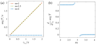
Figure 1: Manybody topological invariant for $CR$-symmetric $(3+1)$d boundary unitary (Sec. VI.3). The invariant was computed via (153) for the ground state of the lattice Hamiltonian (A) in the doubled Hilbert space. The topological phase of the lattice Hamiltonian (i.e., when $2<m<3$) is topologically equivalent to $|U\rangle\!\rangle$.

Figure 1(a) shows how the argument of the following quantity

$${\cal T}(\gamma_{z})=\langle{\it GS}(\Phi_{xy}=2\pi,\gamma_{z})|{\it CR}|{\it GS}(\Phi_{xy}=2\pi,-\gamma_{z})\rangle,$$ (153)

varies as a function of $\gamma_{z}$. We plotted two values for the mass term in the topological phase and one in the trivial phase. It is evident that in the former case $\arg{\cal T}=\gamma_{z}$ while in the latter $\arg{\cal T}=0$. We further check that the linear behavior $\arg{\cal T}=\gamma_{z}$ is valid within the topological phase (away from the transition point $m=3$ where finite-size effects dominate) in Fig. 1(b).

Given the topological equivalence between the topological phase of $\mathbb{H}_{\text{latt}}$ and the ground state of $\mathbb{H}$, we deduce Eq. (133).

References

- (1) T. Oka and H. Aoki, “Photovoltaic Hall effect in graphene,” Phys. Rev. B, vol. 79, p. 081406, Feb. 2009.
- (2) T. Kitagawa, E. Berg, M. Rudner, and E. Demler, “Topological characterization of periodically driven quantum systems,” Phys. Rev. B, vol. 82, p. 235114, Dec. 2010.
- (3) N. H. Lindner, G. Refael, and V. Galitski, “Floquet topological insulator in semiconductor quantum wells,” Nature Physics, vol. 7, pp. 490–495, June 2011.
- (4) L. Jiang, T. Kitagawa, J. Alicea, A. R. Akhmerov, D. Pekker, G. Refael, J. I. Cirac, E. Demler, M. D. Lukin, and P. Zoller, “Majorana Fermions in Equilibrium and in Driven Cold-Atom Quantum Wires,” Physical Review Letters, vol. 106, p. 220402, June 2011.
- (5) T. Oka and S. Kitamura, “Floquet Engineering of Quantum Materials,” ArXiv e-prints, Apr. 2018.
- (6) M. S. Rudner and N. H. Lindner, “Band structure engineering and non-equilibrium dynamics in Floquet topological insulators,” Nature Reviews Physics, vol. 2, pp. 229–244, May 2020.
- (7) F. Harper, R. Roy, M. S. Rudner, and S. L. Sondhi, “Topology and Broken Symmetry in Floquet Systems,” arXiv e-prints, p. arXiv:1905.01317, May 2019.
- (8) Y.-G. Peng, C.-Z. Qin, D.-G. Zhao, Y.-X. Shen, X.-Y. Xu, M. Bao, H. Jia, and X.-F. Zhu, “Experimental demonstration of anomalous floquet topological insulator for sound,” Nature communications, vol. 7, no. 1, pp. 1–8, 2016.
- (9) M. D. Reichl and E. J. Mueller, “Floquet edge states with ultracold atoms,” Physical Review A, vol. 89, no. 6, p. 063628, 2014.
- (10) Q. Cheng, Y. Pan, H. Wang, C. Zhang, D. Yu, A. Gover, H. Zhang, T. Li, L. Zhou, and S. Zhu, “Observation of anomalous modes in photonic floquet engineering,” Physical Review Letters, vol. 122, no. 17, p. 173901, 2019.
- (11) A. Eckardt, “Colloquium: Atomic quantum gases in periodically driven optical lattices,” Reviews of Modern Physics, vol. 89, p. 011004, Jan. 2017.
- (12) M. S. Rudner, N. H. Lindner, E. Berg, and M. Levin, “Anomalous edge states and the bulk-edge correspondence for periodically driven two-dimensional systems,” Physical Review X, vol. 3, no. 3, p. 031005, 2013.
- (13) H. C. Po, L. Fidkowski, T. Morimoto, A. C. Potter, and A. Vishwanath, “Chiral floquet phases of many-body localized bosons,” Physical Review X, vol. 6, no. 4, p. 041070, 2016.
- (14) L. Fidkowski, H. C. Po, A. C. Potter, and A. Vishwanath, “Interacting invariants for Floquet phases of fermions in two dimensions,” ArXiv e-prints, Mar. 2017.
- (15) F. Harper and R. Roy, “Floquet Topological Order in Interacting Systems of Bosons and Fermions,” Physical Review Letters, vol. 118, p. 115301, Mar. 2017.
- (16) C. W. von Keyserlingk and S. L. Sondhi, “Phase structure of one-dimensional interacting Floquet systems. I. Abelian symmetry-protected topological phases,” Phys. Rev. B, vol. 93, p. 245145, June 2016.
- (17) D. V. Else and C. Nayak, “Classification of topological phases in periodically driven interacting systems,” Phys. Rev. B, vol. 93, p. 201103, May 2016.
- (18) A. C. Potter, T. Morimoto, and A. Vishwanath, “Classification of Interacting Topological Floquet Phases in One Dimension,” Physical Review X, vol. 6, p. 041001, Oct. 2016.
- (19) R. Roy and F. Harper, “Floquet topological phases with symmetry in all dimensions,” Phys. Rev. B, vol. 95, p. 195128, May 2017.
- (20) R. Roy and F. Harper, “Periodic table for Floquet topological insulators,” Phys. Rev. B, vol. 96, p. 155118, Oct. 2017.
- (21) S. Yao, Z. Yan, and Z. Wang, “Topological invariants of Floquet systems: General formulation, special properties, and Floquet topological defects,” Phys. Rev. B, vol. 96, p. 195303, Nov. 2017.
- (22) X.-L. Qi, T. L. Hughes, and S.-C. Zhang, “Topological field theory of time-reversal invariant insulators,” Phys. Rev. B, vol. 78, p. 195424, Nov. 2008.
- (23) X. Chen, Z.-C. Gu, Z.-X. Liu, and X.-G. Wen, “Symmetry protected topological orders and the group cohomology of their symmetry group,” Phys. Rev. B, vol. 87, p. 155114, Apr. 2013.
- (24) A. Kapustin, “Symmetry Protected Topological Phases, Anomalies, and Cobordisms: Beyond Group Cohomology,” arXiv e-prints, p. arXiv:1403.1467, Mar. 2014.
- (25) A. Kapustin, “Bosonic Topological Insulators and Paramagnets: a view from cobordisms,” arXiv e-prints, p. arXiv:1404.6659, Apr. 2014.
- (26) A. Kapustin, R. Thorngren, A. Turzillo, and Z. Wang, “Fermionic symmetry protected topological phases and cobordisms,” Journal of High Energy Physics, vol. 2015, p. 52, Dec. 2015.
- (27) M. Levin and Z.-C. Gu, “Braiding statistics approach to symmetry-protected topological phases,” Phys. Rev. B, vol. 86, p. 115109, Sept. 2012.
- (28) S. Ryu and S.-C. Zhang, “Interacting topological phases and modular invariance,” Phys. Rev. B, vol. 85, p. 245132, June 2012.
- (29) O. M. Sule, X. Chen, and S. Ryu, “Symmetry-protected topological phases and orbifolds: Generalized laughlin’s argument,” Phys. Rev. B, vol. 88, p. 075125, Aug 2013.
- (30) H. Shapourian, K. Shiozaki, and S. Ryu, “Partial time-reversal transformation and entanglement negativity in fermionic systems,” Phys. Rev. B, vol. 95, p. 165101, Apr. 2017.
- (31) C.-K. Chiu, J. C. Y. Teo, A. P. Schnyder, and S. Ryu, “Classification of topological quantum matter with symmetries,” Reviews of Modern Physics, vol. 88, p. 035005, July 2016.
- (32) J. I. Cirac, D. Perez-Garcia, N. Schuch, and F. Verstraete, “Matrix product unitaries: structure, symmetries, and topological invariants,” Journal of Statistical Mechanics: Theory and Experiment, vol. 8, p. 083105, Aug. 2017.
- (33) M. B. Şahinoǧlu, S. K. Shukla, F. Bi, and X. Chen, “Matrix product representation of locality preserving unitaries,” Phys. Rev. B, vol. 98, p. 245122, Dec. 2018.
- (34) J. Haah, L. Fidkowski, and M. B. Hastings, “Nontrivial Quantum Cellular Automata in Higher Dimensions,” arXiv e-prints, p. arXiv:1812.01625, Dec. 2018.
- (35) Z. Gong, C. Sünderhauf, N. Schuch, and J. I. Cirac, “Classification of Matrix-Product Unitaries with Symmetries,” arXiv e-prints, p. arXiv:1812.09183, Dec. 2018.
- (36) M. Freedman and M. B. Hastings, “Classification of Quantum Cellular Automata,” arXiv e-prints, p. arXiv:1902.10285, Feb. 2019.
- (37) L. Piroli and J. I. Cirac, “Quantum Cellular Automata, Tensor Networks, and Area Laws,” arXiv e-prints, p. arXiv:2007.15371, July 2020.
- (38) L. Piroli, A. Turzillo, S. K. Shukla, and J. I. Cirac, “Fermionic quantum cellular automata and generalized matrix product unitaries,” arXiv e-prints, p. arXiv:2007.11905, July 2020.
- (39) L. M. Sieberer, A. Chiocchetta, A. Gambassi, U. C. Täuber, and S. Diehl, “Thermodynamic equilibrium as a symmetry of the Schwinger-Keldysh action,” Phys. Rev. B, vol. 92, p. 134307, Oct 2015.
- (40) P. Glorioso and H. Liu, “Lectures on non-equilibrium effective field theories and fluctuating hydrodynamics,” arXiv e-prints, p. arXiv:1805.09331, May 2018.
- (41) A. Altland, M. Fleischhauer, and S. Diehl, “Symmetry classes of open fermionic quantum matter,” arXiv e-prints, p. arXiv:2007.10448, July 2020.
- (42) P. Titum, E. Berg, M. S. Rudner, G. Refael, and N. H. Lindner, “Anomalous Floquet-Anderson Insulator as a Nonadiabatic Quantized Charge Pump,” Physical Review X, vol. 6, p. 021013, Apr. 2016.
- (43) F. Nathan, M. S. Rudner, N. H. Lindner, E. Berg, and G. Refael, “Quantized Magnetization Density in Periodically Driven Systems,” Physical Review Letters, vol. 119, p. 186801, Nov. 2017.
- (44) F. Nathan, D. A. Abanin, N. H. Lindner, E. Berg, and M. S. Rudner, “Hierarchy of many-body invariants and quantized magnetization in anomalous Floquet insulators,” arXiv e-prints, p. arXiv:1907.12228, Jul 2019.
- (45) C. Zhang and M. Levin, “Classification of interacting Floquet phases with symmetry in two dimensions,” arXiv e-prints, p. arXiv:2010.02253, Oct. 2020.
- (46) P. Glorioso, A. Gromov, and S. Ryu, “Effective response theory for Floquet topological systems,” arXiv e-prints, p. arXiv:1908.03217, Aug 2019.
- (47) S. Ryu, A. P. Schnyder, A. Furusaki, and A. W. W. Ludwig, “Topological insulators and superconductors: tenfold way and dimensional hierarchy,” New Journal of Physics, vol. 12, p. 065010, June 2010.
- (48) H. Umezawa, Advanced field theory: Micro, macro, and thermal physics. 1993.
- (49) I. Ojima, “Gauge Fields at Finite Temperatures: Thermo Field Dynamics, KMS Condition and their Extension to Gauge Theories,” Annals Phys., vol. 137, p. 1, 1981.
- (50) C.-T. Hsieh, O. M. Sule, G. Y. Cho, S. Ryu, and R. G. Leigh, “Symmetry-protected topological phases, generalized Laughlin argument, and orientifolds,” Phys. Rev. B, vol. 90, p. 165134, Oct. 2014.
- (51) R. Dijkgraaf and E. Witten, “Topological gauge theories and group cohomology,” Communications in Mathematical Physics, vol. 129, pp. 393–429, Apr. 1990.
- (52) K. Shiozaki and S. Ryu, “Matrix product states and equivariant topological field theories for bosonic symmetry-protected topological phases in (1+1) dimensions,” Journal of High Energy Physics, vol. 2017, p. 100, Apr. 2017.
- (53) D. S. Freed and M. J. Hopkins, “Reflection positivity and invertible topological phases,” arXiv:1604.06527, Apr 2016.
- (54) M. Crossley, P. Glorioso, and H. Liu, “Effective field theory of dissipative fluids,” JHEP, vol. 09, p. 095, 2017.
- (55) J. Haegeman, D. Pérez-García, I. Cirac, and N. Schuch, “Order Parameter for Symmetry-Protected Phases in One Dimension,” Phys. Rev. Lett. , vol. 109, p. 050402, Aug. 2012.
- (56) X. Chen, Z.-C. Gu, and X.-G. Wen, “Classification of gapped symmetric phases in one-dimensional spin systems,” Phys. Rev. B, vol. 83, p. 035107, Jan. 2011.
- (57) N. Schuch, D. Pérez-García, and I. Cirac, “Classifying quantum phases using matrix product states and projected entangled pair states,” Phys. Rev. B, vol. 84, p. 165139, Oct. 2011.
- (58) F. Pollmann, E. Berg, A. M. Turner, and M. Oshikawa, “Symmetry protection of topological phases in one-dimensional quantum spin systems,” Phys. Rev. B, vol. 85, p. 075125, Feb. 2012.
- (59) S. Higashikawa, M. Nakagawa, and M. Ueda, “Floquet Chiral Magnetic Effect,” Phys. Rev. Lett. , vol. 123, p. 066403, Aug. 2019.
- (60) X. Chen, Z.-X. Liu, and X.-G. Wen, “Two-dimensional symmetry-protected topological orders and their protected gapless edge excitations,” Phys. Rev. B, vol. 84, p. 235141, Dec. 2011.
- (61) N. Sannomiya and H. Katsura, “Supersymmetry Breaking and Nambu-Goldstone Fermions in Interacting Majorana Chains,” arXiv e-prints, p. arXiv:1712.01148, Dec. 2017.
- (62) T. H. Hsieh, G. B. Halász, and T. Grover, “All Majorana Models with Translation Symmetry are Supersymmetric,” Phys. Rev. Lett. , vol. 117, p. 166802, Oct. 2016.
- (63) L. Fidkowski and A. Kitaev, “Effects of interactions on the topological classification of free fermion systems,” Phys. Rev. B, vol. 81, p. 134509, Apr. 2010.
- (64) L. Fidkowski and A. Kitaev, “Topological phases of fermions in one dimension,” Phys. Rev. B, vol. 83, p. 075103, Feb. 2011.
- (65) A. Kapustin, R. Thorngren, A. Turzillo, and Z. Wang, “Fermionic symmetry protected topological phases and cobordisms,” Journal of High Energy Physics, vol. 2015, p. 1–21, Dec 2015.
- (66) K. Shiozaki, H. Shapourian, and S. Ryu, “Many-body topological invariants in fermionic symmetry-protected topological phases: Cases of point group symmetries,” Physical Review B, vol. 95, p. 205139, May 2017.
- (67) G. Y. Cho, C.-T. Hsieh, T. Morimoto, and S. Ryu, “Topological phases protected by reflection symmetry and cross-cap states,” Phys. Rev. B, vol. 91, p. 195142, May 2015.
- (68) G. Y. Cho, K. Shiozaki, S. Ryu, and A. W. W. Ludwig, “Relationship between symmetry protected topological phases and boundary conformal field theories via the entanglement spectrum,” Journal of Physics A Mathematical General, vol. 50, p. 304002, July 2017.
- (69) S. Ryu and S.-C. Zhang, “Interacting topological phases and modular invariance,” Physical Review B, vol. 85, Jun 2012.
- (70) X.-L. Qi, “A new class of (2 + 1)-dimensional topological superconductors with topological classification,” New Journal of Physics, vol. 15, p. 065002, Jun 2013.
- (71) H. Shapourian and S. Ryu, “Entanglement negativity of fermions: Monotonicity, separability criterion, and classification of few-mode states,” Phys. Rev. A, vol. 99, p. 022310, Feb. 2019.
- (72) K. Shiozaki, H. Shapourian, K. Gomi, and S. Ryu, “Many-body topological invariants for fermionic short-range entangled topological phases protected by antiunitary symmetries,” Phys. Rev. B, vol. 98, p. 035151, July 2018.
- (73) P. Glorioso and H. Liu, “The second law of thermodynamics from symmetry and unitarity,” 2016.
- (74) X.-Q. Sun, M. Xiao, T. Bzdušek, S.-C. Zhang, and S. Fan, “Three-Dimensional Chiral Lattice Fermion in Floquet Systems,” Phys. Rev. Lett. , vol. 121, p. 196401, Nov. 2018.
- (75) T. Iadecola and T. H. Hsieh, “Floquet Supersymmetry,” Phys. Rev. Lett. , vol. 120, p. 210603, May 2018.
- (76) M. Schecter and T. Iadecola, “Many-body spectral reflection symmetry and protected infinite-temperature degeneracy,” Phys. Rev. B, vol. 98, p. 035139, July 2018.