UMTG–308

Factorization identities and algebraic Bethe ansatz
for $D^{(2)}_{2}$ models
Rafael I. Nepomechie and Ana L. Retore

We express $D^{(2)}_{2}$ transfer matrices as products of $A^{(1)}_{1}$ transfer matrices, for both closed and open spin chains. We use these relations, which we call factorization identities, to solve the models by algebraic Bethe ansatz. We also formulate and solve a new integrable XXZ-like open spin chain with an even number of sites that depends on a continuous parameter, which we interpret as the rapidity of the boundary.

1 Introduction

The antiferromagnetic Potts model and the staggered six-vertex model [1, 2, 3, 4, 5, 6, 7, 8, 9, 10, 11] have recently been shown [12] to be related to the $D^{(2)}_{2}$ R-matrix [13, 14, 15]. Even more recently, an open $D^{(2)}_{2}$ spin chain with a particular integrable boundary condition has been shown [16] to have as its continuum limit a non-compact boundary conformal field theory, which possesses a continuous spectrum of conformal dimensions; it is closely related to the $SL(2,\mathbb{R})/U(1)$ Euclidean black hole [17, 18, 19, 20, 21], see also [22, 23, 24].

Here we express the $D^{(2)}_{2}$ transfer matrices for the open spin chains considered in [12] and [16] as products of $A^{(1)}_{1}$ transfer matrices. We then use these relations, which we call factorization identities, to solve the models by algebraic Bethe ansatz. In particular, we construct the models’ Bethe states, which had not been known, that would be needed to compute scalar products and correlation functions. Moreover, we prove previously-proposed expressions for the models’ eigenvalues and Bethe equations [16, 25, 26, 27, 28]. The interesting degeneracies exhibited by these models are also explained.

In the course of this work, we also formulate and solve a new integrable XXZ-like open spin chain, which depends on a continuous parameter. We interpret this parameter as the rapidity of the boundary. We conjecture that this model, like the one in [16], has a non-compact continuum limit.

This paper is structured as follows. In Sec. 2, we give an exact formulation (2.11)-(2.12) of the factorization [12] of the $D^{(2)}_{2}$ R-matrix in terms of $A^{(1)}_{1}$ R-matrices. Sec. 3 is devoted to the closed $D^{(2)}_{2}$ spin chain. We use the factorization of the R-matrix to derive the factorization identity (3.9)-(3.10), which expresses the $D^{(2)}_{2}$ transfer matrix as a product of $A^{(1)}_{1}$ transfer matrices. We then use this identity to solve the model by means of algebraic Bethe ansatz. Since these computations are straightforward, they may serve as a warm-up exercise for the parallel – but technically more complicated – computations that follow.

The heart of this paper is Sec. 4, where we consider open $D^{(2)}_{2}$ chains with two different sets of integrable boundary conditions, corresponding to the two possible values (namely, 0 and 1) of a certain parameter $\varepsilon$. We consider first the case $\varepsilon=1$, which was studied in [16]. The factorization identity (4.10)-(4.11), whose derivation is presented in Appendix A, involves a novel $A^{(1)}_{1}$ transfer matrix (4.12). It is a special case of the more general transfer matrix (4.15), which depends on an arbitrary parameter $u_{0}$ that (as remarked above) we interpret as the rapidity of the boundary. We solve the general model by algebraic Bethe ansatz, from which we then extract the solution for the case $\varepsilon=1$. We treat the case $\varepsilon=0$, which was studied in [12], in a similar way. Its factorization identity (4.59)-(4.60), whose derivation is also presented in Appendix A, involves a conventional $A^{(1)}_{1}$ transfer matrix (4.61), corresponding to $u_{0}=0$. In Sec. 5, we point out a special case of the model (4.15) with a local Hamiltonian for general values of $u_{0}$. We conclude with a brief discussion of our results in Sec. 6.

2 Product-form R-matrices

We begin this section by reviewing in Sec. 2.1 a well-known general recipe for constructing an R-matrix by forming suitable tensor products of multiple copies of a more elementary R-matrix. We actually need a (perhaps less familiar) generalization of this construction, namely (2.6). Indeed, in Sec. 2.2, we see that the recent factorization [12] of the $D^{(2)}_{2}$ R-matrix in terms of $A^{(1)}_{1}$ R-matrices is precisely of this type, up to a similarity transformation. The result (2.11)-(2.12) is the basis for all the factorization identities that we will derive in this paper, which express $D^{(2)}_{2}$ transfer matrices as products of $A^{(1)}_{1}$ transfer matrices.

2.1 Generalities

Consider a solution $R(u)$ of the Yang-Baxter equation (YBE)

$$R_{12}(u-v)\,R_{13}(u)\,R_{23}(v)=R_{23}(v)\,R_{13}(u)\,R_{12}(u-v)\,.$$ (2.1)

As usual, $R(u)$ is a $d^{2}\times d^{2}$ matrix that maps ${\cal V}\otimes{\cal V}\mapsto{\cal V}\otimes{\cal V}$, where ${\cal V}$ is a $d$-dimensional vector space. In (2.1), $R_{12}=R\otimes\mathbb{I}\,,R_{23}=\mathbb{I}\otimes R\,,R_{13}={\cal P}_{23}R_{12}{\cal P}_{23}$, where here $\mathbb{I}$ is the identity matrix on ${\cal V}$ (below, by abuse of notation, $\mathbb{I}$ may denote the identity matrix on more than one copy of ${\cal V}$, depending on the context), and ${\cal P}$ is the permutation matrix on ${\cal V}\otimes{\cal V}$

$${\cal P}=\sum_{a,b=1}^{d}e_{ab}\otimes e_{ba}\,,$$ (2.2)

where $e_{ab}$ are the $d\times d$ elementary matrices with elements $(e_{ab})_{ij}=\delta_{a,i}\delta_{b,j}$. As is well known, the R-matrix can be usefully represented graphically by one pair of lines that cross, as shown in Fig. 2; hence the YBE (2.1) is represented using three lines, as shown in Fig. 2.

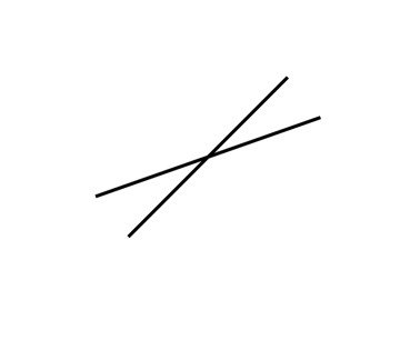
Figure 1: $R(u)$

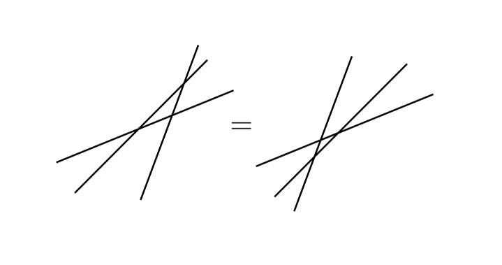
Figure 2: YBE for $R(u)$

We assume that the R-matrix is regular

$$R(0)\propto{\cal P}\,,$$ (2.3)

and unitary

$$R_{12}(u)\,R_{21}(-u)\propto\mathbb{I}\,,$$ (2.4)

where $R_{21}={\cal P}_{12}\,R_{12}\,{\cal P}_{12}$. We use the symbol $\propto$ to denote equality up to a scalar factor. The latter can be represented graphically as in Fig. 3.

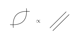
Figure 3: Unitarity

Another solution $\mathbb{R}(u)$ of the YBE, which maps $({\cal V}\otimes{\cal V})\otimes({\cal V}\otimes{\cal V})\mapsto({\cal V}\otimes{\cal V})\otimes({\cal V}\otimes{\cal V})$ is given by the following product of four R-matrices

$$\mathbb{R}_{12,34}(u)=R_{14}(u)\,R_{13}(u)\,R_{24}(u)\,R_{23}(u)\,,$$ (2.5)

which is a $d^{4}\times d^{4}$ matrix. This R-matrix can be represented graphically by two pairs of lines that cross, as shown in Fig. 5. The corresponding YBE for $\mathbb{R}$, represented in Fig. 5, follows from the YBE for $R$ shown in Fig. 2. A review of models constructed with R-matrices of this type can be found in [29].

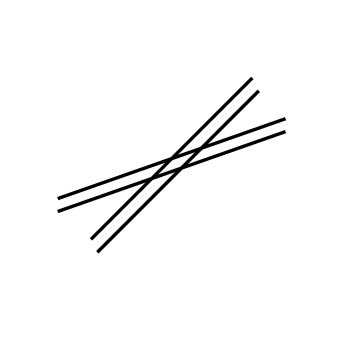
Figure 4: $\mathbb{R}(u)$ in Eq. (2.5)

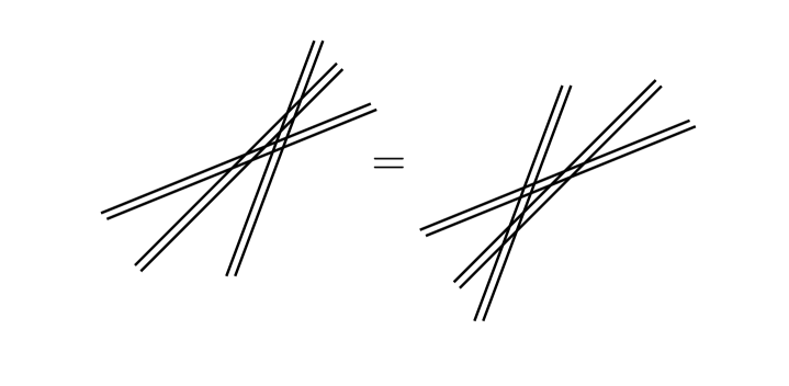
Figure 5: YBE for $\mathbb{R}(u)$ in Eq. (2.5)

We will need a generalization of the construction (2.5), namely,

$$\mathbb{R}_{12,34}(u)=R_{43}(-\theta)R_{13}(u)\,R_{14}(u+\theta)\,R_{23}(u-\theta)\,R_{24}(u)\,R_{34}(\theta)\,,$$ (2.6)

where $\theta$ is an arbitrary constant, see Fig. 7. Indeed, using the regularity property (2.3), the construction (2.6) reduces to (2.5) for $\theta=0$. The proof that (2.6) satisfies the YBE, which requires unitarity (2.4) as well as the YBE (2.1), can also be performed graphically (see Fig. 7), or by a straightforward but long explicit computation.

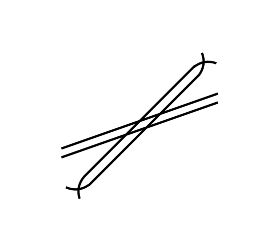
Figure 6: $\mathbb{R}(u)$ in Eq. (2.6)

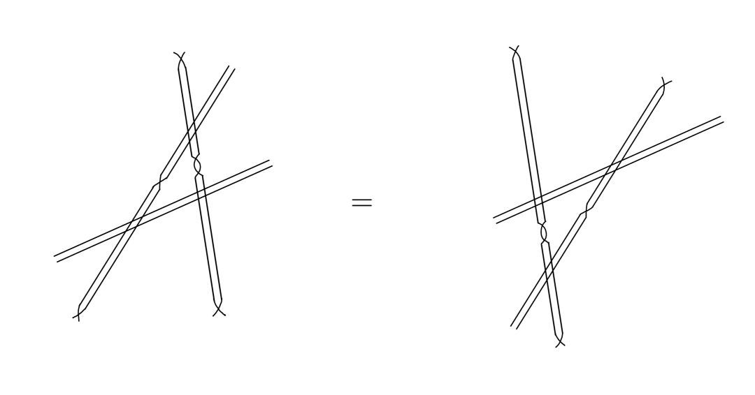
Figure 7: YBE for $\mathbb{R}(u)$ in Eq. (2.6)

2.2 The $D^{(2)}_{2}$ R-matrix

The $D^{(2)}_{2}$ R-matrix, following a hint from [30, 31], has recently been shown [12] to be of product form, up to a similarity transformation. Indeed, let us write the $D^{(2)}_{2}$ R-matrix from [14] as in Appendix A of [27], with spectral parameter $u$ and anisotropy parameter $\eta$, and denote it by $\tilde{\mathbb{R}}(u)$. Then

$$\tilde{\mathbb{R}}_{12,34}(u)\propto B_{12}\,B_{34}\,\mathbb{R}_{12,34}(u)\,B_{12}\,B_{34}\,,$$ (2.7)

where $\mathbb{R}(u)$ is given by (2.6), with $R(u)$ given by the $A^{(1)}_{1}$ (XXZ) R-matrix

$$R(u)=\left(\begin{array}[]{cccc}\sinh(-\tfrac{u}{2}+\eta)&0&0&0\\ 0&\sinh(\tfrac{u}{2})&e^{-\frac{u}{2}}\sinh(\eta)&0\\ 0&e^{\frac{u}{2}}\sinh(\eta)&\sinh(\tfrac{u}{2})&0\\ 0&0&0&\sinh(-\tfrac{u}{2}+\eta)\end{array}\right)\,,$$ (2.8)

and $\theta=i\pi$. Moreover, the similarity transformation is given by

$$B=\left(\begin{array}[]{cccc}1&0&0&0\\ 0&\frac{\cosh\left(\tfrac{\eta}{2}\right)}{\sqrt{\cosh\eta}}&-\frac{\sinh\left(\tfrac{\eta}{2}\right)}{\sqrt{\cosh\eta}}&0\\[5.69046pt] 0&-\frac{\sinh\left(\tfrac{\eta}{2}\right)}{\sqrt{\cosh\eta}}&-\frac{\cosh\left(\tfrac{\eta}{2}\right)}{\sqrt{\cosh\eta}}&0\\[5.69046pt] 0&0&0&1\end{array}\right),\,\qquad B^{2}=\mathbb{I}\,.$$ (2.9)

Following [5, 7], we define the matrix $C$ by

$$C=\frac{i}{\cosh\eta}{\cal P}R(i\pi)\,,\qquad C^{2}=\mathbb{I}\,.$$ (2.10)

Using this notation, the result (2.6)-(2.7) for the $D^{(2)}_{2}$ R-matrix takes the final form

$$\tilde{\mathbb{R}}_{12,34}(u)=B_{12}\,B_{34}\,\mathbb{R}_{12,34}(u)\,B_{12}\,B_{34}\,,$$ (2.11)

where $\mathbb{R}(u)$ has been redefined (by a simple rescaling) as

$$\mathbb{R}_{12,34}(u)=2^{4}\,C_{34}\,R_{14}(u)\,R_{13}(u+i\pi)\,R_{24}(u-i\pi)\,R_{23}(u)\,C_{34}\,.$$ (2.12)

Note that we use a tilde to denote similarity-transformed quantities. Eqs. (2.11)-(2.12) are an exact formulation, in our notation, of the factorization discovered in [12]. In the isotropic limit $\eta\rightarrow 0$, this result reduces to the fact (see e.g. [32]) that the $D_{2}$ (i.e. $SO(4)$) R-matrix factorizes into a product of two $A_{1}$ (i.e. $SU(2)$) R-matrices, up to a similarity transformation.

For future reference, we note here some useful properties of the R-matrix (2.8) in addition to (2.1)-(2.4): quasi-periodicity

$$R(u+2i\pi)=-R(u)\,,$$ (2.13)

PT-symmetry

$$R_{12}^{t_{1}t_{2}}(u)=R_{21}(u)$$ (2.14)

(where $t_{i}$ denotes transposition in the $i^{th}$ vector space), and crossing-unitarity

$$R_{12}^{t_{1}}(u)\,M_{1}\,R_{12}^{t_{2}}(-u+4\eta)\,M^{-1}_{1}=-\sinh(\tfrac{u}{2})\,\sinh(\tfrac{u}{2}-2\eta)\,\mathbb{I}\,,\qquad M=\mathop{\rm diag}\nolimits\left(e^{\eta}\,,e^{-\eta}\right)\,.$$ (2.15)

3 The closed $D^{(2)}_{2}$ spin chain

We begin with the simplest case, namely, the closed periodic $D^{(2)}_{2}$ spin chain. In Sec. 3.1, we use the factorization of the R-matrix (2.11)-(2.12) to derive the factorization identity (3.9)-(3.10) that expresses the $D^{(2)}_{2}$ transfer matrix as a product of $A^{(1)}_{1}$ transfer matrices. In Sec. 3.2, we use this identity to solve the model by means of algebraic Bethe ansatz.

3.1 Factorization identity

The monodromy matrix for a chain of length $N$ is defined by

$$\tilde{\mathbb{T}}_{0}(u)=\tilde{\mathbb{R}}_{0N}(u)\,\ldots\tilde{\mathbb{R}}_{01}(u)\,,$$ (3.1)

where $\tilde{\mathbb{R}}(u)$ is the $D^{(2)}_{2}$ R-matrix. In order to exploit the factorization (2.11)-(2.12), it is convenient to replace each index $j$ in (3.1) (which corresponds to a 4-dimensional vector space) by a pair of indices $\bar{j}\,,\bar{\bar{j}}$ (each of which corresponds to a 2-dimensional vector space). In this way, the monodromy matrix takes the form

$$\tilde{\mathbb{T}}_{0}(u)=\tilde{\mathbb{T}}_{\bar{0}\bar{\bar{0}}}(u)=\tilde{\mathbb{R}}_{\bar{0}\bar{\bar{0}},\bar{N}\bar{\bar{N}}}(u)\,\ldots\tilde{\mathbb{R}}_{\bar{0}\bar{\bar{0}},\bar{1}\bar{\bar{1}}}(u)\,.$$ (3.2)

The relation (2.11) implies

$$\tilde{\mathbb{T}}_{\bar{0}\bar{\bar{0}}}(u)=B_{\bar{0}\bar{\bar{0}}}\,\mathbb{B}\,\mathbb{T}_{\bar{0}\bar{\bar{0}}}(u)\,\mathbb{B}\,B_{\bar{0}\bar{\bar{0}}}\,,$$ (3.3)

where $\mathbb{T}_{\bar{0}\bar{\bar{0}}}(u)$ is defined in terms of $\mathbb{R}$’s as in (3.2) except without tildes, and $\mathbb{B}$ is the quantum-space operator

$$\mathbb{B}=B_{\bar{1}\bar{\bar{1}}}\,\ldots B_{\bar{N}\bar{\bar{N}}}\,.$$ (3.4)

Using (2.12), we obtain

$$\mathbb{T}_{\bar{0}\bar{\bar{0}}}(u)=2^{4N}\,\mathbb{C}\,T_{\bar{0}}(u)\,T_{\bar{\bar{0}}}(u-i\pi)\,\mathbb{C}\,,$$ (3.5)

where $T_{\bar{0}}(u)$ is defined by

$$T_{\bar{0}}(u)=R_{\bar{0}\bar{\bar{N}}}(u)\,R_{\bar{0}\bar{N}}(u+i\pi)\ldots R_{\bar{0}\bar{\bar{1}}}(u)\,R_{\bar{0}\bar{1}}(u+i\pi)\,,$$ (3.6)

and $\mathbb{C}$ is the quantum-space operator

$$\mathbb{C}=C_{\bar{1}\bar{\bar{1}}}\,\ldots C_{\bar{N}\bar{\bar{N}}}\,.$$ (3.7)

Note that $T_{\bar{0}}(u)$ is a monodromy matrix on $2N$ sites, with $i\pi$ shifts on alternating sites; $T_{\bar{\bar{0}}}(u)$ is given by the same expression (3.6), except with $\bar{0}$ replaced by $\bar{\bar{0}}$. Note also the periodicity $T_{\bar{0}}(u+2i\pi)=T_{\bar{0}}(u)$ as a consequence of (2.13).

The transfer matrix for the closed periodic spin chain is obtained by tracing the monodromy matrix over the auxiliary space

$$\tilde{\mathbbm{t}}(u)=\mathop{\rm tr}\nolimits_{0}\tilde{\mathbb{T}}_{0}(u)=\mathop{\rm tr}\nolimits_{\bar{0}\bar{\bar{0}}}\tilde{\mathbb{T}}_{\bar{0}\bar{\bar{0}}}(u)\,.$$ (3.8)

Eq. (3.3) implies

$$\tilde{\mathbbm{t}}(u)=\mathbb{B}\,\mathbbm{t}(u)\,\mathbb{B}\,,$$ (3.9)

where $\mathbbm{t}(u)$ is defined in terms of $\mathbb{T}(u)$ as in (3.8) except without tildes. Using (3.5), we immediately obtain the result

$$\mathbbm{t}(u)=2^{4N}\,\mathbb{C}\,t(u)\,t(u-i\pi)\,\mathbb{C}\,,$$ (3.10)

where $t(u)$ is an $A^{(1)}_{1}$ closed-chain transfer matrix defined by

$$t(u)=\mathop{\rm tr}\nolimits_{\bar{0}}T_{\bar{0}}(u)\,.$$ (3.11)

The result (3.9)-(3.10), which we call a factorization identity, shows that, up to similarity transformations, the $D^{(2)}_{2}$ closed-chain transfer matrix is given by a product of $A^{(1)}_{1}$ closed-chain transfer matrices with twice as many sites.

3.2 Algebraic Bethe ansatz

We now proceed to determine the eigenvectors and eigenvalues of the $D^{(2)}_{2}$ closed-chain transfer matrix $\tilde{\mathbbm{t}}(u)$ using the factorization identity (3.9)-(3.10).

To this end, we recall (see e.g. [33]) that the $A^{(1)}_{1}$ transfer matrix can be diagonalized by algebraic Bethe ansatz. Indeed, consider the general inhomogeneous monodromy matrix with length $L$

$$T_{0}(u;\{\theta_{l}\})=R_{0L}(u-\theta_{L})\,\ldots R_{01}(u-\theta_{1})=\left(\begin{array}[]{cc}*&{\cal B}(u;\{\theta_{l}\})\\ &*\end{array}\right)\,,$$ (3.12)

where $R(u)$ is given by (2.8), and $\{\theta_{l}\}$ are arbitrary inhomogeneities. (The indices here correspond to 2-dimensional vector spaces, i.e., the same as $\bar{j}$ and $\bar{\bar{j}}$ in (3.6).) We denote the corresponding closed-chain transfer matrix by

$$t(u;\{\theta_{l}\})=\mathop{\rm tr}\nolimits_{0}T_{0}(u;\{\theta_{l}\})\,.$$ (3.13)

The operator ${\cal B}(u;\{\theta_{l}\})$ in (3.12) serves as a creation operator on the reference state

$$|0\rangle={1\choose 0}^{\otimes L}\,.$$ (3.14)

The Bethe states defined by

$$|v_{1}\cdots v_{m}\rangle=\prod_{k=1}^{m}{\cal B}(v_{k};\{\theta_{l}\})\,|0\rangle$$ (3.15)

can be shown to obey the following off-shell equation

$$t(u;\{\theta_{l}\})\,|v_{1}\cdots v_{m}\rangle=\chi(u;\{\theta_{l}\})\,|v_{1}\cdots v_{m}\rangle+\sum_{j=1}^{m}\chi_{j}\,|u,v_{1}\cdots\hat{v}_{j}\cdots v_{m}\rangle\,,$$ (3.16)

where the variable with a hat is omitted, and $\chi(u;\{\theta_{l}\})$ is given by

$$\chi(u;\{\theta_{l}\})=(-1)^{m}\left[\frac{q(u+2\eta)}{q(u)}\prod_{l=1}^{L}\sinh(\eta-\tfrac{1}{2}(u-\theta_{l}))+\frac{q(u-2\eta)}{q(u)}\prod_{l=1}^{L}\sinh(\tfrac{1}{2}(u-\theta_{l}))\right]\,,$$ (3.17)

with

$$q(u)=\prod_{k=1}^{m}\sinh(\tfrac{1}{2}(u-v_{k}))\,.$$ (3.18)

Moreover, $\chi_{j}$ is given by

$$\chi_{j} =(-1)^{m+1}\frac{\sinh(\eta)\,e^{\frac{1}{2}(u-v_{j})}}{\sinh(\tfrac{1}{2}(u-v_{j}))}\Bigg{[}\prod_{l=1}^{L}\sinh(\eta-\tfrac{1}{2}(v_{j}-\theta_{l}))\prod_{k=1;k\neq j}^{m}\frac{\sinh(\tfrac{1}{2}(v_{j}-v_{k})+\eta)}{\sinh(\tfrac{1}{2}(v_{j}-v_{k}))}$$

$$\qquad-\prod_{l=1}^{L}\sinh(\tfrac{1}{2}(v_{j}-\theta_{l}))\prod_{k=1;k\neq j}^{m}\frac{\sinh(\tfrac{1}{2}(v_{j}-v_{k})-\eta)}{\sinh(\tfrac{1}{2}(v_{j}-v_{k}))}\Bigg{]}\,.$$ (3.19)

Our original monodromy matrix (3.6) corresponds to setting $L=2N$ in (3.12), and choosing the inhomogeneities as follows

$$\theta_{l}=\begin{cases}-i\pi&\text{for $l=$ odd}\\ 0&\text{for $l=$ even}\end{cases}\,.$$ (3.20)

It follows that the Bethe states (3.15) with these inhomogeneities are eigenstates of our original transfer matrix (3.11), with corresponding eigenvalues given by

$$\chi(u)=(-1)^{m}\left(\tfrac{i}{2}\right)^{N}\left[\sinh^{N}(u-2\eta)\frac{q(u+2\eta)}{q(u)}+\sinh^{N}(u)\frac{q(u-2\eta)}{q(u)}\right]\,,$$ (3.21)

provided that $\{v_{k}\}$ satisfy the Bethe equations

$$\left(\frac{\sinh(v_{j})}{\sinh(v_{j}-2\eta)}\right)^{N}=\prod_{k=1;k\neq j}^{m}\frac{\sinh(\tfrac{1}{2}(v_{j}-v_{k})+\eta)}{\sinh(\tfrac{1}{2}(v_{j}-v_{k})-\eta)}\,.$$ (3.22)

These equations take a symmetric form in terms of $u_{j}\equiv v_{j}-\eta$, namely,

$$\left(\frac{\sinh(u_{j}+\eta)}{\sinh(u_{j}-\eta)}\right)^{N}=\prod_{k=1;k\neq j}^{m}\frac{\sinh(\tfrac{1}{2}(u_{j}-u_{k})+\eta)}{\sinh(\tfrac{1}{2}(u_{j}-u_{k})-\eta)}\,.$$ (3.23)

Setting

$$Q(u)=\prod_{k=1}^{m}\sinh(\tfrac{1}{2}(u-u_{k}))=q(u+\eta)\,,$$ (3.24)

the expression for the eigenvalues (3.21) of the $A^{(1)}_{1}$ closed-chain transfer matrix $t(u)$ (3.11) take the final form

$$\chi(u)=(-1)^{m}\left(\tfrac{i}{2}\right)^{N}\left[\sinh^{N}(u-2\eta)\frac{Q(u+\eta)}{Q(u-\eta)}+\sinh^{N}(u)\frac{Q(u-3\eta)}{Q(u-\eta)}\right]\,.$$ (3.25)

Coming back to the $D^{(2)}_{2}$ closed-chain transfer matrix $\tilde{\mathbbm{t}}(u)$ (3.8), we conclude from the factorization identity (3.9)-(3.10) that its Bethe states are given by

$$\mathbb{B}\,\mathbb{C}\,|v_{1}\cdots v_{m}\rangle\,,$$ (3.26)

where the vectors $|v_{1}\cdots v_{m}\rangle$ are given by (3.15), and $\mathbb{B}$ and $\mathbb{C}$ are given respectively by (3.4) and (3.7), see [30] for an alternative approach. Moreover, the corresponding eigenvalues $\Lambda(u)$ are given by

$$\Lambda(u)=2^{4N}\,\chi(u)\,\chi(u-i\pi)\,,$$ (3.27)

where $\chi(u)$ is given by (3.25), and the associated Bethe equations are given by (3.23). The latter results agree with expressions obtained by Reshetikhin using analytical Bethe ansatz [25].

3.3 $Z_{2}$ symmetry

The transfer matrix $t(u)$ (3.11) has the property

$$\mathbb{C}\,t(u)\,\mathbb{C}=(-1)^{N}\,t(u+i\pi)\,,$$ (3.28)

where $\mathbb{C}$ (3.7) is defined in terms of $C$ (2.10). The proof is short: the fact that the R-matrix satisfies the identity

$$C_{23}\,R_{13}(u)\,R_{12}(u+i\pi)\,C_{23}=R_{13}(u+i\pi)\,R_{12}(u)$$ (3.29)

implies that the monodromy matrix (3.6) satisfies the corresponding identity

$$\mathbb{C}\,T_{\bar{0}}(u)\,\mathbb{C}=(-1)^{N}\,T_{\bar{0}}(u+i\pi)\,.$$ (3.30)

By tracing over the auxiliary space $\bar{0}$, we obtain (3.28).

The property (3.28) implies that the $D^{(2)}_{2}$ transfer matrix $\mathbbm{t}(u)$ (3.10) can also be written in the form

$$\mathbbm{t}(u)=2^{4N}\,t(u+i\pi)\,t(u)\,,$$ (3.31)

and therefore it has the $Z_{2}$ symmetry

$$\mathbb{C}\,\mathbbm{t}(u)\,\mathbb{C}=\mathbbm{t}(u)\,.$$ (3.32)

The $Z_{2}$ symmetry of the staggered six-vertex model was noted already in [7].

3.4 Degeneracies

For real values of $\eta$, each of the eigenvalues of $t(u)$ (3.11) is either a singlet or a doublet (2-fold degenerate). However, as the result of the $Z_{2}$ symmetry, some of the degeneracies of $\mathbbm{t}(u)$ (3.10) become doubled, leading to doublets or quartets.

The key point is that the $Z_{2}$ symmetry shifts the argument of the ${\cal B}$-operator by $i\pi$

$$\mathbb{C}\,{\cal B}(u)\,\mathbb{C}=(-1)^{N}\,{\cal B}(u+i\pi)\,,$$ (3.33)

as follows from (3.12) and (3.30). The Bethe states (3.15) therefore transform as follows

$$\mathbb{C}\,|v_{1}\cdots v_{m}\rangle=(-1)^{N\,m}\,|v_{1}+i\pi\cdots v_{m}+i\pi\rangle\,,$$ (3.34)

since the reference state remains invariant $\mathbb{C}\,|0\rangle=|0\rangle$. In other words, under the $Z_{2}$ symmetry, each of the Bethe roots $v_{k}$ (or, equivalently, $u_{k}$) is shifted by $i\pi$. If $Q(u+i\pi)\neq\pm Q(u)$, then the Bethe states corresponding to $Q(u)$ and $Q(u+i\pi)$ are mapped into each other by the $Z_{2}$ symmetry $\mathbb{C}$. (The argument is the same as for the open chain, which is presented in Sec. 4.2.4.) It follows from (3.32) that the two Bethe states have the same eigenvalue of $\mathbbm{t}(u)$, which means that they are degenerate.

Our goal in the remainder of this paper is to obtain factorization identities analogous to (3.9)-(3.10) for $D^{(2)}_{2}$ open-chain transfer matrices, and use these relations to solve the models.

4 The open $D^{(2)}_{2}$ spin chain

We turn now to the open $D^{(2)}_{2}$ spin chain. We will consider two different sets of integrable boundary conditions, corresponding to the two possible values (namely, 0 and 1) of a certain parameter $\varepsilon$. As before, our strategy will be to use factorization identities to solve the models. After introducing the transfer matrix in Sec. 4.1, we consider the case $\varepsilon=1$ in Sec. 4.2, followed by case $\varepsilon=0$ in Sec. 4.3.

4.1 Transfer matrix

In order to construct an integrable open-chain transfer matrix [34], we need not only an R-matrix, but also a K-matrix, i.e., a solution of the corresponding boundary Yang-Baxter equation [34, 35, 36]. For $D^{(2)}_{n+1}$, such K-matrices have been found in [26, 37]. The K-matrices in [37] depend on two discrete parameters: $p$ (which can take $n+1$ different values, namely, $p=0,1,\ldots,n$) and $\varepsilon$ (which can take two different values, namely, $\varepsilon=0,1$). We consider here $n=1$ (corresponding to $D^{(2)}_{2}$); and, for concreteness, we set $p=0$. (The case $p=1$ is simply related to the case $p=0$ by a $p\leftrightarrow n-p$ duality symmetry [37, 38].) The right K-matrix, which we denote here by $\tilde{\mathbb{K}}^{R}(u)$, is then given by

$$\tilde{\mathbb{K}}^{R}(u)=\left(\begin{array}[]{cccc}g(u)&0&0&0\\ 0&k_{1}(u)&k_{2}(u)&0\\ 0&k_{2}(u)&k_{1}(u)&0\\ 0&0&0&g(u)\end{array}\right)\,,$$ (4.1)

where

$$g(u) =\frac{\cosh(u-\eta+\frac{i\pi}{2}\varepsilon)}{\cosh(u+\eta-\frac{i\pi}{2}\varepsilon)}\,,$$

$$k_{1}(u) =\frac{\cosh(u)\cosh(\eta+\frac{i\pi}{2}\varepsilon)}{\cosh(u+\eta+\frac{i\pi}{2}\varepsilon)}\,,$$

$$k_{2}(u) =-\frac{\sinh(u)\sinh(\eta+\frac{i\pi}{2}\varepsilon)}{\cosh(u+\eta+\frac{i\pi}{2}\varepsilon)}\,,$$ (4.2)

with $\varepsilon=0,1$. For the left K-matrix, we take [37]

$$\tilde{\mathbb{K}}^{L}(u)=\tilde{\mathbb{K}}^{R}(-u+2\eta)\,\mathbb{M}\,,\qquad\mathbb{M}=M\otimes M\,,$$ (4.3)

where $M$ is defined in (2.15), so that the transfer matrix has quantum-group symmetry, see Sec. 4.2.3.

The $D^{(2)}_{2}$ open-chain transfer matrix for a chain with $N$ sites is given by [34]

$$\tilde{\mathbbm{t}}(u)=\mathop{\rm tr}\nolimits_{0}\Big{\{}\tilde{\mathbb{K}}^{L}_{0}(u)\,\tilde{\mathbb{T}}_{0}(u)\,\tilde{\mathbb{K}}^{R}_{0}(u)\,\widehat{\tilde{\mathbb{T}}}_{0}(u)\Big{\}}\,,$$ (4.4)

where $\tilde{\mathbb{T}}_{0}(u)$ is given by (3.1) and (3.2). Similarly, $\widehat{\tilde{\mathbb{T}}}_{0}(u)$ is given by

$$\widehat{\tilde{\mathbb{T}}}_{0}(u)=\tilde{\mathbb{R}}_{10}(u)\,\ldots\tilde{\mathbb{R}}_{N0}(u)\,,$$ (4.5)

or equivalently

$$\widehat{\tilde{\mathbb{T}}}_{\bar{0}\bar{\bar{0}}}(u)=\tilde{\mathbb{R}}_{\bar{1}\bar{\bar{1}},\bar{0}\bar{\bar{0}}}(u)\ldots\tilde{\mathbb{R}}_{\bar{N}\bar{\bar{N}},\bar{0}\bar{\bar{0}}}(u)\,,$$ (4.6)

where we have replaced (as we did for $\tilde{\mathbb{T}}_{0}(u)$ in Sec. 3.1) each index $j$ in (4.5) by a pair of indices $\bar{j}\,,\bar{\bar{j}}$. Eq. (2.11) then implies

$$\widehat{\tilde{\mathbb{T}}}_{\bar{0}\bar{\bar{0}}}(u)=B_{\bar{0}\bar{\bar{0}}}\,\mathbb{B}\,\widehat{\mathbb{T}}_{\bar{0}\bar{\bar{0}}}(u)\,\mathbb{B}\,B_{\bar{0}\bar{\bar{0}}}\,,$$ (4.7)

where $\widehat{\mathbb{T}}_{\bar{0}\bar{\bar{0}}}(u)$ is defined in terms of $\mathbb{R}$’s as in (4.6) except without tildes. Using (2.12), we obtain

$$\widehat{\mathbb{T}}_{\bar{0}\bar{\bar{0}}}(u)=2^{4N}\,C_{\bar{0}\bar{\bar{0}}}\,\widehat{T}_{\bar{\bar{0}}}(u+i\pi)\,\widehat{T}_{\bar{0}}(u)\,C_{\bar{0}\bar{\bar{0}}}\,,$$ (4.8)

where $\widehat{T}_{\bar{0}}(u)$ is defined by

$$\widehat{T}_{\bar{0}}(u)=R_{\bar{1}\bar{0}}(u-i\pi)\,R_{\bar{\bar{1}}\bar{0}}(u)\,\ldots R_{\bar{N}\bar{0}}(u-i\pi)\,R_{\bar{\bar{N}}\bar{0}}(u)\,,$$ (4.9)

and $\widehat{T}_{\bar{\bar{0}}}(u)$ is given by the same expression (4.9), except with $\bar{0}$ replaced by $\bar{\bar{0}}$.

4.2 The case $\varepsilon=1$

For the case $\varepsilon=1$, the transfer matrix $\tilde{\mathbbm{t}}(u)$ (4.4) satisfies

$$\tilde{\mathbbm{t}}(u)=\mathbb{B}\,\mathbbm{t}(u)\,\mathbb{B}\,,$$ (4.10)

where $\mathbbm{t}(u)$ satisfies the remarkable factorization identity

$$\mathbbm{t}(u)=\phi(u)\,t(u+i\pi)\,t(u)\,,\qquad\phi(u)=2^{8N}\frac{\sinh u\,\sinh(u-2\eta)}{\sinh(u+\eta)\sinh(u-3\eta)}\,,$$ (4.11)

where $t(u)$ is an $A^{(1)}_{1}$ open-chain transfer matrix defined by

$$t(u)=\mathop{\rm tr}\nolimits_{\bar{0}}\Big{\{}M_{\bar{0}}\,T_{\bar{0}}(u)\,\widehat{T}_{\bar{0}}(u+i\pi)\Big{\}}\,,$$ (4.12)

and $T_{\bar{0}}(u)$ and $\widehat{T}_{\bar{0}}(u)$ are defined in (3.6) and (4.9), respectively. The proof of this factorization identity is presented in Appendix A. Note the periodicity $t(u+2i\pi)=t(u)$ as a consequence of (2.13).

Notice the shift by $i\pi$ in the argument of $\widehat{T}$ (compared with $T$) in the transfer matrix (4.12). While this shift may appear innocuous, its effects are profound. To our knowledge, open-chain transfer matrices with such shifts have not been considered before; a priori, it is not even clear whether such transfer matrices commute for different values of the spectral parameter.

We will interpret such a shift as the rapidity of the boundary; or equivalently, as a boundary inhomogeneity. We will then proceed to diagonalize the transfer matrix.

4.2.1 Transfer matrix with a moving boundary

As in the closed-chain case (see (3.12)), it is convenient to consider a slightly more general problem, namely, a chain of length $L$ with arbitrary inhomogeneities at each site. The monodromy matrices are therefore given by

$$T_{0}(u;\{\theta_{l}\}) =R_{0L}(u-\theta_{L})\,\ldots R_{01}(u-\theta_{1})\,,$$

$$\widehat{T}_{0}(u;\{\theta_{l}\}) =R_{10}(u+\theta_{1})\,\ldots R_{L0}(u+\theta_{L})\,,$$ (4.13)

where $R(u)$ is given by (2.8), and $\{\theta_{l}\}$ are arbitrary inhomogeneities, cf. (3.6) and (4.9). These monodromy matrices satisfy the familiar fundamental relations

$$R_{00^{\prime}}(u-v)\,T_{0}(u;\{\theta_{l}\})\,T_{0^{\prime}}(v;\{\theta_{l}\}) =T_{0^{\prime}}(v;\{\theta_{l}\})\,T_{0}(u;\{\theta_{l}\})\,R_{00^{\prime}}(u-v)\,,$$

$$R_{00^{\prime}}(u-v)\,\widehat{T}_{0^{\prime}}(u;\{\theta_{l}\})\,\widehat{T}_{0}(v;\{\theta_{l}\}) =\widehat{T}_{0}(v;\{\theta_{l}\})\,\widehat{T}_{0^{\prime}}(u;\{\theta_{l}\})\,R_{00^{\prime}}(u-v)\,,$$

$$T_{0}(u;\{\theta_{l}\})\,R_{00^{\prime}}(u+v)\,\widehat{T}_{0^{\prime}}(v;\{\theta_{l}\})\, =\widehat{T}_{0^{\prime}}(v;\{\theta_{l}\})\,R_{00^{\prime}}(u+v)\,T_{0}(u;\{\theta_{l}\})\,.$$ (4.14)

Moreover, we consider the transfer matrix

$$t(u;\{\theta_{l}\})=\mathop{\rm tr}\nolimits_{0}\Big{\{}M_{0}\,{\cal U}_{0}(u;\{\theta_{l}\})\Big{\}}\,,\qquad{\cal U}_{0}(u;\{\theta_{l}\})=T_{0}(u;\{\theta_{l}\})\,\widehat{T}_{0}(u+u_{0};\{\theta_{l}\})\,,$$ (4.15)

where the shift $u_{0}$ in the argument of $\widehat{T}$ is arbitrary. The transfer matrix for our problem (4.12) is clearly a special case of (4.15).

It is straightforward to show using (4.14) and $\left[\check{R}(u)\,,\check{R}(v)\right]=0$ (where $\check{R}(u)\equiv{\cal P}R(u)$), that the double-row monodromy matrix ${\cal U}(u;\{\theta_{l}\})$ (4.15) obeys the following boundary Yang-Baxter equation (BYBE)

$$R_{12}(u-v)\,{\cal U}_{1}(u;\{\theta_{l}\})\,R_{21}(u+v+u_{0})\,{\cal U}_{2}(v;\{\theta_{l}\})$$

$$\qquad={\cal U}_{2}(v;\{\theta_{l}\})\,R_{12}(u+v+u_{0})\,{\cal U}_{1}(u;\{\theta_{l}\})\,R_{21}(u-v)\,.$$ (4.16)

Note the shift by $u_{0}$ in the R-matrix whose argument has the sum of rapidities. It implies that if a “particle” approaches the boundary with rapidity $u$, then after reflection the particle has rapidity $-u-u_{0}$. We can attribute this shift to a moving boundary, with rapidity $u_{0}$. Equivalently, this shift can be regarded as a boundary inhomogeneity, as opposed to the bulk inhomogeneities $\{\theta_{l}\}$.

Despite the presence of a shift in the BYBE, the transfer matrix nevertheless has the crucial commutativity property

$$\left[t(u;\{\theta_{l}\})\,,t(v;\{\theta_{l}\})\right]=0\,.$$ (4.17)

Indeed, the commutativity proof in [34] can be readily generalized to accommodate this shift, for arbitrary values of $u_{0}$.

4.2.2 Algebraic Bethe ansatz

We now proceed to diagonalize the transfer matrix (4.15) by algebraic Bethe ansatz. Following [34], we set

$${\cal U}_{0}(u;\{\theta_{l}\})=\left(\begin{array}[]{cc}*&{\cal B}(u;\{\theta_{l}\})\\ &*\end{array}\right)\,,$$ (4.18)

and act with ${\cal B}(u;\{\theta_{l}\})$ on the reference state (3.14) to create the Bethe states

$$|v_{1}\cdots v_{m}\rangle=\prod_{k=1}^{m}{\cal B}(v_{k};\{\theta_{l}\})\,|0\rangle\,,$$ (4.19)

which obey the following off-shell equation

$$t(u;\{\theta_{l}\})\,|v_{1}\cdots v_{m}\rangle=\chi(u;\{\theta_{l}\})\,|v_{1}\cdots v_{m}\rangle+\sum_{j=1}^{m}\chi_{j}\,|u,v_{1}\cdots\hat{v}_{j}\cdots v_{m}\rangle\,.$$ (4.20)

Here, $\chi(u;\{\theta_{l}\})$ is given by

$$\chi(u;\{\theta_{l}\}) =\frac{\sinh(u+\tfrac{u_{0}}{2}-2\eta)}{\sinh(u+\tfrac{u_{0}}{2}-\eta)}\frac{q(u+2\eta)}{q(u)}\prod_{l=1}^{L}\sinh(\tfrac{1}{2}(u-\theta_{l})-\eta)\,\sinh(\tfrac{1}{2}(u+u_{0}+\theta_{l})-\eta)$$

$$\qquad+\frac{\sinh(u+\tfrac{u_{0}}{2})}{\sinh(u+\tfrac{u_{0}}{2}-\eta)}\frac{q(u-2\eta)}{q(u)}\prod_{l=1}^{L}\sinh(\tfrac{1}{2}(u-\theta_{l}))\,\sinh(\tfrac{1}{2}(u+u_{0}+\theta_{l}))\,,$$ (4.21)

with

$$q(u)=\prod_{k=1}^{m}\sinh(\tfrac{1}{2}(u-v_{k}))\,\sinh(\tfrac{1}{2}(u+u_{0}+v_{k})-\eta)\,,$$ (4.22)

and $\chi_{j}$ is given by

$$\chi_{j} =-\frac{\sinh(\eta)\,\sinh(u+\tfrac{u_{0}}{2}-2\eta)}{\sinh(\tfrac{1}{2}(u-v_{j}))\,\sinh(\tfrac{1}{2}(u+u_{0}+v_{j})-\eta)}\frac{\sinh(v_{j}+\tfrac{u_{0}}{2})}{\sinh(v_{j}+\tfrac{u_{0}}{2}-\eta)}$$

$$\quad\times\Bigg{[}\prod_{l=1}^{L}\sinh(\tfrac{1}{2}(v_{j}-\theta_{l})-\eta)\,\sinh(\tfrac{1}{2}(v_{j}+u_{0}+\theta_{l})-\eta)$$

$$\qquad\times\prod_{k=1;k\neq j}^{m}\frac{\sinh(\tfrac{1}{2}(v_{j}-v_{k})+\eta)\,\sinh(\tfrac{1}{2}(v_{j}+v_{k}+u_{0}))}{\sinh(\tfrac{1}{2}(v_{j}-v_{k}))\,\sinh(\tfrac{1}{2}(v_{j}+v_{k}+u_{0})-\eta)}$$

$$\quad-\prod_{l=1}^{L}\sinh(\tfrac{1}{2}(v_{j}-\theta_{l}))\,\sinh(\tfrac{1}{2}(v_{j}+u_{0}+\theta_{l}))$$

$$\qquad\times\prod_{k=1;k\neq j}^{m}\frac{\sinh(\tfrac{1}{2}(v_{j}-v_{k})-\eta)\,\sinh(\tfrac{1}{2}(v_{j}+v_{k}+u_{0})-2\eta)}{\sinh(\tfrac{1}{2}(v_{j}-v_{k}))\,\sinh(\tfrac{1}{2}(v_{j}+v_{k}+u_{0})-\eta)}\Bigg{]}\,.$$ (4.23)

Note that a nonzero value of $u_{0}$ indeed profoundly affects the solution.

Our original monodromy matrices (3.6) and (4.9) correspond to setting $L=2N$ in (4.13), and choosing the inhomogeneities $\{\theta_{l}\}$ as in (3.20). Moreover, our original transfer matrix (4.12) corresponds to setting the shift $u_{0}=i\pi$ in (4.15). It follows that the Bethe states (4.19) with these parameter values are eigenstates of our original transfer matrix (4.12), with corresponding eigenvalues given by

$$\chi(u)=\left(-\tfrac{1}{4}\right)^{N}\left[\frac{\cosh(u-2\eta)}{\cosh(u-\eta)}\frac{q(u+2\eta)}{q(u)}\sinh^{2N}(u-2\eta)+\frac{\cosh(u)}{\cosh(u-\eta)}\frac{q(u-2\eta)}{q(u)}\sinh^{2N}(u)\right]$$ (4.24)

with

$$q(u)=\prod_{k=1}^{m}\sinh(\tfrac{1}{2}(u-v_{k}))\,\cosh(\tfrac{1}{2}(u+v_{k})-\eta)\,,$$ (4.25)

provided that $\{v_{k}\}$ satisfy the Bethe equations

$$\left(\frac{\sinh(v_{j})}{\sinh(v_{j}-2\eta)}\right)^{2N}=\prod_{k=1;k\neq j}^{m}\frac{\sinh(\tfrac{1}{2}(v_{j}-v_{k})+\eta)\,\cosh(\tfrac{1}{2}(v_{j}+v_{k}))}{\sinh(\tfrac{1}{2}(v_{j}-v_{k})-\eta)\,\cosh(\tfrac{1}{2}(v_{j}+v_{k})-2\eta)}\,.$$ (4.26)

These equations take a symmetric form in terms of $u_{j}\equiv v_{j}-\eta$, namely,

$$\left(\frac{\sinh(u_{j}+\eta)}{\sinh(u_{j}-\eta)}\right)^{2N}=\prod_{k=1;k\neq j}^{m}\frac{\sinh(\tfrac{1}{2}(u_{j}-u_{k})+\eta)\,\cosh(\tfrac{1}{2}(u_{j}+u_{k})+\eta)\,}{\sinh(\tfrac{1}{2}(u_{j}-u_{k})-\eta)\,\cosh(\tfrac{1}{2}(u_{j}+u_{k})-\eta)}\,.$$ (4.27)

Setting

$$Q(u)=\prod_{k=1}^{m}\sinh(\tfrac{1}{2}(u-u_{k}))\,\cosh(\tfrac{1}{2}(u+u_{k}))=q(u+\eta)\,,$$ (4.28)

the expression for the eigenvalues (4.24) of the $A^{(1)}_{1}$ open-chain transfer matrix $t(u)$ (4.12) take the final form

$$\chi(u)=\left(-\tfrac{1}{4}\right)^{N}\left[\frac{\cosh(u-2\eta)}{\cosh(u-\eta)}\frac{Q(u+\eta)}{Q(u-\eta)}\sinh^{2N}(u-2\eta)+\frac{\cosh(u)}{\cosh(u-\eta)}\frac{Q(u-3\eta)}{Q(u-\eta)}\sinh^{2N}(u)\right]\,.$$ (4.29)

Returning to the $D^{(2)}_{2}$ open-chain transfer matrix $\tilde{\mathbbm{t}}(u)$ (4.4) with $\varepsilon=1$, we conclude from the factorization identity (4.10)-(4.11) that its Bethe states are given by

$$\mathbb{B}\,|v_{1}\cdots v_{m}\rangle\,,$$ (4.30)

where the vectors $|v_{1}\cdots v_{m}\rangle$ are given by (4.19), and $\mathbb{B}$ is given by (3.4), which is a new result. Moreover, the corresponding eigenvalues $\Lambda(u)$ are given by

$$\Lambda(u)=\phi(u)\,\chi(u)\,\chi(u+i\pi)\,,$$ (4.31)

where $\chi(u)$ is given by (4.29), and the associated Bethe equations are given by (4.27). The latter results agree with the recent proposal in [16], which improved on an earlier proposal [38].

4.2.3 Symmetries

We briefly discuss here the quantum group (QG) and $Z_{2}$ symmetries of the transfer matrix, which we will then use to understand the degeneracies of the spectrum.

Quantum group symmetry

The $D^{(2)}_{2}$ open-chain transfer matrix $\tilde{\mathbbm{t}}(u)$ (4.4) has the QG symmetry $U_{q}(B_{1})$ [27, 37]

$$\left[\Delta_{N}(\tilde{\mathbb{H}})\,,\tilde{\mathbbm{t}}(u)\right]=0\,,\qquad\left[\Delta_{N}(\tilde{\mathbb{E}}^{\pm})\,,\tilde{\mathbbm{t}}(u)\right]=0\,,$$ (4.32)

where the generators at one site are given by

$$\tilde{\mathbb{H}}=\mathop{\rm diag}\nolimits\left(1,0,0,-1\right)\,,\qquad\tilde{\mathbb{E}}^{+}=\frac{1}{\sqrt{2}}\left(\begin{array}[]{cccc}0&1&1&0\\ 0&0&0&-1\\ 0&0&0&-1\\ 0&0&0&0\end{array}\right)\,,\qquad\tilde{\mathbb{E}}^{-}=\tilde{\mathbb{E}}^{+\ t}\,,$$ (4.33)

and the two-site coproducts are given by

$$\Delta(\tilde{\mathbb{H}}) =\tilde{\mathbb{H}}\otimes\mathbb{I}+\mathbb{I}\otimes\tilde{\mathbb{H}}\,,$$

$$\Delta(\tilde{\mathbb{E}}^{\pm}) =\tilde{\mathbb{E}}^{\pm}\otimes e^{\eta\,\tilde{\mathbb{H}}}+e^{-\eta\,\tilde{\mathbb{H}}}\otimes\tilde{\mathbb{E}}^{\pm}\,.$$ (4.34)

Higher coproducts follow, as usual, from coassociativity $\left(\Delta\otimes\mathbb{I}\right)\Delta=\left(\mathbb{I}\otimes\Delta\right)\Delta$. These generators satisfy

$$\left[\Delta(\tilde{\mathbb{H}})\,,\Delta(\tilde{\mathbb{E}}^{\pm})\right]=\pm\Delta(\tilde{\mathbb{E}}^{\pm})\,,\qquad\left[\Delta(\tilde{\mathbb{E}}^{+})\,,\Delta(\tilde{\mathbb{E}}^{-})\right]=\frac{\sinh(2\eta\Delta(\tilde{\mathbb{H}}))}{\sinh(2\eta)}\,.$$ (4.35)

Performing the (inverse) similarity transformation, we obtain

$$\mathbb{H} =B\,\tilde{\mathbb{H}}\,B=\mathop{\rm diag}\nolimits\left(1,0,0,-1\right)\,,$$

$$\mathbb{E}^{+} =B\,\tilde{\mathbb{E}}^{+}\,B=\frac{1}{\sqrt{2\cosh\eta}}\left(\begin{array}[]{cccc}0&e^{-\frac{\eta}{2}}&-e^{\frac{\eta}{2}}&0\\ 0&0&0&-e^{-\frac{\eta}{2}}\\ 0&0&0&e^{\frac{\eta}{2}}\\ 0&0&0&0\end{array}\right)\,,\qquad\mathbb{E}^{-}=B\,\tilde{\mathbb{E}}^{-}\,B=\mathbb{E}^{+\ t}\,,$$ (4.40)

and

$$\Delta(\mathbb{H}) =\mathbb{H}\otimes\mathbb{I}+\mathbb{I}\otimes\mathbb{H}\,,$$

$$\Delta(\mathbb{E}^{\pm}) =\mathbb{E}^{\pm}\otimes e^{\eta\,\mathbb{H}}+e^{-\eta\,\mathbb{H}}\otimes\mathbb{E}^{\pm}\,,$$ (4.41)

with

$$\left[\Delta(\mathbb{H})\,,\Delta(\mathbb{E}^{\pm})\right]=\pm\Delta(\mathbb{E}^{\pm})\,,\qquad\left[\Delta(\mathbb{E}^{+})\,,\Delta(\mathbb{E}^{-})\right]=\frac{\sinh(2\eta\Delta(\mathbb{H}))}{\sinh(2\eta)}\,.$$ (4.42)

Not only $\mathbbm{t}(u)$ but also $t(u)$ (4.12) has the QG symmetry

$$\left[\Delta_{N}(\mathbb{H})\,,t(u)\right]=0\,,\qquad\left[\Delta_{N}(\mathbb{E}^{\pm})\,,t(u)\right]=0\,,$$ (4.43)

which is consistent with the factorization identity (4.11).

$Z_{2}$ symmetry

The open-chain transfer matrix $t(u)$ (4.12) has the property

$$\mathbb{C}\,t(u)\,\mathbb{C}=t(u+i\pi)\,,$$ (4.44)

where $\mathbb{C}$ is given by (3.7), similarly to the closed-chain transfer matrix (3.28). Indeed, the monodromy matrix identities (3.30) and

$$\mathbb{C}\,\widehat{T}_{\bar{0}}(u)\,\mathbb{C}=(-1)^{N}\,\widehat{T}_{\bar{0}}(u+i\pi)$$ (4.45)

imply

$$\mathbb{C}\,T_{\bar{0}}(u)\,\widehat{T}_{\bar{0}}(u+i\pi)\,\mathbb{C}=T_{\bar{0}}(u+i\pi)\,\widehat{T}_{\bar{0}}(u)\,.$$ (4.46)

Multiplying both sides of (4.46) by $M_{\bar{0}}$ and tracing over the auxiliary space $\bar{0}$, we obtain the desired result (4.44).

One consequence of the property (4.44) is that the $D^{(2)}_{2}$ open-chain transfer matrix $\mathbbm{t}(u)$ has the $Z_{2}$ symmetry

$$\mathbb{C}\,\mathbbm{t}(u)\,\mathbb{C}=\mathbbm{t}(u)\,.$$ (4.47)

Indeed, we see from the factorization identity (4.11) that

$$\mathbb{C}\,\mathbbm{t}(u)\,\mathbb{C} =\phi(u)\,\mathbb{C}\,t(u+i\pi)\,t(u)\,\mathbb{C}$$

$$=\phi(u)\,t(u)\,t(u+i\pi)=\mathbbm{t}(u)\,,$$ (4.48)

where we have passed to the second line using (4.44) and the $2i\pi$-periodicity of $t(u)$; the final equality follows from the commutativity property (4.17). The $Z_{2}$ symmetry of the open-chain transfer matrix (4.47) was first noted in [16].

The QG and $Z_{2}$ generators commute

$$\left[\mathbb{C}\,,\Delta_{N}(\mathbb{H})\right]=0\,,\qquad\left[\mathbb{C}\,,\Delta_{N}(\mathbb{E}^{\pm})\right]=0\,.$$ (4.49)

4.2.4 Degeneracies

For real values of $\eta$, the degeneracies of the $D^{(2)}_{2}$ open-chain transfer matrix $\mathbbm{t}(u)$ are higher than expected from QG symmetry alone, as discussed in [27, 37, 38]. These higher degeneracies can now be fully explained using the above $Z_{2}$ symmetry.

Realizing from (4.15) and (4.18) that the double-row monodromy matrix is given here by

$${\cal U}_{0}(u)=T_{0}(u)\,\widehat{T}_{0}(u+i\pi)=\left(\begin{array}[]{cc}*&{\cal B}(u)\\ &*\end{array}\right)\,,$$ (4.50)

we see from (4.46) that the $Z_{2}$ symmetry shifts the argument of the ${\cal B}$-operator by $i\pi$

$$\mathbb{C}\,{\cal B}(u)\,\mathbb{C}={\cal B}(u+i\pi)\,,$$ (4.51)

similarly to the closed-chain case (3.33). The Bethe states (4.19) therefore transform as follows

$$\mathbb{C}\,|v_{1}\cdots v_{m}\rangle=|v_{1}+i\pi\cdots v_{m}+i\pi\rangle\,.$$ (4.52)

In other words, under the $Z_{2}$ symmetry, each of the Bethe roots $v_{k}$ (or, equivalently, $u_{k}$) is shifted by $i\pi$.

The property (4.44) implies that $t(u)$ and $t(u+i\pi)$ are related by a unitary transformation (at least for real values of $\eta$, since $C$ is involutory and symmetric), and therefore have the same spectrum. Hence, if $\chi(u)$ is an eigenvalue of $t(u)$, then $\chi(u+i\pi)$ is also an eigenvalue of $t(u)$. Thus, if $Q(u)$ satisfies the TQ-equation, then $Q(u+i\pi)$ also satisfies the TQ-equation, as follows simply from performing the shift $u\mapsto u+i\pi$ in (4.29). Hence, given a set of Bethe roots $\{u_{k}\}$, there are only two possibilities for the corresponding Q-function (4.28):

• $Q(u+i\pi)=Q(u)$, in which case the corresponding Bethe state is an eigenstate of the $Z_{2}$ symmetry $\mathbb{C}$. The Bethe state is a highest-weight state of a representation of the QG with odd dimension [27, 37, 38]; hence, the corresponding eigenvalue has odd degeneracy.

• $Q(u+i\pi)\neq Q(u)$, in which case the Bethe states corresponding to $Q(u)$ and $Q(u+i\pi)$ are mapped into each other by the $Z_{2}$ symmetry $\mathbb{C}$. It follows from (4.47) that the two Bethe states have the same eigenvalue of $\mathbbm{t}(u)$, which means that they are degenerate. The degeneracy of the corresponding eigenvalue is doubled, and is therefore even.

4.2.5 Hamiltonian

For an open-chain transfer matrix $t(u)$ constructed with a regular R-matrix (2.3) and with all inhomogeneity parameters $\{\theta_{l}\}$ set to zero (i.e., a homogeneous spin chain), a local Hamiltonian can be obtained simply from $t^{\prime}(0)$ [34]. However, since the transfer matrix (4.12) corresponds to a spin chain with inhomogeneities at alternate sites, $t^{\prime}(0)$ is not local. Nevertheless, a local Hamiltonian can be obtained from $\frac{d}{du}\log t(u)\Big{|}_{u=0}=t^{-1}(0)\,t^{\prime}(0)$, which is the familiar prescription for periodic homogeneous chains.

For the $A^{(1)}_{1}$ transfer matrix (4.12), we obtain

$$t^{-1}(0)\,t^{\prime}(0)=\frac{1}{\sinh(2\eta)}{\cal H}+c\,\mathbb{I}\,,$$ (4.53)

where, in terms of Temperley-Lieb operators [2]

$$\mathbf{e}=\left(\begin{array}[]{cccc}0&0&0&0\\ 0&e^{\eta}&1&0\\ 0&1&e^{-\eta}&0\\ 0&0&0&0\end{array}\right)\,,$$ (4.54)

the Hamiltonian ${\cal H}$ is given by

$${\cal H}=2\cosh(\eta)\sum_{j=1}^{2N-1}\mathbf{e}_{j}-\sum_{j=1}^{2N-2}\left(\mathbf{e}_{j}\,\mathbf{e}_{j+1}+\mathbf{e}_{j+1}\,\mathbf{e}_{j}\right)\,,$$ (4.55)

and $c=-\frac{4}{\sinh(4\eta)}\left(N\cosh^{2}(2\eta)+\sinh^{2}(\eta)\right)$.

This Hamiltonian coincides with the Hamiltonian obtained from the $D^{(2)}_{2}$ transfer matrix $\mathbbm{t}(u)$ [16]. This fact can be understood from the factorization identity (4.11). We first observe that $\mathbbm{t}^{\prime}(0)\propto\mathbb{I}$, since the scalar prefactor $\phi(u)$ vanishes at $u=0$, and also $t(i\pi)\,t(0)\propto\mathbb{I}$. Indeed,

$$t(0) =\left(\tfrac{\sinh(2\eta)}{2}\right)^{2N-1}\sinh(\eta)\,\cosh(2\eta)\,{\mathcal{W}}\,,$$

$$\qquad t(i\pi) =\left(\tfrac{\sinh(2\eta)}{2}\right)^{2N-1}\sinh(\eta)\,\cosh(2\eta)\,{\mathcal{W}}^{-1}\,,$$ (4.56)

where ${\mathcal{W}}$ is defined by

$${\mathcal{W}}=C_{\bar{1}\bar{\bar{1}}}\,C_{\bar{\bar{1}}\bar{2}}\ldots C_{\bar{\bar{N-1}}\,\bar{N}}\,C_{\bar{N}\bar{\bar{N}}}\,.$$ (4.57)

Hence, in order to obtain a nontrivial Hamiltonian from $\mathbbm{t}(u)$, one must differentiate twice, as already noted in [16]. The factorization identity (4.11) implies

$$\mathbbm{t}^{\prime\prime}(0)=2\phi^{\prime}(0)\left[t^{\prime}(i\pi)\,t(0)+t(i\pi)\,t^{\prime}(0)\right]+\text{ const}\,.$$ (4.58)

Since $t^{\prime}(i\pi)\,t(0)=t(i\pi)\,t^{\prime}(0)$, we conclude that $\mathbbm{t}^{\prime\prime}(0)\propto{\cal H}+\text{ const}$, with ${\cal H}$ given by (4.55).

4.3 The case $\varepsilon=0$

We now consider the case $\varepsilon=0$, which is similar to the previous case, except for one key difference. The $D^{(2)}_{2}$ transfer matrix $\tilde{\mathbbm{t}}(u)$ (4.4) again satisfies

$$\tilde{\mathbbm{t}}(u)=\mathbb{B}\,\mathbbm{t}(u)\,\mathbb{B}\,,$$ (4.59)

but $\mathbbm{t}(u)$ now satisfies the factorization identity

$$\mathbbm{t}(u)=\phi(u+\tfrac{i\pi}{2})\,t(u+i\pi)\,t(u)\,,$$ (4.60)

where $t(u)$ is an $A^{(1)}_{1}$ open-chain transfer matrix defined by

$$t(u)=\mathop{\rm tr}\nolimits_{\bar{0}}\Big{\{}M_{\bar{0}}\,T_{\bar{0}}(u)\,\widehat{T}_{\bar{0}}(u)\Big{\}}\,.$$ (4.61)

As before, $\phi(u)$ is defined in (4.11), and $T_{\bar{0}}(u)$ and $\widehat{T}_{\bar{0}}(u)$ are defined in (3.6) and (4.9), respectively. The proof of this factorization identity is also presented in Appendix A.

Note that the transfer matrix (4.61), in contrast with the previous case (4.12), does not have any shift in the argument of $\widehat{T}$ (compared with $T$). Indeed, the transfer matrix (4.61) is of the standard form [34]. This is the key difference, alluded to above, between the $\varepsilon=1$ and $\varepsilon=0$ cases.

4.3.1 Algebraic Bethe ansatz

We can immediately diagonalize the transfer matrix (4.61) using our previous results (4.18)-(4.23): simply set (as before) $L=2N$ and choose the inhomogeneities $\{\theta_{l}\}$ as in (3.20), but now set the shift $u_{0}=0$. Hence, the Bethe states (4.19) with these parameter values are eigenstates of the transfer matrix (4.61), with corresponding eigenvalues given by

$$\chi(u)=2^{-2N}\left[\frac{\sinh(u-2\eta)}{\sinh(u-\eta)}\frac{Q(u+\eta)}{Q(u-\eta)}\sinh^{2N}(u-2\eta)+\frac{\sinh(u)}{\sinh(u-\eta)}\frac{Q(u-3\eta)}{Q(u-\eta)}\sinh^{2N}(u)\right]\,,$$ (4.62)

with

$$Q(u)=\prod_{k=1}^{m}\sinh(\tfrac{1}{2}(u-u_{k}))\,\sinh(\tfrac{1}{2}(u+u_{k}))\,,$$ (4.63)

provided that $u_{j}\equiv v_{j}-\eta$ satisfy the Bethe equations

$$\left(\frac{\sinh(u_{j}+\eta)}{\sinh(u_{j}-\eta)}\right)^{2N}=\prod_{k=1;k\neq j}^{m}\frac{\sinh(\tfrac{1}{2}(u_{j}-u_{k})+\eta)\,\sinh(\tfrac{1}{2}(u_{j}+u_{k})+\eta)\,}{\sinh(\tfrac{1}{2}(u_{j}-u_{k})-\eta)\,\sinh(\tfrac{1}{2}(u_{j}+u_{k})-\eta)}\,.$$ (4.64)

Returning to the $D^{(2)}_{2}$ open-chain transfer matrix $\tilde{\mathbbm{t}}(u)$ (4.4) with $\varepsilon=0$, we conclude from the factorization identity (4.59)-(4.60) that its Bethe states are given by

$$\mathbb{B}\,|v_{1}\cdots v_{m}\rangle\,,$$ (4.65)

where the vectors $|v_{1}\cdots v_{m}\rangle$ are given by (4.19), and $\mathbb{B}$ is given by (3.4), which is a new result. Moreover, the corresponding eigenvalues $\Lambda(u)$ are given by

$$\Lambda(u)=\phi(u+\tfrac{i\pi}{2})\,\chi(u)\,\chi(u+i\pi)\,,$$ (4.66)

where $\chi(u)$ is given by (4.62), and the associated Bethe equations are given by (4.64). The Bethe equations agree with those obtained by coordinate Bethe ansatz in [26]; the transfer-matrix eigenvalues and Bethe equations agree with those obtained by analytical Bethe ansatz in [27, 28].

The symmetries and degeneracies for the $\varepsilon=0$ case are the same as for $\varepsilon=1$.

4.3.2 Hamiltonian

From the $A^{(1)}_{1}$ transfer matrix (4.61), we can generate two distinct local Hamiltonians, by evaluating its logarithmic derivative at $0$ and at $i\pi$

$$t^{-1}(0)\,t^{\prime}(0) =\frac{2}{\sinh(2\eta)}{\cal H}^{(1)}+c\,\mathbb{I}\,,$$

$$t^{-1}(i\pi)\,t^{\prime}(i\pi) =\frac{2}{\sinh(2\eta)}{\cal H}^{(2)}+c\,\mathbb{I}\,,$$ (4.67)

where, in terms of the Temperley-Lieb operators (4.54), the Hamiltonians ${\cal H}^{(1)}$ and ${\cal H}^{(2)}$ are given by

$${\cal H}^{(1)} =-\frac{1}{\cosh(\eta)}\mathbf{e}_{1}+\cosh(\eta)\sum_{j=1}^{2N-1}\mathbf{e}_{j}-\sum_{j=2;\,j=\text{even}}^{2N-2}\left(\mathbf{e}_{j}\,\mathbf{e}_{j+1}+\mathbf{e}_{j+1}\,\mathbf{e}_{j}\right)\,,$$

$${\cal H}^{(2)} =-\frac{1}{\cosh(\eta)}\mathbf{e}_{2N-1}+\cosh(\eta)\sum_{j=1}^{2N-1}\mathbf{e}_{j}-\sum_{j=1;\,j=\text{odd}}^{2N-3}\left(\mathbf{e}_{j}\,\mathbf{e}_{j+1}+\mathbf{e}_{j+1}\,\mathbf{e}_{j}\right)\,,$$ (4.68)

and $c=\frac{1}{\sinh(2\eta)}\left(1-2N\cosh(2\eta)\right)$.

We can use the factorization identity (4.60) to relate these Hamiltonians to the Hamiltonian ${\cal H}$ coming from the $D^{(2)}_{2}$ transfer matrix $\mathbbm{t}(u)$. We obtain, up to an additive constant,

$$\mathbbm{t}^{\prime}(0) \propto t(i\pi)\,t^{\prime}(0)+t(0)\,t^{\prime}(i\pi)$$

$$\propto t^{-1}(0)\,t^{\prime}(0)+t^{-1}(i\pi)\,t^{\prime}(i\pi)\,,$$ (4.69)

since $t(i\pi)\,t(0)\propto\mathbb{I}$. Hence, $\mathbbm{t}^{\prime}(0)\propto{\cal H}+\text{ const}$, with ${\cal H}={\cal H}^{(1)}+{\cal H}^{(2)}$, in agreement with [12].

5 An XXZ-like open spin chain with general $u_{0}$

The open spin chain with transfer matrix (4.15) has the exact Bethe ansatz solution (4.18)-(4.23) for any values of $u_{0}$ and $\{\theta_{l}\}$. For such generic values, this model does not have a local Hamiltonian. However, a local Hamiltonian can be obtained for general values of $u_{0}$ if we choose the bulk inhomogeneities to be $-u_{0}$ at alternate sites. Indeed, let us set

$$\theta_{l}=\begin{cases}-u_{0}&\text{for $l=$ odd}\\ 0&\text{for $l=$ even}\end{cases}\,,$$ (5.1)

where $u_{0}$ is arbitrary. We then obtain from (4.15)

$$t^{-1}(0)\,t^{\prime}(0)=\frac{1}{\sinh(\eta)}{\cal H}+c(u_{0})\,\mathbb{I}\,,$$ (5.2)

where the Hamiltonian ${\cal H}$ is given in terms of Temperley-Lieb operators (4.54) by

$${\cal H} =\sum_{j=1}^{2N-1}\mathbf{e}_{j}-\frac{1}{2}\sinh(\tfrac{u_{0}}{2})\Bigg{\{}\sum_{j=2;\,j=\text{even}}^{2N-2}\left(\frac{1}{\sinh(\frac{u_{0}}{2}+\eta)}\mathbf{e}_{j}\,\mathbf{e}_{j+1}+\frac{1}{\sinh(\frac{u_{0}}{2}-\eta)}\mathbf{e}_{j+1}\,\mathbf{e}_{j}\right)$$

$$\qquad\qquad+\sum_{j=1;\,j=\text{odd}}^{2N-3}\left(\frac{1}{\sinh(\frac{u_{0}}{2}-\eta)}\mathbf{e}_{j}\,\mathbf{e}_{j+1}+\frac{1}{\sinh(\frac{u_{0}}{2}+\eta)}\mathbf{e}_{j+1}\,\mathbf{e}_{j}\right)\Bigg{\}}\,,$$ (5.3)

and the constant $c(u_{0})$ is given by

$$c(u_{0})=-\frac{\sinh(\frac{u_{0}}{2}-2\eta)}{\sinh(\eta)\,\sinh(\frac{u_{0}}{2}-\eta)}N+\frac{\sinh(\eta)}{\sinh(\frac{u_{0}}{2}-\eta)\,\sinh(\frac{u_{0}}{2}-2\eta)}\,.$$ (5.4)

(We remark that $t^{-1}(-u_{0})\,t^{\prime}(-u_{0})$ gives the same Hamiltonian (5.3) with the constant $c(-u_{0})$.) This Hamiltonian becomes proportional to (4.55) for $u_{0}=i\pi$. For $u_{0}\rightarrow 0$, the model reduces to a QG-invariant open XXZ chain.

To obtain the above results, it is helpful to introduce a generalization of the matrix $C$ (2.10), namely,

$$C(u_{0})=-\frac{1}{\sinh(\frac{u_{0}}{2}-\eta)}{\cal P}R(u_{0})\,,\qquad C(u_{0})\,C(-u_{0})=\mathbb{I}\,,$$ (5.5)

which reduces to $C$ (2.10) for $u_{0}=\pm i\pi$. Then, similarly to (4.56), we find

$$t(0) =\sinh^{2N}(\eta)\,\sinh^{2N-1}\left(\frac{u_{0}}{2}-\eta\right)\,\sinh\left(\frac{u_{0}}{2}-2\eta\right)\,{\mathcal{W}}(u_{0})\,,$$

$$\qquad t(-u_{0}) =\sinh^{2N}(\eta)\,\sinh^{2N-1}\left(\frac{u_{0}}{2}+\eta\right)\,\sinh\left(\frac{u_{0}}{2}+2\eta\right)\,{\mathcal{W}}^{-1}(u_{0})\,,$$ (5.6)

where

$${\mathcal{W}}(u_{0})=C_{\bar{1}\bar{\bar{1}}}(u_{0})\,C_{\bar{\bar{1}}\bar{2}}(u_{0})\ldots C_{\bar{\bar{N-1}}\,\bar{N}}(u_{0})\,C_{\bar{N}\bar{\bar{N}}}(u_{0})\,.$$ (5.7)

For the choice (5.1) of inhomogeneities, the Bethe states (4.19) are eigenstates of the transfer matrix (4.15), with corresponding eigenvalues given by

$$\chi(u) =\frac{\sinh(u+\frac{u_{0}}{2}-2\eta)}{\sinh(u+\frac{u_{0}}{2}-\eta)}\frac{q(u+2\eta)}{q(u)}\left[\sinh(\tfrac{1}{2}(u+u_{0})-\eta)\,\sinh(\tfrac{u}{2}-\eta)\right]^{2N}$$

$$\qquad+\frac{\sinh(u+\frac{u_{0}}{2})}{\sinh(u+\frac{u_{0}}{2}-\eta)}\frac{q(u-2\eta)}{q(u)}\left[\sinh(\tfrac{1}{2}(u+u_{0}))\,\sinh(\tfrac{u}{2})\right]^{2N}\,,$$ (5.8)

with $q(u)$ given by (4.22), provided that $\{v_{j}\}$ satisfy the Bethe equations

$$\left[\frac{\sinh(\tfrac{1}{2}(v_{j}+u_{0}))\,\sinh(\tfrac{v_{j}}{2})}{\sinh(\tfrac{1}{2}(v_{j}+u_{0})-\eta)\,\sinh(\tfrac{v_{j}}{2}-\eta)}\right]^{2N}$$

$$\qquad=\prod_{k=1;k\neq j}^{m}\frac{\sinh(\tfrac{1}{2}(v_{j}-v_{k})+\eta)\,\sinh(\tfrac{1}{2}(v_{j}+v_{k}+u_{0}))}{\sinh(\tfrac{1}{2}(v_{j}-v_{k})-\eta)\,\sinh(\tfrac{1}{2}(v_{j}+v_{k}+u_{0})-2\eta)}\,.$$ (5.9)

In terms of $u_{j}\equiv v_{j}-\eta$, these Bethe equations take a more symmetric form

$$\left[\frac{\sinh(\tfrac{1}{2}(u_{j}+u_{0})+\tfrac{\eta}{2})\,\sinh(\tfrac{u_{j}}{2}+\tfrac{\eta}{2})}{\sinh(\tfrac{1}{2}(u_{j}+u_{0})-\tfrac{\eta}{2})\,\sinh(\tfrac{u_{j}}{2}-\tfrac{\eta}{2})}\right]^{2N}$$

$$\qquad=\prod_{k=1;k\neq j}^{m}\frac{\sinh(\tfrac{1}{2}(u_{j}-u_{k})+\eta)\,\sinh(\tfrac{1}{2}(u_{j}+u_{k}+u_{0})+\eta)}{\sinh(\tfrac{1}{2}(u_{j}-u_{k})-\eta)\,\sinh(\tfrac{1}{2}(u_{j}+u_{k}+u_{0})-\eta)}\,.$$ (5.10)

For $u_{0}=i\pi$, these equations reduce to (4.27). Alternatively, in terms of $u_{j}\equiv v_{j}-\eta+\frac{u_{0}}{2}$, the Bethe equations (5.9) take the form

$$\left[\frac{\sinh(\tfrac{1}{2}(u_{j}+\frac{u_{0}}{2})+\tfrac{\eta}{2})\,\sinh(\tfrac{1}{2}(u_{j}-\frac{u_{0}}{2})+\tfrac{\eta}{2})}{\sinh(\tfrac{1}{2}(u_{j}+\frac{u_{0}}{2})-\tfrac{\eta}{2})\,\sinh(\tfrac{1}{2}(u_{j}-\frac{u_{0}}{2})-\tfrac{\eta}{2})}\right]^{2N}$$

$$\qquad=\prod_{k=1;k\neq j}^{m}\frac{\sinh(\tfrac{1}{2}(u_{j}-u_{k})+\eta)\,\sinh(\tfrac{1}{2}(u_{j}+u_{k})+\eta)}{\sinh(\tfrac{1}{2}(u_{j}-u_{k})-\eta)\,\sinh(\tfrac{1}{2}(u_{j}+u_{k})-\eta)}\,.$$ (5.11)

We note that these Bethe equations are an “open-chain version” of the closed-chain Bethe equations (3.4) in [10]. We also note that the transfer matrix has the QG symmetry (4.40)-(4.43) for any value of $u_{0}$.

We have considered here an integrable model based on the transfer matrix (4.15) with an arbitrary value of $u_{0}$. It should be possible to generalize this model by introducing general K-matrices, as noted in footnote 1. However, this will generally result in the breaking of QG symmetry.

6 Discussion

We have exploited the factorization of the $D^{(2)}_{2}$ R-matrix into a product of $A^{(1)}_{1}$ R-matrices (2.11)-(2.12) to derive corresponding factorization identities for the transfer matrices of both closed and open spin chains, see (3.9)-(3.10), (4.10)-(4.11) and (4.59)-(4.60). We have used these factorization identities to solve the models by algebraic Bethe ansatz. In particular, we have constructed the Bethe states of these models, which heretofore had not been known. These constructions should be useful for computing scalar products and correlation functions. Moreover, we have proved previously-proposed expressions for the models’ eigenvalues and Bethe equations. The interesting degeneracies exhibited by the QG-invariant open chains for real values of $\eta$ have now also been explained.

In the course of this work, we have uncovered a new integrable XXZ-like open spin chain, with transfer matrix (4.15), which depends on a continuous parameter $u_{0}$. We have interpreted this parameter as the rapidity of the boundary. For inhomogeneities $-i\pi$ at alternate sites (3.20), this model continuously interpolates between the cases $\varepsilon=0$ ($u_{0}=0$) and $\varepsilon=1$ ($u_{0}=i\pi$). For inhomogeneities $-u_{0}$ at alternate sites (5.1), this model has a local Hamiltonian (5.3) for general values of $u_{0}$. We conjecture that, for the parameters $\eta$ and $u_{0}$ in suitable domains, the continuum limit of the latter model is a non-compact boundary conformal field theory, as is the case for $u_{0}=i\pi$ [16], see also [6, 7, 8, 9, 10, 11].

Appendix A Factorization identities for open chains

We present here the derivations of the open-chain factorization identities (4.10)-(4.11) and (4.59)-(4.60). The initial steps of the derivations are the same for both cases. We then focus on the case $\varepsilon=1$ in Sec. A.1, followed by the case $\varepsilon=0$ in Sec. A.2.

We begin the derivation of the factorization identities by substituting into the formula for the open-chain transfer matrix (4.4) the factorized expressions for the monodromy matrices, namely, (3.3)-(3.5) for $\tilde{\mathbb{T}}_{\bar{0}\bar{\bar{0}}}(u)$, and (4.7)-(4.8) for $\widehat{\tilde{\mathbb{T}}}_{\bar{0}\bar{\bar{0}}}(u)$. In this way, we obtain

$$\tilde{\mathbbm{t}}(u)=\mathbb{B}\,\mathbbm{t}(u)\,\mathbb{B}\,,$$ (A.1)

where

$$\mathbbm{t}(u) =2^{8N}\,\mathop{\rm tr}\nolimits_{\bar{0}\bar{\bar{0}}}\Bigg{\{}\tilde{\mathbb{K}}^{L}_{\bar{0}\bar{\bar{0}}}(u)\,B_{\bar{0}\bar{\bar{0}}}\,\Big{[}\mathbb{C}\,T_{\bar{0}}(u)\,T_{\bar{\bar{0}}}(u-i\pi)\,\mathbb{C}\Big{]}$$

$$\qquad\times B_{\bar{0}\bar{\bar{0}}}\,\tilde{\mathbb{K}}^{R}_{\bar{0}\bar{\bar{0}}}(u)\,B_{\bar{0}\bar{\bar{0}}}\,C_{\bar{0}\bar{\bar{0}}}\,\widehat{T}_{\bar{\bar{0}}}(u+i\pi)\,\widehat{T}_{\bar{0}}(u)\,C_{\bar{0}\bar{\bar{0}}}\,B_{\bar{0}\bar{\bar{0}}}\Bigg{\}}\,.$$ (A.2)

Using the first identity in (3.30), we see that the product of terms within square brackets in (A.2) is equal to $T_{\bar{0}}(u+i\pi)\,T_{\bar{\bar{0}}}(u)\,.$ The expression for $\mathbbm{t}(u)$ in (A.2) therefore reduces to

$$\mathbbm{t}(u) =2^{8N}\,\mathop{\rm tr}\nolimits_{\bar{0}\bar{\bar{0}}}\Bigg{\{}B_{\bar{0}\bar{\bar{0}}}\,\tilde{\mathbb{K}}^{L}_{\bar{0}\bar{\bar{0}}}(u)\,B_{\bar{0}\bar{\bar{0}}}\,T_{\bar{0}}(u+i\pi)\,T_{\bar{\bar{0}}}(u)\,$$

$$\qquad\times B_{\bar{0}\bar{\bar{0}}}\,\tilde{\mathbb{K}}^{R}_{\bar{0}\bar{\bar{0}}}(u)\,B_{\bar{0}\bar{\bar{0}}}\,C_{\bar{0}\bar{\bar{0}}}\,\widehat{T}_{\bar{\bar{0}}}(u+i\pi)\,\widehat{T}_{\bar{0}}(u)\,C_{\bar{0}\bar{\bar{0}}}\Bigg{\}}\,.$$ (A.3)

A.1 The case $\varepsilon=1$

We now focus on the case $\varepsilon=1$. The key step, having already expressed the $\tilde{\mathbb{R}}$’s in terms of $R$’s, is to also express the $\tilde{\mathbb{K}}$’s in terms of $R$’s. Remarkably, the right K-matrix (4.1) with $\varepsilon=1$ satisfies the identity

$$B_{\bar{0}\bar{\bar{0}}}\,\tilde{\mathbb{K}}^{R}_{\bar{0}\bar{\bar{0}}}(u)\,B_{\bar{0}\bar{\bar{0}}}=\frac{1}{\sinh(u+\eta)}{\cal P}_{\bar{0}\bar{\bar{0}}}\,R_{\bar{0}\bar{\bar{0}}}(2u)\,.$$ (A.4)

Eq. (A.3) therefore further simplifies to

$$\mathbbm{t}(u) =\frac{2^{8N}}{\sinh(u+\eta)}\,\mathop{\rm tr}\nolimits_{\bar{0}\bar{\bar{0}}}\Bigg{\{}B_{\bar{0}\bar{\bar{0}}}\,\tilde{\mathbb{K}}^{L}_{\bar{0}\bar{\bar{0}}}(u)\,B_{\bar{0}\bar{\bar{0}}}\,T_{\bar{0}}(u+i\pi)\,T_{\bar{\bar{0}}}(u)\,$$

$$\qquad\times{\cal P}_{\bar{0}\bar{\bar{0}}}\,R_{\bar{0}\bar{\bar{0}}}(2u)\,C_{\bar{0}\bar{\bar{0}}}\,\widehat{T}_{\bar{\bar{0}}}(u+i\pi)\,\widehat{T}_{\bar{0}}(u)\,C_{\bar{0}\bar{\bar{0}}}\Bigg{\}}\,.$$ (A.5)

The product of terms on the second line of (A.5) can be simplified as follows:

$$\Big{[}{\cal P}_{\bar{0}\bar{\bar{0}}}\,R_{\bar{0}\bar{\bar{0}}}(2u)\Big{]}\,C_{\bar{0}\bar{\bar{0}}}\,\widehat{T}_{\bar{\bar{0}}}(u+i\pi)\,\widehat{T}_{\bar{0}}(u)\,C_{\bar{0}\bar{\bar{0}}}$$

$$\qquad=R_{\bar{\bar{0}}\bar{0}}(2u)\,\Big{[}{\cal P}_{\bar{0}\bar{\bar{0}}}\,C_{\bar{0}\bar{\bar{0}}}\,\widehat{T}_{\bar{\bar{0}}}(u+i\pi)\,\widehat{T}_{\bar{0}}(u)\Big{]}\,C_{\bar{0}\bar{\bar{0}}}$$

$$\qquad=R_{\bar{\bar{0}}\bar{0}}(2u)\,\widehat{T}_{\bar{0}}(u)\,\widehat{T}_{\bar{\bar{0}}}(u+i\pi)\,{\cal P}_{\bar{0}\bar{\bar{0}}}\,\Big{[}C_{\bar{0}\bar{\bar{0}}}\,C_{\bar{0}\bar{\bar{0}}}\Big{]}$$

$$\qquad=R_{\bar{\bar{0}}\bar{0}}(2u)\,\widehat{T}_{\bar{0}}(u)\,\widehat{T}_{\bar{\bar{0}}}(u+i\pi)\,{\cal P}_{\bar{0}\bar{\bar{0}}}\,,$$ (A.6)

where square brackets are used to indicate the terms to be transformed in the subsequent step. In passing to the third line of (A.6), we have used the identity

$${\cal P}_{\bar{0}\bar{\bar{0}}}\,C_{\bar{0}\bar{\bar{0}}}\,\widehat{T}_{\bar{\bar{0}}}(u+i\pi)\,\widehat{T}_{\bar{0}}(u)=\widehat{T}_{\bar{0}}(u)\,\widehat{T}_{\bar{\bar{0}}}(u+i\pi)\,{\cal P}_{\bar{0}\bar{\bar{0}}}\,C_{\bar{0}\bar{\bar{0}}}\,,$$ (A.7)

which follows from the fact ${\cal P}\,C\propto R(i\pi)$ (see (2.10)) and the second relation in (4.14). Eq. (A.5) therefore becomes

$$\mathbbm{t}(u) =\frac{2^{8N}}{\sinh(u+\eta)}\,\mathop{\rm tr}\nolimits_{\bar{0}\bar{\bar{0}}}\Bigg{\{}B_{\bar{0}\bar{\bar{0}}}\,\tilde{\mathbb{K}}^{L}_{\bar{0}\bar{\bar{0}}}(u)\,B_{\bar{0}\bar{\bar{0}}}\,$$

$$\qquad\times T_{\bar{0}}(u+i\pi)\,\Big{[}T_{\bar{\bar{0}}}(u)\,R_{\bar{\bar{0}}\bar{0}}(2u)\,\widehat{T}_{\bar{0}}(u)\Big{]}\,\widehat{T}_{\bar{\bar{0}}}(u+i\pi)\,{\cal P}_{\bar{0}\bar{\bar{0}}}\Bigg{\}}\,.$$ (A.8)

Using the third relation in (4.14), we arrive at

$$\mathbbm{t}(u) =\frac{2^{8N}}{\sinh(u+\eta)}\,\mathop{\rm tr}\nolimits_{\bar{0}\bar{\bar{0}}}\Bigg{\{}{\cal P}_{\bar{0}\bar{\bar{0}}}\,B_{\bar{0}\bar{\bar{0}}}\,\tilde{\mathbb{K}}^{L}_{\bar{0}\bar{\bar{0}}}(u)\,B_{\bar{0}\bar{\bar{0}}}\,$$

$$\qquad\times T_{\bar{0}}(u+i\pi)\,\widehat{T}_{\bar{0}}(u)\,R_{\bar{\bar{0}}\bar{0}}(2u)\,T_{\bar{\bar{0}}}(u)\,\widehat{T}_{\bar{\bar{0}}}(u+i\pi)\,\Bigg{\}}\,.$$ (A.9)

The left K-matrix (4.3) satisfies, as a consequence of the identity for the right K-matrix (A.4), the following corresponding identity

$${\cal P}_{\bar{0}\bar{\bar{0}}}\,B_{\bar{0}\bar{\bar{0}}}\,\tilde{\mathbb{K}}^{L}_{\bar{0}\bar{\bar{0}}}(u)\,B_{\bar{0}\bar{\bar{0}}}=-\frac{1}{\sinh(u-3\eta)}M_{\bar{0}}\,M_{\bar{\bar{0}}}\,R_{\bar{0}\bar{\bar{0}}}(-2u+4\eta)\,.$$ (A.10)

Hence, (A.9) becomes

$$\mathbbm{t}(u) =-\frac{2^{8N}}{\sinh(u+\eta)\sinh(u-3\eta)}\,\mathop{\rm tr}\nolimits_{\bar{0}\bar{\bar{0}}}\Bigg{\{}M_{\bar{0}}\,R_{\bar{0}\bar{\bar{0}}}(-2u+4\eta)\,M^{-1}_{\bar{0}}\,$$

$$\qquad\times\Big{[}M_{\bar{0}}\,T_{\bar{0}}(u+i\pi)\,\widehat{T}_{\bar{0}}(u)\Big{]}\,R_{\bar{\bar{0}}\bar{0}}(2u)\,\Big{[}T_{\bar{\bar{0}}}(u)\,\widehat{T}_{\bar{\bar{0}}}(u+i\pi)\,M_{\bar{\bar{0}}}\Big{]}\,\Bigg{\}}\,.$$ (A.11)

We next make use of the identity

$$\mathop{\rm tr}\nolimits_{\bar{0}\bar{\bar{0}}}\Big{\{} M_{\bar{0}}\,R_{\bar{0}\bar{\bar{0}}}(-2u+4\eta)\,M^{-1}_{\bar{0}}\,F_{\bar{0}a}\,R_{\bar{\bar{0}}\bar{0}}(2u)\,G_{\bar{\bar{0}}a}\Big{\}}$$

$$\qquad=-\sinh u\,\sinh(u-2\eta)\,\mathop{\rm tr}\nolimits_{\bar{0}\bar{\bar{0}}}\Big{\{}F_{\bar{0}a}\,G_{\bar{\bar{0}}a}\Big{\}}\,,$$ (A.12)

where $F$ and $G$ are arbitrary, whose proof is as follows:

$$-\sinh u\,\sinh(u-2\eta)\,\mathop{\rm tr}\nolimits_{\bar{0}\bar{\bar{0}}}\Big{\{}F_{\bar{0}a}\,G_{\bar{\bar{0}}a}\Big{\}}$$

$$\qquad=-\sinh u\,\sinh(u-2\eta)\,\mathop{\rm tr}\nolimits_{\bar{0}\bar{\bar{0}}}\Big{\{}F_{\bar{0}a}\,G^{t_{\bar{\bar{0}}}}_{\bar{\bar{0}}a}\Big{\}}$$

$$\qquad=\mathop{\rm tr}\nolimits_{\bar{0}\bar{\bar{0}}}\Big{\{}F_{\bar{0}a}\,G^{t_{\bar{\bar{0}}}}_{\bar{\bar{0}}a}\,R_{\bar{\bar{0}}\bar{0}}^{t_{\bar{\bar{0}}}}(2u)\,M_{\bar{0}}\,R_{\bar{0}\bar{\bar{0}}}^{t_{\bar{\bar{0}}}}(-2u+4\eta)\,M^{-1}_{\bar{0}}\Big{\}}$$

$$\qquad=\mathop{\rm tr}\nolimits_{\bar{0}\bar{\bar{0}}}\Big{\{}M_{\bar{0}}\,R_{\bar{0}\bar{\bar{0}}}^{t_{\bar{\bar{0}}}}(-2u+4\eta)\,M^{-1}_{\bar{0}}\,F_{\bar{0}a}\,G^{t_{\bar{\bar{0}}}}_{\bar{\bar{0}}a}\,R_{\bar{\bar{0}}\bar{0}}^{t_{\bar{\bar{0}}}}(2u)\Big{\}}$$

$$\qquad=\mathop{\rm tr}\nolimits_{\bar{0}\bar{\bar{0}}}\Big{\{}M_{\bar{0}}\,R_{\bar{0}\bar{\bar{0}}}^{t_{\bar{\bar{0}}}}(-2u+4\eta)\,M^{-1}_{\bar{0}}\,F_{\bar{0}a}\,\Big{[}R_{\bar{\bar{0}}\bar{0}}(2u)\,G_{\bar{\bar{0}}a}\Big{]}^{t_{\bar{\bar{0}}}}\Big{\}}$$

$$\qquad=\mathop{\rm tr}\nolimits_{\bar{0}\bar{\bar{0}}}\Big{\{}\Big{[}M_{\bar{0}}\,R_{\bar{0}\bar{\bar{0}}}^{t_{\bar{\bar{0}}}}(-2u+4\eta)\,M^{-1}_{\bar{0}}\,F_{\bar{0}a}\Big{]}^{t_{\bar{\bar{0}}}}R_{\bar{\bar{0}}\bar{0}}(2u)\,G_{\bar{\bar{0}}a}\Big{\}}$$

$$\qquad=\mathop{\rm tr}\nolimits_{\bar{0}\bar{\bar{0}}}\Big{\{}M_{\bar{0}}\,R_{\bar{0}\bar{\bar{0}}}(-2u+4\eta)\,M^{-1}_{\bar{0}}\,F_{\bar{0}a}\,R_{\bar{\bar{0}}\bar{0}}(2u)\,G_{\bar{\bar{0}}a}\Big{\}}\,.$$ (A.13)

In passing to the third line, we have used the crossing-unitarity (2.15) and PT-symmetry (2.14) of $R(u)$. In the subsequent step, we have repeatedly used the cyclic property of the trace.

Making use of the identity (A.12) in (A.11), we finally obtain

$$\mathbbm{t}(u) =\phi(u)\,\mathop{\rm tr}\nolimits_{\bar{0}\bar{\bar{0}}}\Bigg{\{}\Big{[}M_{\bar{0}}\,T_{\bar{0}}(u+i\pi)\,\widehat{T}_{\bar{0}}(u)\Big{]}\,\Big{[}T_{\bar{\bar{0}}}(u)\,\widehat{T}_{\bar{\bar{0}}}(u+i\pi)\,M_{\bar{\bar{0}}}\Big{]}\,\Bigg{\}}$$

$$=\phi(u)\,\mathop{\rm tr}\nolimits_{\bar{0}}\Big{\{}M_{\bar{0}}\,T_{\bar{0}}(u+i\pi)\,\widehat{T}_{\bar{0}}(u)\Big{\}}\,\mathop{\rm tr}\nolimits_{\bar{\bar{0}}}\Big{\{}T_{\bar{\bar{0}}}(u)\,\widehat{T}_{\bar{\bar{0}}}(u+i\pi)\,M_{\bar{\bar{0}}}\Big{\}}$$

$$=\phi(u)\,t(u+i\pi)\,t(u)\,,$$ (A.14)

where $\phi(u)$ and $t(u)$ are defined in (4.11) and (4.12), respectively. This concludes the proof of the factorization identity (4.11).

A.2 The case $\varepsilon=0$

Let us consider now the case $\varepsilon=0$. Again, the key step is to express the $\tilde{\mathbb{K}}$’s in terms of $R$’s. For the right K-matrix (4.1), we find

$$B_{\bar{0}\bar{\bar{0}}}\,\tilde{\mathbb{K}}^{R}_{\bar{0}\bar{\bar{0}}}(u)\,B_{\bar{0}\bar{\bar{0}}}=\frac{i}{\cosh(u+\eta)}{\cal P}_{\bar{0}\bar{\bar{0}}}\,R_{\bar{0}\bar{\bar{0}}}(2u+i\pi)\,C_{\bar{0}\bar{\bar{0}}}\,.$$ (A.15)

The left K-matrix (4.3) in turn satisfies

$$B_{\bar{0}\bar{\bar{0}}}\,\tilde{\mathbb{K}}^{L}_{\bar{0}\bar{\bar{0}}}(u)\,B_{\bar{0}\bar{\bar{0}}}=-\frac{i}{\cosh(u-3\eta)}\,C_{\bar{0}\bar{\bar{0}}}\,{\cal P}_{\bar{0}\bar{\bar{0}}}\,R_{\bar{0}\bar{\bar{0}}}(-2u+4\eta-i\pi)\,M_{\bar{0}}\,M_{\bar{\bar{0}}}\,.$$ (A.16)

Substituting these results into (A.3), we obtain

$$\mathbbm{t}(u) =\frac{2^{8N}}{\cosh(u+\eta)\cosh(u-3\eta)}\,\mathop{\rm tr}\nolimits_{\bar{0}\bar{\bar{0}}}\Bigg{\{}{\cal P}_{\bar{0}\bar{\bar{0}}}\,R_{\bar{0}\bar{\bar{0}}}(-2u+4\eta-i\pi)\,M_{\bar{0}}\,M_{\bar{\bar{0}}}\,$$

$$\qquad\times T_{\bar{0}}(u+i\pi)\,T_{\bar{\bar{0}}}(u)\,{\cal P}_{\bar{0}\bar{\bar{0}}}\,R_{\bar{0}\bar{\bar{0}}}(2u+i\pi)\,\widehat{T}_{\bar{\bar{0}}}(u+i\pi)\,\widehat{T}_{\bar{0}}(u)\,\Bigg{\}}\,.$$ (A.17)

The product of terms on the second line of (A.17) can be simplified as follows:

$$\Big{[}T_{\bar{0}}(u+i\pi)\,T_{\bar{\bar{0}}}(u)\,{\cal P}_{\bar{0}\bar{\bar{0}}}\Big{]}\,R_{\bar{0}\bar{\bar{0}}}(2u+i\pi)\,\widehat{T}_{\bar{\bar{0}}}(u+i\pi)\,\widehat{T}_{\bar{0}}(u)\,$$

$$\qquad={\cal P}_{\bar{0}\bar{\bar{0}}}\,T_{\bar{\bar{0}}}(u+i\pi)\,\Big{[}T_{\bar{0}}(u)\,R_{\bar{0}\bar{\bar{0}}}(2u+i\pi)\,\widehat{T}_{\bar{\bar{0}}}(u+i\pi)\Big{]}\,\widehat{T}_{\bar{0}}(u)\,$$

$$\qquad={\cal P}_{\bar{0}\bar{\bar{0}}}\,T_{\bar{\bar{0}}}(u+i\pi)\,\widehat{T}_{\bar{\bar{0}}}(u+i\pi)\,R_{\bar{0}\bar{\bar{0}}}(2u+i\pi)\,T_{\bar{0}}(u)\,\widehat{T}_{\bar{0}}(u)\,.$$ (A.18)

In passing to the third line of (A.18), we have used the third relation in (4.14). Eq. (A.17) therefore becomes

$$\mathbbm{t}(u) =\frac{2^{8N}}{\cosh(u+\eta)\cosh(u-3\eta)}\,\mathop{\rm tr}\nolimits_{\bar{0}\bar{\bar{0}}}\Bigg{\{}\Big{[}{\cal P}_{\bar{0}\bar{\bar{0}}}\,R_{\bar{0}\bar{\bar{0}}}(-2u+4\eta-i\pi)\,M_{\bar{0}}\,M_{\bar{\bar{0}}}\,{\cal P}_{\bar{0}\bar{\bar{0}}}\Big{]}\,$$

$$\qquad\times T_{\bar{\bar{0}}}(u+i\pi)\,\widehat{T}_{\bar{\bar{0}}}(u+i\pi)\,R_{\bar{0}\bar{\bar{0}}}(2u+i\pi)\,T_{\bar{0}}(u)\,\widehat{T}_{\bar{0}}(u)\Bigg{\}}$$

$$=\frac{2^{8N}}{\cosh(u+\eta)\cosh(u-3\eta)}\,\mathop{\rm tr}\nolimits_{\bar{0}\bar{\bar{0}}}\Bigg{\{}R_{\bar{\bar{0}}\bar{0}}(-2u+4\eta-i\pi)\,M_{\bar{0}}\,M_{\bar{\bar{0}}}\,$$

$$\qquad\times T_{\bar{\bar{0}}}(u+i\pi)\,\widehat{T}_{\bar{\bar{0}}}(u+i\pi)\,R_{\bar{0}\bar{\bar{0}}}(2u+i\pi)\,T_{\bar{0}}(u)\,\widehat{T}_{\bar{0}}(u)\Bigg{\}}$$

$$=\frac{2^{8N}}{\cosh(u+\eta)\cosh(u-3\eta)}\,\mathop{\rm tr}\nolimits_{\bar{0}\bar{\bar{0}}}\Bigg{\{}M_{\bar{\bar{0}}}\,R_{\bar{\bar{0}}\bar{0}}(-2u+4\eta-i\pi)\,M^{-1}_{\bar{\bar{0}}}\,$$

$$\qquad\times\Big{[}M_{\bar{\bar{0}}}\,T_{\bar{\bar{0}}}(u+i\pi)\,\widehat{T}_{\bar{\bar{0}}}(u+i\pi)\Big{]}\,R_{\bar{0}\bar{\bar{0}}}(2u+i\pi)\,\Big{[}T_{\bar{0}}(u)\,\widehat{T}_{\bar{0}}(u)\,M_{\bar{0}}\Big{]}\,\Bigg{\}}\,.$$ (A.19)

In passing to the last line, we have used the fact $\left[R_{12}(u)\,,M_{1}\,M_{2}\right]=0$.

Making use of the identity (A.12) in (A.19), we finally obtain

$$\mathbbm{t}(u) =\phi(u+\tfrac{i\pi}{2})\,\mathop{\rm tr}\nolimits_{\bar{0}\bar{\bar{0}}}\Bigg{\{}\Big{[}M_{\bar{\bar{0}}}\,T_{\bar{\bar{0}}}(u+i\pi)\,\widehat{T}_{\bar{\bar{0}}}(u+i\pi)\Big{]}\,\Big{[}T_{\bar{0}}(u)\,\widehat{T}_{\bar{0}}(u)\,M_{\bar{0}}\Big{]}\,\Bigg{\}}$$

$$=\phi(u+\tfrac{i\pi}{2})\,\mathop{\rm tr}\nolimits_{\bar{\bar{0}}}\Big{\{}M_{\bar{\bar{0}}}\,T_{\bar{\bar{0}}}(u+i\pi)\,\widehat{T}_{\bar{\bar{0}}}(u+i\pi)\Big{\}}\,\mathop{\rm tr}\nolimits_{\bar{0}}\Big{\{}T_{\bar{0}}(u)\,\widehat{T}_{\bar{0}}(u)\,M_{\bar{0}}\Big{\}}$$

$$=\phi(u+\tfrac{i\pi}{2})\,t(u+i\pi)\,t(u)\,,$$ (A.20)

where $\phi(u)$ and $t(u)$ are defined in (4.11) and (4.61), respectively. This concludes the proof of the factorization identity (4.60).

References

- [1] R. B. Potts, “Some generalized order-disorder transformations,” Proc. Camb. Phil. Soc. 48 no. 1, (1952) 106–109.
- [2] H. Temperley and E. Lieb, “Relations between the ’percolation’ and ’colouring’ problem and other graph-theoretical problems associated with regular planar lattices: some exact results for the ’percolation’ problem,” Proc. Roy. Soc. Lond. A A322 (1971) 251–280.
- [3] R. J. Baxter, S. B. Kelland, and F. Y. Wu, “Equivalence of the Potts model or Whitney polynomial with an ice-type model,” J. Phys. A9 no. 3, (Mar, 1976) 397–406.
- [4] R. J. Baxter, “Critical antiferromagnetic square-lattice Potts model,” Proc. R. Soc. Lond. A. 383 no. 1784, (1982) 43–54.
- [5] H. Saleur, “The Antiferromagnetic Potts model in two-dimensions: Berker-Kadanoff phases, antiferromagnetic transition, and the role of Beraha numbers,” Nucl. Phys. B 360 (1991) 219–263.
- [6] J. L. Jacobsen and H. Saleur, “The antiferromagnetic transition for the square-lattice Potts model,” Nucl. Phys. B 743 (2006) 207–248, arXiv:cond-mat/0512058.
- [7] Y. Ikhlef, J. Jacobsen, and H. Saleur, “A staggered six-vertex model with non-compact continuum limit,” Nucl. Phys. B 789 (2008) 483–524, arXiv:cond-mat/0612037 [cond-mat].
- [8] Y. Ikhlef, J. L. Jacobsen, and H. Saleur, “An Integrable spin chain for the SL(2,R)/U(1) black hole sigma model,” Phys. Rev. Lett. 108 (2012) 081601, arXiv:1109.1119 [hep-th].
- [9] C. Candu and Y. Ikhlef, “Nonlinear integral equations for the SL(2, /U(1) black hole sigma model,” J. Phys. A 46 (2013) 415401, arXiv:1306.2646 [hep-th].
- [10] H. Frahm and A. Seel, “The Staggered Six-Vertex Model: Conformal Invariance and Corrections to Scaling,” Nucl. Phys. B 879 (2014) 382–406, arXiv:1311.6911 [cond-mat.stat-mech].
- [11] V. V. Bazhanov, G. A. Kotousov, S. M. Koval, and S. L. Lukyanov, “On the scaling behaviour of the alternating spin chain,” JHEP 08 (2019) 087, arXiv:1903.05033 [hep-th].
- [12] N. F. Robertson, M. Pawelkiewicz, J. L. Jacobsen, and H. Saleur, “Integrable boundary conditions in the antiferromagnetic Potts model,” JHEP 05 (2020) 144, arXiv:2003.03261 [math-ph].
- [13] V. V. Bazhanov, “Trigonometric Solution of Triangle Equations and Classical Lie Algebras,” Phys. Lett. B159 (1985) 321–324.
- [14] M. Jimbo, “Quantum R Matrix for the Generalized Toda System,” Commun. Math. Phys. 102 (1986) 537–547.
- [15] V. V. Bazhanov, “Integrable Quantum Systems and Classical Lie Algebras,” Commun. Math. Phys. 113 (1987) 471–503.
- [16] N. F. Robertson, J. L. Jacobsen, and H. Saleur, “Lattice regularisation of a non-compact boundary conformal field theory,” arXiv:2012.07757 [hep-th].
- [17] E. Witten, “On string theory and black holes,” Phys. Rev. D44 (1991) 314–324.
- [18] R. Dijkgraaf, H. L. Verlinde, and E. P. Verlinde, “String propagation in a black hole geometry,” Nucl. Phys. B371 (1992) 269–314.
- [19] J. M. Maldacena and H. Ooguri, “Strings in AdS(3) and SL(2,R) WZW model 1.: The Spectrum,” J. Math. Phys. 42 (2001) 2929–2960, arXiv:hep-th/0001053.
- [20] J. M. Maldacena, H. Ooguri, and J. Son, “Strings in AdS(3) and the SL(2,R) WZW model. Part 2. Euclidean black hole,” J. Math. Phys. 42 (2001) 2961–2977, arXiv:hep-th/0005183.
- [21] A. Hanany, N. Prezas, and J. Troost, “The partition function of the two-dimensional black hole conformal field theory,” JHEP 04 (2002) 014, arXiv:hep-th/0202129.
- [22] V. V. Bazhanov, G. A. Kotousov, S. M. Koval, and S. L. Lukyanov, “Scaling limit of the invariant inhomogeneous six-vertex model,” arXiv:2010.10613 [math-ph].
- [23] V. V. Bazhanov, G. A. Kotousov, S. M. Koval, and S. L. Lukyanov, “Some algebraic aspects of the inhomogeneous six-vertex model,” arXiv:2010.10615 [math-ph].
- [24] V. V. Bazhanov, G. A. Kotousov, and S. L. Lukyanov, “Equilibrium density matrices for the 2D black hole sigma models from an integrable spin chain,” arXiv:2010.10603 [hep-th].
- [25] N. Yu. Reshetikhin, “The spectrum of the transfer matrices connected with Kac-Moody algebras,” Lett. Math. Phys. 14 (1987) 235.
- [26] M. J. Martins and X. W. Guan, “Integrability of the vertex models with open boundary,” Nucl. Phys. B583 (2000) 721–738, arXiv:nlin/0002050.
- [27] R. I. Nepomechie, R. A. Pimenta, and A. L. Retore, “The integrable quantum group invariant and open spin chains,” Nucl. Phys. B924 (2017) 86–127, arXiv:1707.09260 [math-ph].
- [28] R. I. Nepomechie and A. L. Retore, “The spectrum of quantum-group-invariant transfer matrices,” Nucl. Phys. B938 (2019) 266–297, arXiv:1810.09048 [hep-th].
- [29] A. A. Zvyagin, “Bethe ansatz solvable multi-chain quantum systems,” J. Phys. A34 (2001) R21.
- [30] M. J. Martins, “Unified algebraic Bethe ansatz for two-dimensional lattice models,” Phys. Rev. E 59 (1999) 7220, arXiv:nlin/9901002.
- [31] H. Frahm and M. J. Martins, “Phase Diagram of an Integrable Alternating Superspin Chain,” Nucl. Phys. B 862 (2012) 504–552, arXiv:1202.4676 [cond-mat.stat-mech].
- [32] T. Gombor and Z. Bajnok, “Boundary states, overlaps, nesting and bootstrapping AdS/dCFT,” arXiv:2004.11329 [hep-th].
- [33] L. D. Faddeev, “How algebraic Bethe ansatz works for integrable models,” in Symétries Quantiques (Les Houches Summer School Proceedings vol 64), A. Connes, K. Gawedzki, and J. Zinn-Justin, eds., pp. 149–219. North Holland, 1998. arXiv:hep-th/9605187 [hep-th].
- [34] E. K. Sklyanin, “Boundary Conditions for Integrable Quantum Systems,” J. Phys. A21 (1988) 2375.
- [35] I. V. Cherednik, “Factorizing Particles on a Half Line and Root Systems,” Theor. Math. Phys. 61 (1984) 977–983. [Teor. Mat. Fiz.61,35 (1984)].
- [36] S. Ghoshal and A. B. Zamolodchikov, “Boundary S matrix and boundary state in two-dimensional integrable quantum field theory,” Int. J. Mod. Phys. A9 (1994) 3841–3886, arXiv:hep-th/9306002 [hep-th]. [Erratum: Int. J. Mod. Phys.A9,4353 (1994)].
- [37] R. I. Nepomechie and R. A. Pimenta, “New K-matrices with quantum group symmetry,” J. Phys. A51 no. 39, (2018) 39LT02, arXiv:1805.10144 [hep-th].
- [38] R. I. Nepomechie, R. A. Pimenta, and A. L. Retore, “Towards the solution of an integrable spin chain,” J. Phys. A 52 no. 43, (2019) 434004, arXiv:1905.11144 [hep-th].