All order effective action for charge diffusion from Schwinger-Keldysh holography

Abstract

An effective action for diffusion of a conserved $U(1)$ charge is derived to all orders in the derivative expansion within a holographic model dual to the Schwinger-Keldysh closed time path. A systematic approach to solution of the 5D Maxwell equations in a doubled Schwarzschild-AdS₅ black brane geometry is developed. Constitutive relation for the stochastic charge current is shown to have a term induced by thermal fluctuations (coloured noise). All transport coefficient functions parameterising the effective action and constitutive relations are computed analytically in the hydrodynamic expansion, and then numerically for finite momenta.

1 Introduction

Hydrodynamics landau ; forster ; 1963AnPhy..24..419K is an effective long-time long-distance description of many-body systems at nonzero temperature. Within the hydrodynamic approximation, the entire dynamics of a microscopic theory is reduced to that of conserved macroscopic currents, such as expectation values of energy-momentum tensor or charge current operators computed in a locally near equilibrium thermal state. An essential element of any hydrodynamics is a constitutive relation which relates the macroscopic currents to fluid-dynamic variables (fluid velocity, conserved charge densities, etc), and to external forces. Derivative expansion in the fluid-dynamic variables accounts for deviations from thermal equilibrium. At each order, the derivative expansion is fixed by thermodynamics and symmetries, up to a finite number of transport coefficients (TCs) such as viscosity and diffusion coefficients. The latter are not calculable from hydrodynamics itself, but have to be determined from underlying microscopic theory or extracted from experiments. In general, relativistic hydrodynamics truncated to any fixed order has a well-known major conceptual problem—it violates causality. To restore causality one has to introduce higher order gradient terms. Generically, causality is restored only after all (infinite) order gradients are resummed, in a way providing a UV completion of the “old" hydrodynamics. A compact way of organising the resummation is by introducing, instead of order by order transport coefficients, momenta-dependent transport coefficient functions (TCFs) Lublinsky:2009kv .

The focus of the present paper will be on $U(1)$ charge diffusion. The all order constitutive relation for the spatial current density $J^{i}$ has the following general form

$$J^{i}=-{\mathcal{D}}\partial_{i}J^{v}+\sigma_{e}\mathcal{F}_{iv}+\sigma_{m}\partial_{k}\mathcal{F}_{ik},$$ (1)

where $J^{v}$ is the charge density, and $\mathcal{F}$ is field strength of external $U(1)$ field $\mathcal{A}_{\mu}$. The coefficients $\mathcal{D}$, $\sigma_{e}$, and $\sigma_{m}$ are generalised diffusion constant, electric and magnetic conductivities. These coefficients are not constants but rather TCFs, that is, they are functions of four-momentum in Fourier space or functionals of space-time derivatives in the real space:

$$\mathcal{D}[\partial_{v},\vec{\partial}^{\,2}]\rightarrow\mathcal{D}[\omega,q^{2}],~{}~{}~{}~{}~{}~{}~{}~{}~{}\sigma_{e}[\partial_{v},\vec{\partial}^{\,2}]\rightarrow\sigma_{e}[\omega,q^{2}],~{}~{}~{}~{}~{}~{}~{}\sigma_{m}[\partial_{v},\vec{\partial}^{\,2}]\rightarrow\sigma_{m}[\omega,q^{2}].$$ (2)

Generically, (1) is a non-local constitutive relation expressible in terms of memory functions, the inverse Fourier transforms of the TCFs Bu:2015ika .

AdS/CFT correspondence Maldacena:1997re ; Gubser:1998bc ; Witten:1998qj is the only known framework, which provides a tractable approach to strongly coupled regime of non-Abelian gauge theories at finite temperature and opens a possibility to explore their transport properties exactly, at least for a class of gauge theories for which gravity duals can be constructed. The holographic duality maps hydrodynamic fluctuations of a boundary fluid into gravitational perturbations of a stationary black brane in an asymptotic AdS space Kovtun:2004de ; Policastro:2001yc ; Policastro:2002se ; Policastro:2002tn ; Son:2002sd ; Bhattacharyya:2008jc . The original papers on the subject focused on shear viscosity over entropy density ratio and two-point retarded correlators. For the latter, Son and Starinets proposed a computational prescription Son:2002sd ; Son:2007vk , to be discussed below. Since then, the field has developed in different directions. Second and higher order TCs were computed for various bulk models, while our team has focused on development of all order resummation technique Bu:2014sia ; Bu:2014ena ; Bu:2015ika . Particularly, in Bu:2015ame we used the Maxwell theory probing the Schwarzschild-AdS₅ background to compute the TCFs introduced in (1) and (2).

Classical hydrodynamics is dissipative with the TCs, or more generally TCFs, parameterising the rate of dissipation in the fluids. Yet, dissipation in non-equilibrium dynamics is tightly related to thermal fluctuations via fluctuation-dissipation relations (FDRs). The latter originate from the energy momentum conservation in a closed system, which includes an open subsystem and a thermal bath. A canonical example is Brownian motion of a particle in a thermal bath. FDR renders the diffusive motion of the particle into a stochastic process described by Langevin equation. Similarly, proper account of thermal fluctuations in fluids, and particularly in relativistic fluids, should render classical hydrodynamics into stochastic one. These ideas have sparked many interesting developments in formulating an effective field theory (EFT) approach to dissipative hydrodynamics Dubovsky:2011sj ; Dubovsky:2011sk ; Endlich:2012vt ; Grozdanov:2013dba ; Nicolis:2013lma ; Kovtun:2014hpa ; Harder:2015nxa ; Haehl:2015foa ; Haehl:2015uoc ; Crossley:2015evo ; Crossley:2015tka ; deBoer:2015ija ; Glorioso:2016gsa ; Glorioso:2017fpd ; Glorioso:2017lcn ; Jensen:2017kzi ; Haehl:2018lcu ; Jensen:2018hse , from which constitutive relations for the currents could be straightforwardly derived. In presence of fluctuations the conserved current is expected to take the form

$$J_{i}=-\mathcal{D}\partial_{i}J^{v}+\sigma_{e}\mathcal{F}_{iv}+\sigma_{m}\partial_{k}\mathcal{F}_{ik}+\ J_{i}^{\rm noise}.$$ (3)

Here $J_{i}^{\rm noise}$ is a noise term representing thermal force.

There is also a phenomenological interest in fluctuating hydrodynamics, largely driven by studies of quark gluon plasma (QGP), for which relativistic hydrodynamics is instrumental. Phenomenological implications of fluctuating hydrodynamics for realistic systems such as QGP have been discussed in, e.g., Kovtun:2003vj ; Kovtun:2011np ; Young:2014pka ; Akamatsu:2016llw ; Chen-Lin:2018kfl ; Jain:2020fsm ; Bluhm:2020mpc ; Jain:2020hcu . Particularly, in a model independent way, thermal fluctuations can be integrated out, resulting in emergence of “effective” TCs and shifts in positions of the hydrodynamic poles. This idea was first considered in Kovtun:2003vj ; Kovtun:2011np ; Kovtun:2012rj and recently revisited within an EFT framework in Chen-Lin:2018kfl . While in most phenomenological applications the noise is assumed to be white, it is generically non-Gaussian and momenta dependent (coloured), see e.g Stephanov:2008qz ; Kapusta:2014dja . The discussion in Kapusta:2014dja was based on an Israel-Stewart-type model for causal diffusion. The goal of the present paper is to put the above mentioned ideas into a more firm ground by learning about the noise structure to all orders in the gradient expansion from a holographic model, in which such questions can be addressed via a first principle calculation.

While traditional holographic approach based on black hole in AdS (BH-AdS) captures dissipative effects of the boundary dynamics, it does not include any fluctuation. In finite temperature QFT, the unified framework that includes both the fluctuation and dissipation is a closed time path (CTP) integral, also referred to as Schwinger-Keldysh (SK) formalism Chou:1984es ; Kamenev2011 ; Calzetta-Hu2009 . From the holographic perspective, a dual geometry must have SK contour at its conformal boundary Herzog:2002pc ; Skenderis:2008dg ; Skenderis:2008dh ; Barnes:2010jp ; Nickel:2010pr ; Son:2009vu ; deBoer:2008gu ; Sonner:2012if ; deBoer:2015ija ; deBoer:2018qqm ; Crossley:2015tka ; Glorioso:2018mmw ; CaronHuot:2011dr ; Chesler:2011ds ; Botta-Cantcheff:2018brv . In contrast to the single BH-AdS geometry, this is achieved via patching two Lorentzian BH-AdS geometries with an Euclidean BH-AdS geometry. Proper matching conditions for the bulk fields should be imposed at space-like surfaces at which the geometries are glued Skenderis:2008dh ; Skenderis:2008dg ; vanRees:2009rw ; deBoer:2018qqm .

An alternative prescription has been proposed in Glorioso:2018mmw , in which, instead of gluing geometries, the radial (holographic) coordinate has been complexified and analytically continued around the event horizon, forming a geometry with two copies of BH-AdS space. This latter approach will be referred to as SK holography. Over the last couple of years, the SK holography was applied to open quantum systems. The questions about non-Gaussian noise and KMS relations for fermionic degrees of freedom were addressed in Chakrabarty:2019aeu ; Jana:2020vyx ; Loganayagam:2020eue ; Loganayagam:2020iol ; Chakrabarty:2020ohe . However, the open systems considered in Chakrabarty:2019aeu ; Jana:2020vyx ; Loganayagam:2020eue ; Loganayagam:2020iol ; Chakrabarty:2020ohe do not involve hydrodynamical low energy degrees of freedom, for which an EFT formalism to be discussed below is required.

After this general introduction, we briefly review our setup. We are going to study the $U(1)$ charge diffusion in a thermal plasma in 4d. This will be derived from a probe Maxwell theory in the doubled Schwarzschild-AdS₅ geometry. For the holographic SK formalism we will closely follow Glorioso:2018mmw , which derived an effective action for diffusion, up to second order in the derivative expansion. One of our results will be the effective action computed to all orders in the derivative expansion. We will demonstrate that, thanks to linearity of the Maxwell equations in the bulk, the resulting effective action is quadratic in the dynamical fields and takes the precise form proposed in Crossley:2015evo (see (4)). The latter was derived from general symmetry-based considerations. In the next section we will flash the relevant results from Crossley:2015evo . The core of our calculation is in solving the bulk equations of motion (EOMs) in the doubled Schwarzschild-AdS₅. Following the idea introduced by two of us in Bu:2014sia ; Bu:2014ena , we will be solving the dynamical equations only, leaving the constraint aside. This makes it possible to construct the “off-shell” constitutive relations and “off-shell” hydrodynamic effective action. This approach is nowadays referred to as “off-shell” holography Crossley:2015tka ; deBoer:2015ija . At a technical level, our treatment of the bulk EOMs will be somewhat different and more systematic compared to that of Glorioso:2018mmw : we will first search for a complete set of independent solutions in a single copy of the doubled Schwarzschild-AdS₅, and then will carefully match the two segments of the doubled Schwarzschild-AdS₅ near the event horizon. In this respect our formalism is more in spirit of Skenderis:2008dh ; Skenderis:2008dg . The latter, however, glued geometries along the space-like surfaces. When expanded to second order in the derivatives, our results could be compared with those of Glorioso:2018mmw ; deBoer:2018qqm . While most of the coefficients are found to match, there are also some disagreements between all three results. The comparison and discussion are presented in subsection 5.1.

The main results of this paper are

$\bullet$ Derivation from the SK holography of the effective action Crossley:2015evo for the charge diffusion, from which the constitutive relation with the noise term in the form (3) follows straightforwardly.

$\bullet$ Computation of all the TCFs parameterising the effective action. These are computed analytically up to the second order in the derivative expansion and then numerically for finite (large) momenta. All the TCFs are analytically shown to satisfy the symmetry-imposed relations introduced in Crossley:2015evo .

$\bullet$ The noise-noise correlator is computed, showing non-locality in the space-time.

$\bullet$ Derivation of the prescription Son:2002sd for retarded two-point correlators, starting from the SK holography, as opposed to the original work based on a single BH-AdS geometry (see Appendix C).

The paper is structured as follows. In Section 2, the effective action Crossley:2015evo for the diffusion at quadratic order and the TCFs parameterising it are reviewed. This Section also introduces the symmetry-induced relations among the TCFs and a discussion of the constitutive relations for the current with noise. The SK holography is introduced in Section 3. Solutions to the Maxwell’s equation in the bulk are presented in Section 4. The results for the TCFs as well as noise-noise correlator are presented in Section 5. A brief summary and outlook is presented in Section 6. The effective action for the charge diffusion proposed in Crossley:2015evo is derived in Appendix A. A subtle point regarding the near-horizon matching condition for the time component of the bulk gauge field is further clarified in Appendix B. In Appendix C, the prescription Son:2002sd for retarded current-current correlators is derived starting from the SK holography. In Appendix D, the numerical results for independent TCFs (say, $w_{5,7,8,9}$) parameterising the effective action are presented.

Note added: While preparing this paper for release, we got aware of the recent work Ghosh:2020lel . Just like us, Ghosh:2020lel considers the Maxwell’s theory within the SK holography and constructs an EFT for stochastic diffusion. Both papers employ the time-reversal symmetry to relate the ingoing modes (dissipation) with the outgoing modes (fluctuation/Hawking radiation). Our first impression is that Ghosh:2020lel constructed EFT on-shell only, whereas we have obtained results for both on-shell and off-shell EFTs. Particularly, if our understanding is correct, Chapter 8 of Ghosh:2020lel is quite similar to our Appendix C. Admittedly, a much more careful study of Ghosh:2020lel would be needed to fully appreciate the degree of overlap and agreement between the two papers.

2 Effective field theory for charge diffusion

In this section, we review the hydrodynamic effective action derived in Crossley:2015evo and the symmetry properties of the TCFs parameterising it. We will also address the constitutive relation for the fluctuating $U(1)$ current. Finally, we present the general structure of the momenta-dependent (coloured) noise and the noise-noise correlator.

2.1 Effective action

At quadratic level in the dynamical fields, the most general form of the effective action for the $U(1)$ charge diffusion was derived in Crossley:2015evo :

$$S_{\rm eff}=\int d^{4}x\mathcal{L}_{\rm eff}(x),$$ (4)

where the effective Lagrangian is

$$\mathcal{L}_{\rm eff}= \frac{i}{2}B_{av}(x)w_{1}B_{av}(x)+\frac{i}{2}B_{ak}(x)w_{2}B_{ak}(x)+\frac{i}{2}\partial_{k}B_{ak}(x)w_{3}\partial_{l}B_{al}(x)$$

$$+ iB_{av}(x)w_{4}\partial_{k}B_{ak}(x)+B_{av}(x)w_{5}B_{rv}(x)+B_{av}(x)w_{6}\partial_{v}\partial_{k}B_{rk}(x)$$

$$+ \partial_{k}B_{ak}(x)w_{7}B_{rv}(x)+B_{ak}(x)w_{8}\partial_{v}B_{rk}(x)+\frac{1}{2}\mathcal{F}_{akl}(x)w_{9}\mathcal{F}_{rkl}(x),$$ (5)

where

$$B_{r\mu}=\frac{1}{2}(B_{1\mu}+B_{2\mu}),\qquad B_{a\mu}=B_{1\mu}-B_{2\mu}.$$ (6)

In (2.1), $\mathcal{F}_{r\mu\nu}$ and $\mathcal{F}_{a\mu\nu}$ are the field strengths of $B_{r\mu}$ and $B_{a\mu}$, respectively. Here, $B_{1\mu}$ and $B_{2\mu}$ live on the upper and lower branches of the SK contour, and are defined as independent $U(1)$ gauge transforms of the background gauge fields $\mathcal{A}_{1\mu}$ and $\mathcal{A}_{2\mu}$ Crossley:2015evo

$$B_{1\mu}\equiv\mathcal{A}_{1\mu}+\partial_{\mu}\varphi_{1},\qquad B_{2\mu}\equiv\mathcal{A}_{2\mu}+\partial_{\mu}\varphi_{2},$$ (7)

where the gauge transformation parameters $\varphi_{1}$ and $\varphi_{2}$ are treated as low energy hydrodynamical modes.

The parameters $w_{1\cdots 9}$ are the TCFs: they are $SO(3)$ scalar functionals of the space-time derivatives. As explained in section 1, in momentum space these TCFs become functions of frequency $\omega$ and spatial momentum $\vec{q}$.

The generating functional $W[\mathcal{A}_{a\mu},\mathcal{A}_{r\mu}]$ is obtained by integrating over the dynamical fields $\varphi_{1}$ and $\varphi_{2}$ or, alternatively, over $\varphi_{r}$ and $\varphi_{a}$:

$$e^{W[\mathcal{A}_{a\mu},\mathcal{A}_{r\mu}]}\equiv\int D\varphi_{r}D\varphi_{a}\ e^{iS_{\rm eff}[B_{a\mu},B_{r\mu}]}.$$ (8)

Normalisation of $W$ is such that $W[\mathcal{A}_{a\mu}=0,\mathcal{A}_{r\mu}]=0$.

The hydrodynamic effective action (4) could be thought of as being obtained by integrating out the gapped modes of an underlying microscopic theory defined on the CTP (SK contour). While the microscopic theory is formulated on the SK contour, the low energy EFT (4) (also (8)) is defined with time running forward only, along the real axes.

Two currents defined as

$$J_{r}^{\mu}(x)=\frac{\delta S_{\rm eff}}{\delta{\mathcal{A}}_{a\mu}(x)},\qquad\qquad J_{a}^{\mu}(x)=\frac{\delta S_{\rm eff}}{\delta{\mathcal{A}}_{r\mu}(x)}$$ (9)

are conserved by the EOMs for the dynamical fields $\varphi_{r}$ and $\varphi_{a}$, which are derived from variation of the effective action (4).

2.2 Discrete symmetries

The effective action $S_{\rm eff}$ possesses several discrete symmetries, including parity $\mathcal{P}$ and time reversal $\mathcal{T}$, inherited from the underlying microscopic theory. These symmetries impose relations among the TCFs $w_{i}$’s, which we review here, see Crossley:2015evo for details.

$\bullet$ $Z_{2}$-reflection symmetry:

$$S_{\rm eff}[B_{1\mu};B_{2\mu}]=-S_{\rm eff}[B_{2\mu};B_{1\mu}],$$ (10)

which implies that the coefficients of the leading terms in the derivative expansion of $w_{i}$’s must be non-negative.

$\bullet$ $\mathcal{T}$-symmetry of (2.1) translates into local KMS conditions,

$$w_{1}=-\frac{i}{2}\coth\frac{\beta\omega}{2}(w_{5}-w_{5}^{*}),$$ (11)

$$w_{2}+w_{3}q^{2}=-\frac{\omega}{2}\coth\frac{\beta\omega}{2}(w_{8}+w_{8}^{*}),\quad w_{3}=\frac{i}{2}\coth\frac{\beta\omega}{2}(w_{9}-w_{9}^{*}),$$ (12)

$$w_{4}=-\frac{1}{2}\coth\frac{\beta\omega}{2}(\omega w_{6}-iw_{7}^{*}).$$ (13)

$\bullet$ $\mathcal{PT}$-symmetry leads to Onsager relations,

$$w_{4}=-w_{4}^{*},\qquad\omega w_{6}=-iw_{7},$$ (14)

which makes it possible to rewrite the relation (13) as

$$w_{4}=\frac{i}{2}\coth\frac{\beta\omega}{2}(w_{7}+w_{7}^{*})=-\frac{\omega}{2}\coth\frac{\beta\omega}{2}(w_{6}-w_{6}^{*}).$$ (15)

The TCFs $w_{1},w_{2},w_{3}$ are real functions of $\omega$ and $q$, while $w_{4}$ is purely imaginary. Overall, there are four independent parameters in (2.1), which could be taken as $w_{5}$, $w_{7}$ (or equivalently $w_{6}$), $w_{8}$ and $w_{9}$. The non-fluctuating $U(1)$ current has three TCFs only (see (19)). Yet, stochastic $U(1)$ current possesses an additional TCF. While the effective action/constitutive relations are parameterised by four (independent) coefficients, the number of independent two-point correlators is only two, with the others being related by the FDR.

The main goal of the present paper is to derive (2.1) from a holographic model and compute $w_{i}$’s to all orders in the derivative expansion. It will be demonstrated analytically that all the symmetry induced relations introduced above are automatically satisfied by the holographic construction.

2.3 $U(1)$ current with thermal noise

From (9) (see also equations (4.21)-(4.23) in Crossley:2015evo ),

$$J_{r}^{v}=w_{5}B_{rv}+w_{6}\partial_{v}\partial_{k}B_{rk}+iw_{1}B_{av}+iw_{4}\partial_{k}B_{ak}$$

$$J_{r}^{i}=-w_{7}\partial_{i}B_{rv}+w_{8}\partial_{v}B_{ri}+w_{9}\partial_{k}\mathcal{F}_{rik}+iw_{2}B_{ai}-iw_{3}\partial_{i}\partial_{l}B_{al}-iw_{4}^{*}\partial_{i}B_{av}$$

$$J_{a}^{v}=w_{5}^{*}B_{av}+w_{7}^{*}\partial_{k}B_{ak}$$

$$J_{a}^{i}=w_{6}^{*}\partial_{v}\partial_{i}B_{av}-w_{8}^{*}\partial_{v}B_{ai}+w_{9}^{*}\partial_{k}\mathcal{F}_{aik}$$ (16)

When $B_{a}=0$, $J_{a}^{\mu}$ vanishes while $J_{r}^{\mu}$ becomes the hydrodynamic current $J_{hydro}^{\mu}$ Crossley:2015evo :

$$J_{hydro}^{v}=w_{5}B_{rv}+w_{6}\partial_{v}\partial_{k}B_{rk}=(w_{5}+w_{6}\vec{\partial}^{\,2})\mu-w_{6}\partial_{k}\mathcal{F}_{rkv},$$

$$J_{hydro}^{i}=-w_{7}\partial_{i}B_{rv}+w_{8}\partial_{v}B_{ri}+w_{9}\partial_{k}\mathcal{F}_{rik}=(w_{8}-w_{7})\partial_{i}\mu-w_{8}\mathcal{F}_{riv}+w_{9}\partial_{k}\mathcal{F}_{rik}$$ (17)

$J_{hydro}^{v}$ is the charge density and $\mu=B_{rv}$ is identified with the chemical potential. With $\mu$ replaced by the charge density, the current density $\vec{J}_{hydro}$ is cast into the same form (1) as that of Bu:2015ame

$$J_{hydro}^{i}=-\mathcal{D}\partial_{i}J_{hydro}^{v}+\sigma_{e}\mathcal{F}_{riv}+\sigma_{m}\partial_{k}\mathcal{F}_{rik},$$ (18)

where

$$\mathcal{D}=\frac{w_{7}-w_{8}}{w_{5}+w_{6}\vec{\partial}^{\,2}},\quad\sigma_{e}=\frac{w_{8}-w_{7}}{w_{5}+w_{6}\vec{\partial}^{\,2}}w_{6}\vec{\partial}^{\,2}-w_{8},\quad\sigma_{m}=w_{9}-\frac{w_{8}-w_{7}}{w_{5}+w_{6}\vec{\partial}^{\,2}}w_{6}\partial_{v}.$$ (19)

Thermal fluctuations are turned on by relaxing $B_{a}=0$ approximation. We can still set $\mathcal{A}_{1\mu}=\mathcal{A}_{2\mu}=\mathcal{A}_{\mu}$, since $\mathcal{A}_{\mu}$ is an external field, which is not necessarily assumed to be fluctuating:

$$B_{r\mu}\,=\,\mathcal{A}_{\mu}\,+\,\partial_{\mu}{\varphi_{r}}\,~{}~{}~{}~{}~{}~{}~{}~{}~{}~{}B_{a\mu}\,=\partial_{\mu}{\varphi_{a}}$$ (20)

The $\varphi_{a}$ field acts as a source of noise both for the charge density and hydrodynamic current $\vec{J}_{hydro}$:

$$J_{r}^{v}=J_{hydro}^{v}+i(w_{1}\partial_{v}+w_{4}\vec{\partial}^{\,2})\varphi_{a},\qquad\quad J_{r}^{i}=J_{hydro}^{i}+i(w_{2}-w_{3}\vec{\partial}^{\,2}-w_{4}^{*}\partial_{v})\partial_{i}\varphi_{a},$$

$$J_{a}^{v}=(w_{5}^{*}\partial_{v}+w_{7}^{*}\vec{\partial}^{\,2})\varphi_{a},\qquad\qquad\qquad\quad J_{a}^{i}=(w_{6}^{*}\partial_{v}^{2}\partial_{i}-w_{8}^{*}\partial_{v}\partial_{i})\varphi_{a}$$ (21)

The first line of (21) is an all order stochastic constitutive relation for the conserved current $J_{r}^{\mu}$, which can be recast into

$$J_{r}^{i}=-\mathcal{D}\partial_{i}J_{r}^{v}+\sigma_{e}\mathcal{F}_{iv}+\sigma_{m}\partial_{k}\mathcal{F}_{ik}+\Xi\partial_{i}\varphi_{a},$$ (22)

where the $\Xi$-term acts as a thermal force:

$$\Xi=i\mathcal{D}(w_{1}\partial_{v}+w_{4}\vec{\partial}^{\,2})+i(w_{2}-w_{3}\vec{\partial}^{\,2}-w_{4}^{*}\partial_{v})$$ (23)

While $J_{r}^{\mu}$ is conserved, in presence of thermal fluctuations, the hydrodynamical current $J_{hydro}^{\mu}$ is not:

$$\partial_{\mu}J_{hydro}^{\mu}=\xi,~{}~{}~{}~{}~{}~{}~{}~{}~{}~{}~{}\xi\equiv G_{0}\varphi_{a}$$ (24)

with

$$G_{0}= -i\left[w_{1}\partial_{v}^{2}+w_{4}\partial_{v}\vec{\partial}^{\,2}+(w_{2}-w_{3}\vec{\partial}^{\,2})\vec{\partial}^{\,2}-w_{4}^{*}\partial_{v}\vec{\partial}^{\,2}\right]$$

$$=i\coth\frac{\beta\omega}{2}\left\{\omega^{2}Im(w_{5})-\omega q^{2}Re(w_{8})+2\omega q^{2}Re(w_{7})\right\}$$

$$=i\coth\frac{\beta\omega}{2}\left\{\omega^{2}Im(w_{5})-\omega q^{2}Re(w_{8})-2\omega^{2}q^{2}Im(w_{6})\right\}$$ (25)

$G_{0}$ is clearly purely imaginary. We have recast the continuity equation into the usual stochastic form. $G_{0}$ is related to the retarded current-current correlator $G_{R}$ (173). Up to $\coth\frac{\beta\omega}{2}$ pre-factor, $G_{0}$ is the real part of the denominator in the expression for $G_{R}$ obtained from (19) (see (173))

$$G_{R}^{vv}=\frac{q^{2}\,\sigma_{e}}{-i\omega+q^{2}\mathcal{D}}=\frac{i\omega q^{4}w_{6}^{2}-q^{2}w_{5}w_{8}}{-i\omega w_{5}+2i\omega q^{2}w_{6}-q^{2}w_{8}}$$ (26)

Hence $G_{0}$ vanishes at the poles of the $G_{R}$ correlator, which in holography are determined by the quasi-normal modes.

It is worth noticing that the noise is a scalar, that is, only the longitudinal sector is fluctuating. This reflects the fact that physically the quantity that actually fluctuates is the charge density. There are no fluctuations in the transverse sector, in which the current is induced by the external fields, assuming that the latter are not fluctuating.

The noise is Gaussian but coloured as it depends on four-momentum. Changing variable from $\varphi_{a}$ to $\xi$ in the action $S_{\rm eff}$ results in the following noise-noise correlator

$$\langle\xi(x)\,\xi(0)\rangle\,=\tilde{G}_{0}(x)$$ (27)

where $\tilde{G}_{0}(x)$ is the inverse Fourier transformation of $-i\,G_{0}$. Since $-i\,G_{0}$ is a real function in the momentum space, the noise-noise correlator is symmetric as expected. Numerical results for $\tilde{G}_{0}$ will be presented in subsection 5. Contrary to the white noise behaviour ($\delta$-functional form for $\tilde{G}_{0}$) we will observe non-local space-time effects in the noise sector.

3 Holographic setup

3.1 The geometry

The metric of Schwarzschild-AdS₅ in the ingoing Eddington-Finkelstein (EF) coordinate system $x^{M}=(r,v,x^{i})$ is given by the line element

$$ds^{2}=g_{MN}dx^{M}dx^{N}=-f(r)dv^{2}+2dvdr+r^{2}\delta_{ij}dx^{i}dx^{j},\qquad i,j=1,2,3,$$ (28)

where $f(r)=r^{2}-r_{h}^{4}/r^{2}$. We will also use the Schwarzschild coordinate system $\tilde{x}^{M}=(r,t,x^{i})$, for which the metric (28) is

$$ds^{2}=\tilde{g}_{MN}d\tilde{x}^{M}d\tilde{x}^{N}=\frac{dr^{2}}{f(r)}-f(r)dt^{2}+r^{2}\delta_{ij}dx^{i}dx^{j},\qquad i,j=1,2,3.$$ (29)

In both (28) and (29), the curvature radius of the AdS space is set to unity.

The holographic geometry dual to thermal state with the SK contour at the boundary is a doubled Schwarzschild-AdS₅. We will closely follow the holographic prescription of Glorioso:2018mmw , which doubled the geometry (28) by complexifying the radial coordinate $r$ along the contour illustrated in Figure 1.

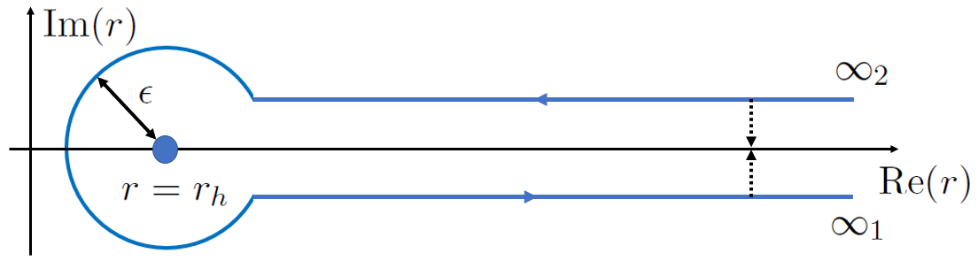
Figure 1: The holographic SK contour of Glorioso:2018mmw : the complexified radial coordinate analytically continued around the event horizon $r=r_{h}$. The dashed arrows indicate that the horizontal segments are infinitesimally close to the real axis.

The two ends of the $r$ contour are identified with the SK contour of the boundary theory Kamenev2011 ; Calzetta-Hu2009 , the infinitesimally small horizon circle is mapped into initial thermal state, while the horizontal segments reflect the CTP. The holographic contour of Figure 1 is obtained by taking two exteriors of an eternal AdS₅ black hole Maldacena:2001kr and identifying their future horizons.

The EF time $v$ is related to the Schwarzschild time $t$ by

$$t=v-\zeta_{2}(r),\qquad\zeta_{2}(r)\equiv\int_{\infty_{2}}^{r}\frac{dy}{f(y)},\qquad r\in[r_{h}-\epsilon,\infty_{2}),$$

$$t=v-\zeta_{1}(r),\qquad\zeta_{1}(r)\equiv\int_{\infty_{1}}^{r}\frac{dy}{f(y)},\qquad r\in[r_{h}-\epsilon,\infty_{1}),$$ (30)

where the integration constants are fixed by requirement that $t$ and $v$ coincide on the AdS boundaries. An interesting observation is that viewed in the ingoing EF coordinate (that is the EF time $v$ is identical everywhere along the radial contour), the Schwarzschild time $t$ is discontinuous at $r=r_{h}-\epsilon$,

$$t^{\rm up}(r_{h}-\epsilon)-t^{\rm dw}(r_{h}-\epsilon)=\int_{\infty_{1}}^{\infty_{2}}\frac{dy}{f(y)}=-\frac{i\pi}{2r_{h}}=-\frac{i\beta}{2},$$ (31)

where $\beta$ is inverse of the black brane temperature $T$. This becomes important when gluing bulk fields of the upper and lower segments of the contour in Figure 1.

3.2 Maxwell field in the bulk

The holographic model for the $U(1)$ diffusion is a probe Maxwell field in the above described geometry. The bulk action is

$$S_{0} =-\frac{1}{4}\int d^{4}x\int_{\infty_{2}}^{\infty_{1}}dr\sqrt{-g}F_{MN}F^{MN}$$ (32)

$$=-\frac{1}{4}\int d^{4}\tilde{x}\int_{\infty_{2}}^{\infty_{1}}dr\sqrt{-\tilde{g}}\tilde{F}_{MN}\tilde{F}^{MN},$$ (33)

where $C_{N}$ and $\tilde{C}_{N}$ are the $U(1)$ bulk gauge fields in EF and Schwarzschild coordinate systems respectively; $F_{MN}=\nabla_{M}C_{N}-\nabla_{N}C_{M}$ and $\tilde{F}_{MN}=\tilde{\nabla}_{M}\tilde{C}_{N}-\tilde{\nabla}_{N}\tilde{C}_{M}$. To remove the UV divergences near the AdS boundaries $r=\infty_{1}$ and $r=\infty_{2}$, the bulk action (32) (or (33)) should be supplemented with a counter-term action:

$$S_{\rm c.t.}=\frac{1}{4}\log r\int d^{4}x\sqrt{-\gamma}F_{\mu\nu}F^{\mu\nu}\bigg{|}_{r=\infty_{1}}-\frac{1}{4}\log r\int d^{4}x\sqrt{-\gamma}F_{\mu\nu}F^{\mu\nu}\bigg{|}_{r=\infty_{2}},$$ (34)

where the indices are contracted with the induced metric $\gamma_{\mu\nu}$

$$ds^{2}|_{\Sigma}=\gamma_{\mu\nu}dx^{\mu}dx^{\nu}=-f(r)dv^{2}+r^{2}\delta_{ij}dx^{i}dx^{j}.$$ (35)

Here $\Sigma$ denotes either the hypersurface $r=\infty_{1}$ or $r=\infty_{2}$. The counter-term action in the Schwarzschild coordinate system is the same as (34), since $v=t$ at the AdS boundaries. The minimal subtraction scheme (34) differs from that used in Glorioso:2018mmw .

Transformation rule for the fields from the EF coordinate system to the Schwarzschild can be easily derived from the coordinate-invariants

$$\tilde{C}_{M}d\tilde{x}^{M}=C_{M}dx^{M},$$ (36)

leading to

$$\tilde{C}_{t}(r,t,\vec{x})=C_{v}(r,v,\vec{x}),\qquad\tilde{C}_{i}(r,t,\vec{x})=C_{i}(r,v,\vec{x}).$$ (37)

The radial components of the bulk gauge field differ

$$\tilde{C}_{r}(r,t,\vec{x})-\frac{\tilde{C}_{t}(r,t,\vec{x})}{f(r)}=C_{r}(r,v,\vec{x})\Longrightarrow\tilde{C}_{r}(r,t,\vec{x})=C_{r}(r,v,\vec{x})+\frac{C_{v}(r,v,\vec{x})}{f(r)}.$$ (38)

Thus it is important to distinguish between two radial gauge choices:

$${\rm Schwarzschild~{}radial~{}gauge}:\qquad \tilde{C}_{r}=0\Longleftrightarrow C_{r}=-\frac{C_{v}}{f(r)},$$

$${\rm EF~{}radial~{}gauge}:\qquad C_{r}=0\Longleftrightarrow\tilde{C}_{r}=\frac{\tilde{C}_{t}}{f(r)}.$$ (39)

The EF radial gauge is most commonly used, including in Glorioso:2018mmw . Yet, for reasons related to time-reversal symmetry which will be explained in the next section, we chose to perform calculations in the Schwarzschild radial gauge.

Bulk EOMs are derived by variation of (32) and (33):

$$\nabla_{M}F^{MN}=0\Longrightarrow\frac{1}{\sqrt{-g}}\partial_{M}(\sqrt{-g}F^{MN})=0,$$ (40)

$$\tilde{\nabla}_{M}\tilde{F}^{MN}=0\Longrightarrow\frac{1}{\sqrt{-\tilde{g}}}\tilde{\partial}_{M}(\sqrt{-\tilde{g}}\tilde{F}^{MN})=0.$$ (41)

With the help of (37) and (38), the two sets of the Maxwell equations can be related

$$\tilde{\nabla}_{M}\tilde{F}^{Mr}=\nabla_{M}F^{Mr},\quad\tilde{\nabla}_{M}\tilde{F}^{Mt}=\nabla_{M}F^{Mv}-\frac{1}{f(r)}\nabla_{M}F^{Mr},~{}~{}~{}\tilde{\nabla}_{M}\tilde{F}^{Mi}=\nabla_{M}F^{Mi}.$$ (42)

The first equation (the $r$-component) is a gauge invariant constraint, which will play a special role in our construction. When all the bulk equations are solved (i.e., on-shell holography), (40) and (41) are absolutely equivalent as is obvious from (42). Yet, in Bu:2015ame we argued that in order to compute the TCFs parameterising the (off-shell) constitutive relations for the current, it is sufficient to solve the bulk dynamical equations only, while leaving the constraint aside. Within the holographic prescription the constraint is mapped into continuity equation for the current at the boundary, which is the dynamical equation for the low energy modes $\varphi_{1}$ and $\varphi_{2}$. Derivation of the effective action follows the very same strategy as introduced in Bu:2014sia ; Bu:2014ena ; Bu:2015ika ; Bu:2015ame , now frequently referred to as off-shell holography Crossley:2015tka ; deBoer:2015ija .

We are going to solve the EOMs in the Schwarzschild coordinates and then re-express the results in the EF coordinates using (37) and (38). In the spirit of the off-shell formalism, we will not impose the constraint equation. Hence, the dynamical equations which will be solved are

$$\nabla_{M}F^{Mv}-\frac{1}{f(r)}\nabla_{M}F^{Mr}=0\Longleftrightarrow\tilde{\nabla}_{M}\tilde{F}^{Mt}=0,\qquad\nabla_{M}F^{Mi}=0\Longleftrightarrow\tilde{\nabla}_{M}\tilde{F}^{Mi}=0.$$ (43)

Notice that the first equation differs from $\nabla_{M}F^{Mv}=0$ derived in the EF coordinates. The seemingly freedom to modify the dynamical equation is eliminated when the Schwarzschild radial gauge is implemented in the effective action.

We will find the Bianchi identity Glorioso:2018mmw is quite useful:

$$\partial_{r}(\sqrt{-g}\nabla_{M}F^{Mr})+\partial_{v}(\sqrt{-g}\nabla_{M}F^{Mv})+\partial_{k}(\sqrt{-g}\nabla_{M}F^{Mk})=0.$$ (44)

The dynamical equations (43) are instrumental in deriving a holographic RG flow-like equation for $\nabla_{M}F^{Mr}$:

$$\partial_{r}\left(\sqrt{-g}\nabla_{M}F^{Mr}\right)=\frac{i\omega}{f(r)}\sqrt{-g}\nabla_{M}F^{Mr},$$ (45)

which is solved by

$$\sqrt{-g}\nabla_{M}F^{Mr}=\mathcal{C}^{\rm up}(k)e^{i\omega\zeta_{2}(r)},\qquad r\in[r_{h}-\epsilon,\infty_{2}),$$

$$\sqrt{-g}\nabla_{M}F^{Mr}=\mathcal{C}^{\rm dw}(k)e^{i\omega\zeta_{1}(r)},\qquad r\in[r_{h}-\epsilon,\infty_{1}).$$ (46)

Here, $\mathcal{C}^{\rm up,\,dw}$ are $r$-independent integration constants in either upper or lower segments of the $r$-contour. Both vanish on-shell.

3.3 Boundary effective action

The basic procedure of how to derive a hydrodynamic effective action from gravity has been realized in Crossley:2015tka (see also Glorioso:2018mmw ), based on early attempts of formulating a holographic Wilsonian RG flow Heemskerk:2010hk ; Faulkner:2010jy . It amounts to identifying hydrodynamical variables (gapless modes) of the boundary theory, as proposed in Nickel:2010pr . The remaining degrees of freedom are then integrated out from the bulk action, in Wilsonian sense. The procedure is outlined below for a free $U(1)$ gauge field in the bulk.

The starting point is the bulk partition function:

$$Z=\int DC_{r}DC_{\mu}e^{iS_{0}[C_{\mu},C_{r}]+iS_{\rm c.t.}}.$$ (47)

No gauge-fixing has been applied at this stage. Integrating by parts, the bulk action $S_{0}$ (32) can be expressed as

$$S_{0}= -\frac{1}{2}\int d^{4}x\int_{\infty_{2}}^{\infty_{1}}dr\sqrt{-g}\left[\nabla_{M}\left(C_{N}F^{MN}\right)-C_{N}\nabla_{M}F^{MN}\right]$$

$$= \frac{1}{2}\int d^{4}x\int_{\infty_{2}}^{\infty_{1}}dr\sqrt{-g}\left[C_{r}\nabla_{M}F^{Mr}+C_{v}\nabla_{M}F^{Mv}+C_{k}\nabla_{M}F^{Mk}\right]$$

$$-\frac{1}{2}\int d^{4}x\sqrt{-\gamma}n_{M}C_{N}F^{MN}\bigg{|}_{r=\infty_{2}}^{r=\infty_{1}}$$

$$= \frac{1}{2}\int d^{4}x\int_{\infty_{2}}^{\infty_{1}}dr\sqrt{-g}\left\{C_{v}\left[\nabla_{M}F^{Mv}-\frac{1}{f(r)}\nabla_{M}F^{Mr}\right]+C_{k}\nabla_{M}F^{Mk}\right.$$

$$\left.+\left(C_{r}+\frac{C_{v}}{f(r)}\right)\nabla_{M}F^{Mr}\right\}-\frac{1}{2}\int d^{4}x\sqrt{-\gamma}n_{M}C_{N}F^{MN}\bigg{|}_{r=\infty_{2}}^{r=\infty_{1}},$$ (48)

where $n_{M}$ is a out-pointing unit vector normal to the hypersurface $\Sigma$.

Our goal now is to derive the effective action. We will demonstrate how the bulk gauge invariance is realised. Our derivation is an explicit holographic construction that closely follows the original ideas of Crossley:2015evo .

The discussion below applies separately to each segment of the contour. The asymptotic values of the gauge field are identified with the boundary external background field $\mathcal{A}_{\mu}$,

$$C_{\mu}(r=\infty,x^{\alpha})\equiv\mathcal{A}_{\mu}.$$ (49)

Consider a generic gauge transformation parameterised by $\Lambda(r,x^{\alpha})$ transforming the bulk gauge field $C_{M}$ as

$$C_{\mu}\to C_{\mu}^{\prime}=C_{\mu}+\partial_{\mu}\Lambda(r,x^{\alpha}),\qquad C_{r}\to C_{r}^{\prime}=C_{r}+\partial_{r}\Lambda(r,x^{\alpha}).$$ (50)

In the path integral (47), the gauge transformation (50) can be viewed as a change of integration variables, say, from $C_{r}$ to $\Lambda$. In other words, the gauge transformation defines a map from any given configuration of $C_{r}$ into a configuration with some fixed radial gauge. For example, for $C_{M}^{\prime}$ to be in the EF radial gauge,

$$C_{r}^{\prime}=0\Rightarrow\Lambda(r,x^{\alpha})=\int_{r}^{r_{c}}d\xi C_{r}(\xi,x^{\alpha}).$$ (51)

The boundary value of $C_{\mu}^{\prime}$:

$$C_{\mu}^{\prime}(r=\infty,x^{\alpha})=\mathcal{A}_{\mu}+\partial_{\mu}\varphi,$$ (52)

where $\varphi\equiv\Lambda(r=\infty,x^{\alpha})$ is identified with the hydrodynamic field associated with the $U(1)$ charge. $\Lambda$ can be similarly constructed for the Schwarzschild radial gauge $C_{r}^{\prime}=-C_{v}^{\prime}/f(r)$.

Integration over $C_{\mu}$ in (47) can be performed in the saddle point approximation, which is exact for the Maxwell theory. That is, solutions of the dynamical equations for $C_{\mu}$ are plugged into $S_{0}[C_{\mu},C_{r}]$. As long as no radial gauge is imposed, $C_{\mu}$ are functionals of $C_{r}$. Generically, the partition function (47) turns into

$$Z=\int DC_{r}e^{iS_{0}[C_{\mu}[C_{r}],C_{r}]+iS_{\rm c.t.}},$$ (53)

where $S_{0}[C_{\mu}[C_{r}],C_{r}]$ is a “partially on-shell” bulk action deBoer:2015ija which depends on $C_{r}$ both explicitly and through solutions for $C_{\mu}$. The action is gauge invariant. Since in practice $C_{\mu}[C_{r}]$ are computed in a fixed gauge, the next step is to fix the gauge using (50), while changing the integration variable from $C_{r}$ to $\Lambda$. The resulting partially on-shell action does not depend on the whole $\Lambda$ but on $\varphi$ only. (53) becomes

$$Z\sim\int D\varphi e^{iS_{0}|_{\rm p.o.s.}+iS_{\rm c.t.}}$$ (54)

where $S_{0}|_{\rm p.o.s.}+S_{\rm c.t.}$ is the boundary effective action $S_{eff}$ of the $\varphi$ field. Here, an overall coefficient due to Jacobian of the change of variables has been absorbed into $D\varphi$ measure. Below we will explicitly derive $S_{0}|_{\rm p.o.s.}$ for the EF radial gauge $C_{r}^{\prime}=0$ and Schwarzschild radial gauge $C_{r}^{\prime}=-C_{v}^{\prime}/f(r)$, and demonstrate the equivalence of the results. In fact, it is straightforward to show that the result for $S_{0}|_{\rm p.o.s.}$ is independent of the gauge-fixing.

In the EF radial gauge $C_{r}^{\prime}=0$, the partially on-shell bulk action is evaluated as

$$S_{0}|_{\rm p.o.s} =\frac{1}{2}\int d^{4}x\int_{\infty_{2}}^{\infty_{1}}dr\sqrt{-g}C_{r}\nabla_{M}F^{Mr}-\frac{1}{2}\int d^{4}x\sqrt{-\gamma}n_{M}C_{N}F^{MN}\bigg{|}_{r=\infty_{2}}^{r=\infty_{1}}$$

$$=\frac{1}{2}\int d^{4}x\int_{\infty_{2}}^{\infty_{1}}dr\sqrt{-g}(-\partial_{r}\Lambda)\nabla_{M}F^{Mr}-\frac{1}{2}\int d^{4}x\sqrt{-\gamma}n_{M}C_{N}F^{MN}\bigg{|}_{r=\infty_{2}}^{r=\infty_{1}}$$

$$=\frac{1}{2}\int d^{4}x\left[-\sqrt{-g}\Lambda\nabla_{M}F^{Mr}-\sqrt{-\gamma}n_{M}C_{N}F^{MN}\right]\bigg{|}_{r=\infty_{2}}^{r=\infty_{1}}$$

$$=-\frac{1}{2}\int d^{4}x\sqrt{-g}C_{\mu}^{\prime}F^{r\mu}[C_{\mu}^{\prime},C_{r}^{\prime}=0]\bigg{|}_{r=\infty_{2}}^{r=\infty_{1}}.$$ (55)

Similarly, in the Schwarzschild radial gauge $C_{r}^{\prime}=-C_{v}^{\prime}/f(r)$, the partially on-shell bulk action is calculated as

$$S_{0}|_{\rm p.o.s} =\frac{1}{2}\int d^{4}x\int_{\infty_{2}}^{\infty_{1}}dr\sqrt{-g}\left(C_{r}+\frac{C_{v}}{f(r)}\right)\nabla_{M}F^{Mr}-\frac{1}{2}\int d^{4}x\sqrt{-\gamma}n_{M}C_{N}F^{MN}\bigg{|}_{r=\infty_{2}}^{r=\infty_{1}}$$

$$=-\frac{1}{2}\int d^{4}x\int_{\infty_{2}}^{\infty_{1}}dr\sqrt{-g}\left(\partial_{r}\Lambda+\frac{\partial_{v}\Lambda}{f(r)}\right)\nabla_{M}F^{Mr}-\frac{1}{2}\int d^{4}x\sqrt{-\gamma}n_{M}C_{N}F^{MN}\bigg{|}_{r=\infty_{2}}^{r=\infty_{1}}$$

$$=-\frac{1}{2}\int d^{4}x\int_{\infty_{2}}^{\infty_{1}}dr\left(\partial_{r}+\frac{\partial_{v}}{f(r)}\right)\left[\Lambda\sqrt{-g}\nabla_{M}F^{Mr}\right]-\frac{1}{2}\int d^{4}x\sqrt{-\gamma}n_{M}C_{N}F^{MN}\bigg{|}_{r=\infty_{2}}^{r=\infty_{1}}$$

$$=\frac{1}{2}\int d^{4}x\int_{\infty_{2}}^{\infty_{1}}dr\left[-\Lambda\sqrt{-g}\nabla_{M}F^{Mr}-\sqrt{-\gamma}n_{M}C_{N}F^{MN}\right]\bigg{|}_{r=\infty_{2}}^{r=\infty_{1}}$$

$$=-\frac{1}{2}\int d^{4}x\sqrt{-g}C_{\mu}^{\prime}F^{r\mu}[C_{\mu}^{\prime},C_{r}^{\prime}=-C_{v}^{\prime}/f(r)]\bigg{|}_{r=\infty_{2}}^{r=\infty_{1}}.$$ (56)

Both in (55) and (56), the terms representing the total derivatives at the AdS boundaries were dropped. The Bianchi identity (44) was instrumental to convert the bulk integral into the surface term. Gauge invariance of the field strength $F^{MN}[C_{\mu},C_{r}]=F^{MN}[C_{\mu}^{\prime},C_{r}^{\prime}]$ was used as well. (55) and (56) are identical and become a superposition of two surface terms

$$S_{0}|_{\rm p.o.s.}=-\frac{1}{2}\int d^{4}x\sqrt{-\gamma}n_{M}C_{N}^{\prime}F^{MN}[C_{\mu}^{\prime},C_{r}^{\prime}]\bigg{|}_{r=\infty_{2}}^{r=\infty_{1}}.$$ (57)

Notice that (57) could be obtained from (a primed version of) (48) by dropping all the bulk terms, either because of the dynamical equations (43) or as a result of the Schwarzschild radial gauge.

There is a subtle point in deriving (57). As will become clear in the next section, in the off-shell formalism, the gauge potential and/or field strength develop discontinuity near the event horizon. Hence, in principle, there might emerge an additional boundary term at the horizon surface. This term will be eliminated by a specific choice of the boundary conditions to be discussed below.

Below we will drop the prime in $C_{M}^{\prime}$ and permanently stick to the Schwarzschild radial gauge for $C_{M}$. The bulk EOMs (43) will be solved subject to boundary conditions at two AdS boundaries $r=\infty_{1}$ and $r=\infty_{2}$:

$$C_{\mu}\xrightarrow[]{r\to\infty_{1}}B_{1\mu}(x^{\alpha})\equiv\mathcal{A}_{1\mu}+\partial_{\mu}\varphi_{1},\qquad\qquad C_{\mu}\xrightarrow[]{r\to\infty_{2}}B_{2\mu}(x^{\alpha})\equiv\mathcal{A}_{2\mu}+\partial_{\mu}\varphi_{2}.$$ (58)

In order to compute the boundary action (57), near boundary asymptotic expansion of the bulk fields is required. It has the form

$$C_{\mu}\xrightarrow[]{r\to\infty_{1}}B_{1\mu}(x^{\alpha})+\frac{\partial_{v}B_{1\mu}(x^{\alpha})}{r}-\frac{1}{2}\partial^{\nu}\mathcal{F}_{1\mu\nu}(x^{\alpha})\frac{\log r}{r^{2}}+\frac{C_{1\mu}^{(2)}(x^{\alpha})}{r^{2}}+\cdots,$$ (59)

$$C_{\mu}\xrightarrow[]{r\to\infty_{2}}B_{2\mu}(x^{\alpha})+\frac{\partial_{v}B_{2\mu}(x^{\alpha})}{r}-\frac{1}{2}\partial^{\nu}\mathcal{F}_{2\mu\nu}(x^{\alpha})\frac{\log r}{r^{2}}+\frac{C_{2\mu}^{(2)}(x^{\alpha})}{r^{2}}+\cdots,$$ (60)

where the coefficient functions $C_{1\mu}^{(2)}$ and $C_{2\mu}^{(2)}$ are functionals of both $B_{1\mu}$ and $B_{2\mu}$. They will be determined through the solution of the dynamical equations (43) over the entire contour in Figure. 1. This is the subject of the next section.

Once (59) and (60) are substituted into the total action $S_{\rm eff}=S_{0}|_{\rm p.o.s.}+S_{\rm c.t.}$, the latter takes the form (4) with the effective Lagrangian $\mathcal{L}_{\rm eff}(x)$ being a quadratic functional of the boundary fields $B_{1\mu}$ and $B_{2\mu}$ (in the $(r,a)$-basis)

$$\mathcal{L}_{\rm eff}= -B_{rv}(C_{1v}^{(2)}-C_{2v}^{(2)})-\frac{1}{2}B_{av}(C_{1v}^{(2)}+C_{2v}^{(2)})+B_{rk}(C_{1k}^{(2)}-C_{2k}^{(2)})$$

$$+\frac{1}{2}B_{ak}(C_{1k}^{(2)}+C_{2k}^{(2)}){+\frac{1}{2}\partial_{k}B_{ak}\partial_{v}B_{rv}-\frac{1}{2}B_{av}\partial_{v}\partial_{k}B_{rk}}$$

$$-\frac{1}{2}B_{ak}\partial_{v}^{2}B_{rk}+\frac{1}{4}\mathcal{F}_{akj}\mathcal{F}_{rkj}+\frac{1}{2}B_{av}\vec{\partial}^{\,2}B_{rv}{+B_{av}\partial_{v}^{2}B_{rv}}.$$ (61)

With the help of a basis decomposition procedure introduced in Bu:2015ame , the effective Lagrangian (61) can be recast into the form (2.1), thus providing a holographic derivation of the latter, which is fully consistent with the general analysis of Crossley:2015evo . This derivation is presented in Appendix A.

4 Bulk dynamics: solutions and analysis

This section is devoted to solutions of the bulk EOMs (43) over the contour displayed in Figure 1. Our strategy will be different from that of Glorioso:2018mmw . Instead of integrating the bulk EOMs (43) along the entire $r$-contour, we split the radial contour at $r=r_{h}-\epsilon$ into two segments, the upper and lower one. Each segment “lives” in a single copy of the doubled Schwarzschild-AdS₅ geometry. In each segment, there is a set of independent solutions to the dynamical EOMs (43) forming a basis. Full solutions obeying the respective boundary conditions (58) will be constructed as linear superpositions of the basis solutions. Thus-constructed piecewise solutions will be carefully glued at the cutting slice $r=r_{h}-\epsilon$, under proper matching conditions to be derived in subsection 4.2. One of the advantages of our approach is that it avoids the subtleties related to non-commutativity between two limits: the hydrodynamic derivative expansion and $\epsilon\rightarrow 0$, the latter has to be taken first.

4.1 Discrete symmetries

Symmetries in classical theories are used in order to generate solutions, if one is already known. Maxwell’s theory in the bulk (single copy Schwarzschild-AdS) has a number of discrete symmetries, such as parity and time reversal, which will be employed in our quest after a full set of independent solutions. However, in different coordinate systems, the symmetries are represented differently. Particularly, while in the Schwarzschild coordinates the time reversal symmetry is realised trivially, its representation in the EF coordinates is much less transparent. This is essentially the main reason we have chosen to first find all the solutions in the Schwarzschild coordinates and then translate those into the EF system.

In the Schwarzschild coordinates (without any gauge fixing yet), the Fourier mode $\tilde{C}_{M}(r,k^{\mu})$ defined by

$$\tilde{C}_{M}(r,t,x^{i})=\int\frac{d^{4}k}{(2\pi)^{4}}e^{ik\cdot x}\tilde{C}_{M}(r,k^{\mu}),\qquad k^{\mu}=(\omega,\vec{q}),$$ (62)

satisfies the following system of ODEs:

$$\tilde{\nabla}_{M}\tilde{F}^{Mr}=0\Rightarrow 0= (i\omega\partial_{r}\tilde{C}_{t}-\omega^{2}\tilde{C}_{r})+r^{-2}f(r)(q^{2}\tilde{C}_{r}+iq_{k}\partial_{r}\tilde{C}_{k}),$$ (63)

$$\tilde{\nabla}_{M}\tilde{F}^{Mt}=0\Rightarrow 0= \partial_{r}(r^{3}\partial_{r}\tilde{C}_{t})+i\omega\partial_{r}(r^{3}\tilde{C}_{r})-\frac{r}{f(r)}(q^{2}\tilde{C}_{t}+\omega q_{k}\tilde{C}_{k}),$$ (64)

$$\tilde{\nabla}_{M}\tilde{F}^{Mi}=0\Rightarrow 0= \partial_{r}[rf(r)\partial_{r}\tilde{C}_{i}]-iq_{i}\partial_{r}[rf(r)\tilde{C}_{r}]+\frac{r}{f(r)}(\omega^{2}\tilde{C}_{i}+\omega q_{i}\tilde{C}_{t})$$

$$+r^{-1}(-q^{2}\tilde{C}_{i}+q_{i}q_{k}\tilde{C}_{k}).$$ (65)

The full set of bulk EOMs (63)-(65) is obviously invariant under the following time-reversal transformation:

$$\omega\to-\omega,\qquad\tilde{C}_{t}(r,k^{\mu})\to\tilde{C}_{t}(r,\bar{k}^{\mu}),\qquad\tilde{C}_{i}(r,k^{\mu})\to-\tilde{C}_{i}(r,\bar{k}^{\mu}),$$

$$\tilde{C}_{r}(r,k^{\mu})\to-\tilde{C}_{r}(r,\bar{k}^{\mu}),\qquad\qquad{\rm with}~{}~{}\bar{k}^{\mu}=(-\omega,\vec{q}),$$ (66)

which, in the coordinate space $(r,t,\vec{x})$, turns into

$$t\to-t,\qquad\tilde{C}_{t}(r,t,\vec{x})\to\tilde{C}_{t}(r,-t,\vec{x}),\qquad\tilde{C}_{i}(r,t,\vec{x})\to-\tilde{C}_{i}(r,-t,\vec{x}),$$

$$\tilde{C}_{r}(r,t,\vec{x})\to-\tilde{C}_{r}(r,-t,\vec{x}).$$ (67)

Furthermore, the dynamical EOMs (64) and (65) are invariant under the time reversal independently, regardless of the constraint equation (63) being imposed or not. Transformations (4.1) and (4.1) can be recognised as a linear realisation of the time-reversal symmetry Chakrabarty:2019aeu .

In the ingoing EF coordinates (28), the Fourier mode $C_{M}(r,k^{\mu})$ defined by

$$C_{M}(r,x^{\mu})=\int\frac{d^{4}k}{(2\pi)^{4}}e^{ik\cdot x}C_{M}(r,k^{\mu}),\qquad k^{\mu}=(\omega,\vec{q}),$$ (68)

obeys another system of ODEs:

$$\nabla_{M}F^{Mr}=0~{}\Rightarrow~{}0=r^{3}(\omega^{2}C_{r}-i\omega\partial_{r}C_{v})-rf(r)(q^{2}C_{r}+iq_{k}\partial_{r}C_{k})-r(q^{2}C_{v}+\omega q_{k}C_{k}),$$ (69)

$$\nabla_{M}F^{Mv}-\frac{1}{f(r)}\nabla_{M}F^{Mr}=0~{}\Rightarrow~{}0=\partial_{r}(r^{3}\partial_{r}C_{v}+i\omega r^{3}C_{r})+r(q^{2}C_{r}+iq_{k}\partial_{r}C_{k})$$

$$~{}~{}~{}~{}~{}~{}~{}~{}~{}~{}~{}~{}~{}~{}~{}~{}~{}~{}~{}+\frac{r^{3}}{f(r)}(\omega^{2}C_{r}-i\omega\partial_{r}C_{v})-\frac{r}{f(r)}(q^{2}C_{v}+\omega q_{k}C_{k})-r(q^{2}C_{r}+iq_{k}\partial_{r}C_{k}),$$ (70)

$$\nabla_{M}F^{Mi}=0~{}\Rightarrow~{}0=\partial_{r}[rf(r)(\partial_{r}C_{i}-iq_{i}C_{r})]-\partial_{r}[r(i\omega C_{i}+iq_{i}C_{v})]$$

$$~{}~{}~{}~{}~{}~{}~{}~{}~{}~{}~{}~{}~{}~{}~{}~{}~{}~{}~{}~{}~{}~{}~{}~{}~{}~{}~{}~{}~{}~{}~{}~{}~{}~{}~{}~{}~{}~{}~{}~{}~{}~{}~{}~{}~{}~{}-r(i\omega\partial_{r}C_{i}+\omega q_{i}C_{r})+r^{-1}(-q^{2}C_{i}+q_{i}q_{k}C_{k}).$$ (71)

Apparently, the transformation like (4.1) is not a symmetry of EOMs (69)-(71). This is related to the fact that $v\to-v$ is not a symmetry, because the transformation does not leave the metric (28) invariant. This point was made clear in Chakrabarty:2019aeu , which carried out a somewhat similar analysis of a probe string in Schwarzschild-AdS background.

What is a nonlinear realisation of the underlying time-reversal symmetry in the ingoing EF coordinates? This could be worked out with the help of (37) and (38). The Fourier modes in the Schwarzschild and ingoing EF coordinates are related,

$$C_{\mu}(r,k)=\tilde{C}_{\mu}(r,k)e^{i\omega\zeta_{s}(r)},\qquad C_{r}(r,k)=\left[\tilde{C}_{r}(r,k)-\frac{\tilde{C}_{t}(r,k)}{f(r)}\right]e^{i\omega\zeta_{s}(r)},$$

$$r\in[r_{h}-\epsilon,\infty_{s}),\qquad s=1~{}{\rm or}~{}2,$$ (72)

where $\zeta_{1}(r)$ and $\zeta_{2}(r)$ are introduced in (30). Thus, in the ingoing EF coordinates, the time-reversal symmetry is realized as

$$\omega\to-\omega,\quad C_{v}(r,k)\to C_{v}(r,\bar{k})e^{2i\omega\zeta_{s}(r)},\quad C_{i}(r,k)\to-C_{i}(r,\bar{k})e^{2i\omega\zeta_{s}(r)},$$

$$C_{r}(r,k)\to-\left[C_{r}(r,\bar{k})+\frac{2C_{v}(r,\bar{k})}{f(r)}\right]e^{2i\omega\zeta_{s}(r)},\qquad s=1,2.$$ (73)

So far, no gauge choice has been specified. In Glorioso:2018mmw , the EF radial gauge $C_{r}=0$ was chosen, which is in tension with the linear realisation of the time-reversal symmetry (4.1). In fact, a time reversed solution is gauge transformed with respect to $C_{r}=0$. Hence, in order to benefit from the simplicity of (4.1), we search for solutions in the Schwarzschild radial gauge $\tilde{C}_{r}=0$.

The bulk EOMs (63)-(65) are also invariant under $\mathcal{P}$-symmetry (space inversion):

$$\vec{q}\to-\vec{q},\qquad\tilde{C}_{t}(r,k^{\mu})\to\tilde{C}_{t}(r,-\bar{k}^{\mu}),\qquad\tilde{C}_{i}(r,k^{\mu})\to-\tilde{C}_{i}(r,-\bar{k}^{\mu}),$$

$$~{}~{}~{}~{}~{}~{}~{}~{}~{}~{}~{}~{}\tilde{C}_{r}(r,k^{\mu})\to\tilde{C}_{r}(r,-\bar{k}^{\mu}),$$ (74)

or, alternatively, in the coordinate space $(r,t,\vec{x})$

$$\vec{x}\to-\vec{x},\qquad\tilde{C}_{t}(r,t,\vec{x})\to\tilde{C}_{t}(r,t,-\vec{x}),\qquad\tilde{C}_{i}(r,t,\vec{x})\to-\tilde{C}_{i}(r,t,-\vec{x}),$$

$$~{}~{}~{}~{}~{}~{}~{}~{}~{}~{}~{}~{}~{}\tilde{C}_{r}(r,t,\vec{x})\to\tilde{C}_{r}(r,t,-\vec{x}).$$ (75)

Since the coordinate transformation from (28) to (29) does not involve spatial directions, the $\mathcal{P}$-symmetry in the EF coordinates takes exactly the same form as (74) and (75), which can be straightforwardly checked from the bulk EOMs (69)-(71).

The time-reversal $\mathcal{T}$ symmetry and $\mathcal{P}$-symmetry help to examine the symmetry relations for TCFs in the effective action, as reviewed in subsection 2.2.

4.2 Horizon matching conditions

As has been already mentioned, we first derive independent solutions in the upper and lower segments, and then glue them at the surface $r=r_{h}-\epsilon$. In this way a complete solution valid along the whole radial contour in Figure 1 is constructed. A necessary element of this construction is a set of matching conditions for the bulk fields to be discussed in this subsection.

The contour in Figure 1 is cut along the surface $r=r_{\pm}\equiv r_{h}-\epsilon$, where the subscripts ₊ and _- are used to distinguish the upper and lower segments. In the spirit of Skenderis:2008dg , the matching conditions at $r=r_{h}-\epsilon$ can be obtained by demanding the total bulk action to be extremal with respect to variation of the horizon data $C_{M}(r_{h}-\epsilon,x^{\mu})$. Consider variation of the bulk action (32)

$$\delta S_{0}= -\int d^{4}x\sqrt{-\gamma}n_{M}\delta C_{N}F^{MN}\bigg{|}_{r_{-}}^{\infty_{1}}+\int d^{4}x\sqrt{-\gamma}n_{M}\delta C_{N}F^{MN}\bigg{|}_{r_{+}}^{\infty_{2}}$$

$$+\int d^{4}x\int_{\infty_{2}}^{\infty_{1}}dr\sqrt{-g}\left[\delta C_{r}\nabla_{M}F^{Mr}+\delta C_{v}\frac{\nabla_{M}F^{Mr}}{f(r)}\right]$$ (76)

where we imposed the dynamical equations (43). The extremum condition (at the surface $r=r_{h}-\epsilon$) gives

$$\frac{\delta S}{\delta C_{v}(r_{h}-\epsilon)}=0\Rightarrow F^{rv}(r_{+})-F^{rv}(r_{-})=\lim_{\Delta\to 0}\int_{r_{+}+\Delta}^{r_{-}-\Delta}dr\frac{\nabla_{M}F^{Mr}}{f(r)},$$ (77)

$$\frac{\delta S}{\delta C_{i}(r_{h}-\epsilon)}=0\Rightarrow F^{ri}(r_{+})-F^{ri}(r_{-})=0,$$ (78)

where $\Delta$ is an infinitesimal interval along the circle in Figure 1. The field strength components $F^{ri}$ are continuous through the cutting surface. Yet, the $F^{rv}$ component, being continuous for on-shell theory, may develop discontinuity if the constraint equation is relaxed, that is, $\nabla_{M}F^{Mr}\neq 0$. When implementing the Schwarzschild radial gauge $\tilde{C}_{r}=0$, the matching condition (78) translates into

$$f(r)\partial_{r}C_{i}\big{|}_{r=r_{+}}=f(r)\partial_{r}C_{i}\big{|}_{r=r_{-}}.$$ (79)

Since $f(r)$ vanishes at the horizon, $\partial_{r}C_{i}$ may not be continuous. Similarly, $C_{r}$ component is discontinuous.

The condition (77) is very non-trivial. It suggests that $\partial_{r}C_{v}$ is discontinuous too. Yet, this conclusion is based on assumption that $C_{\mu}$ is continuous across the cutting slice:

$$C_{\mu}(r_{-})=C_{\mu}(r_{+}).$$ (80)

(80) is a natural choice that could be realised via a residual gauge transformation implementable on each segment independently. Furthermore, thanks to the residual gauge freedom, we could set

$$C_{v}(r_{h}-\epsilon,x^{\mu})=0.$$ (81)

This choice has been also implemented in Glorioso:2018mmw , though through a somewhat different chain of arguments. Once the condition (81) is imposed, (77) fixes the discontinuity of $\partial_{r}C_{v}$ uniquely. Below we will construct the full solution of EOMs with the matching condition (81) and then check that (77) is indeed satisfied. This consistency check will be presented in Appendix B.

Finally, an added value of the choice (81) is that it makes the horizon contribution to the effective action $S_{0}$ vanish. Hence, (57) is correct .

4.3 Linearly independent solutions

In this subsection, we derive and analyse all linearly independent solutions of the dynamical EOMs (43) in a single Schwarzschild-AdS₅. The solutions are equally valid both in the upper and lower segments in Figure 1. As argued previously, in order to benefit from the linear realisation (4.1) of the time-reversal symmetry, we temporarily work in the Schwarzschild coordinate system combined with the Schwarzschild radial gauge. Eventually, linearly independent solutions in the ingoing EF coordinates will be deduced via the transformation rule (72). Without loss of generality, the spatial momentum $\vec{q}$ is taken to be along the $x$-direction. Then, the bulk fields $\tilde{C}_{\mu}$ decouple between two sectors: the transverse sector $\tilde{C}_{\perp}=\{\tilde{C}_{y},\tilde{C}_{z}\}$ and the longitudinal sector $\tilde{C}_{\parallel}=\{\tilde{C}_{t},\tilde{C}_{x}\}$.

Transverse sector.

The transverse mode $\tilde{C}_{\perp}$ obeys a single ODE:

$$0=\partial_{r}[rf(r)\partial_{r}\tilde{C}_{\perp}]+\frac{\omega^{2}r}{f(r)}\tilde{C}_{\perp}-q^{2}r^{-1}\tilde{C}_{\perp},\qquad\perp=y,z.$$ (82)

Eq. (82) has two independent solutions distinguishable by their near horizon behaviour.

Near the horizon $r=r_{h}$, the ingoing solution $\tilde{C}_{\perp}^{\rm ig}(r,k^{\mu})$ behaves as

$$\tilde{C}_{\perp}^{\rm ig}(r,k^{\mu})\xrightarrow[]{r\to r_{h}}(r-r_{h})^{-i\omega/(4r_{h})}\left[\tilde{C}_{\perp}^{h}+\tilde{C}_{\perp}^{1}(r-r_{h})+\tilde{C}_{\perp}^{2}(r-r_{h})^{2}+\cdots\right],$$ (83)

where $\tilde{C}_{\perp}^{h}$ is an integration constant (initial condition), which we refer to as horizon data. The remaining coefficients $\tilde{C}_{\perp}^{1},\tilde{C}_{\perp}^{2},\cdots$ are uniquely fixed in terms of $\tilde{C}_{\perp}^{h}$.

The outgoing solution $\tilde{C}_{\perp}^{\rm og}(r,k^{\mu})$ is obtained from the ingoing one by the time-reversal symmetry (4.1)

$$\tilde{C}_{\perp}^{\rm og}(r,k^{\mu})=-\tilde{C}_{\perp}^{\rm ig}(r,\bar{k}^{\mu}).$$ (84)

Both solutions are functions of $q^{2}$ as is obvious from (82), and hence they are $\mathcal{P}$-invariant. From (72), the solutions in the ingoing EF coordinates read:

$$C_{\perp}^{\rm ig}(r,k^{\mu})=\tilde{C}_{\perp}^{\rm ig}(r,k^{\mu})e^{i\omega\zeta_{s}(r)},\quad C_{\perp}^{\rm og}(r,k^{\mu})=\tilde{C}_{\perp}^{\rm og}(r,k^{\mu})e^{i\omega\zeta_{s}(r)},\quad r\in[r_{h}-\epsilon,\infty_{s}).$$ (85)

Thus, the ingoing and outgoing solutions are related to each other via

$$C_{\perp}^{\rm og}(r,k^{\mu})=-C_{\perp}^{\rm ig}(r,\bar{k}^{\mu})e^{2i\omega\zeta_{s}(r)},\qquad r\in[r_{h}-\epsilon,\infty_{s}),\qquad s=1~{}{\rm or}~{}2,$$ (86)

where (84) is used.

Near the AdS boundary the ingoing solution $C_{\perp}^{\rm ig}$ can be expanded

$$C_{\perp}^{\rm ig}(r,k^{\mu})\xrightarrow[]{r\to\infty} C_{\perp}^{\rm ig(0)}(k^{\mu})-\frac{i\omega C_{\perp}^{\rm ig(0)}(k^{\mu})}{r}+\frac{1}{2}(\omega^{2}-q^{2})C_{\perp}^{\rm ig(0)}(k^{\mu})\frac{\log r}{r^{2}}+\frac{C_{\perp}^{\rm ig(2)}(k^{\mu})}{r^{2}}+\cdots.$$ (87)

In principle, one could tune $\tilde{C}_{\perp}^{h}$ so that $C_{\perp}^{\rm ig(0)}(k^{\mu})=1$, though for a while we prefer to keep it unspecified.

Longitudinal sector.

The EOMs for the longitudinal sector $\tilde{C}_{\parallel}=\{\tilde{C}_{t},\tilde{C}_{x}\}$ are

$$0=\partial_{r}(r^{3}\partial_{r}\tilde{C}_{t})-\frac{r}{f(r)}(q^{2}\tilde{C}_{t}+\omega q\tilde{C}_{x}),$$

$$0=\partial_{r}[rf(r)\partial_{r}\tilde{C}_{x}]+\frac{r}{f(r)}(\omega^{2}\tilde{C}_{x}+\omega q\tilde{C}_{t}).$$ (88)

Compared to the transverse case, the coupling between $\tilde{C}_{t}$ and $\tilde{C}_{x}$ makes the longitudinal sector much more involved. The system of coupled equations (88) has four linearly independent solutions, which could be differentiated by their near horizon behaviour.

$\bullet$ The first solution is the ingoing solution $\{\tilde{C}_{t}^{\rm ig},\tilde{C}_{x}^{\rm ig}\}$,

$$\tilde{C}_{t}^{\rm ig}(r,k^{\mu})\xrightarrow[]{r\to r_{h}}(r-r_{h})^{1-i\omega/(4r_{h})}\left[\frac{4iq\tilde{C}_{x}^{{\rm ig}\,h}}{4r_{h}^{2}-i\omega r_{h}}+\cdots\right],$$

$$\tilde{C}_{x}^{\rm ig}(r,k^{\mu})\xrightarrow[]{r\to r_{h}}(r-r_{h})^{-i\omega/(4r_{h})}\left[\tilde{C}_{x}^{{\rm ig}\,h}+\frac{i\omega\tilde{C}_{x}^{{\rm ig}\,h}(8r_{h}^{2}+2i\omega r_{h}+\omega^{2}-4q^{2})}{8r_{h}^{2}(8r_{h}^{2}-6i\omega r_{h}-\omega^{2})}(r-r_{h})+\cdots\right],$$ (89)

where $\cdots$ are higher powers of $(r-r_{h})$. Both functions $\{\tilde{C}_{t}^{\rm ig},\tilde{C}_{x}^{\rm ig}\}$ are uniquely determined in terms of single horizon data $\tilde{C}_{x}^{{\rm ig}\,h}$. It is important to observe that $\tilde{C}_{t}^{\rm ig}$ is an odd function of $q$ while $\tilde{C}_{x}^{\rm ig}$ is even.

$\bullet$ The second solution of (88) is the outgoing solution $\{\tilde{C}_{t}^{\rm og},\tilde{C}_{x}^{\rm og}\}$, which is obtained from the ingoing solution by the time-reversal transformation (4.1)

$$\tilde{C}_{t}^{\rm og}(r,k^{\mu})=\tilde{C}_{t}^{\rm ig}(r,\bar{k}^{\mu}),\qquad\tilde{C}_{x}^{\rm og}(r,k^{\mu})=-\tilde{C}_{x}^{\rm ig}(r,\bar{k}^{\mu}).$$ (90)

$\bullet$ The third solution is the pure gauge (pg) solution Policastro:2002tn :

$$\tilde{C}_{t}^{\rm pg}(r,k^{\mu})=-i\omega\tilde{\Lambda}(k^{\mu}),\qquad\tilde{C}_{x}^{\rm pg}(r,k^{\mu})=iq\tilde{\Lambda}(k^{\mu}),$$ (91)

where $\tilde{\Lambda}(k^{\mu})$ is an $r$-independent gauge parameter of the residual gauge symmetry. As we have argued above, $\tilde{C}_{t}=0$ at the horizon can be imposed as a residual gauge fixing. This choice of the gauge is equivalent to setting $\tilde{\Lambda}=0$.

$\bullet$ The fourth solution is the polynomial (pn) solution $\{\tilde{C}_{t}^{\rm pn},\tilde{C}_{x}^{\rm pn}\}$. Near horizon it has a Taylor expansion in powers of $(r-r_{h})$:

$$\tilde{C}_{t}^{\rm pn}(r,k^{\mu})\xrightarrow[]{r\to r_{h}}(r-r_{h})\left[\tilde{C}_{t}^{{\rm pn}\,h}+\frac{\tilde{C}_{t}^{{\rm pn}\,h}(4q^{2}-48r_{h}^{2}-3\omega^{2})}{2r_{h}(16r_{h}^{2}+\omega^{2})}(r-r_{h})+\cdots\right],$$ (92)

$$\tilde{C}_{x}^{\rm pn}(r,k^{\mu})\xrightarrow[]{r\to r_{h}}(r-r_{h})\left[-\frac{\tilde{C}_{t}^{{\rm pn}\,h}\omega q}{16r_{h}^{2}+\omega^{2}}-\frac{\tilde{C}_{t}^{{\rm pn}\,h}\omega q(4q^{2}-32r_{h}^{2}-3\omega^{2})}{2r_{h}(16r_{h}^{2}+\omega^{2})(64r_{h}^{2}+\omega^{2})}(r-r_{h})+\cdots\right],$$

where $\cdots$ refer to terms that are uniquely fixed in terms of the horizon data $\tilde{C}_{t}^{{\rm pn}\,h}$. Thus the boundary values of $\tilde{C}_{t}^{\rm pn}$ and $\tilde{C}_{x}^{\rm pn}$ are not independent. $\tilde{C}_{t}^{\rm pn}$ is a function of $\omega^{2}$ and $q^{2}$, that is, it is both $\mathcal{T}$ and $\mathcal{P}$ even. Similarly, because $\tilde{C}_{x}^{\rm pn}$ has an overall extra factor $\omega q$, it is $\mathcal{T}$ and $\mathcal{P}$ invariant too.

Thus we have found all four linearly independent solutions. So far, they have been identified by their near horizon behaviours. In subsection 5.2, we will also construct them numerically, for finite momenta. Under the rule (72), the linearly independent solutions in the ingoing EF coordinate are

$$C_{\parallel}^{\rm ig}(r,k^{\mu})=\tilde{C}_{\parallel}^{\rm ig}(r,k^{\mu})e^{i\omega\zeta_{s}(r)},\qquad C_{\parallel}^{\rm og}(r,k^{\mu})=\tilde{C}_{\parallel}^{\rm og}(r,k^{\mu})e^{i\omega\zeta_{s}(r)},$$

$$C_{\parallel}^{\rm pg}(r,k^{\mu})=\tilde{C}_{\parallel}^{\rm pg}(r,k^{\mu})e^{i\omega\zeta_{s}(r)},\qquad C_{\parallel}^{\rm pn}(r,k^{\mu})=\tilde{C}_{\parallel}^{\rm pn}(r,k^{\mu})e^{i\omega\zeta_{s}(r)},$$ (93)

where $s=2$ when $r\in[r_{h}-\epsilon,\infty_{2})$ and $s=1$ when $r\in[r_{h}-\epsilon,\infty_{1})$. Here, the subscript _∥ collectively denotes the time component and $x$ component of the bulk gauge field. Similarly as in the transverse case (86), the ingoing solution $\{C_{v}^{\rm ig},C_{x}^{\rm ig}\}$ and the outgoing solution $\{C_{v}^{\rm og},C_{x}^{\rm og}\}$ are related:

$$C_{v}^{\rm og}(r,k^{\mu})=C_{v}^{\rm ig}(r,\bar{k}^{\mu})e^{2i\omega\zeta_{s}(r)},\qquad C_{x}^{\rm og}(r,k^{\mu})=-C_{x}^{\rm ig}(r,\bar{k}^{\mu})e^{2i\omega\zeta_{s}(r)},$$

$$r\in[r_{h}-\epsilon,\infty_{s}),\qquad s=1~{}{\rm or}~{}2.$$ (94)

Near the AdS boundary the linearly independent solutions can be expanded

$$C_{v}^{\rm S}(r,k^{\mu})\xrightarrow[]{r\to\infty} C_{v}^{\rm S(0)}(k^{\mu})-\frac{i\omega C_{v}^{\rm S(0)}(k^{\mu})}{r}+\frac{1}{2}\partial^{\mu}{\cal F}_{v\mu}^{\rm S(0)}(k^{\mu})\frac{\log r}{r^{2}}+\frac{C_{v}^{\rm S(2)}(k^{\mu})}{r^{2}}+\cdots,$$

$$C_{x}^{\rm S}(r,k^{\mu})\xrightarrow[]{r\to\infty} C_{x}^{\rm S(0)}(k^{\mu})-\frac{i\omega C_{x}^{\rm S(0)}(k^{\mu})}{r}+\frac{1}{2}\partial^{\mu}{\cal F}_{x\mu}^{\rm S(0)}(k^{\mu})\frac{\log r}{r^{2}}+\frac{C_{x}^{\rm S(2)}(k^{\mu})}{r^{2}}+\cdots,$$ (95)

where $\rm S$ stands for any of the three solutions, $\rm S=(ig,\,og,\,pn)$ and ${\cal F}^{\rm S(0)}$ is the corresponding field strength. The expansion (4.3) is not valid for the pure gauge solution. In principle, one could tune the horizon data for each solution independently, so that $C_{v}^{\rm S(0)}(k^{\mu})=1$. Then, there is no freedom left to also set $C_{x}^{\rm S(0)}(k^{\mu})$ to one: the value of $C_{x}^{\rm S(0)}(k^{\mu})$ would have to be determined from the dynamical equations.

It is important to notice that the solutions $\{\tilde{C}_{t}^{\rm ig},\tilde{C}_{x}^{\rm ig}\}$, $\{\tilde{C}_{t}^{\rm og},\tilde{C}_{x}^{\rm og}\}$, and $\{\tilde{C}_{t}^{\rm pg},\tilde{C}_{x}^{\rm pg}\}$ satisfy the constraint equation (63) automatically, which makes it possible to relate the near boundary expansions of these functions. Particularly,

$$\omega\tilde{C}_{t}^{\rm S(2)}(k^{\mu})+q\tilde{C}_{x}^{\rm S(2)}(k^{\mu})=0,$$

$$C_{\mu}^{\rm S(0)}(k^{\mu})=\tilde{C}_{\mu}^{\rm S(0)}(k^{\mu}),\qquad C_{\mu}^{\rm S(2)}(k^{\mu})=\tilde{C}_{\mu}^{\rm S(2)}(k^{\mu})-\frac{1}{2}\omega^{2}\tilde{C}_{\mu}^{\rm S(0)}(k^{\mu}),$$ (96)

where the last two relations follows from (72). The polynomial solution, on the other hand, does not satisfy the constraint (63). Consequently, having the theory put on-shell is equivalent to setting the coefficient of the polynomial solution to zero.

4.4 Solutions over the entire radial contour: gluing at the horizon

In the previous subsection, we have found the independent solutions to dynamical EOMs (43) for a single copy of the doubled Schwarzschild-AdS₅. Our next task is to construct a full solution over the entire contour in Figure 1. To this end, the independent solutions on the upper and lower segments will be glued at the horizon, employing the matching conditions (79), (80) and (81) derived in subsection 4.2.

$\bullet$ Transverse sector.

The most general solution for $C_{\perp}$ expressed in a piecewise form is:

$$C_{\perp}^{\rm up}(r,k^{\mu})=c_{\perp}^{\rm up}C_{\perp}^{\rm ig}(r,k^{\mu})-h_{\perp}^{\rm up}C_{\perp}^{\rm ig}(r,\bar{k}^{\mu})e^{2i\omega\zeta_{2}(r)},\qquad r\in[r_{h}-\epsilon,\infty_{2}),$$

$$C_{\perp}^{\rm dw}(r,k^{\mu})=c_{\perp}^{\rm dw}C_{\perp}^{\rm ig}(r,k^{\mu})-h_{\perp}^{\rm dw}C_{\perp}^{\rm ig}(r,\bar{k}^{\mu})e^{2i\omega\zeta_{1}(r)},\qquad r\in[r_{h}-\epsilon,\infty_{1}).$$ (97)

Here $c_{\perp}^{\rm up,dw}=c_{\perp}^{\rm up,dw}(k_{\mu})$ and $h_{\perp}^{\rm up,dw}=h_{\perp}^{\rm up,dw}(k_{\mu})$ are linear superposition coefficients. Near the horizon, $C_{\perp}^{\rm ig}$ is regular while $C_{\perp}^{\rm og}$ oscillates as $e^{2i\omega\zeta_{1}(r)}$ in the upper segment and as $e^{2i\omega\zeta_{2}(r)}$ in the lower one. The matching condition (79) and the continuity condition (80) imply

$$h_{\perp}^{\rm up}=h_{\perp}^{\rm dw}e^{\beta\omega},~{}~{}~{}~{}~{}~{}~{}~{}~{}~{}~{}~{}~{}~{}c_{\perp}^{\rm up}=c_{\perp}^{\rm dw}.$$ (98)

Eventually, the solution for the transverse mode is

$$C_{\perp}^{\rm up}(r,k^{\mu})=c_{\perp}C_{\perp}^{\rm ig}(r,k^{\mu})-h_{\perp}C_{\perp}^{\rm ig}(r,\bar{k}^{\mu})e^{2i\omega\zeta_{2}(r)},\qquad\qquad r\in[r_{h}-\epsilon,\infty_{2}),$$

$$C_{\perp}^{\rm dw}(r,k^{\mu})=c_{\perp}C_{\perp}^{\rm ig}(r,k^{\mu})-h_{\perp}e^{-\beta\omega}C_{\perp}^{\rm ig}(r,\bar{k}^{\mu})e^{2i\omega\zeta_{1}(r)},\qquad r\in[r_{h}-\epsilon,\infty_{1}),$$ (99)

where $c_{\perp}^{\rm up}\to c_{\perp}$ and $h_{\perp}^{\rm up}\to h_{\perp}$ relabelling was made. The piecewise solution (99) could be put into a more compact form:

$$C_{\perp}(r,k^{\mu})=c_{\perp}C_{\perp}^{\rm ig}(r,k^{\mu})-h_{\perp}C_{\perp}^{\rm ig}(r,\bar{k}^{\mu})e^{2i\omega\zeta(r)},\qquad r\in(\infty_{2},\infty_{1}),$$ (100)

where $\zeta(r)$ is defined similarly to $\zeta_{2}(r)$ but with the $r$ interval extended over the whole contour:

$$\zeta(r)\equiv\int_{\infty_{2}}^{r}\frac{dy}{f(y)},\qquad r\in(\infty_{2},\infty_{1}).$$ (101)

The decomposition coefficients $c_{\perp}$ and $h_{\perp}$ are fixed from the boundary conditions at $r=\infty_{1}$ and $r=\infty_{2}$ (see (87)).

$$c_{\perp}C_{\perp}^{\rm ig(0)}(k^{\mu})-h_{\perp}C_{\perp}^{\rm ig(0)}(\bar{k}^{\mu})=B_{2\perp}(k^{\mu}),$$

$$c_{\perp}C_{\perp}^{\rm ig(0)}(k^{\mu})-h_{\perp}e^{-\beta\omega}C_{\perp}^{\rm ig(0)}(\bar{k}^{\mu})=B_{1\perp}(k^{\mu}),$$

$$\Rightarrow c_{\perp}=\frac{1}{2}\coth\frac{\beta\omega}{2}\frac{B_{a\perp}(k^{\mu})}{C_{\perp}^{\rm ig(0)}(k^{\mu})}+\frac{B_{r\perp}(k^{\mu})}{C_{\perp}^{\rm ig(0)}(k^{\mu})}\qquad h_{\perp}=\frac{B_{a\perp}(k^{\mu})}{(1-e^{-\beta\omega})C_{\perp}^{\rm ig(0)}(\bar{k}^{\mu})}.$$ (102)

As mentioned earlier, $C_{\perp}^{\rm ig(0)}$ can be set to one without loss of generality.

$\bullet$ Longitudinal sector

With the four independent solutions presented in subsection 4.3, we construct the most general solution for the longitudinal sector $\{C_{v},C_{x}\}$ in a piecewise form:

$$C_{v}^{\rm up}(r,k^{\mu})= c_{\parallel}^{\rm up}C_{v}^{\rm ig}(r,k^{\mu})+h_{\parallel}^{\rm up}C_{v}^{\rm ig}(r,\bar{k}^{\mu})e^{2i\omega\zeta_{2}(r)}+p_{\parallel}^{\rm up}C_{v}^{\rm pg}(r,k^{\mu})$$

$$+n_{\parallel}^{\rm up}C_{v}^{\rm pn}(r,k^{\mu}),\qquad r\in[r_{h}-\epsilon,\infty_{2}),$$

$$C_{x}^{\rm up}(r,k^{\mu})= c_{\parallel}^{\rm up}C_{x}^{\rm ig}(r,k^{\mu})-h_{\parallel}^{\rm up}C_{x}^{\rm ig}(r,\bar{k}^{\mu})e^{2i\omega\zeta_{2}(r)}+p_{\parallel}^{\rm up}C_{x}^{\rm pg}(r,k^{\mu})$$

$$+n_{\parallel}^{\rm up}C_{x}^{\rm pn}(r,k^{\mu}),\qquad r\in[r_{h}-\epsilon,\infty_{2}),$$

$$C_{v}^{\rm dw}(r,k^{\mu})= c_{\parallel}^{\rm dw}C_{v}^{\rm ig}(r,k^{\mu})+h_{\parallel}^{\rm dw}C_{v}^{\rm ig}(r,\bar{k}^{\mu})e^{2i\omega\zeta_{1}(r)}+p_{\parallel}^{\rm dw}C_{v}^{\rm pg}(r,k^{\mu})$$

$$+n_{\parallel}^{\rm dw}C_{v}^{\rm pn}(r,k^{\mu}),\qquad r\in[r_{h}-\epsilon,\infty_{1}),$$

$$C_{x}^{\rm dw}(r,k^{\mu})= c_{\parallel}^{\rm dw}C_{x}^{\rm ig}(r,k^{\mu})-h_{\parallel}^{\rm dw}C_{x}^{\rm ig}(r,\bar{k}^{\mu})e^{2i\omega\zeta_{1}(r)}+p_{\parallel}^{\rm dw}C_{x}^{\rm pg}(r,k^{\mu})$$

$$+n_{\parallel}^{\rm dw}C_{x}^{\rm pn}(r,k^{\mu}),\qquad r\in[r_{h}-\epsilon,\infty_{1}),$$ (103)

where $\{C_{v}^{\rm ig},C_{x}^{\rm ig}\}$, $\{C_{v}^{\rm pg},C_{x}^{\rm pg}\}$ and $\{C_{v}^{\rm pn},C_{x}^{\rm pn}\}$ are related to the solutions in the Schwarzschild coordinates by the rule (93). Next, the piecewise solutions (103) are glued via the matching conditions (80), (79), and (81). At the horizon surface, both $C_{v}^{\rm ig}$ and $C_{v}^{\rm pn}$ vanish, while $C_{v}^{\rm pg}$ is generically nonzero. Thus, the condition (81) requires

$$p_{\parallel}^{\rm up}=p_{\parallel}^{\rm dw}=0.$$ (104)

The condition (79) implies

$$h_{\parallel}^{\rm up}=h_{\parallel}^{\rm dw}e^{\beta\omega},$$ (105)

where we have used the fact that

$$f(r)\partial_{r}C_{x}^{\rm ig}(r,k^{\mu})\xrightarrow[]{r\to r_{h}}0,\qquad\qquad f(r)\partial_{r}C_{x}^{\rm pn}(r,k^{\mu})\xrightarrow[]{r\to r_{h}}0,$$

$$f(r)\partial_{r}C_{x}^{\rm og}(r,k^{\mu})\xrightarrow[]{r\to r_{h}}-2i\omega C_{x}^{\rm ig}(r,\bar{k}^{\mu})e^{2i\omega\zeta_{1}(r)},\qquad r\in[r_{h}-\epsilon,\infty_{1}),$$

$$f(r)\partial_{r}C_{x}^{\rm og}(r,k^{\mu})\xrightarrow[]{r\to r_{h}}-2i\omega C_{x}^{\rm ig}(r,\bar{k}^{\mu})e^{2i\omega\zeta_{2}(r)},\qquad r\in[r_{h}-\epsilon,\infty_{2}).$$ (106)

Finally, the matching condition (80) implies

$$c_{\parallel}^{\rm up}=c_{\parallel}^{\rm dw}.$$ (107)

Eventually, the entire solution for the longitudinal sector is

$$C_{v}^{\rm up}(r,k^{\mu})= c_{\parallel}C_{v}^{\rm ig}(r,k^{\mu})+h_{\parallel}C_{v}^{\rm ig}(r,\bar{k}^{\mu})e^{2i\omega\zeta_{2}(r)}+n_{\parallel}^{\rm up}C_{v}^{\rm pn}(r,k^{\mu}),$$

$$C_{x}^{\rm up}(r,k^{\mu})= c_{\parallel}C_{x}^{\rm ig}(r,k^{\mu})-h_{\parallel}C_{x}^{\rm ig}(r,\bar{k}^{\mu})e^{2i\omega\zeta_{2}(r)}+n_{\parallel}^{\rm up}C_{x}^{\rm pn}(r,k^{\mu}),$$

$$C_{v}^{\rm dw}(r,k^{\mu})= c_{\parallel}C_{v}^{\rm ig}(r,k^{\mu})+h_{\parallel}e^{-\beta\omega}C_{v}^{\rm ig}(r,\bar{k}^{\mu})e^{2i\omega\zeta_{1}(r)}+n_{\parallel}^{\rm dw}C_{v}^{\rm pn}(r,k^{\mu}),$$

$$C_{x}^{\rm dw}(r,k^{\mu})= c_{\parallel}C_{x}^{\rm ig}(r,k^{\mu})-h_{\parallel}e^{-\beta\omega}C_{x}^{\rm ig}(r,\bar{k}^{\mu})e^{2i\omega\zeta_{1}(r)}+n_{\parallel}^{\rm dw}C_{x}^{\rm pn}(r,k^{\mu}),$$ (108)

where $c_{\parallel}^{\rm up}\to c_{\parallel},h_{\parallel}^{\rm up}\to h_{\parallel}$ relabelling is made. Due to the presence of the polynomial solution $\{C_{v}^{\rm pn},C_{x}^{\rm pn}\}$, it is not possible to cast the final result (108) into a more compact form, similar to (100).

Recall that near the AdS boundary all the linearly independent solutions have asymptotic expansions similar to the general case (59) and (60), cf. (4.3). The coefficients $c_{\parallel},h_{\parallel},n_{\parallel}^{\rm dw},n_{\parallel}^{\rm up}$ in (108) are fixed by the AdS boundary conditions

$$c_{\parallel}C_{v}^{\rm ig(0)}(k^{\mu})+h_{\parallel}C_{v}^{\rm ig(0)}(\bar{k}^{\mu})+n_{\parallel}^{\rm up}C_{v}^{\rm pn(0)}(k^{\mu})=B_{2v}(k^{\mu}),$$

$$c_{\parallel}C_{x}^{\rm ig(0)}(k^{\mu})-h_{\parallel}C_{x}^{\rm ig(0)}(\bar{k}^{\mu})+n_{\parallel}^{\rm up}C_{x}^{\rm pn(0)}(k^{\mu})=B_{2x}(k^{\mu}),$$

$$c_{\parallel}C_{v}^{\rm ig(0)}(k^{\mu})+h_{\parallel}e^{-\beta\omega}C_{v}^{\rm ig(0)}(\bar{k}^{\mu})+n_{\parallel}^{\rm dw}C_{v}^{\rm pn(0)}(k^{\mu})=B_{1v}(k^{\mu}),$$

$$c_{\parallel}C_{x}^{\rm ig(0)}(k^{\mu})-h_{\parallel}e^{-\beta\omega}C_{x}^{\rm ig(0)}(\bar{k}^{\mu})+n_{\parallel}^{\rm dw}C_{x}^{\rm pn(0)}(k^{\mu})=B_{1x}(k^{\mu}),$$ (109)

which yield

$$c_{\parallel}=\frac{1}{2}G_{1}^{-1}\left\{2B_{rx}(k^{\mu})C_{v}^{\rm pn(0)}(k^{\mu})-2B_{rv}(k^{\mu})C_{x}^{\rm pn(0)}(k^{\mu})\right.$$

$$\qquad\qquad\left.+\coth\frac{\beta\omega}{2}\left[B_{ax}(\omega,q)C_{v}^{\rm pn(0)}(k^{\mu})-B_{av}(k^{\mu})C_{x}^{\rm pn(0)}(k^{\mu})\right]\right\},$$ (110)

$$h_{\parallel}=(1-e^{-\beta\omega})^{-1}G_{2}^{-1}\left[B_{ax}(k^{\mu})C_{v}^{\rm pn(0)}(k^{\mu})-B_{av}(k^{\mu})C_{x}^{\rm pn(0)}(k^{\mu})\right],$$ (111)

$$n_{\parallel}^{\rm dw}-n_{\parallel}^{\rm up}=G_{2}^{-1}\left[B_{ax}(k^{\mu})C_{v}^{\rm ig(0)}(\bar{k}^{\mu})+B_{av}(k^{\mu})C_{x}^{\rm ig(0)}(\bar{k}^{\mu})\right],$$ (112)

$$\frac{1}{2}(n_{\parallel}^{\rm dw}+n_{\parallel}^{\rm up})=-G_{1}^{-1}\left[B_{rx}(k^{\mu})C_{v}^{\rm ig(0)}(k^{\mu})-B_{rv}(k^{\mu})C_{x}^{\rm ig(0)}(k^{\mu})\right]-\frac{1}{2}\coth\frac{\beta\omega}{2}$$

$$\qquad\qquad\qquad\quad\times G_{1}^{-1}G_{2}^{-1}G_{3}\left[B_{ax}(k^{\mu})C_{v}^{\rm pn(0)}(k^{\mu})-B_{av}(k^{\mu})C_{x}^{\rm pn(0)}(k^{\mu})\right],$$ (113)

where

$$G_{1}=C_{v}^{\rm pn(0)}(k^{\mu})C_{x}^{\rm ig(0)}(k^{\mu})-C_{v}^{\rm ig(0)}(k^{\mu})C_{x}^{\rm pn(0)}(k^{\mu}),$$

$$G_{2}=C_{v}^{\rm pn(0)}(k^{\mu})C_{x}^{\rm ig(0)}(\bar{k}^{\mu})+C_{v}^{\rm ig(0)}(\bar{k}^{\mu})C_{x}^{\rm pn(0)}(k^{\mu}),$$

$$G_{3}=C_{v}^{\rm ig(0)}(\bar{k}^{\mu})C_{x}^{\rm ig(0)}(k^{\mu})+C_{v}^{\rm ig(0)}(k^{\mu})C_{x}^{\rm ig(0)}(\bar{k}^{\mu}).$$ (114)

Notice that $G_{2}=G_{1}^{*}$. Without loss of generality two of the coefficients, say, $C_{v}^{\rm pn(0)}$ and $C_{v}^{\rm ig(0)}$ could be set to one. The remaining coefficients would have to be found from the solutions of the EOMs. Finally, it is not difficult to verify that $G_{1}\neq 0$.

4.5 From the bulk solutions to the effective action

With the entire solution for $C_{M}(r,v,\vec{x})$ derived in subsection 4.4, we are now ready to evaluate the effective Lagrangian (61), which can be split into transverse and longitudinal parts:

$$\mathcal{L}_{\rm eff}=\mathcal{L}_{\rm eff}^{\perp}+\mathcal{L}_{\rm eff}^{\parallel}$$ (115)

We will need near-boundary expansion coefficients $C_{M}^{(2)}$ and the expansion of $e^{2i\omega\zeta_{s}(r)}$:

$$e^{2i\omega\zeta_{s}(r)}\xrightarrow[]{r\to\infty_{s}}1-\frac{2i\omega}{r}-\frac{2\omega^{2}}{r^{2}}+\cdots,\qquad s=1,~{}{\rm or}~{}~{}2.$$ (116)

$\bullet$ $\bf\mathcal{L}_{\rm eff}^{\perp}$

In the $(r,a)$-basis, the coefficients $C_{\perp}^{(2)}$ (normalizable modes) are

$$C_{a\perp}^{(2)}(k^{\mu})= -\frac{C_{\perp}^{\rm ig(2)}(\bar{k}^{\mu})}{C_{\perp}^{\rm ig(0)}(\bar{k}^{\mu})}B_{a\perp}(k^{\mu}),$$ (117)

$$C_{r\perp}^{(2)}(k^{\mu})= \frac{1}{2}\coth{\frac{\beta\omega}{2}}\left[\frac{C_{\perp}^{\rm ig(2)}(k^{\mu})}{C_{\perp}^{\rm ig(0)}(k^{\mu})}-\frac{C_{\perp}^{\rm ig(2)}(\bar{k}^{\mu})}{C_{\perp}^{\rm ig(0)}(\bar{k}^{\mu})}\right]B_{a\perp}(k^{\mu})+\frac{C_{\perp}^{\rm ig(2)}(k^{\mu})}{C_{\perp}^{\rm ig(0)}(k^{\mu})}B_{r\perp}(k^{\mu}).$$ (118)

From (61), the transverse part of the effective Lagrangian is

$$\mathcal{L}_{\rm eff}^{\perp}=B_{r\perp}(x)C_{a\perp}^{(2)}(x)+B_{a\perp}(x)C_{r\perp}^{(2)}(x)-\frac{1}{2}B_{a\perp}(x)\partial_{v}^{2}B_{r\perp}(x)-\frac{1}{2}B_{a\perp}(x)\vec{\partial}^{\;2}B_{r\perp}(x),$$ (119)

which in the momentum space reads

$$\mathcal{L}_{\rm eff}^{\perp}(k)= B_{a\perp}(-k)\left[\frac{2C_{\perp}^{\rm ig(2)}(k)}{C_{\perp}^{\rm ig(0)}(k)}+\frac{1}{2}\omega^{2}+\frac{1}{2}q^{2}\right]B_{r\perp}(k)$$

$$+B_{a\perp}(-k)\frac{1}{2}\coth\frac{\beta\omega}{2}\left[\frac{C_{\perp}^{\rm ig(2)}(k)}{C_{\perp}^{\rm ig(0)}(k)}-\frac{C_{\perp}^{\rm ig(2)}(\bar{k})}{C_{\perp}^{\rm ig(0)}(\bar{k})}\right]B_{a\perp}(k).$$ (120)

Comparing (120) with (2.1), the TCFs in (2.1) are expressed in terms of the results obtained in the bulk:

$$-i\omega w_{8}(k)+q^{2}w_{9}(k)=\frac{2C_{\perp}^{\rm ig(2)}(k)}{C_{\perp}^{\rm ig(0)}(k)}+\frac{1}{2}\omega^{2}+\frac{1}{2}q^{2},$$ (121)

$$\frac{i}{2}w_{2}(k)=\frac{1}{2}\coth\frac{\beta\omega}{2}\left[\frac{C_{\perp}^{\rm ig(2)}(k)}{C_{\perp}^{\rm ig(0)}(k)}-\frac{C_{\perp}^{\rm ig(2)}(\bar{k})}{C_{\perp}^{\rm ig(0)}(\bar{k})}\right].$$ (122)

While $w_{2}$ is determined entirely by the transverse sector, the coefficients $w_{8},w_{9}$ will be uniquely fixed only with addition of the longitudinal sector.

$\bullet$ $\bf\mathcal{L}_{\rm eff}^{\parallel}$

In order to cast the results into a more compact form, the following ratios are introduced

$$R_{v}^{\rm ig}(k)=\frac{C_{v}^{\rm ig(2)}(k)}{C_{v}^{\rm ig(0)}(k)},\qquad R_{v}^{\rm pn}(k)=\frac{C_{v}^{\rm pn(2)}(k)}{C_{v}^{\rm pn(0)}(k)},\qquad R_{xv}^{\rm ig}(k)=\frac{C_{x}^{\rm ig(2)}(k)}{C_{v}^{\rm ig(0)}(k)},$$

$$R_{xv}^{\rm pn}(k)=\frac{C_{x}^{\rm pn(2)}(k)}{C_{v}^{\rm pn(0)}(k)},\qquad\bar{R}_{xv}^{\rm ig}(k)=\frac{C_{x}^{\rm ig(0)}(k)}{C_{v}^{\rm ig(0)}(k)},\qquad\bar{R}_{xv}^{\rm pn}(k)=\frac{C_{x}^{\rm pn(0)}(k)}{C_{v}^{\rm pn(0)}(k)}.$$ (123)

These ratios are determined by solving the dynamical EOMs (43) in a single copy of doubled Schwarzschild-AdS₅, see subsection 4.3. It is important to recall that $C_{v}^{\rm ig(2)}$ is related to $C_{x}^{\rm ig(2)}$ via (4.3). Furthermore, there is still the freedom to set both $C_{v}^{\rm ig(0)}$ and $C_{v}^{\rm pn(0)}$ to one.

Near the AdS boundaries $r=\infty_{1}$ and $r=\infty_{2}$, we extract the normalizable modes in $C_{v}$ and $C_{x}$ (in the $(r,a)$-basis):

$$C_{rv}^{(2)}(k)= c_{\parallel}C_{v}^{\rm ig(2)}(k)+\frac{1}{2}h_{\parallel}(1+e^{-\beta\omega})C_{v}^{\rm ig(2)}(\bar{k})+\frac{1}{2}(n_{\parallel}^{\rm dw}+n_{\parallel}^{\rm up})C_{v}^{\rm pn(2)}(k)$$

$$= \frac{R_{v}^{\rm ig}(k)-R_{v}^{\rm pn}(k)}{\bar{R}_{xv}^{\rm ig}(k)-\bar{R}_{xv}^{\rm pn}(k)}B_{rx}(k)+\frac{\bar{R}_{xv}^{\rm ig}(k)R_{v}^{\rm pn}(k)-\bar{R}_{xv}^{\rm pn}(k)R_{v}^{\rm ig}(k)}{\bar{R}_{xv}^{\rm ig}(k)-\bar{R}_{xv}^{\rm pn}(k)}B_{rv}(k)$$ (124)

$$+\frac{1}{2}\coth\frac{\beta\omega}{2}\left\{\frac{R_{v}^{\rm ig}(k)-R_{v}^{\rm pn}(k)}{\bar{R}_{xv}^{\rm ig}(k)-\bar{R}_{xv}^{\rm pn}(k)}+\frac{R_{v}^{\rm ig}(\bar{k})-R_{v}^{\rm pn}(k)}{\bar{R}_{xv}^{\rm ig}(\bar{k})+\bar{R}_{xv}^{\rm pn}(k)}\right\}\left[B_{ax}(k)-\bar{R}_{xv}^{\rm pn}(k)B_{av}(k)\right],$$

$$C_{av}^{(2)}(k)= -h_{\parallel}(1-e^{-\beta\omega})C_{v}^{\rm ig(2)}(\bar{k})+(n_{\parallel}^{\rm dw}-n_{\parallel}^{\rm up})C_{v}^{\rm pn(2)}(k)$$

$$= R_{v}^{\rm pn}(k)\frac{B_{ax}(k)+\bar{R}_{xv}^{\rm ig}(\bar{k})B_{av}(k)}{\bar{R}_{xv}^{\rm ig}(\bar{k})+\bar{R}_{xv}^{\rm pn}(k)}+R_{v}^{\rm ig}(\bar{k})\frac{-B_{ax}(k)+\bar{R}_{xv}^{\rm pn}(k)B_{av}(k)}{\bar{R}_{xv}^{\rm ig}(\bar{k})+\bar{R}_{xv}^{\rm pn}(k)},$$ (125)

$$C_{rx}^{(2)}(k)= c_{\parallel}C_{x}^{\rm ig(2)}(k)-\frac{1}{2}h_{\parallel}(1+e^{-\beta\omega})C_{x}^{\rm ig(2)}(\bar{k})+\frac{1}{2}(n_{\parallel}^{\rm dw}+n_{\parallel}^{\rm up})C_{x}^{\rm pn(2)}(k)$$

$$= R_{xv}^{\rm ig}(k)\frac{B_{rx}(k)-\bar{R}_{xv}^{\rm pn}(k)B_{rv}(k)}{\bar{R}_{xv}^{\rm ig}(k)-\bar{R}_{xv}^{\rm pn}(k)}+R_{xv}^{\rm pn}(k)\frac{-B_{rx}(k)+\bar{R}_{xv}^{\rm ig}(k)B_{rv}(k)}{\bar{R}_{xv}^{\rm ig}(k)-\bar{R}_{xv}^{\rm pn}(k)}$$ (126)

$$+\frac{1}{2}\coth\frac{\beta\omega}{2}\left\{\frac{R_{xv}^{\rm ig}(k)-R_{xv}^{\rm pn}(k)}{\bar{R}_{xv}^{\rm ig}(k)-\bar{R}_{xv}^{\rm pn}(k)}-\frac{R_{xv}^{\rm ig}(\bar{k})+R_{xv}^{\rm pn}(k)}{\bar{R}_{xv}^{\rm ig}(\bar{k})+\bar{R}_{xv}^{\rm pn}(k)}\right\}\left[B_{ax}(k)-\bar{R}_{xv}^{\rm pn}(k)B_{av}(k)\right],$$

$$C_{ax}^{(2)}(k)= h_{\parallel}(1-e^{-\beta\omega})C_{x}^{\rm ig(2)}(\bar{k})+(n_{\parallel}^{\rm dw}-n_{\parallel}^{\rm up})C_{x}^{\rm pn(2)}(k)$$

$$= R_{xv}^{\rm ig}(\bar{k})\frac{B_{ax}(k)-\bar{R}_{xv}^{\rm pn}(k)B_{av}(k)}{\bar{R}_{xv}^{\rm ig}(\bar{k})+\bar{R}_{xv}^{\rm pn}(k)}+R_{xv}^{\rm pn}(k)\frac{B_{ax}(k)+\bar{R}_{xv}^{\rm ig}(\bar{k})B_{av}(k)}{\bar{R}_{xv}^{\rm ig}(\bar{k})+\bar{R}_{xv}^{\rm pn}(k)}.$$ (127)

From (61), the longitudinal part of the effective Lagrangian is

$$\mathcal{L}_{\rm eff}^{\parallel}= -B_{rv}(x)C_{av}^{(2)}(x)-B_{av}(x)C_{rv}^{(2)}(x)+B_{rx}(x)C_{ax}^{(2)}(x)+B_{ax}C_{rx}^{(2)}(x)$$

$$+\frac{1}{2}\partial_{x}B_{ax}(x)\partial_{v}B_{rv}(x)-\frac{1}{2}B_{av}(x)\partial_{v}\partial_{x}B_{rx}(x)-\frac{1}{2}B_{ax}(x)\partial_{v}^{2}B_{rx}(x)$$

$$+\frac{1}{2}B_{av}(x)\vec{\partial}^{\;2}B_{rv}(x)+B_{av}(x)\partial_{v}^{2}B_{rv}(x),$$ (128)

which in the momentum space becomes

$$\mathcal{L}_{\rm eff}^{\parallel}(k)= B_{av}(-k)\frac{i}{2}w_{1}(k)B_{av}(k)+B_{ax}(-k)\left(\frac{i}{2}w_{2}(k)+\frac{i}{2}q^{2}w_{3}(k)\right)B_{ax}(k)$$

$$+B_{av}(-k)[-qw_{4}(k)]B_{ax}(k)+B_{av}(-k)w_{5}(k)B_{rv}(k)$$

$$+B_{av}(-k)\omega qw_{6}(k)B_{rx}(k)+B_{ax}(-k)[-iqw_{7}(k)]B_{rv}(k)$$

$$+B_{ax}(-k)[-i\omega w_{8}(k)]B_{rx}(k),$$ (129)

with the TCFs given by the following expressions

$$\frac{i}{2}w_{1}(k)=\frac{1}{2}\coth\frac{\beta\omega}{2}\left[\frac{R_{v}^{\rm ig}(k)-R_{v}^{\rm pn}(k)}{\bar{R}_{xv}^{\rm ig}(k)-\bar{R}_{xv}^{\rm pn}(k)}+\frac{R_{v}^{\rm ig}(\bar{k})-R_{v}^{\rm pn}(k)}{\bar{R}_{xv}^{\rm ig}(\bar{k})+\bar{R}_{xv}^{\rm pn}(k)}\right]\bar{R}_{xv}^{\rm pn}(k),$$ (130)

$$\frac{i}{2}w_{2}(k)+\frac{i}{2}q^{2}w_{3}(k)=\frac{1}{2}\coth\frac{\beta\omega}{2}\left[\frac{R_{xv}^{\rm ig}(k)-R_{xv}^{\rm pn}(k)}{\bar{R}_{xv}(k)-\bar{R}_{xv}^{\rm pn}(k)}-\frac{R_{xv}^{\rm ig}(\bar{k})+R_{xv}^{\rm pn}(k)}{\bar{R}_{xv}^{\rm ig}(\bar{k})+\bar{R}_{xv}^{\rm pn}(k)}\right],$$ (131)

$$-qw_{4}(k)= -\frac{1}{2}\coth\frac{\beta\omega}{2}\left[\frac{R_{v}^{\rm ig}(k)-R_{v}^{\rm pn}(k)}{\bar{R}_{xv}^{\rm ig}(k)-\bar{R}_{xv}^{\rm pn}(k)}+\frac{R_{v}^{\rm ig}(\bar{k})-R_{v}^{\rm pn}(k)}{\bar{R}_{xv}^{\rm ig}(\bar{k})+\bar{R}_{xv}^{\rm pn}(k)}\right]$$

$$+\frac{1}{2}\coth\frac{\beta\omega}{2}\left[\frac{R_{xv}^{\rm ig}(\bar{k})+R_{xv}^{\rm pn}(k)}{\bar{R}_{xv}^{\rm ig}(\bar{k})+\bar{R}_{xv}^{\rm pn}(k)}-\frac{R_{xv}^{\rm ig}(k)-R_{xv}^{\rm pn}(k)}{\bar{R}_{xv}^{\rm ig}(\bar{k})-\bar{R}_{xv}^{\rm pn}(k)}\right]\bar{R}_{xv}^{\rm pn}(k),$$ (132)

$$w_{5}(k)=-\omega^{2}-\frac{1}{2}q^{2}+2\frac{R_{v}^{\rm ig}(k)\bar{R}_{xv}^{\rm pn}(k)-R_{v}^{\rm pn}(k)\bar{R}_{xv}^{\rm ig}(k)}{\bar{R}_{xv}^{\rm ig}(k)-\bar{R}_{xv}^{\rm pn}(k)},$$ (133)

$$\omega qw_{6}(k)=-\frac{1}{2}\omega q-\frac{R_{v}^{\rm ig}(k)-R_{v}^{\rm pn}(k)}{\bar{R}_{xv}^{\rm ig}(k)-\bar{R}_{xv}^{\rm pn}(k)}+\frac{\bar{R}_{xv}^{\rm ig}(k)R_{xv}^{\rm pn}(k)-\bar{R}_{xv}^{\rm pn}(k)R_{xv}^{\rm ig}(k)}{\bar{R}_{xv}^{\rm ig}(k)-\bar{R}_{xv}^{\rm pn}(k)},$$ (134)

$$-iqw_{7}(k)=\omega qw_{6}(k),$$ (135)

$$-i\omega w_{8}(k)=\frac{1}{2}\omega^{2}+2\frac{R_{xv}^{\rm ig}(k)-R_{xv}^{\rm pn}(k)}{\bar{R}_{xv}^{\rm ig}(k)-\bar{R}_{xv}^{\rm pn}(k)}.$$ (136)

We observe that all the TCFs are expressed in terms of the ratios (4.5), which are extracted from the linearly dependent solutions to the dynamical EOMs in a single copy of the doubled Schwarzschild-AdS₅. In the next section these results are presented explicitly. Finally, it is very important to realise and straightforward to check that all the symmetry relations imposed by the discrete symmetries (see subsection 2.2) are satisfied by (121), (122), (130)-(136) automatically. Furthermore, to demonstrate that one does not actually need to solve the bulk EOMs at all.

5 Results for the TCFs

In this section, all the results for the parameters in the effective Lagrangian (2.1) are presented. For completeness and consistency check, we first consider limits in which analytical calculations could be performed, hereby recovering some of the results available in the literature. Next we switch to numerical analysis.

5.1 Analytical results

$\bullet$ $\bf q=0$

When $q=0$, $SO(3)$ rotational symmetry is recovered, $\tilde{C}_{\perp}=\tilde{C}_{x}=\tilde{C}_{i}$ and the dynamical EOM (88) for this component decouples from that of $\tilde{C}_{t}$. The analytical results for the basic set of solutions are

$$\tilde{C}_{t}^{\rm ig}(r,\omega,q=0)=0~{}~{}\Rightarrow~{}~{}\tilde{C}_{t}^{\rm ig(0)}(\omega,q)=\tilde{C}_{t}^{\rm ig(2)}(\omega,q)=0,$$

$$\tilde{C}_{i}^{\rm pn}(r,\omega,q=0)=0~{}~{}\Rightarrow~{}~{}\tilde{C}_{i}^{\rm pn(0)}(\omega,q)=\tilde{C}_{i}^{\rm pn(2)}(\omega,q)=0.$$ (137)

$$\tilde{C}_{t}^{\rm pn}(r,\omega,q=0)=1-\frac{r_{h}^{2}}{r^{2}}~{}~{}\Rightarrow~{}~{}\tilde{C}_{t}^{\rm pn(0)}(\omega,q=0)=1,\qquad\tilde{C}_{t}^{\rm pn(2)}(\omega,q=0)=-r_{h}^{2}.$$ (138)

The only non-trivial result is related to the spatial component $\tilde{C}_{i}^{\rm ig}$, which is however well known Horowitz:2008bn ; Myers:2007we :

$$\tilde{C}_{i}^{\rm ig}(r,\omega,q=0)= \left(1-\frac{r_{h}^{2}}{r^{2}}\right)^{-i\omega/(4r_{h})}\left(1+\frac{r_{h}^{2}}{r^{2}}\right)^{-\omega/(4r_{h})}\left(\frac{r_{h}^{2}}{r^{2}}\right)^{(1+i)\omega/(4r_{h})}$$

$$\times{{}_{2}}F_{1}\left[1-\frac{(1+i)\omega}{4r_{h}},-\frac{(1+i)\omega}{4r_{h}},1-\frac{i\omega}{2r_{h}},\frac{1}{2}\left(1-\frac{r^{2}}{r_{h}^{2}}\right)\right],$$ (139)

where ${{}_{2}}F_{1}$ is a hypergeometric function. Near the AdS boundary,

$$\frac{\tilde{C}_{i}^{\rm ig(2)}(\omega,q=0)}{\tilde{C}_{i}^{\rm ig(0)}(\omega,q=0)}= -r_{h}^{2}\tilde{\omega}\left\{i+\left[2\gamma_{e}-1+\log(2r_{h}^{2}/L^{2})\right]\tilde{\omega}+\tilde{\omega}\psi\left(-\frac{(1+i)}{2}\tilde{\omega}\right)\right.$$

$$\qquad\qquad\left.+\tilde{\omega}\psi\left(\frac{(1-i)}{2}\tilde{\omega}\right)\right\},$$ (140)

where $\tilde{\omega}=\omega/(2r_{h})=\omega\beta/(2\pi)$ is introduced for compactness, $\psi(z)=d\Gamma(z)/dz$, and $\gamma_{e}$ is the Euler constant. Here we have reinstalled the AdS curvature radius $L$ in the logarithmic term.

Thus, in the limit $q=0$ we can fix $w_{1}$, $w_{2}$, $w_{5}$ and $w_{8}$ while the remaining TCFs decouple:

$$w_{1}(q=0)=0,$$

$$w_{2}(q=0)=2\coth(\pi\tilde{\omega}){\rm Im}\left[\frac{\tilde{C}_{\perp}^{\rm ig(2)}(\omega,q=0)}{\tilde{C}_{\perp}^{\rm ig(0)}(\omega,q=0)}\right],$$

$$w_{5}(q=0)=-2\frac{\tilde{C}_{t}^{\rm pn(2)}(\omega,q=0)}{\tilde{C}_{t}^{\rm pn(0)}(\omega,q=0)}=2r_{h}^{2},$$

$$w_{8}(q=0)=-\frac{1}{2}i\omega-\frac{2}{i\omega}\frac{\tilde{C}_{x}^{\rm ig(2)}(\omega,q=0)}{\tilde{C}_{x}^{\rm ig(0)}(\omega,q=0)}.$$ (141)

$\bullet$ $\bf\omega=q$

In this limit analytical results are available for the transverse mode $\tilde{C}_{\perp}$ only CaronHuot:2006te . The ingoing solution of the dynamical EOM (82) is

$$\tilde{C}_{\perp}^{\rm ig}(r,\omega=q)= \left(1-\frac{r_{h}^{2}}{r^{2}}\right)^{-i\omega/(4r_{h})}\left(1+\frac{r_{h}^{2}}{r^{2}}\right)^{\omega/(4r_{h})}$$

$$\times{{}_{2}}F_{1}\left[1-\frac{(1+i)\omega}{4r_{h}},-\frac{(1+i)\omega}{4r_{h}},1-\frac{i\omega}{2r_{h}},\frac{1}{2}\left(1-\frac{r_{h}^{2}}{r^{2}}\right)\right].$$ (142)

Near the AdS boundary $r=\infty$,

$$\frac{\tilde{C}_{\perp}^{\rm ig(2)}(\omega=q)}{\tilde{C}_{\perp}^{\rm ig(0)}(\omega=q)}=r_{h}^{2}\left[1-\tilde{\omega}+\left(\frac{1+i}{2}\tilde{\omega}-1\right)\frac{{{}_{2}}F_{1}(2-(1+i)\tilde{\omega}/2,-(1+i)\tilde{\omega}/2,1-i\tilde{\omega},1/2)}{{{}_{2}}F_{1}(1-(1+i)\tilde{\omega}/2,-(1+i)\tilde{\omega}/2,1-i\tilde{\omega},1/2)}\right].$$ (143)

In the absence of analytical solution in the longitudinal sector, only $w_{2}$ and the combination $w_{8}+i\omega w_{9}$ can be determined:

$$w_{2}(\omega=q)=2\coth(\pi\tilde{\omega}){\rm Im}\left[\frac{\tilde{C}_{\perp}^{\rm ig(2)}(\omega=q)}{\tilde{C}_{\perp}^{\rm ig(0)}(\omega=q)}\right],$$

$$w_{8}(\omega=q)+i\omega w_{9}(\omega=q)=-\frac{2}{i\omega}\frac{\tilde{C}_{\perp}^{\rm ig(2)}(\omega=q)}{\tilde{C}_{\perp}^{\rm ig(0)}(\omega=q)}.$$ (144)

$\bullet$ The hydrodynamic limit $\bf\omega\ll T\sim r_{h},q\ll T\sim r_{h}$.

In the hydrodynamic limit, the results available in the literature (see deBoer:2018qqm and Glorioso:2018mmw ) pertain to the effective Lagrangian (2.1) up to second order in the derivatives of $B_{r\mu}$ and $B_{a\mu}$. Since our formalism is somewhat different from the others, it makes sense to perform a comparison. Hence we have to obtain analytical results accurate up to second order. Naively, one would expect to achieve this accuracy by solving the bulk EOMs also up to second order in the derivatives of $B_{r\mu}$ and $B_{a\mu}$. However, as can be seen from (122), (131), and (132), in fact one has to solve for the ingoing solutions keeping the third order terms in the derivative expansion.

It is convenient to introduce a new radial coordinate $u$:

$$u=r_{h}^{2}/r^{2}\Longrightarrow\tilde{C}_{\mu}(r,\omega,q)\to\tilde{C}_{\mu}(u,\omega,q).$$ (145)

The ingoing solution for the transverse mode $\tilde{C}_{\perp}$ is well known in the literature, see e.g. Policastro:2002se . Up to third order in momenta the solution is

$$\tilde{C}_{\perp}^{\rm ig}(u,\omega,q)=(1-u^{2})^{-i\tilde{\omega}/2}\left\{1+i\tilde{\omega}\log(1+u)+\frac{1}{24}\pi^{2}(3\tilde{\omega}^{2}-2\tilde{q}^{2})-\frac{1}{4}\tilde{\omega}^{2}\log^{2}2\right.$$

$$\left.+\frac{1}{2}\tilde{\omega}^{2}\log(1-u)\log\frac{2}{1+u}-\frac{1}{4}\log(1+u)\left[2(\tilde{\omega}^{2}-\tilde{q}^{2})\log u+\tilde{\omega}^{2}\log(1+u)\right]\right.$$

$$\left.+\frac{1}{2}(\tilde{q}^{2}-\tilde{\omega}^{2})\left[{\rm Li}_{2}(1-u)+{\rm Li}_{2}(-u)\right]-\frac{1}{2}\tilde{\omega}^{2}{\rm Li}_{2}\left(\frac{1+u}{2}\right)+\tilde{C}_{\perp}^{\rm ig[3]}(u,\omega,q)+\cdots\right\},$$ (146)

where $\rm Li_{2}$ is the Polylogarithm function, and $\tilde{C}_{\perp}^{\rm ig[3]}(u,\omega,q)$ is the third order solution, which is too lengthy to be shown here. Near the AdS boundary $u=0$,

$$\tilde{C}_{\perp}^{\rm ig(0)}=1,$$

$$\tilde{C}_{\perp}^{\rm ig(2)}=r_{h}^{2}\left[i\tilde{\omega}-\tilde{q}^{2}+\tilde{\omega}^{2}-\tilde{\omega}^{2}\log 2+(\tilde{q}^{2}-\tilde{\omega}^{2})\log(r_{h}^{2}/L^{2})+\frac{\pi^{2}}{12}i\tilde{\omega}(2\tilde{\omega}^{2}-3\tilde{q}^{2})\right].$$ (147)

Most of the results about the longitudinal sector available in the literature are based on the on-shell holography, which for this reason cannot be recycled for our study. In the off-shell formalism similar to ours, recently the authors of deBoer:2018qqm worked out the hydrodynamic limit of the independent solutions $\{\tilde{C}_{t},\tilde{C}_{x}\}$ (see appendix B there), though up to second order only. We have computed the expansion up to third order:

$$\tilde{C}_{t}^{\rm ig}(u,\omega,q) =(1-u^{2})^{1-i\tilde{\omega}/2}\left[\frac{i\tilde{q}}{1+u}+\frac{\tilde{\omega}\tilde{q}}{1-u^{2}}\left(\log\frac{2}{1+u}+u\log u\right)+\tilde{C}_{t}^{\rm ig[3]}(u,\omega,q)+\cdots\right],$$

$$\tilde{C}_{x}^{\rm ig}(u,\omega,q) =(1-u^{2})^{-i\tilde{\omega}/2}\left\{1+i\tilde{\omega}\log\frac{1+u}{2}+\frac{\pi^{2}\tilde{\omega}^{2}}{24}-\frac{1}{2}\tilde{\omega}^{2}\log\frac{1-u}{2}\log\frac{1+u}{2}\right.$$

$$\left.-\frac{1}{4}\tilde{\omega}^{2}\log^{2}\frac{1+u}{2}-\frac{1}{2}\tilde{\omega}^{2}\log u\log(1+u)-\frac{1}{2}\tilde{\omega}^{2}{\rm Li}_{2}(1-u)-\frac{1}{2}\tilde{\omega}^{2}{\rm Li}_{2}(-u)\right.$$

$$\left.-\frac{1}{2}\tilde{\omega}^{2}{\rm Li}_{2}\left(\frac{1+u}{2}\right)+\tilde{C}_{x}^{\rm ig[3]}(u,\omega,q)+\cdots\right\},$$ (148)

where the third order solutions $\tilde{C}_{t}^{\rm ig[3]}(u,\omega,q)$ and $\tilde{C}_{x}^{\rm ig[3]}(u,\omega,q)$ have been worked out by us, but are too lengthy to be presented here. The near AdS boundary data are

$$\tilde{C}_{t}^{\rm ig(0)}(\omega,q)= i\tilde{q}+\tilde{\omega}\tilde{q}\log 2+\frac{1}{2}i\tilde{q}(-\tilde{\omega}^{2}\log^{2}2+2\tilde{q}^{2}\log 2)+\cdots,$$

$$\tilde{C}_{t}^{\rm ig(2)}(\omega,q)= r_{h}^{2}\left[-i\tilde{q}-\tilde{\omega}\tilde{q}+\tilde{\omega}\tilde{q}\log(r_{h}^{2}/L^{2})\right]-\frac{r_{h}^{2}}{12}i\tilde{q}\left[12\tilde{q}^{2}+\pi^{2}\tilde{\omega}^{2}-12\tilde{\omega}^{2}\log 2\right.$$

$$\left.+6\tilde{\omega}^{2}\log^{2}2+12\tilde{\omega}^{2}\log 2\log(r_{h}^{2}/L^{2})-12\tilde{q}^{2}\log(2r_{h}^{2}/L^{2})\right]+\cdots,$$

$$\tilde{C}_{x}^{\rm ig(0)}(\omega,q)= 1-i\tilde{\omega}\log 2-\frac{1}{12}\tilde{\omega}^{2}(\pi^{2}+6\log^{2}2)+\frac{1}{12}i\omega\pi^{2}(\tilde{\omega}^{2}\log 2-\tilde{q}^{2})$$

$$+\frac{1}{6}i\tilde{\omega}^{3}\left(\log^{3}2-3\zeta(3)\right)+\cdots,$$

$$\tilde{C}_{x}^{\rm ig(2)}(\omega,q)= r_{h}^{2}\left[i\tilde{\omega}+\tilde{\omega}^{2}-\tilde{\omega}^{2}\log(r_{h}^{2}/L^{2})\right]+\frac{r_{h}^{2}}{12}i\tilde{\omega}\left[12\tilde{q}^{2}+\pi^{2}\tilde{\omega}^{2}-12\tilde{\omega}^{2}\log 2\right.$$

$$\left.+6\tilde{\omega}^{2}\log^{2}2+12\tilde{\omega}^{2}\log 2\log(r_{h}^{2}/L^{2})-12q^{2}\log(2r_{h}^{2}/L^{2})\right]+\cdots.$$ (149)

Here we have kept terms up to third order in momenta.

Next, we present the hydrodynamic limit of the polynomial solution $\{\tilde{C}_{t}^{\rm pn},\tilde{C}_{x}^{\rm pn}\}$:

$$\tilde{C}_{t}^{\rm pn}(u,\omega,q)=2(1-u)+2\tilde{q}^{2}\left[u\log u+(1+u)\log\frac{2}{1+u}\right]+\cdots,$$

$$\tilde{C}_{x}^{\rm pn}(u,\omega,q)=-\tilde{\omega}\tilde{q}\left\{\frac{1}{4}(\pi^{2}-2\log^{2}2)+\log u\log\frac{1+u}{1-u}+\frac{1}{2}\log(1+u)\log\frac{4}{1+u}\right.$$

$$\qquad\qquad\qquad\qquad\quad\left.-{\rm Li}_{2}\left(\frac{1-u}{2}\right)+{\rm Li}_{2}(-u)-{\rm Li}_{2}(u)\right\}+\cdots.$$ (150)

Near the AdS boundary,

$$\tilde{C}_{t}^{\rm pn(0)}(\omega,q)=2+2\tilde{q}^{2}\log 2+\cdots,$$

$$\tilde{C}_{t}^{\rm pn(2)}(\omega,q)=r_{h}^{2}\left[-2+2\tilde{q}^{2}(\log 2-1)+2\tilde{q}^{2}\log(r_{h}^{2}/L^{2})\right]+\cdots,$$

$$\tilde{C}_{x}^{\rm pn(0)}(\omega,q)=-\frac{1}{6}\pi^{2}\tilde{\omega}\tilde{q}+\cdots,$$

$$\tilde{C}_{x}^{\rm pn(2)}(\omega,q)=r_{h}^{2}\left[-2\tilde{\omega}\tilde{q}(\log 2-1)-2\tilde{\omega}\tilde{q}\log(r_{h}^{2}/L^{2})\right]+\cdots.$$ (151)

Finally, we are ready to compute the TCFs in (2.1), based on the hydrodynamic expansion for the bulk fields. From the solution in the transverse sector, we obtain

$$w_{8}=-r_{h}-\frac{1}{2}i\omega\left[\log 2+\log(r_{h}^{2}/L^{2})\right]+\cdots,$$

$$w_{9}=\frac{1}{2}\log(r_{h}^{2}/L^{2})+\cdots,$$

$$w_{2}=\frac{2r_{h}^{2}}{\pi}+\frac{\pi}{4}\omega^{2}-\frac{\pi}{8}q^{2}+\cdots.$$ (152)

From the solutions in the longitudinal sector,

$$w_{1}=0+\mathcal{O}(\lambda^{3}),$$

$$w_{3}=\frac{\pi}{8}+\cdots,$$

$$w_{4}=-\frac{\pi}{24}i\omega+\cdots,$$

$$w_{5}=2r_{h}^{2}-\frac{1}{2}q^{2}\left[2\log 2+\log(r_{h}^{2}/L^{2})\right]+\cdots,$$

$$w_{6}=-\frac{\log(2r_{h}^{2}/L^{2})}{2}+\cdots,$$

$$w_{7}=-\frac{1}{2}i\omega\log(2r_{h}^{2}/L^{2})+\cdots.$$ (153)

The TCFs of (22) as well as the noise-noise correlator $G_{0}$ are expanded as

$$\mathcal{D}=\frac{1}{2r_{h}}+\mathcal{O}(\lambda^{2}),\qquad\sigma_{e}=r_{h}+\frac{1}{2}i\omega\log\frac{2r_{h}^{2}}{L^{2}}+\mathcal{O}(\lambda^{2}),\qquad\sigma_{m}=\frac{1}{2}\log\frac{r_{h}^{2}}{L^{2}}+\mathcal{O}(\lambda^{1}),$$

$$\Xi=\frac{2ir_{h}^{2}}{\pi}+\mathcal{O}(\lambda^{2}),\qquad G_{0}=-\frac{2ir_{h}^{2}}{\pi}q^{2}+\mathcal{O}(\lambda^{4}),$$ (154)

where $\lambda\sim\partial_{\mu}$ is the bookkeeping parameter for the derivative expansion. Notice that the relaxation time (order $\omega$ term) for the diffusion TCF vanishes. This is not in agreement with the results of Bu:2015ame . We postpone the comparison with Bu:2015ame to the end of this section.

We now compare our analytical results in the hydrodynamic limit with those of Glorioso:2018mmw ; deBoer:2018qqm . It is important to keep in mind that the minimal subtraction counter-term $S_{\rm c.t.}$ introduced in the present work as well as in deBoer:2018qqm differs from the one used in Glorioso:2018mmw . Ref. deBoer:2018qqm claimed agreement with Glorioso:2018mmw on the values of the transport coefficients. Yet, after careful examination of the results of both papers and taking into account differences originating from the different counter-terms, we fail to see a complete agreement. Below, we detail on the comparison.

Comparison with deBoer:2018qqm . Ref. deBoer:2018qqm focused on the longitudinal sector only. Hence, it does not have any results on $w_{9}$, neither separately on $w_{2}$ and $w_{3}$ (only the combination $w_{2}+q^{2}w_{3}$ was determined). To ease the comparison, the results of deBoer:2018qqm are summarised below.

$$w_{1}^{\rm dBHPF}=0+\mathcal{O}(\lambda^{3}),$$

$$w_{2}^{\rm dBHPF}+q^{2}w_{3}^{\rm dBHPF}=\frac{2\pi^{2}T^{2}L}{g_{A}^{2}}\frac{1}{\pi}+\mathcal{O}(\lambda^{3}),$$

$$w_{4}^{\rm dBHPF}=0+\mathcal{O}(\lambda^{2}),$$

$$w_{5}^{\rm dBHPF}=\frac{2\pi^{2}T^{2}L}{g_{A}^{2}}-\frac{2\pi^{2}T^{2}L}{g_{A}^{2}}\frac{\log 2}{2\pi^{2}T^{2}}q^{2}+\mathcal{O}(\lambda^{3}),$$

$$w_{6}^{\rm dBHPF}=-\frac{2\pi^{2}T^{2}L}{g_{A}^{2}}\frac{\log 2}{4\pi^{2}T^{2}}+\mathcal{O}(\lambda^{1}),$$

$$w_{7}^{\rm dBHPF}=-\frac{2\pi^{2}T^{2}L}{g_{A}^{2}}\frac{\log 2}{4\pi^{2}T^{2}}i\omega+\mathcal{O}(\lambda^{2}),$$

$$w_{8}^{\rm dBHPF}=-\frac{2\pi^{2}T^{2}L}{g_{A}^{2}}\frac{1}{2\pi T}-\frac{2\pi^{2}T^{2}L}{g_{A}^{2}}\frac{\log 2}{4\pi^{2}T^{2}}i\omega+\mathcal{O}(\lambda^{2}),$$ (155)

where $g_{A}$ is the gauge coupling constant which has been set to one in our work. The $\log(r_{h}/L)$ terms do not appear in deBoer:2018qqm , because they have been set to zero.

Our results are largely consistent with those of deBoer:2018qqm except

$\bullet$ The $\omega^{2}$-term in $w_{2}+q^{2}w_{3}$;

$\bullet$ The $\omega$-term in $w_{4}$.

The differences can be attributed to the lack of the third order accuracy in the ingoing solutions $\{\tilde{C}_{t},\tilde{C}_{x}\}$ in deBoer:2018qqm , which is necessary for correct determination of $w_{2}+q^{2}w_{3}$ (up to second order) and $w_{4}$ (up to first order).

Comparison with Glorioso:2018mmw . We quote the results of Glorioso:2018mmw :

$$w_{1}^{\rm GCL}=0+\mathcal{O}(\lambda^{3}),$$

$$w_{2}^{\rm GCL}=\frac{2\pi}{\beta^{2}}+\frac{\pi}{4}\omega^{2}-\frac{\pi}{8}q^{2}+\mathcal{O}(\lambda^{3}),$$

$$w_{3}^{\rm GCL}=\frac{\pi}{8}+\mathcal{O}(\lambda^{1}),$$

$$w_{4}^{\rm GCL}=-\frac{2\pi}{\beta}-\frac{48G+7\pi^{2}}{96\pi}i\omega+\mathcal{O}(\lambda^{2}),$$

$$w_{5}^{\rm GCL}=\frac{2\pi^{2}}{\beta^{2}}+\left(\frac{1}{2}-\log 2\right)q^{2}+\mathcal{O}(\lambda^{3}),$$

$$w_{6}^{\rm GCL}=\frac{1-\log 2}{2}-\frac{\pi}{4}+\mathcal{O}(\lambda^{1}),$$

$$w_{7}^{\rm GCL}=\left(\frac{1-\log 2}{2}+\frac{\pi}{4}\right)i\omega+\mathcal{O}(\lambda^{2}),$$

$$w_{8}^{\rm GCL}=-\frac{\pi}{\beta}+\frac{1-\log 2}{2}i\omega+\mathcal{O}(\lambda^{2}),$$

$$w_{9}^{\rm GCL}=-\frac{1}{2}+\mathcal{O}(\lambda^{1}).$$ (156)

In order to compare the results, we have to account for the difference between the subtraction terms used here and in Glorioso:2018mmw . In order to represent the results of Glorioso:2018mmw within the minimal subtraction scheme, some $w_{i}^{\rm GCL}$’s in (156) have to be shifted:

$$w_{5}^{\rm GCL}\to w_{5}^{\rm GCL}+q^{2}\left[\log(r_{h}/L)+1/2\right],\qquad w_{6}^{\rm GCL}\to w_{6}^{\rm GCL}+\log(r_{h}/L)+1/2,$$

$$w_{7}^{\rm GCL}\to w_{7}^{\rm GCL}+i\omega\left[\log(r_{h}/L)+1/2\right],\qquad w_{8}^{\rm GCL}\to w_{8}^{\rm GCL}+i\omega\left[\log(r_{h}/L)+1/2\right],$$

$$w_{9}^{\rm GCL}\to w_{9}^{\rm GCL}-\log(r_{h}/L)-1/2,\qquad\qquad{\rm others~{}are~{}not~{}changed.}$$ (157)

With the differences in the counter-terms taken into account, our results agree with those of Glorioso:2018mmw except

$\bullet$ $w_{4}$ is completely different. The relevant result in Glorioso:2018mmw appears to be also in disagreement with deBoer:2018qqm . We also notice that $w_{4}^{\rm GCL}$ does not seem to satisfy the KMS condition (15).

$\bullet$ $w_{6}$ and $w_{7}$. Both $w_{6}^{\rm GCL},\,w_{7}^{\rm GCL}$ do not obey the KMS condition (14).

We have attempted to trace the origin of these differences. First of all, our approach to solving the bulk dynamics is quite different from that of Glorioso:2018mmw . Particularly, the horizon limit ($\epsilon\to 0$) in our formalism is always taken before the hydrodynamic limit ($\partial_{\mu}\to 0$). This is in contrast to Glorioso:2018mmw , which performs the hydrodynamic expansion at the level of the dynamical EOMs. These two limits do not always commute. Particularly, it is important to keep the oscillating factors like $e^{i\omega\zeta_{1}(r)}$ unexpanded.

5.2 Numerical results at finite $\omega$ and $q$

Except for the couple of special cases of vanishing three-momentum ($q=0$) and light-like momenta ($\omega=q$), solutions of the ODEs (70), (71) at finite frequency and momentum are not known analytically. Therefore, in order to provide complete information about the TCFs, we resort to numerical technique. As has been extensively explained above, we have to solve the dynamical EOMs in a single Schwarzschild-AdS for the ingoing modes and also for the polynomial one, in the longitudinal sector. We solve the equations in the Schwarzschild coordinates and then transform to EF coordinates. Once the solutions are found, we first numerically extract the coefficients of the near boundary expansion and then compute $w_{i}$ and other TCFs according to (121), (122), (130)-(136) and (19).

In the bulk model there are in principle two independent length parameters: $r_{h}$ and the AdS radius $L$. In the metric (28) $L=1$. For the numerical results to be presented next, we also set $r_{h}=1$. There are two consequences of this choice. First, the results do not include the logarithmic branch proportional to $\log(r_{h}/L)$, though it is not difficult to recover it analytically. Second, $r_{h}$ becomes a unit of length for all dimension-full quantities such as frequency and momentum. Thus all the results below will be shown for dimensionless $\omega\rightarrow\omega/r_{h}$ and $q\rightarrow q/r_{h}$, while we stick to the same notations to avoid introducing new ones.

While the effective Lagrangian (2.1) is parameterised by nine TCFs, the discrete symmetries induce relations (11)-(15) which leave only four of them independent. Specifically, we have chosen to take $w_{5}$, $w_{7}$, $w_{8}$ and $w_{9}$ as independent for which the numerical results are presented in Appendix D.

The TCFs that have physical interpretation and hence are more interesting are the ones parameterising the constitutive relation for the physical current (22). Those are the diffusion TCF $\mathcal{D}$, the electric conductivity $\sigma_{e}$, the magnetic conductivity $\sigma_{m}$, and the thermal force $\Xi$, whose expressions in terms of $w_{i}$ are given in (19) and (23).

The results are summarized in Figures 2, 3, 4 and 5. At vanishing frequency and momentum both the diffusion constant and electric conductivity are well known: $\mathcal{D}[\omega=q=0]=1/2$ Policastro:2001yc and $\sigma_{e}[\omega=q=0]=1$ CaronHuot:2006te . When $q=0$, $\sigma_{e}$ is known analytically Horowitz:2008bn ; Myers:2007we . Our numerical results are fully consistent with all known analytical results.

Beyond the hydrodynamic limit, both the diffusion TCF $\mathcal{D}$, the magnetic conductivity $\sigma_{m}$, and $\Xi$ vanish at large frequencies $\omega$. In contrast, $\sigma_{e}$ is monotonically increasing function of $\omega$; particularly $Re(\sigma_{e})\sim\omega$ asymptotically. As functions of the three-momentum $q$, we mostly notice a very mild dependence reflecting quasi-locality. $Re(\Xi)$ scales with $q^{2}$ at not too large momentum, hence we plot $Re(\Xi/q^{2})$ in Figure 5.

The TCFs $\mathcal{D}$, $\sigma_{e}$, $\sigma_{m}$ have been originally computed in Bu:2015ame , using the off-shell holography in a single Schwarzschild-AdS₅ geometry. Compared with the results of Bu:2015ame , the present results for the TCFs have different profiles. In appendix E, we briefly review the formalism of Bu:2015ame compared with the present one. The discrepancy is entirely within the longitudinal sector when the currents are taken off-shell. Despite the disagreement in the TCFs, the current-current retarded correlators $G^{\mu\nu}_{R}$ (173) are all found to coincide. The equivalence is proven analytically in Appendix C. We have also cross-checked the result numerically.

(a)

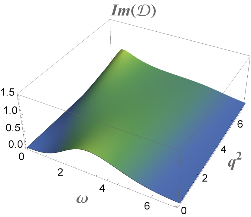
(b)

Figure 2: The $\omega$-, $q$-dependence of (a) $Re(\mathcal{D}(\omega,q^{2}))$, (b) $Im(\mathcal{D}(\omega,q^{2}))$.

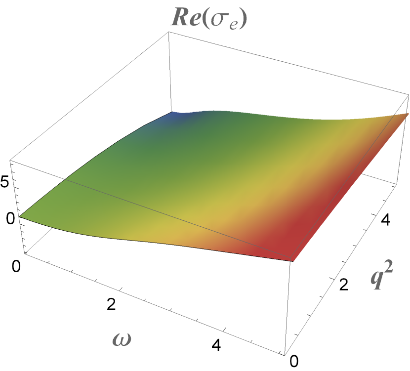
(a)

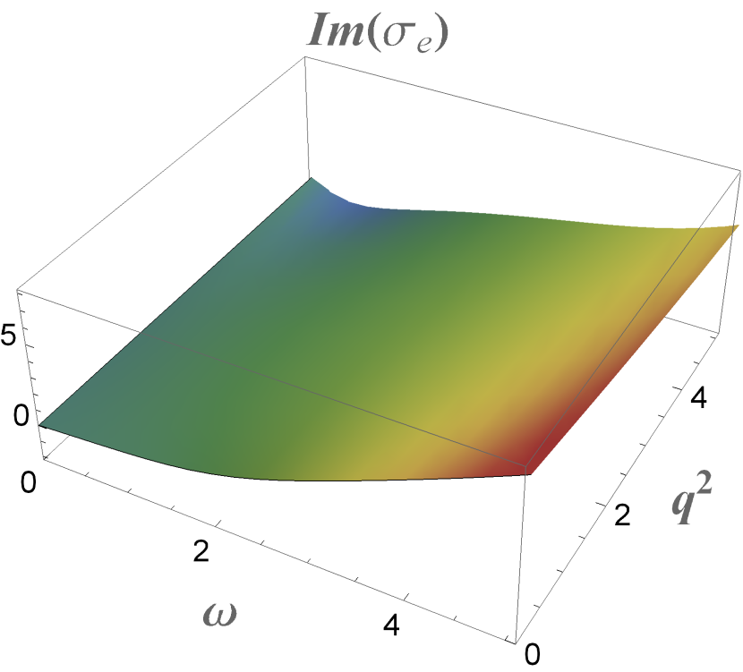
(b)

Figure 3: Ther $\omega$-, $q$-dependence of (a) $Re(\sigma_{e}(\omega,q^{2}))$, (b) $Im(\sigma_{e}(\omega,q^{2}))$.

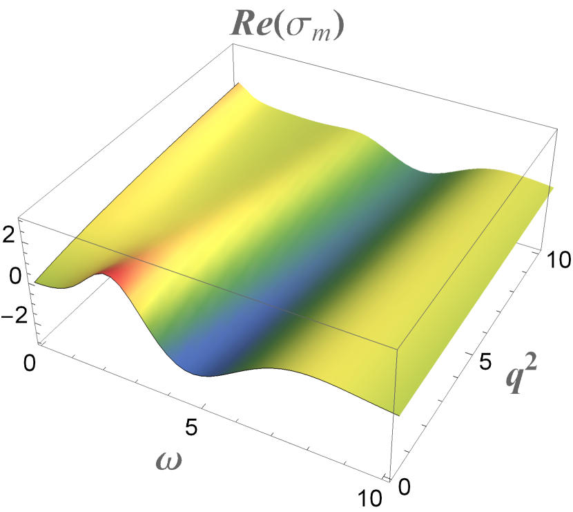
(a)

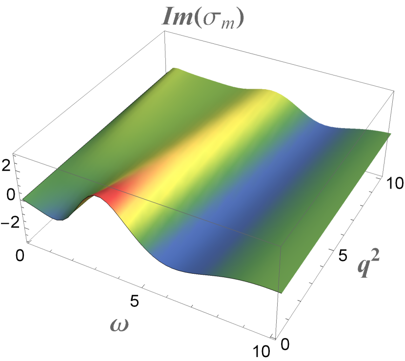
(b)

Figure 4: The $\omega$-, $q$-dependence of (a) $Re(\sigma_{m}(\omega,q^{2}))$, (b) $Im(\sigma_{m}(\omega,q^{2}))$.

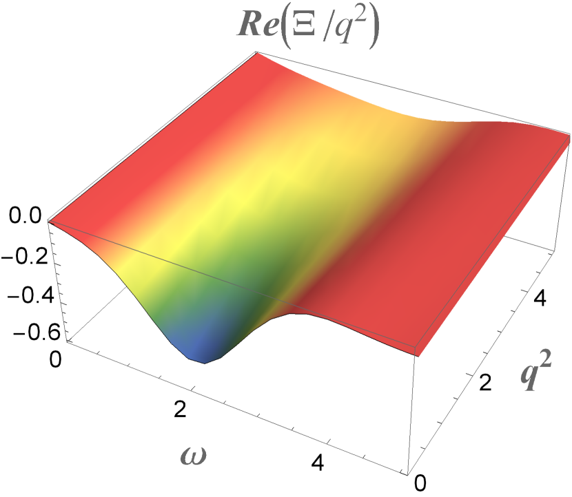
(a)

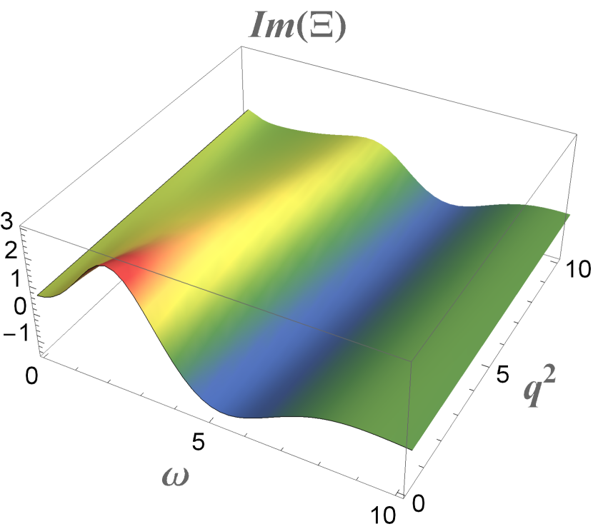
(b)

Figure 5: The $\omega$-, $q$-dependence of the coefficients (a) $Re(\Xi(\omega,q^{2}))$ (b) $Im(\Xi(\omega,q^{2}))$

The noise-noise correlator

Finally, the noise-noise correlator $-iG_{0}$ is displayed in Figure 6 as a function of $\omega$ and $q^{2}$. In Figure 7(a), we plot the same function, but as a 2d slices at fixed representative values of $q^{2}$. Since $-iG_{0}$ is proportional to $q^{2}$ up to sufficiently large momentum, we scale this dependence out in Figures 6 and 7(a). As is clear from the plots, $-iG_{0}$ initially oscillates as function of $\omega$ but quickly vanishes at large frequencies.

In order to better illustrate the coloured nature of the noise-noise correlator, we perform an inverse Fourier transform of $-iG_{0}$ with respect to the frequency, thus obtaining the time dependence of the correlator. The analysis is performed for fixed values of momentum $q$ and the results are displayed in Figure 7(b). It might be interesting to additionally perform the inverse Fourier transform in the spatial momentum, so to obtain the full space-time dependence of the correlator. Yet, this turns out to be numerically too expensive and we have decided not to pursue this analysis.

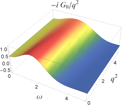
Figure 6: The $\omega$-, $q^{2}$-dependence of $-iG_{0}(\omega,q^{2})/q^{2}$

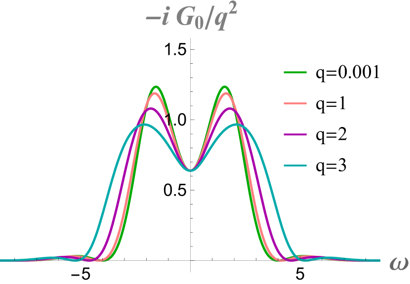
(a)

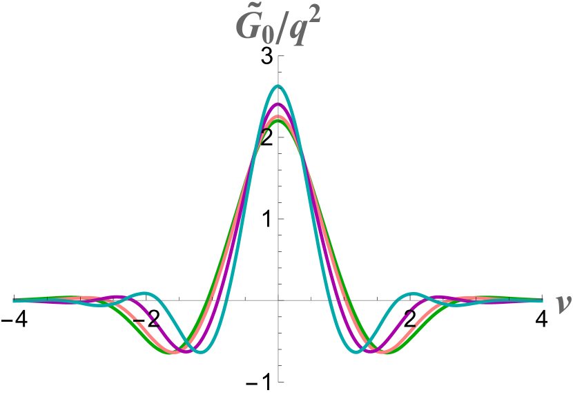
(b)

Figure 7: (a) The $\omega$-dependence of $-iG_{0}(\omega)/q^{2}$ at fixed $q$-slices; (b) The inverse Fourier transform of $-iG_{0}(\omega)/q^{2}$ at fixed $q$-slices.

6 Summary and Outlook

In this work we have further developed the off-shell SK holography. While the core element of the formalism is the geometry proposed in Glorioso:2018mmw , our approach to solving the bulk EOMs is different from that of Glorioso:2018mmw . When discussing the hydrodynamic expansion, one has to be very careful with the non-commutativity of the hydrodynamic limit vs the near horizon limit. Particularly, in order to reach a certain accuracy in the effective action, EOMs must be expanded to higher orders in the momenta. Our formalism completely avoids this subtlety since at no place it relies on the hydrodynamic expansion.

Starting from the off-shell SK holography, we have derived the effective action Crossley:2015evo for the charge diffusion and computed all order TCFs ($w_{1}...w_{9}$) parameterising it. These TCFs display various types of behaviour as functions of momenta, without any clear pattern. The evolution of $w_{1}...w_{9}$ from small momenta (the hydrodynamic limit) to very large momenta can be thought as a flow of the effective action from IR to UV. While we have not analysed it in any detail, the flow corresponds to integrating in of the heavy quasi-normal modes. It would be interesting to better understand this relation. Putting the effective action on-shell, we reproduced the prescription Son:2002sd for the retarded two-point current-current correlators.

The constitutive relation (3) for the current follows from the off-shell effective action. It is parameterised by four TCFs: the diffusion, electric conductivity, magnetic conductivity, and a thermal force. The latter is a new element emerging from the SK formalism. The thermal force is responsible for fluctuations/noise in the current. Due to linearity of the Maxwell’s theory in the bulk, the noise is Gaussian, though coloured (non-local in space-time). We have demonstrated that by explicitly performing the inverse Fourier transform of the noise-noise correlator to the real time.

Our new results for the diffusion TCF, electric and magnetic conductivities are different from the ones reported earlier in Bu:2015ame , even though they lead to identical two-point retarded correlators. The disagreement originates from different holographic dictionaries used to define the off-shell currents. As discussed in Appendix E, the off-shell formalism of Bu:2015ame defines the current entirely in terms of the normalisable modes, while from the SK holography we now learn that there appear additional terms contributing to the current.

The Maxwell’s theory in the bulk, even though much more complicated than a free scalar theory, provides a simple Gaussian theory on the boundary. A much more challenging problem would be to consider stochastic neutral flows, which amounts to embedding the fluid/gravity correspondence Kovtun:2004de ; Policastro:2001yc ; Policastro:2002se ; Policastro:2002tn ; Son:2002sd ; Bhattacharyya:2008jc (with dissipations only) into an EFT framework. This problem would require us to further develop the SK holography, particularly addressing the questions of non-Gaussian noise, dynamical horizon, etc.

Another very interesting direction would be to learn about hydrodynamic fluctuations associated with transport induced by chiral anomaly. While some relevant discussion could be found in Glorioso:2017lcn ; Haehl:2013hoa ; Iatrakis:2015fma ; Lin:2018nxj ; Liang:2020sgr , the topic remains largely unexplored. From the perspective of the SK holography, the problem could be addressed within the Maxwell-Chern-Simons theory in the bulk. Stochastic chiral hydrodynamics is expected to be rich with many new phenomena.

Appendix A The effective action from the basis decomposition

In this appendix we demonstrate how the effective action (2.1) is derived from (61). Following the formalism of Bu:2015ame , the bulk gauge fields $C_{\mu}$ can be linearly decomposed in terms of the basic tensor structures built from $B_{r\mu}$ and $B_{a\mu}$,

$$C_{v}=S_{1}B_{rv}+S_{2}\partial_{k}B_{rk}+S_{3}B_{av}+S_{4}\partial_{k}B_{ak},$$

$$C_{i}=V_{1}B_{ri}+V_{2}\partial_{i}B_{rv}+V_{3}\partial_{i}\partial_{k}B_{rk}+V_{4}B_{ai}+V_{5}\partial_{i}B_{av}+V_{6}\partial_{i}\partial_{k}B_{ak},$$ (158)

where the decomposition coefficients (bulk-to-boundary propagators) $S_{i},V_{i}$ are $SO(3)$ scalar functionals of the spacetime derivative operators $\partial_{\mu}$, and functions of the radial coordinate $r$:

$$S_{i}=S_{i}(r,\partial_{v},\vec{\partial}),\qquad V_{i}=V_{i}(r,\partial_{v},\vec{\partial}).$$ (159)

The boundary conditions for $S_{i},V_{i}$ are translated from those of $C_{\mu}$ :

$$r=\infty_{1}:\quad S_{1}=V_{1}=1,\quad S_{3}=V_{4}=\frac{1}{2},\qquad{\rm others}=0,$$

$$r=\infty_{2}:\quad S_{1}=V_{1}=1,\quad S_{3}=V_{4}=-\frac{1}{2},\quad\;{\rm others}=0.$$ (160)

In Fourier space, $(\partial_{v},\vec{\partial})\to(-i\omega,i\vec{q})$, these decomposition coefficients become functions of the momenta,

$$S_{i}(r,\partial_{v},\vec{\partial})\to S_{i}(r,\omega,q^{2}),\qquad V_{i}(r,\partial_{v},\vec{\partial})\to V_{i}(r,\omega,q^{2}).$$ (161)

With the help of (158) the original PDEs (43) reduce to a system of linear ODEs. Near $r=\infty_{1,2}$, the decomposition coefficients $S_{i},V_{i}$ can be expanded. Taking into account the boundary conditions (A), the expansion takes the form

$$S_{i}(r\to\infty_{1})=\cdots+\frac{s_{1i}}{r^{2}}+\cdots,\qquad S_{i}(r\to\infty_{2})=\cdots+\frac{s_{2i}}{r^{2}}+\cdots,$$

$$V_{i}(r\to\infty_{1})=\cdots+\frac{v_{1i}}{r^{2}}+\cdots,\qquad V_{i}(r\to\infty_{2})=\cdots+\frac{v_{2i}}{r^{2}}+\cdots.$$ (162)

where the coefficients $s_{1i},v_{1i}$ and $s_{2i},v_{2i}$ are respective normalizable modes.

Substituting the decomposition (158) into (61), the effective Lagrangian in the $(r,a)$-basis reads

$$\mathcal{L}_{\rm eff}= -B_{rv}s_{a1}B_{rv}-B_{rv}s_{a2}\partial_{k}B_{rk}+B_{rk}v_{a1}B_{rk}+B_{rk}v_{a2}\partial_{k}B_{rv}+B_{rk}v_{a3}\partial_{k}\partial_{l}B_{rl}$$

$$+(-B_{rv}s_{a3}B_{av}-B_{av}s_{r1}B_{rv})+(-B_{rv}s_{a4}\partial_{k}B_{ak}+B_{ak}v_{r2}\partial_{k}B_{rv})$$

$$+(-B_{av}s_{r2}\partial_{k}B_{rk}+B_{rk}v_{a5}\partial_{k}B_{av})-B_{av}s_{r3}B_{av}+(-B_{av}s_{r4}\partial_{k}B_{ak}+B_{ak}v_{r5}\partial_{k}B_{av})$$

$$+(B_{rk}v_{a4}B_{ak}+B_{ak}v_{r1}B_{rk})+(B_{rk}v_{a6}\partial_{k}\partial_{l}B_{al}+B_{ak}v_{r3}\partial_{k}\partial_{l}B_{rl})+B_{ak}v_{r4}B_{ak}$$

$$+B_{ak}v_{r6}\partial_{k}\partial_{l}B_{al}+\frac{1}{2}\partial_{k}B_{ak}\partial_{v}B_{rv}-\frac{1}{2}B_{av}\partial_{v}\partial_{k}B_{rk}+\frac{1}{2}B_{av}{\vec{\partial}}^{\,2}B_{rv}-\frac{1}{2}B_{ak}\partial_{v}^{2}B_{rk}$$

$$+\frac{1}{4}\mathcal{F}_{ajk}\mathcal{F}_{rjk}+B_{av}\partial_{v}^{2}B_{rv}.$$ (163)

Here, the coefficients are represented in the $(r,a)$-basis:

$$s_{ai}=s_{1i}-s_{2i},\qquad s_{ri}=\frac{1}{2}(s_{1i}+s_{2i}),\qquad i=1,2,3,4,$$

$$v_{ai}=v_{1i}-v_{2i},\qquad v_{ri}=\frac{1}{2}(v_{1i}+v_{2i}),\qquad i=1,2,\cdots,6.$$ (164)

The first line of (A) must vanish within the usual $(r,a)$ scheme. Indeed within the holographic representation of the SK contour:

$$s_{a1}=s_{a2}=v_{a1}=v_{a2}=v_{a3}=0.$$ (165)

To compare with Crossley:2015evo , (A) has to be rewritten so that all the $a$-fields are placed on the left, in all terms, say

$$\int d^{4}xB_{rv}(x)s_{a3}(\partial_{t},\vec{\partial})B_{av}(x)=\int d^{4}xB_{av}(x)s_{a3}(-\partial_{v},-\vec{\partial})B_{rv}(x).$$ (166)

Introducing $w_{i}=w_{i}(\partial_{v},\vec{\partial})$ as

$$\frac{i}{2}w_{1}(\partial_{v},\vec{\partial})=-s_{r3}(\partial_{v},\vec{\partial}),$$

$$\frac{i}{2}w_{2}(\partial_{v},\vec{\partial})=v_{r4}(\partial_{v},\vec{\partial}),$$

$$\frac{i}{2}w_{3}(\partial_{v},\vec{\partial})=-v_{r6}(\partial_{v},\vec{\partial}),$$

$$iw_{4}(\partial_{v},\vec{\partial})=-s_{r4}(\partial_{v},\vec{\partial})-v_{r5}(-\partial_{v},-\vec{\partial}),$$

$$w_{5}(\partial_{v},\vec{\partial})=\partial_{v}^{2}+\frac{1}{2}\vec{\partial}^{2}-s_{r1}(\partial_{v},\vec{\partial})-s_{a3}(-\partial_{v},-\vec{\partial})$$

$$w_{6}(\partial_{v},\vec{\partial})\partial_{v}=-\frac{1}{2}-s_{r2}(\partial_{v},\vec{\partial})-v_{a5}(-\partial_{v},-\vec{\partial}),$$

$$w_{7}(\partial_{v},\vec{\partial})=\frac{1}{2}\partial_{v}-s_{a4}(-\partial_{v},-\vec{\partial})-v_{r2}(\partial_{v},\vec{\partial})$$

$$w_{8}(\partial_{v},\vec{\partial})\partial_{v}=-\frac{1}{2}\partial_{v}^{2}+v_{a4}(-\partial_{v},-\vec{\partial})+v_{r1}(\partial_{v},\vec{\partial})+\left[v_{a6}(-\partial_{v},-\vec{\partial})+v_{r3}(\partial_{v},\vec{\partial})\right]{\vec{\partial}}^{2},$$

$$w_{9}(\partial_{v},\vec{\partial})=\frac{1}{2}+v_{a6}(-\partial_{v},-\vec{\partial})+v_{r3}(\partial_{v},\vec{\partial}),$$ (167)

the effective Lagrangian (A) is cast into (2.1), consistently with Crossley:2015evo .

Appendix B Validating (77)

In subsection 4.2, we derived the discontinuity relation (77). Our goal here is to verify this condition by computing both left-hand side (LHS) and right-hand side (RHS) of (77), starting from the solutions constructed in the subsections 4.3 and 4.4.

The RHS of (77) is proportional to $\nabla_{M}F^{Mr}$. Recall that in general, $\nabla_{M}F^{Mr}$ has a very simple dependence on $r$, see (46). In (46) the values of $\mathcal{C}^{\rm up}$ and $\mathcal{C}^{\rm dw}$ should be determined from the solutions established in subsections 4.3 and 4.4. As has been emphasised towards the end of subsection 4.3, among the four linearly independent solutions in the longitudinal sector, only the polynomial solution $\{C_{v}^{\rm pn},C_{x}^{\rm pn}\}$ does not automatically satisfy the constraint equation (69). Hence $\mathcal{C}^{\rm up,\,dw}$ must be proportional to the coefficients $n_{\parallel}^{\rm up,\,dw}$ multiplying the polynomial solutions. More precisely, by taking the near horizon limit of (46), we have

$$\mathcal{C}^{\rm up}(k)=i\omega r_{h}^{3}\tilde{C}_{t}^{{\rm pn}\,h}n_{\parallel}^{\rm up},\qquad\qquad\mathcal{C}^{\rm dw}(k)=i\omega r_{h}^{3}\tilde{C}_{t}^{{\rm pn}\,h}n_{\parallel}^{\rm dw}.$$ (168)

Thus the RHS of (77) reads

$$\lim_{\Delta\to 0}\int_{r_{-}-\Delta}^{r_{+}+\Delta}dr\frac{\nabla_{M}F^{Mr}}{f(r)} =\frac{\mathcal{C}^{\rm dw}(k)}{i\omega r_{h}^{3}}e^{i\omega\zeta_{1}(r_{h}-\epsilon)}-\frac{\mathcal{C}^{\rm up}(k)}{i\omega r_{h}^{3}}e^{i\omega\zeta_{2}(r_{h}-\epsilon)}$$

$$=\tilde{C}_{t}^{{\rm pn}\,h}\left[n_{\parallel}^{\rm dw}e^{i\omega\zeta_{1}(r_{h}-\epsilon)}-n_{\parallel}^{\rm up}e^{i\omega\zeta_{2}(r_{h}-\epsilon)}\right].$$ (169)

Based on the solutions found in 4.3 and 4.4, the discontinuity of $\partial_{r}C_{v}$ is

$$\partial_{r}C_{v}(r_{+})-\partial_{r}C_{v}(r_{-})= n_{\parallel}^{\rm up}\partial_{r}C_{v}^{\rm pn}\big{|}_{r=r_{+}}-n_{\parallel}^{\rm dw}\partial_{r}C_{v}^{\rm pn}\big{|}_{r=r_{-}}$$

$$= \frac{i\omega}{f(r)}n_{\parallel}^{\rm up}C_{v}^{\rm pn}(r)\bigg{|}_{r=r_{+}}-\frac{i\omega}{f(r)}n_{\parallel}^{\rm dw}C_{v}^{\rm pn}(r)\bigg{|}_{r=r_{-}}$$

$$+\tilde{C}_{t}^{{\rm pn}\,h}n_{\parallel}^{\rm up}e^{i\omega\zeta_{2}(r_{h}-\epsilon)}-\tilde{C}_{t}^{{\rm pn}\,h}n_{\parallel}^{\rm dw}e^{i\omega\zeta_{1}(r_{h}-\epsilon)}$$ (170)

While $C_{v}$ is continuous across the cutting slice, $C_{r}=-C_{v}/f(r)$ has a jump:

$$\frac{C_{v}(r)}{f(r)}\bigg{|}_{r=r_{+}}-\frac{C_{v}(r)}{f(r)}\bigg{|}_{r=r_{-}}=\frac{n_{\parallel}^{\rm up}}{f(r)}C_{v}^{\rm pn}(r)\bigg{|}_{r=r_{+}}-\frac{n_{\parallel}^{\rm dw}}{f(r)}C_{v}^{\rm pn}(r)\bigg{|}_{r=r_{-}}.$$ (171)

So, the LHS of (77) is computed as

$$F^{rv}(r_{+})-F^{rv}(r_{-}) =\left[\frac{i\omega}{f(r)}-\partial_{r}\right]C_{v}\bigg{|}_{r=r_{+}}-\left[\frac{i\omega}{f(r)}-\partial_{r}\right]C_{v}\bigg{|}_{r=r_{-}}$$

$$=\tilde{C}_{t}^{{\rm pn}\,h}n_{\parallel}^{\rm dw}e^{i\omega\zeta_{1}(r_{h}-\epsilon)}-\tilde{C}_{t}^{{\rm pn}\,h}n_{\parallel}^{\rm up}e^{i\omega\zeta_{2}(r_{h}-\epsilon)}$$ (172)

which is exactly the same as (169).

Appendix C Son-Starinets prescription for retarded correlators revisited

At the early days of the fluid-gravity correspondence, Son and Starinets Son:2002sd proposed a prescription for computing Minkowski-space retarded correlators. The prescription is formulated entirely within a single copy of the doubled BH-AdS, and does not rely on SK holography. Yet, a proper derivation of the prescription from the SK holography is missing, and in this appendix we provide one. While there have been earlier works in this direction, particularly Herzog:2002pc , which considered SK matrix propagator for a scalar field starting from an eternal black hole in AdS space Maldacena:2001kr , the SK geometry of Glorioso:2018mmw adopted here is different. Furthermore, we are not aware of any derivation for the $U(1)$ field available in the literature.

The prescription of Son:2002sd relates the retarded correlators to the ingoing solution in a single BH AdS. Starting from the SK holography, we can reproduce the result by taking a few alternative paths. First, the correlators could be obtained from the off-shell effective Lagrangian (2.1) by integrating out the dynamical fields $\varphi_{r}$ and $\varphi_{a}$ (8). The result is the boundary generating functional $W[\mathcal{A}_{a\mu},\mathcal{A}_{r\mu}]$ of the external fields only, form which the correlators could be read off straightforwardly. For the Lagrangian quadratic in the dynamical fields, like (2.1), integrating out $\varphi_{r}$ and $\varphi_{a}$ could be done by imposing their classical EOMs. On the bulk side, this corresponds to imposing the constraint equation. Putting the solutions (108) on-shell is equivalent to setting $n_{\parallel}^{\rm up}=n_{\parallel}^{\rm dw}=0$, which via (112) and (113) yields classical solutions for $\varphi_{r}$ and $\varphi_{a}$.

Alternatively, we could start with the constitutive relation (18), and use the continuity equation, which leads to the retarded current-current correlators expressed in terms of the TCFs Bu:2015ame :

$$G_{R}^{\perp\perp}=i\omega\sigma_{e}+q^{2}\sigma_{m},\qquad G_{R}^{vv}=\frac{q^{2}\sigma_{e}}{-i\omega+q^{2}\mathcal{D}},\qquad G_{R}^{vx}=\frac{\omega q\sigma_{e}}{-i\omega+q^{2}\mathcal{D}},$$

$$G_{R}^{xx}=\frac{\omega^{2}\sigma_{e}}{-i\omega+q^{2}\mathcal{D}}.$$ (173)

These expressions could be algebraically traced back to the ingoing solution in a single copy of BH-AdS.

Yet, we believe the most illuminating derivation is to reconsider the problem from the very beginning, starting within the on-shell SK holography, which offers a possibility to work directly with gauge invariant fields

$$E_{\perp}=\partial_{\perp}C_{v}-\partial_{v}C_{\perp},\qquad\qquad E_{x}=\partial_{x}C_{v}-\partial_{v}C_{x}.$$ (174)

EOMs for the bulk electric fields $E_{\perp}$ and $E_{x}$ are

$$\partial_{r}\left[rf(r)\partial_{r}E_{\perp}\right]-2i\omega r\partial_{r}E_{\perp}-i\omega E_{\perp}-q^{2}r^{-1}E_{\perp}=0,$$

$$\partial_{r}\left[\frac{rf(r)}{\omega^{2}-r^{-2}f(r)q^{2}}\partial_{r}E_{x}\right]-\frac{2i\omega r}{\omega^{2}-r^{-2}f(r)q^{2}}\partial_{r}E_{x}+\partial_{r}\left[\frac{-i\omega r}{\omega^{2}-r^{-2}f(r)q^{2}}\right]E_{x}$$

$$-\frac{r^{-1}q^{2}}{\omega^{2}-r^{-2}f(r)q^{2}}E_{x}=0.$$ (175)

In the equation for $E_{x}$, there is a singularity at $r=r_{h}(1-\omega^{2}/q^{2})^{-1/4}$ for space-like momenta, which is however integrable CaronHuot:2006te .

The on-shell bulk action (32) reads

$$S_{0}= -\frac{1}{2}\int\frac{d\omega dq}{(2\pi)^{2}}\left\{\frac{r}{i\omega}E_{\perp}(r,-k)E_{\perp}(r,k)+\frac{rf(r)}{\omega^{2}}E_{\perp}(r,-k)\partial_{r}E_{\perp}(r,k)\right.$$

$$\left.-\frac{i\omega r}{\omega^{2}-r^{-2}f(r)q^{2}}E_{x}(r,-k)E_{x}(r,k)+\frac{rf(r)}{\omega^{2}-r^{-2}f(r)q^{2}}E_{x}(r,-k)\partial_{r}E_{x}(r,k)\right\}\bigg{|}_{r=\infty_{1}}$$

$$+\frac{1}{2}\int\frac{d\omega dq}{(2\pi)^{2}}\left\{\frac{r}{i\omega}E_{\perp}(r,-k)E_{\perp}(r,k)+\frac{rf(r)}{\omega^{2}}E_{\perp}(r,-k)\partial_{r}E_{\perp}(r,k)\right.$$

$$\left.-\frac{i\omega r}{\omega^{2}-r^{-2}f(r)q^{2}}E_{x}(r,-k)E_{x}(r,k)+\frac{rf(r)}{\omega^{2}-r^{-2}f(r)q^{2}}E_{x}(r,-k)\partial_{r}E_{x}(r,k)\right\}\bigg{|}_{r=\infty_{2}}.$$ (176)

Near each AdS boundary, $r\to\infty_{s}$ with $s=(1,2)$, the bulk electric fields $E_{\perp}$ and $E_{x}$ behave as

$$E_{s,\perp}(r,k)\xrightarrow[]{r\to\infty_{s}}E_{s,\perp}^{(0)}(k)-\frac{i\omega}{r}E_{s,\perp}^{(0)}(k)+\frac{1}{2}(\omega^{2}-q^{2})E_{s,\perp}^{(0)}(k)\frac{\log r}{r^{2}}+\frac{E_{s,\perp}^{(2)}(k)}{r^{2}}+\cdots,$$

$$E_{s,x}(r,k)\xrightarrow[]{r\to\infty_{s}}E_{s,x}^{(0)}(k)-\frac{i\omega}{r}E_{s,x}^{(0)}(k)+\frac{1}{2}(\omega^{2}-q^{2})E_{s,x}^{(0)}(k)\frac{\log r}{r^{2}}+\frac{E_{s,x}^{(2)}(k)}{r^{2}}+\cdots.$$ (177)

Then, the generating functional of the boundary theory (i.e., the on-shell bulk action) becomes

$$W[\mathcal{A}_{a\mu},\mathcal{A}_{r\mu}]=S_{0}+S_{\rm c.t.}=\int\frac{d\omega dq}{(2\pi)^{2}}\mathcal{L}_{\rm eff}^{\rm os}[\mathcal{F}_{alv},\mathcal{F}_{rlv}],$$ (178)

where

$$\mathcal{L}_{\rm eff}^{\rm os}= \frac{1}{\omega^{2}}\left[\mathcal{F}_{a\perp v}(-k)E_{r\perp}^{(2)}(k)+\mathcal{F}_{r\perp v}(-k)E_{a\perp}^{(2)}(k)\right]$$

$$+\frac{1}{\omega^{2}-q^{2}}\left[\mathcal{F}_{axv}(-k)E_{rx}^{(2)}(k)+\mathcal{F}_{rxv}(-k)E_{ax}^{(2)}(k)\right]$$

$$+\frac{1}{2}\mathcal{F}_{a\perp v}(-k)\mathcal{F}_{r\perp v}(-k)+\frac{1}{2}\mathcal{F}_{ax\perp}(-k)\mathcal{F}_{rx\perp}(k)+\frac{\omega^{2}+q^{2}}{2(\omega^{2}-q^{2})}\mathcal{F}_{axv}(-k)\mathcal{F}_{rxv}(k).$$ (179)

The EOMs (175) are solved similarly to the transverse sector $C_{\perp}$ in Section 4. The piecewise solutions will be glued under matching conditions derived in subsection 4.2 (imposing the constraint equation $\nabla_{M}F^{Mr}=0$)

$$E_{i}(r_{+})=E_{i}(r_{-}),\qquad f(r_{h}-\epsilon)\left[\partial_{r}E_{i}(r_{+})-\partial_{r}E_{i}(r_{-})\right]=0,\qquad i=\perp,x.$$ (180)

Near the boundaries

$$E_{i}(r\to\infty_{1})=\mathcal{F}_{1iv},\qquad E_{i}(r\to\infty_{2})=\mathcal{F}_{2iv},\qquad i=\perp,x.$$ (181)

Over the entire contour of Figure 1, the solutions for $E_{\perp}$ and $E_{x}$ are

$$E_{\perp}^{\rm up}(r,\omega,q)=l_{\perp}E_{\perp}^{\rm ig}(r,\omega,q)+m_{\perp}E_{\perp}^{\rm ig}(r,-\omega,q)e^{2i\omega\zeta_{2}(r)},\qquad\qquad r\in[r_{h}-\epsilon,\infty_{2}),$$

$$E_{\perp}^{\rm dw}(r,\omega,q)=l_{\perp}E_{\perp}^{\rm ig}(r,\omega,q)+m_{\perp}e^{-\beta\omega}E_{\perp}^{\rm ig}(r,-\omega,q)e^{2i\omega\zeta_{1}(r)},\qquad r\in[r_{h}-\epsilon,\infty_{1}),$$ (182)

$$E_{x}^{\rm up}(r,\omega,q)=l_{x}E_{x}^{\rm ig}(r,\omega,q)+m_{x}E_{x}^{\rm ig}(r,-\omega,q)e^{2i\omega\zeta_{2}(r)},\qquad\qquad r\in[r_{h}-\epsilon,\infty_{2}),$$

$$E_{x}^{\rm dw}(r,\omega,q)=l_{x}E_{x}^{\rm ig}(r,\omega,q)+m_{x}e^{-\beta\omega}E_{x}^{\rm ig}(r,-\omega,q)e^{2i\omega\zeta_{1}(r)},\qquad r\in[r_{h}-\epsilon,\infty_{1}),$$ (183)

where the superposition coefficients $l_{\perp}$, $m_{\perp}$, $l_{x}$ and $m_{x}$ are

$$l_{\perp}=\frac{\mathcal{F}_{r\perp v}(k)}{E_{\perp}^{\rm ig(0)}(k)}+\frac{1}{2}\coth\frac{\beta\omega}{2}\frac{\mathcal{F}_{a\perp v}(k)}{E_{\perp}^{\rm ig(0)}(k)},\qquad m_{\perp}=-\frac{\mathcal{F}_{a\perp v}(k)}{(1-e^{-\beta\omega})E_{\perp}^{\rm ig(0)}(\bar{k})},$$

$$l_{x}=\frac{\mathcal{F}_{rxv}(k)}{E_{x}^{\rm ig(0)}(k)}+\frac{1}{2}\coth\frac{\beta\omega}{2}\frac{\mathcal{F}_{axv}(k)}{E_{x}^{\rm ig(0)}(k)},\qquad m_{x}=-\frac{\mathcal{F}_{axv}(k)}{(1-e^{-\beta\omega})E_{x}^{\rm ig(0)}(\bar{k})}.$$ (184)

The near-boundary expansion of the ingoing solutions is

$$E_{\perp}^{\rm ig}(r,k)\xrightarrow[]{r\to\infty} E_{\perp}^{\rm ig(0)}(k)-\frac{i\omega E_{\perp}^{\rm ig(0)}(k)}{r}+\frac{1}{2}(\omega^{2}-q^{2})E_{\perp}^{\rm ig(0)}(k)\frac{\log r}{r}+\frac{E_{\perp}^{\rm ig(2)}(k)}{r^{2}}+\cdots,$$

$$E_{x}^{\rm ig}(r,k)\xrightarrow[]{r\to\infty} E_{x}^{\rm ig(0)}(k)-\frac{i\omega E_{x}^{\rm ig(0)}(k)}{r}+\frac{1}{2}(\omega^{2}-q^{2})E_{x}^{\rm ig(0)}(k)\frac{\log r}{r}+\frac{E_{x}^{\rm ig(2)}(k)}{r^{2}}+\cdots.$$ (185)

Substituting the superposition coefficients and representing the result in the $(r,a)$-basis, the field’s normalisable modes are

$$E_{a\perp}^{(2)}(k)= \frac{E_{\perp}^{\rm ig(2)}(\bar{k})}{E_{\perp}^{\rm ig(0)}(\bar{k})}\mathcal{F}_{a\perp v}(k),$$

$$E_{r\perp}^{(2)}(k)= \frac{1}{2}\coth\frac{\beta\omega}{2}\left[\frac{E_{\perp}^{\rm ig(2)}(k)}{E_{\perp}^{\rm ig(0)}(k)}-\frac{E_{\perp}^{\rm ig(2)}(\bar{k})}{E_{\perp}^{\rm ig(0)}(\bar{k})}\right]\mathcal{F}_{a\perp v}(k)+\frac{E_{\perp}^{\rm ig(2)}(k)}{E_{\perp}^{\rm ig(0)}(k)}\mathcal{F}_{r\perp v}(k),$$

$$E_{ax}^{(2)}(k)= \frac{E_{x}^{\rm ig(2)}(\bar{k})}{E_{x}^{\rm ig(0)}(\bar{k})}\mathcal{F}_{axv}(k),$$

$$E_{rx}^{(2)}(k)= \frac{1}{2}\coth\frac{\beta\omega}{2}\left[\frac{E_{x}^{\rm ig(2)}(k)}{E_{x}^{\rm ig(0)}(k)}-\frac{E_{x}^{\rm ig(2)}(\bar{k})}{E_{x}^{\rm ig(0)}(\bar{k})}\right]\mathcal{F}_{axv}(k)+\frac{E_{x}^{\rm ig(2)}(k)}{E_{x}^{\rm ig(0)}(k)}\mathcal{F}_{rxv}(k).$$ (186)

Finally, (179) reads

$$\mathcal{L}_{\rm eff}^{\rm os}= \frac{1}{\omega^{2}}\mathcal{F}_{a\perp v}(-k)\frac{1}{2}\coth\frac{\beta\omega}{2}\left[\frac{E_{\perp}^{\rm ig(2)}(k)}{E_{\perp}^{\rm ig(0)}(k)}-\frac{E_{\perp}^{\rm ig(2)}(\bar{k})}{E_{\perp}^{\rm ig(0)}(\bar{k})}\right]\mathcal{F}_{a\perp v}(k)$$

$$+\frac{1}{\omega^{2}}\mathcal{F}_{a\perp v}(-k)\left[\frac{2E_{\perp}^{\rm ig(2)}(k)}{E_{\perp}^{\rm ig(0)}(k)}+\frac{1}{2}\omega^{2}+\frac{1}{2}q^{2}\right]\mathcal{F}_{r\perp v}(k)$$

$$+\frac{1}{\omega^{2}-q^{2}}\mathcal{F}_{axv}(-k)\frac{1}{2}\coth\frac{\beta\omega}{2}\left[\frac{E_{x}^{\rm ig(2)}(k)}{E_{x}^{\rm ig(0)}(k)}-\frac{E_{x}^{\rm ig(2)}(\bar{k})}{E_{x}^{\rm ig(0)}(\bar{k})}\right]\mathcal{F}_{axv}(k)$$

$$+\frac{1}{\omega^{2}-q^{2}}\mathcal{F}_{axv}(-k)\left[\frac{2E_{x}^{\rm ig(2)}(k)}{E_{x}^{\rm ig(0)}(k)}+\frac{1}{2}\omega^{2}+\frac{1}{2}q^{2}\right]\mathcal{F}_{rxv}(k).$$ (187)

From the generating functional $W$, it is straightforward to read off all two-point correlation functions:

$$G_{R}^{\perp\perp}=\Pi^{T}(k),\qquad\qquad G_{S}^{\perp\perp}=G^{T}(k),$$

$$G_{R}^{vv}=\frac{q^{2}}{\omega^{2}-q^{2}}\Pi^{L}(k),\quad G_{R}^{vx}=\frac{\omega q}{\omega^{2}-q^{2}}\Pi^{L}(k),\quad G_{R}^{xx}=\frac{\omega^{2}}{\omega^{2}-q^{2}}\Pi^{L}(k),$$

$$G_{S}^{vv}=\frac{q^{2}}{\omega^{2}-q^{2}}G^{L}(k),\quad G_{S}^{vx}=\frac{\omega q}{\omega^{2}-q^{2}}G^{L}(k),\quad G_{S}^{xx}=\frac{\omega^{2}}{\omega^{2}-q^{2}}G^{L}(k),$$ (188)

where

$$\Pi^{T}(k)=\frac{2E_{\perp}^{\rm ig(2)}(k)}{E_{\perp}^{\rm ig(0)}(k)}+\frac{1}{2}\omega^{2}+\frac{1}{2}q^{2},\quad\Pi^{L}(\omega,q)=\frac{2E_{x}^{\rm ig(2)}(k)}{E_{x}^{\rm ig(0)}(k)}+\frac{1}{2}\omega^{2}+\frac{1}{2}q^{2},$$

$$G^{T}(k)=\frac{1}{2}\coth\frac{\beta\omega}{2}\left[\frac{E_{\perp}^{\rm ig(2)}(k)}{E_{\perp}^{\rm ig(0)}(k)}-\frac{E_{\perp}^{\rm ig(2)}(\bar{k})}{E_{\perp}^{\rm ig(0)}(\bar{k})}\right],$$

$$G^{L}(k)=\frac{1}{2}\coth\frac{\beta\omega}{2}\left[\frac{E_{x}^{\rm ig(2)}(k)}{E_{x}^{\rm ig(0)}(k)}-\frac{E_{x}^{\rm ig(2)}(\bar{k})}{E_{x}^{\rm ig(0)}(\bar{k})}\right].$$ (189)

From the EOMs (175), it is clear that $E_{\perp},E_{x}$ are functions of $q^{2}$. So, (189) satisfy the FDRs:

$$G^{T}(\omega,q)=\frac{1}{2}\coth\frac{\beta\omega}{2}{\rm Im}\left[\Pi^{T}(\omega,q)\right],\qquad G^{L}(\omega,q)=\frac{1}{2}\coth\frac{\beta\omega}{2}{\rm Im}\left[\Pi^{L}(\omega,q)\right].$$ (190)

We have reproduced the prescription of Son:2002sd for the retarded correlators. A couple of comments are in order. The above derivations have not imposed any KMS-type conditions, rather they follow from the SK holography. The original prescription of Son:2002sd correctly but a-priori unjustifiably ignores the horizon contribution to the on-shell action. From our derivation it is clear that only two AdS boundaries contribute to the boundary generating functional.

Appendix D Numerical results for $w_{5},w_{7},w_{8},w_{9}$

The results for $\omega$-, $q$-dependence of the coefficients $w_{5}$, $w_{7}$, $w_{8}$ and $w_{9}$ are displayed as 3D plots in Figures 8, 9, 10, 11 respectively. There is no clear universal pattern in the functional dependencies of these TCFs. They display different asymptotic behaviours at large momenta. For example, imaginary part of $w_{5}$ develops a growing ridge-like structure in the $\omega\simeq q$ region; imaginary parts of both $w_{7}$ and $w_{8}$ display a decreasing ridge-like behaviour also in the vicinity of $\omega\simeq q$ domain. For larger values of frequency (not shown in the plots), the amplitudes of all the TCFs ($w_{5},w_{7},w_{8},w_{9}$) seem to keep on growing. Each individual coefficient $w_{i}$ does not seem to have a clear physical interpretation and this is the reason in the main part of the text we rather focus on the diffusion TCF $\mathcal{D}$ and conductivities $\sigma_{e}$ and $\sigma_{m}$ only.

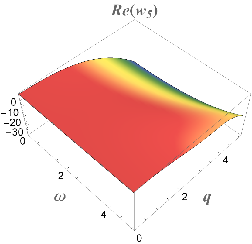
(a)

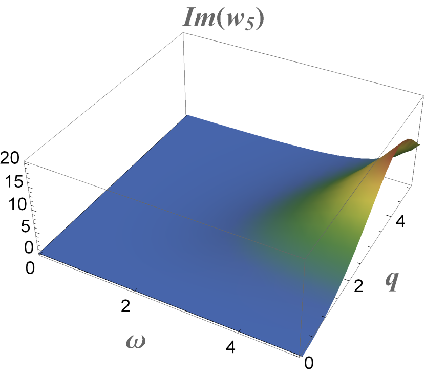
(b)

Figure 8: Plots for $\omega$-, $q$-dependence of the coefficients (a) $Re(w_{5}(\omega,q))$, (b) $Im(w_{5}(\omega,q))$.

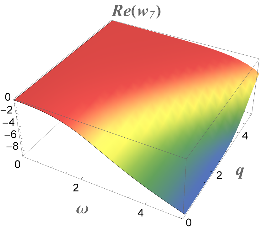
(a)

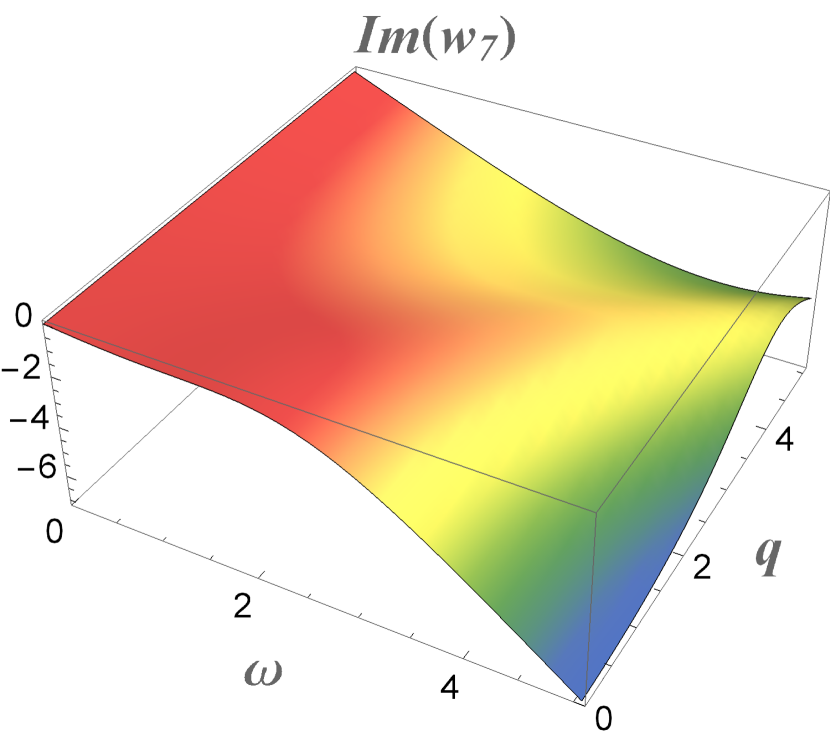
(b)

Figure 9: Plots for $\omega$-, $q$-dependence of the coefficients (a) $Re(w_{7}(\omega,q))$, (b) $Im(w_{7}(\omega,q))$.

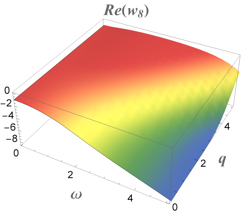
(a)

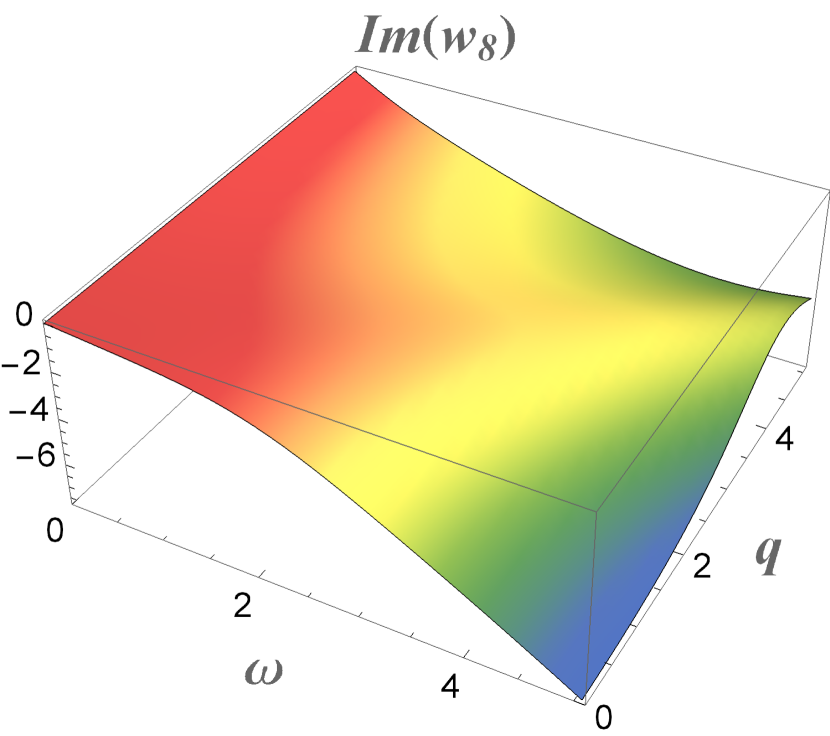
(b)

Figure 10: Plots for $\omega$-, $q$-dependence of the coefficients (a) $Re(w_{8}(\omega,q))$, (b) $Im(w_{8}(\omega,q))$.

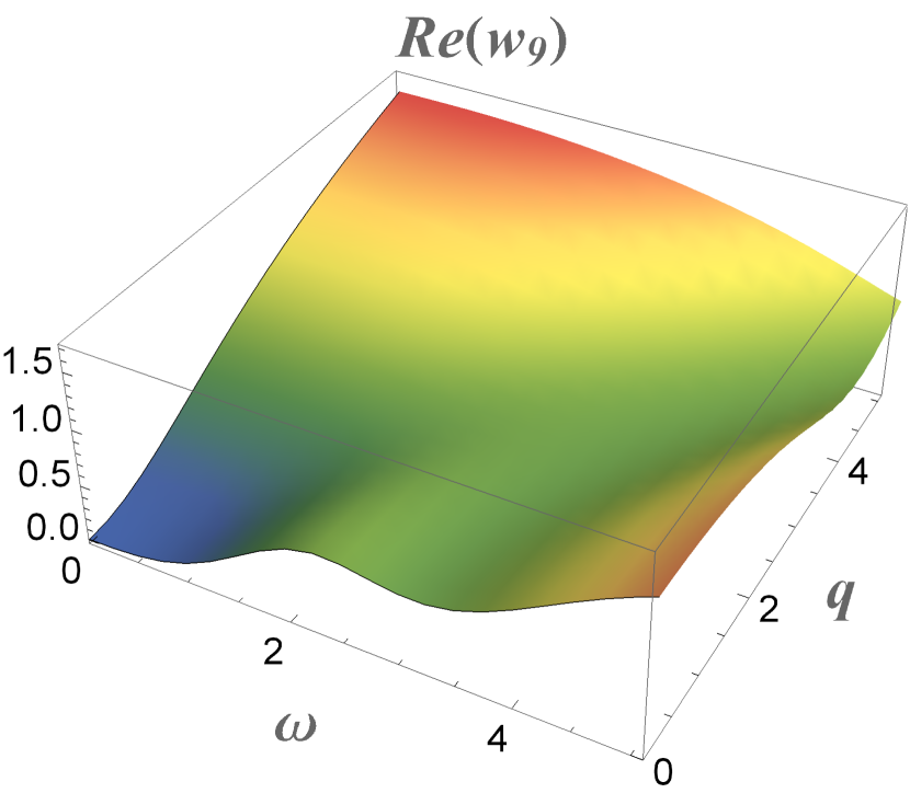
(a)

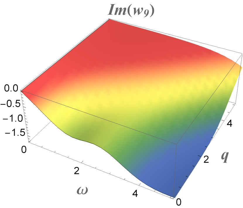
(b)

Figure 11: Plots for $\omega$-, $q$-dependence of the coefficients (a) $Re(w_{9}(\omega,q))$, (b) $Im(w_{9}(\omega,q))$.

It is important to notice that some of the TCFs $w_{i}$ vanish in the hydro limit. Yet, all of the TCFs are non-zero at finite momenta and contribute non-trivially to the effective action. In a sense this constitutes an evolution of the effective action from IR (hydro regime) to UV (all order/large momenta regime).

Appendix E Clarifying the origin of the discrepancy with Bu:2015ame

As discussed in the main text, our present results for the TCFs $\mathcal{D}$, $\sigma_{e}$ and $\sigma_{m}$ differ from the ones obtained previously in Bu:2015ame . In this Appendix, we identify the origin of this discrepancy.

The analysis of Bu:2015ame is carried in a single Schwarzschild-AdS₅. Instead of gluing the bulk solutions at the horizon implemented in the SK holography, regularity condition on the bulk fields was imposed in Bu:2015ame . This is equivalent to setting all the $a$-type fields, $B_{a\mu}$, to zero from the very start, at the level of equations of motion, thus making two segments of the SK contour identical. This immediately implies that an analog of the effective action along the SK contour vanishes, and, obviously, there is no possibility to vary it with respect to $B_{a\mu}$. Hence, the off shell formalism of Bu:2015ame is not embeddable into the fundamental framework based on SK non-equilibrium field theory.

Next, we are going to explicitly demonstrate how setting $B_{a\mu}=0$ at the very beginning leads to different constitutive relations compared to the ones of the present paper, when $B_{a\mu}=0$ is imposed at the very end of the calculation.

The horizon regularity condition is equivalent to having no outgoing mode. That is $h_{\perp}=h_{||}=0$. Hence, as mentioned, $B_{a\mu}=0$ and under this condition the bulk solutions of the present work are essentially identical to those of Bu:2015ame . Following the prescription of Son:2002sd , the hydrodynamic current in Bu:2015ame was identified with the normalisable modes of $C_{\mu}$. That is, using present language,

$$J_{v}^{\rm BLS}=2C_{rv}^{(2)}(k)|_{B_{a\mu}=0}+\cdots,\qquad J_{i}^{\rm BLS}=2C_{ri}^{(2)}(k)|_{B_{a\mu}=0}+\cdots,\qquad i=\perp,x,$$ (191)

where $\cdots$ stand for contact terms, the last six terms of (61). This current is to be compared with the hydrodynamical current $J_{hydro}$ introduced in (17).

In the transverse sector the two currents are equal, $J^{\perp}_{hydro}=J_{\perp}^{\rm BLS}$. Indeed, the current $J^{\perp}_{hydro}$ derived from the effective Lagrangian (120) is

$$J^{\perp}_{hydro}=\frac{2C_{\perp}^{\rm ig(2)}(k)}{C_{\perp}^{\rm ig(0)}(k)}B_{r\perp}(k)+\cdots,$$ (192)

which is exactly $2C_{r\perp}^{(2)}(k)|_{B_{a\mu}=0}$, cf. (118). The agreement within the transverse sector is related to the fact that the transverse current satisfies the continuity equation automatically, in this sense it is always on-shell.

The disagreement is entirely within the longitudinal sector and within the off-shell formalism only. On-shell, the results agree From the effective Lagrangian (128), the hydrodynamic current is

$$J^{v}_{hydro} =C_{rv}^{(2)}|_{B_{a\mu}=0}+\left[B_{rv}\frac{\delta C_{av}^{(2)}}{\delta B_{av}}-B_{rx}\frac{\delta C_{ax}^{(2)}}{\delta B_{av}}\right]+\cdots,$$

$$J^{x}_{hydro} =C_{rx}^{(2)}|_{B_{a\mu}=0}+\left[B_{rx}\frac{\delta C_{ax}^{(2)}}{\delta B_{ax}}-B_{rv}\frac{\delta C_{av}^{(2)}}{\delta B_{ax}}\right]+\cdots$$ (193)

Once the explicit expressions (124) and (126) are used, it is possible to demonstrate that $J^{||}_{hydro}\neq J_{||}^{\rm BLS}$ with the difference being proportional to $n=n^{\rm{up}}_{||}=n^{\rm{dw}}_{||}$m ($n^{\rm{up}}_{||}=n^{\rm{dw}}_{||}$ when $B_{a\mu}=0$ ). On-shell, $n=0$, and the results agree and lead to the very same current-current correlators discussed in the previous Appendix.

References

- (1) Y. Bu, M. Lublinsky, and A. Sharon, “ current from the AdS/CFT: diffusion, conductivity and causality,” JHEP 04 (2016) 136, arXiv:1511.08789 [hep-th].
- (2) L. Landau and E. Lifshitz, Fluid Mechanics. No. v. 6. Elsevier Science, 2013.
- (3) D. Forster, Hydrodynamic fluctuations, broken symmetry, and correlation functions. CRC Press, 1975.
- (4) L. P. Kadanoff and P. C. Martin, “Hydrodynamic equations and correlation functions,” Annals of Physics 24 (Oct., 1963) 419–469.
- (5) M. Lublinsky and E. Shuryak, “Improved Hydrodynamics from the AdS/CFT,” Phys. Rev. D 80 (2009) 065026, arXiv:0905.4069 [hep-ph].
- (6) Y. Bu and M. Lublinsky, “Linearly resummed hydrodynamics in a weakly curved spacetime,” JHEP 04 (2015) 136, arXiv:1502.08044 [hep-th].
- (7) J. M. Maldacena, “The Large N limit of superconformal field theories and supergravity,” Int. J. Theor. Phys. 38 (1999) 1113–1133, arXiv:hep-th/9711200.
- (8) S. Gubser, I. R. Klebanov, and A. M. Polyakov, “Gauge theory correlators from noncritical string theory,” Phys. Lett. B 428 (1998) 105–114, arXiv:hep-th/9802109.
- (9) E. Witten, “Anti-de Sitter space and holography,” Adv. Theor. Math. Phys. 2 (1998) 253–291, arXiv:hep-th/9802150.
- (10) P. Kovtun, D. T. Son, and A. O. Starinets, “Viscosity in strongly interacting quantum field theories from black hole physics,” Phys. Rev. Lett. 94 (2005) 111601, arXiv:hep-th/0405231.
- (11) G. Policastro, D. T. Son, and A. O. Starinets, “The Shear viscosity of strongly coupled N=4 supersymmetric Yang-Mills plasma,” Phys. Rev. Lett. 87 (2001) 081601, arXiv:hep-th/0104066.
- (12) G. Policastro, D. T. Son, and A. O. Starinets, “From AdS / CFT correspondence to hydrodynamics,” JHEP 09 (2002) 043, arXiv:hep-th/0205052.
- (13) G. Policastro, D. T. Son, and A. O. Starinets, “From AdS / CFT correspondence to hydrodynamics. 2. Sound waves,” JHEP 12 (2002) 054, arXiv:hep-th/0210220.
- (14) D. T. Son and A. O. Starinets, “Minkowski space correlators in AdS / CFT correspondence: Recipe and applications,” JHEP 09 (2002) 042, arXiv:hep-th/0205051 [hep-th].
- (15) S. Bhattacharyya, V. E. Hubeny, S. Minwalla, and M. Rangamani, “Nonlinear Fluid Dynamics from Gravity,” JHEP 02 (2008) 045, arXiv:0712.2456 [hep-th].
- (16) D. T. Son and A. O. Starinets, “Viscosity, Black Holes, and Quantum Field Theory,” Ann. Rev. Nucl. Part. Sci. 57 (2007) 95–118, arXiv:0704.0240 [hep-th].
- (17) Y. Bu and M. Lublinsky, “All order linearized hydrodynamics from fluid-gravity correspondence,” Phys. Rev. D 90 no. 8, (2014) 086003, arXiv:1406.7222 [hep-th].
- (18) Y. Bu and M. Lublinsky, “Linearized fluid/gravity correspondence: from shear viscosity to all order hydrodynamics,” JHEP 11 (2014) 064, arXiv:1409.3095 [hep-th].
- (19) S. Dubovsky, L. Hui, A. Nicolis, and D. T. Son, “Effective field theory for hydrodynamics: thermodynamics, and the derivative expansion,” Phys. Rev. D85 (2012) 085029, arXiv:1107.0731 [hep-th].
- (20) S. Dubovsky, L. Hui, and A. Nicolis, “Effective field theory for hydrodynamics: Wess-Zumino term and anomalies in two spacetime dimensions,” Phys. Rev. D89 no. 4, (2014) 045016, arXiv:1107.0732 [hep-th].
- (21) S. Endlich, A. Nicolis, R. A. Porto, and J. Wang, “Dissipation in the effective field theory for hydrodynamics: First order effects,” Phys. Rev. D88 (2013) 105001, arXiv:1211.6461 [hep-th].
- (22) S. Grozdanov and J. Polonyi, “Viscosity and dissipative hydrodynamics from effective field theory,” Phys. Rev. D 91 no. 10, (2015) 105031, arXiv:1305.3670 [hep-th].
- (23) A. Nicolis, R. Penco, and R. A. Rosen, “Relativistic Fluids, Superfluids, Solids and Supersolids from a Coset Construction,” Phys. Rev. D89 no. 4, (2014) 045002, arXiv:1307.0517 [hep-th].
- (24) P. Kovtun, G. D. Moore, and P. Romatschke, “Towards an effective action for relativistic dissipative hydrodynamics,” JHEP 07 (2014) 123, arXiv:1405.3967 [hep-ph].
- (25) M. Harder, P. Kovtun, and A. Ritz, “On thermal fluctuations and the generating functional in relativistic hydrodynamics,” JHEP 07 (2015) 025, arXiv:1502.03076 [hep-th].
- (26) F. M. Haehl, R. Loganayagam, and M. Rangamani, “The Fluid Manifesto: Emergent symmetries, hydrodynamics, and black holes,” JHEP 01 (2016) 184, arXiv:1510.02494 [hep-th].
- (27) F. M. Haehl, R. Loganayagam, and M. Rangamani, “Topological sigma models & dissipative hydrodynamics,” JHEP 04 (2016) 039, arXiv:1511.07809 [hep-th].
- (28) M. Crossley, P. Glorioso, and H. Liu, “Effective field theory of dissipative fluids,” JHEP 09 (2017) 095, arXiv:1511.03646 [hep-th].
- (29) M. Crossley, P. Glorioso, H. Liu, and Y. Wang, “Off-shell hydrodynamics from holography,” JHEP 02 (2016) 124, arXiv:1504.07611 [hep-th].
- (30) J. de Boer, M. P. Heller, and N. Pinzani-Fokeeva, “Effective actions for relativistic fluids from holography,” JHEP 08 (2015) 086, arXiv:1504.07616 [hep-th].
- (31) P. Glorioso and H. Liu, “The second law of thermodynamics from symmetry and unitarity,” arXiv:1612.07705 [hep-th].
- (32) P. Glorioso, M. Crossley, and H. Liu, “Effective field theory of dissipative fluids (II): classical limit, dynamical KMS symmetry and entropy current,” JHEP 09 (2017) 096, arXiv:1701.07817 [hep-th].
- (33) P. Glorioso, H. Liu, and S. Rajagopal, “Global Anomalies, Discrete Symmetries, and Hydrodynamic Effective Actions,” JHEP 01 (2019) 043, arXiv:1710.03768 [hep-th].
- (34) K. Jensen, N. Pinzani-Fokeeva, and A. Yarom, “Dissipative hydrodynamics in superspace,” JHEP 09 (2018) 127, arXiv:1701.07436 [hep-th].
- (35) F. M. Haehl, R. Loganayagam, and M. Rangamani, “Effective Action for Relativistic Hydrodynamics: Fluctuations, Dissipation, and Entropy Inflow,” JHEP 10 (2018) 194, arXiv:1803.11155 [hep-th].
- (36) K. Jensen, R. Marjieh, N. Pinzani-Fokeeva, and A. Yarom, “A panoply of Schwinger-Keldysh transport,” SciPost Phys. 5 no. 5, (2018) 053, arXiv:1804.04654 [hep-th].
- (37) P. Kovtun and L. G. Yaffe, “Hydrodynamic fluctuations, long time tails, and supersymmetry,” Phys. Rev. D68 (2003) 025007, arXiv:hep-th/0303010 [hep-th].
- (38) P. Kovtun, G. D. Moore, and P. Romatschke, “The stickiness of sound: An absolute lower limit on viscosity and the breakdown of second order relativistic hydrodynamics,” Phys. Rev. D84 (2011) 025006, arXiv:1104.1586 [hep-ph].
- (39) C. Young, J. I. Kapusta, C. Gale, S. Jeon, and B. Schenke, “Thermally Fluctuating Second-Order Viscous Hydrodynamics and Heavy-Ion Collisions,” Phys. Rev. C91 no. 4, (2015) 044901, arXiv:1407.1077 [nucl-th].
- (40) Y. Akamatsu, A. Mazeliauskas, and D. Teaney, “A kinetic regime of hydrodynamic fluctuations and long time tails for a Bjorken expansion,” Phys. Rev. C95 no. 1, (2017) 014909, arXiv:1606.07742 [nucl-th].
- (41) X. Chen-Lin, L. V. Delacretaz, and S. A. Hartnoll, “Theory of diffusive fluctuations,” Phys. Rev. Lett. 122 no. 9, (2019) 091602, arXiv:1811.12540 [hep-th].
- (42) A. Jain and P. Kovtun, “Non-universality of hydrodynamics,” arXiv:2009.01356 [hep-th].
- (43) M. Bluhm et al., “Dynamics of critical fluctuations: Theory — phenomenology — heavy-ion collisions,” Nucl. Phys. A1003 (2020) 122016, arXiv:2001.08831 [nucl-th].
- (44) A. Jain, P. Kovtun, A. Ritz, and A. Shukla, “Hydrodynamic effective field theory and the analyticity of hydrostatic correlators,” arXiv:2011.03691 [hep-th].
- (45) P. Kovtun, “Lectures on hydrodynamic fluctuations in relativistic theories,” J. Phys. A45 (2012) 473001, arXiv:1205.5040 [hep-th].
- (46) M. A. Stephanov, “Non-Gaussian fluctuations near the QCD critical point,” Phys. Rev. Lett. 102 (2009) 032301, arXiv:0809.3450 [hep-ph].
- (47) J. I. Kapusta and C. Young, “Causal Baryon Diffusion and Colored Noise,” Phys. Rev. C90 no. 4, (2014) 044902, arXiv:1404.4894 [nucl-th].
- (48) K.-c. Chou, Z.-b. Su, B.-l. Hao, and L. Yu, “Equilibrium and Nonequilibrium Formalisms Made Unified,” Phys. Rept. 118 (1985) 1–131.
- (49) A. Kamenev, Field Theory of Non-Equilibrium Systems. Cambridge University Press, 2011.
- (50) E. A. Calzetta and B.-L. B. Hu, Nonequilibrium Quantum Field Theory. Cambridge University Press, 2009.
- (51) C. Herzog and D. Son, “Schwinger-Keldysh propagators from AdS/CFT correspondence,” JHEP 03 (2003) 046, arXiv:hep-th/0212072.
- (52) K. Skenderis and B. C. van Rees, “Real-time gauge/gravity duality: Prescription, Renormalization and Examples,” JHEP 05 (2009) 085, arXiv:0812.2909 [hep-th].
- (53) K. Skenderis and B. C. van Rees, “Real-time gauge/gravity duality,” Phys. Rev. Lett. 101 (2008) 081601, arXiv:0805.0150 [hep-th].
- (54) E. Barnes, D. Vaman, C. Wu, and P. Arnold, “Real-time finite-temperature correlators from AdS/CFT,” Phys. Rev. D82 (2010) 025019, arXiv:1004.1179 [hep-th].
- (55) D. Nickel and D. T. Son, “Deconstructing holographic liquids,” New J. Phys. 13 (2011) 075010, arXiv:1009.3094 [hep-th].
- (56) D. T. Son and D. Teaney, “Thermal Noise and Stochastic Strings in AdS/CFT,” JHEP 07 (2009) 021, arXiv:0901.2338 [hep-th].
- (57) J. de Boer, V. E. Hubeny, M. Rangamani, and M. Shigemori, “Brownian motion in AdS/CFT,” JHEP 07 (2009) 094, arXiv:0812.5112 [hep-th].
- (58) J. Sonner and A. G. Green, “Hawking Radiation and Non-equilibrium Quantum Critical Current Noise,” Phys. Rev. Lett. 109 (2012) 091601, arXiv:1203.4908 [cond-mat.str-el].
- (59) J. de Boer, M. P. Heller, and N. Pinzani-Fokeeva, “Holographic Schwinger-Keldysh effective field theories,” JHEP 05 (2019) 188, arXiv:1812.06093 [hep-th].
- (60) P. Glorioso, M. Crossley, and H. Liu, “A prescription for holographic Schwinger-Keldysh contour in non-equilibrium systems,” arXiv:1812.08785 [hep-th].
- (61) S. Caron-Huot, P. M. Chesler, and D. Teaney, “Fluctuation, dissipation, and thermalization in non-equilibrium AdS_5 black hole geometries,” Phys. Rev. D 84 (2011) 026012, arXiv:1102.1073 [hep-th].
- (62) P. M. Chesler and D. Teaney, “Dynamical Hawking Radiation and Holographic Thermalization,” arXiv:1112.6196 [hep-th].
- (63) M. Botta-Cantcheff, P. J. Martinez, and G. A. Silva, “The Gravity Dual of Real-Time CFT at Finite Temperature,” JHEP 11 (2018) 129, arXiv:1808.10306 [hep-th].
- (64) B. C. van Rees, “Real-time gauge/gravity duality and ingoing boundary conditions,” Nucl. Phys. B Proc. Suppl. 192-193 (2009) 193–196, arXiv:0902.4010 [hep-th].
- (65) B. Chakrabarty, J. Chakravarty, S. Chaudhuri, C. Jana, R. Loganayagam, and A. Sivakumar, “Nonlinear Langevin dynamics via holography,” JHEP 01 (2020) 165, arXiv:1906.07762 [hep-th].
- (66) C. Jana, R. Loganayagam, and M. Rangamani, “Open quantum systems and Schwinger-Keldysh holograms,” JHEP 07 (2020) 242, arXiv:2004.02888 [hep-th].
- (67) R. Loganayagam, K. Ray, and A. Sivakumar, “Fermionic Open EFT from Holography,” arXiv:2011.07039 [hep-th].
- (68) R. Loganayagam, K. Ray, S. K. Sharma, and A. Sivakumar, “Holographic KMS relations at finite density,” arXiv:2011.08173 [hep-th].
- (69) B. Chakrabarty and P. Aswin, “Open effective theory of scalar field in rotating plasma,” arXiv:2011.13223 [hep-th].
- (70) N. Iqbal and H. Liu, “Real-time response in AdS/CFT with application to spinors,” Fortsch. Phys. 57 (2009) 367–384, arXiv:0903.2596 [hep-th].
- (71) J. K. Ghosh, R. Loganayagam, S. G. Prabhu, M. Rangamani, A. Sivakumar, and V. Vishal, “Effective field theory of stochastic diffusion from gravity,” arXiv:2012.03999 [hep-th].
- (72) J. M. Maldacena, “Eternal black holes in anti-de Sitter,” JHEP 04 (2003) 021, arXiv:hep-th/0106112.
- (73) I. Heemskerk and J. Polchinski, “Holographic and Wilsonian Renormalization Groups,” JHEP 06 (2011) 031, arXiv:1010.1264 [hep-th].
- (74) T. Faulkner, H. Liu, and M. Rangamani, “Integrating out geometry: Holographic Wilsonian RG and the membrane paradigm,” JHEP 08 (2011) 051, arXiv:1010.4036 [hep-th].
- (75) G. T. Horowitz and M. M. Roberts, “Holographic Superconductors with Various Condensates,” Phys. Rev. D 78 (2008) 126008, arXiv:0810.1077 [hep-th].
- (76) R. C. Myers, A. O. Starinets, and R. M. Thomson, “Holographic spectral functions and diffusion constants for fundamental matter,” JHEP 11 (2007) 091, arXiv:0706.0162 [hep-th].
- (77) S. Caron-Huot, P. Kovtun, G. D. Moore, A. Starinets, and L. G. Yaffe, “Photon and dilepton production in supersymmetric Yang-Mills plasma,” JHEP 12 (2006) 015, arXiv:hep-th/0607237.
- (78) F. M. Haehl, R. Loganayagam, and M. Rangamani, “Effective actions for anomalous hydrodynamics,” JHEP 03 (2014) 034, arXiv:1312.0610 [hep-th].
- (79) I. Iatrakis, S. Lin, and Y. Yin, “The anomalous transport of axial charge: topological vs non-topological fluctuations,” JHEP 09 (2015) 030, arXiv:1506.01384 [hep-th].
- (80) S. Lin, L. Yan, and G.-R. Liang, “Axial Charge Fluctuation and Chiral Magnetic Effect from Stochastic Hydrodynamics,” Phys. Rev. C 98 no. 1, (2018) 014903, arXiv:1802.04941 [nucl-th].
- (81) G.-R. Liang, J. Liao, S. Lin, L. Yan, and M. Li, “Chiral Magnetic Effect in Isobar Collisions from Stochastic Hydrodynamics,” Chin. Phys. C 44 no. 9, (2020) 094103, arXiv:2004.04440 [nucl-th].