Chromatic periodic activity down to 120 MHz in a Fast Radio Burst

Abstract

Fast radio bursts (FRBs) are extragalactic astrophysical transients[1] whose brightness requires emitters that are highly energetic, yet compact enough to produce the short, millisecond-duration bursts. FRBs have thus far been detected between 300 MHz[2] and 8 GHz[3], but lower-frequency emission has remained elusive. A subset of FRBs is known to repeat, and one of those sources, FRB 20180916B, does so with a 16.3 day activity period[4]. Using simultaneous Apertif and LOFAR data, we show that FRB 20180916B emits down to 120 MHz, and that its activity window is both narrower and earlier at higher frequencies. Binary wind interaction models predict a narrower periodic activity window at lower frequencies, which is the opposite of our observations. Our detections establish that low-frequency FRB emission can escape the local medium. For bursts of the same fluence, FRB 20180916B is more active below 200 MHz than at 1.4 GHz. Combining our results with previous upper-limits on the all-sky FRB rate at 150 MHz, we find that there are 3–450 FRBs sky^-1 day^-1 above 50 Jy ms at 90$\%$ confidence. We are able to rule out the scenario in which companion winds cause FRB periodicity. We also demonstrate that some FRBs live in clean environments that do not absorb or scatter low-frequency radiation.

Anton Pannekoek Institute, University of Amsterdam, Postbus 94249, 1090 GE Amsterdam, The Netherlands

ASTRON, the Netherlands Institute for Radio Astronomy, Oude Hoogeveensedijk 4, 7991 PD Dwingeloo, The Netherlands

Cahill Center for Astronomy, California Institute of Technology, Pasadena, CA, USA

Veni Fellow

NYU Abu Dhabi, PO Box 129188, Abu Dhabi, United Arab Emirates

Center for Astro, Particle, and Planetary Physics (CAP³), NYU Abu Dhabi, PO Box 129188, Abu Dhabi, United Arab Emirates

Netherlands eScience Center, Science Park 140, 1098 XG, Amsterdam, The Netherlands

Kapteyn Astronomical Institute, PO Box 800, 9700 AV Groningen, The Netherlands

Astronomisches Institut der Ruhr-Universität Bochum (AIRUB), Universitätsstrasse 150, 44780 Bochum, Germany

Dept. of Astronomy, Univ. of Cape Town, Private Bag X3, Rondebosch 7701, South Africa

Dept. of Electrical Engineering, Chalmers University of Technology, Gothenburg, Sweden

Astro Space Center of Lebedev Physical Institute, Profsoyuznaya Str. 84/32, 117997 Moscow, Russia

Department of Physics, Virginia Polytechnic Institute and State University, 50 West Campus Drive, Blacksburg, VA 24061, USA

CSIRO Astronomy and Space Science, Australia Telescope National Facility, PO Box 76, Epping NSW 1710, Australia

Sydney Institute for Astronomy, School of Physics, University of Sydney, Sydney, New South Wales 2006, Australia

email: leeuwen@astron.nl

Among the $\sim$20 currently known repeating FRB sources[5, 6, 7], FRB 20180916B[8] is one of the most active. This activity allowed follow-up localisation, and FRB 20180916B (also known as FRB 180916.J0158+65) was found to reside in a spiral galaxy at a luminosity distance of 149 Mpc[9]. The FRB displays periodicity, with activity cycles of $\sim$$16.35$ days[4]. Based on this discovery, numerous instruments observed FRB 20180916B at the predicted peak activity days[10]. The source was detected in radio from 2 GHz down to 300 MHz, but not below[2].

We observed FRB 20180916B simultaneously with the Westerbork and LOFAR radio telescopes, and detected multiple bursts with both. At the Westerbork Synthesis Radio Telescope (WSRT), we used the Apertif Radio Transient System (ARTS[11]) between 1220 MHz and 1520 MHz for 388.4 h. We covered seven activity cycles. We recorded 57.6 h of simultaneous observations with the LOw Frequency ARrray (LOFAR[12]) between 110 MHz and 190 MHz during the predicted activity peak days of three activity cycles. The LOFAR data are public and are also being analyzed independently[13]. In the 1.4 GHz Apertif observations we detected 54 bursts, whereas the 150 MHz LOFAR observations led to the detection of nine bursts. None occurred simultaneously at both frequency bands. Figure 1 shows the composite dynamic spectrum at both frequency bands of an Apertif burst and a LOFAR burst detected during simultaneous observations with the two instruments. The lack of simultaneous emission at both frequencies is visible.

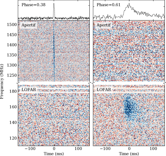
Figure Figure 1: Composite dynamic spectra of bursts A13 and L06 at Apertif and LOFAR frequency bands. The burst on the left (A13) was detected on MJD 58980.52593337 (barycentric), corresponding to a 0.38 activity phase. It is detected only in Apertif’s frequency band, with no emission below 190 MHz. The burst on the right (L06) was detected on MJD 58951.5416274, corresponding to a 0.61 activity phase. It is only detected in the LOFAR frequency band. The top panel of each burst shows their respective pulse profiles.

Previous low-frequency searches for FRBs have been unsuccessful, whether all-sky[14, 15] or targeted on known repeaters[2]. Such long campaigns (over a thousand hours on sky in total) resulted in strict limits on FRB emission below 300 MHz. Such upper limits fueled FRB theories in which free-free absorption around the emitter or strong intervening scattering was required. The nine LOFAR bursts at 120–190 MHz presented here are the first FRB detections in this frequency range. The pulse profiles, spectra and dynamic spectra of the nine bursts are presented in Figure 2, and their properties are summarised in Extended Table 1. All had simultaneous Apertif coverage, but no bursts were detected there down to a limit of 0.5 Jy ms.

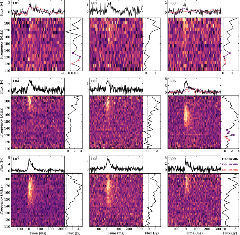
Figure Figure 2: Dynamic spectra of the nine bursts from FRB 20180916B detected with LOFAR, dedispersed to the S/N maximizing LOFAR DM of 349.00 pc cm^-3. For each burst, the top panel shows the calibrated pulse profile, the right panel the spectrum and the bottom left panel the dynamic spectrum. In bursts L01, L03, and L06, where there is evidence of emission below 140 MHz, the pulse profiles between 130 MHz and 140 MHz are plotted in purple, and between 120 MHz and 130 MHz are plotted in pink. The dynamic spectra were respectively downsampled by factors 2 and 64 in time and frequency for bursts L01–L03, and by factors 2 and 32 in time and frequency for bursts L04–L09.

Remarkably, for bursts of the same fluence, FRB 20180916B is around over an order of magnitude more active at 150 MHz than at 1.4 GHz, as seen in Extended Figure 1. Our detections allow for the first bounded constraints on the FRB all-sky rate below 200 MHz. A lower limit is obtained by assuming FRB 20180916B is the only source in the sky emitting at these frequencies. Combining this with previously published upper limits, we find that there are 3–450 sky^-1 day^-1 above 50 Jy ms at 90$\%$ confidence. Assuming an Euclidean fluence scaling, this is equivalent to 90–14000 sky^-1 day^-1 above 5 Jy ms at 150 MHz, which is promising for future high-sensitivity low-frequency surveys.

The integrated pulse shapes of the LOFAR bursts in Figure 2 are dominated by a sharp rise plus a scattering tail. We obtain a scattering timescale $\tau_{\mathrm{sc}}$=46$\pm$10 ms at 150 MHz, scaling with frequency as $\tau_{\mathrm{sc}}$$\propto\nu^{-4.2\pm 1.1}$. This is consistent with the frequency scintillation found for the same source at 1.7 GHz. For the typical $\nu^{-4}$ scaling, the $\sim$60 kHz decorrelation bandwidth seen there[9] translates to a $\sim$45 ms scattering time at 150 MHz. This scatter broadening may explain why none of the millisecond-duration frequency-time subcomponents seen at higher frequencies[16] are visible in the dynamic spectra in Figure 2. The observed scattering time is within a factor of two of the predicted Galactic scattering[17]. Thus, we attribute this pulse broadening to scattering in the Milky Way ISM and not plasma in the host galaxy. The fact that the ISM scattering is stronger in the Milky Way than in the host galaxy is not surprising, given FRB 20180916B is at a low galactic latitude, whereas its host is a nearly face-on spiral galaxy [9]; it is, however, notable that the environment local to the source scatters the FRB by $\lesssim$ 7 $\mu$s at 1.4 GHz. The dispersion measure (DM) of the bursts, $\text{DM}_{\text{LOFAR}}$ =349.00$\pm$0.02 pc cm^-3 , is in excess of previous DM measurements of the same source, which we interpret as an additional hint for the presence of unresolved subcomponents and not a frequency-dependent DM.

The dynamic spectra in Figure 2 show emission from the top of the band at 190 MHz down to 120 MHz for burst L01 and L07. As the LOFAR sensitivity decreases towards the bottom of the band, we cannot confidently rule out the presence of emission below 120 MHz. Our ability to detect these bursts at frequencies this low shows that free-free absorption and induced Compton scattering (ICS) do not significantly impact burst propagation for this source. Below we discuss the physical constraints for a number of models in greater detail. Combining these results with the small local RM and DM contribution, as well as the lack of temporal scattering, we do conclude here that some FRBs reside in clean environments, which is a prerequisite for some FRB applications to cosmology[18].

In our Apertif campaign, we detected 54 bursts. Ten of these had LOFAR coverage, but no bursts were detected there down to a fluence of 30 Jy ms. Half of the Apertif bursts have stored polarisation data, giving us access to the Stokes parameters and the polarisation position angle (PA) at multiple cycle phases. The pulse profiles, dynamic spectra of total intensity data and PA, where available, of all 1.4 GHz bursts are shown in Extended Figure 2, and their properties are summarised in Extended Table 2. All bursts are $\sim$100% linearly polarised, and the PA is constant within a single burst. The PAs are also relatively flat as a function of activity phase, and between cycles. This observation can be used to constrain the FRB emission mechanism, as well as the origin of periodic activity. A large fraction of the 1.4 GHz bursts show multiple subcomponents with a noticeable downward drift in frequency. We estimated each burst DM by maximising the burst structure [3, 16]. This gives similar results as the S/N maximisation technique for single component bursts, but is of particular importance in bursts with complex morphologies. From the brightest bursts (S/N>20), we get the best $\text{DM}_{\text{Apertif}}$ =348.75$\pm$0.12 pc cm^-3. This value is consistent with previous structure maximising DM measurements of the source and limits its DM derivative to less than 0.05 pc cm^-3 yr^-1.

The downward drift in frequency of the burst subcomponents is a phenomenon that has been previously observed in FRB 20180916B, and seems to be common among repeating FRBs[16, 3, 6, 8]. However, drift rate measurements of FRB 20180916B previous to this work had been estimated below 800 MHz with a value of $\dot{\nu}=-4.2\pm 0.4$ MHz ms^-1at 400 MHz[2] and an average of $-21\pm 3$ MHz ms^-1at 600 MHz[19]. We obtain an average drift rate at 1370 MHz of $-39\pm 7$ MHz ms^-1. This value is nine times larger than the drift rate at 400 MHz. The fitted drift rates are consistent with evolving linearly as a function of frequency. The same linear evolution of the drift rate with frequency has been observed in FRB 20121102A [20].

Our observations at 1.4 GHz covered the entire 16.35 day activity cycle to best investigate the periodicity. At 150 MHz we focused on the expected peak active time to maximise the detection probability. In Figure 3 this coverage is plotted, together with the arrival time of the bursts reported here and at other facilities[21, 22]. Our goal with the Apertif observations was to find or rule out any potential aliasing of the period. That possibility remained given the short daily source exposures at CHIME/FRB. Follow-up by other instruments across the predicted activity peak had not been able to rule out this aliasing (See Extended Figure 3). From the arrival MJD of Apertif, CHIME/FRB and all other detections, we built periodograms[23] from which we are able to confirm that the best period is 16.29${}^{+0.15}_{-0.17}$ days. This is the only period for which no bursts lie outside of a 6.1 day activity window including frequencies from 110 MHz to 1765 MHz, thus minimising the activity width fraction. We searched for short periodicity in both the Apertif and LOFAR observations, but found no significant period between 1 ms and 80 s.

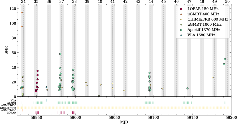
Figure Figure 3: Signal-to-noise ratio of the FRB 20180916B detections as a function of MJD (top) and duration of the observations of each instrument as a function of MJD (bottom). Here and in subsequent Figures, Apertif is always shown in green and LOFAR always in dark red. Detections by other instruments during the covered activity windows are plotted for comparison: uGMRT[22] at 400 MHz (orange), CHIME/FRB (yellow), uGMRT[21] at 650 MHz (lime) and VLA[23] (blue). The gray shaded regions correspond to the predicted activity days for a period of 16.35 days, with the predicted peak day as a dashed vertical line. The numbers on top of the plot indicate the cycle number since the first CHIME/FRB detection.

Apertif bursts were found in six out of the seven covered activity cycles, whereas all LOFAR bursts were detected in the activity window with no Apertif detections. However, the Apertif observations during the activity cycle with no Apertif detections started later in phase. We observe that most Apertif bursts arrive before CHIME/FRB’s activity peak day while LOFAR bursts arrive after. Previous observations of FRB 20180916B had hinted at a frequency dependence of the activity window[4]. Nevertheless, the scarcity of bursts detected outside of the frequency band covered by CHIME/FRB did not allow for a precise characterisation of the activity window at different frequencies. Using the Apertif, LOFAR and CHIME/FRB burst samples, we have evaluated the activity windows at 1.4 GHz, 600 MHz and 150 MHz respectively. Using the arrival phase of the bursts with a 16.29 day period (Figure 4, see Methods), we calculate the burst rate at each instrument as a function of phase. We find that the activity window is narrower and peaks earlier at 1.4 GHz than at 600 MHz. The peak activity at Apertif is $\sim$ 0.7 days before that of CHIME/FRB and its full-width at half-maximum (FWHM) is 1.1 days compared to CHIME/FRB’s 2.7 days. The LOFAR activity cycle appears to peak $\sim$2 days later than CHIME/FRB’s, but the lower number of detections does not allow for a better activity window estimate. It is not yet clear if this effect is discrete, akin to the drifting sub-pulses but on longer timescales, such that for a given frequency range the activity window peaks at the same time. Alternatively, it could be continuous in frequency analogous to dispersion; analyzing the peak frequency of the CHIME/FRB bursts as a function of activity phase would help answer this question. We evaluated the likelihood of the bursts being drawn from the same distribution, taking into account the survey strategy. We can discard the Apertif-CHIME/FRB and Apertif-LOFAR burst samples as being drawn from the same distribution with a $>$ $3\sigma$ confidence, and the CHIME/FRB-LOFAR samples with a $>2\sigma$ confidence (see Methods and Extended Figure 4).

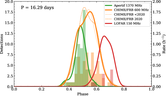
Figure Figure 4: Activity windows as a function of phase for a period of 16.29 days for Apertif (green), CHIME/FRB (orange) and LOFAR (red). The histograms represent the number of detections and the solid lines the rate obtained with kernel density estimates. The orange dotted line is the KDE for CHIME/FRB bursts before 2020, and the dashed line for CHIME/FRB bursts in 2020, establishing that the wider activity window is not due to the longer time baseline for CHIME.

The initial discovery of periodic activity in FRB 20180916B led to many new models to explain this source. The subsequent detection of a possible 160 day period in FRB 20121102A [24] led to further enthusiasm for periodicity models. One category of models places the engine of FRB 20180916B – a pulsar or magnetar – in a binary system with a $\sim$16 day orbital period, where the companion wind obscures the coherent radio emission for most of the orbit via free-free absorption. The companion can be either a massive star or another neutron star[25, 26]. In these models, a frequency-dependent activity window is predicted but with wider phase ranges at high frequencies because such absorption effects are stronger at longer wavelengths. Additionally, these models predict a DM evolution due to the dynamic absorption column, as well as a low-frequency cutoff. Our observations of a smaller phase range at higher frequencies, constant DM, and emission down to 120 MHz challenge all three predictions of this model. With the data presented in this work, binary wind models are highly disfavored as an explanation to the periodicity of FRB 20180916B.

Another set of models centers on a precessing magnetar, where the periodic activity of the FRB follows the precession period. Th precession is either free if the magnetar is isolated[27] or forced if, for example, it has a fallback disk[28]. Precessing models predict that a second, shorter periodicity from the neutron star rotation itself is detectable in the pulse train within an activity window. We find no such intra-window periodicity. Mechanisms such as spin noise, pulse profile instability, and dephasing of the burst beams are to be expected in young magnetars however, and these could conceal the underlying rotation period. In these models, if the FRB is produced as the neutron star (NS) beam rotates, a PA sweep is expected[27]. We instead observe a flat PA. Furthermore, free precession models typically require young, hot, and highly active magnetars which may still be embedded in their birth environment. The limits we set on local scattering, absorption, and DM variation suggest, however, that FRB 20180916B is no longer surrounded by a dense supernova remnant and any remaining magnetar wind is not hampering radio propagation.

A precessing magnetar could also be responsible for the periodicity of FRB 20180916B if its coherent radio emission is produced farther out. In synchrotron maser shock models[29] a flare from the central magnetar causes an ultra-relativistic shock when colliding with the neighboring medium. The FRB emission is produced in this magnetized shock. This model predicts the flat, constant intra-burst PAs we observe, perpendicular to the upstream magnetic field of the surrounding material. But it is not clear if such models can power emitters as prolific as FRB 20180916B and FRB 20121102A. The absence of short periodicity and DM variation with phase is consistent with the ultra-long period magnetar (ULMP) scenario[30]. That model, however, requires expelling enough angular momentum to produce a period that is five orders of magnitude larger than any definitively-known neutron star rotation period.

Methods

A high-level description of the observational and analysis methods is found below. Further detail following the same order is provided in the Supplementary Methods.

1 Observations and burst search

1.1 Apertif

The Westerbork Synthesis Radio Telescope (WSRT) is a radio interferometer located in Drenthe, the Netherlands, consisting of twelve 25-m dishes in which a new system called Apertif (Aperture Tile in Focus) has recently been installed. Single receivers have been replaced by phased array feeds (PAFs), increasing its field of view to $\sim$8.7 square degrees[31, 32]. Apertif can work in time-domain observing mode to search for new FRBs[33] and follow-up known ones[34] using eight of the WSRT dishes. This capability is provided by a new backend, ARTS (the Apertif Radio Transient System[35, 11, 36]). ARTS covers the full Apertif field-of-view with up to 3000 tied-array beams, each with a typical half-power size of 25’ by 25". In real-time FRB searches, the system records Stokes I data at a central frequency of 1370 MHz and a 300 MHz bandwidth with 81.92 $\mu$s and 195 kHz time and frequency resolution. The data are then searched in near-real time with our burst search software AMBER[37, 38, 39] and post-processing software DARC[40]. Raw FRB candidates are then filtered by a machine learning algorithm that assigns a probability of the candidate being of true astrophysical origin[41] and later checked by human eyes. When AMBER identifies an FRB candidate with a duration $<$10 ms, a signal-to-noise ratio (S/N) >10 and a dispersion measure (DM) 20% larger than the expected Milky Way contribution to the DM in the pointing direction according to the YMW16 model[42], the full Stokes IQUV data of the candidate is saved. When following up known sources, the system also stores Stokes IQUV for any candidate with S/N > 10 and a DM within 5 pc cm^-3 of the source DM.

We carried out observations of FRB 20180916B with Apertif, resulting in 388.4 h on source. The observations covered seven of the predicted 16.35 days activity cycles of FRB 20180916B, and the exposure times are visualised in the bottom panel of Figure 3. The observations of the three activity cycles after our first detection (numbered 35,37 and 38) ranged over the whole activity phase instead of only at the predicted active days in order to rule out or confirm any potential aliasing of the period[4]. The later observations were scheduled at the confirmed activity peak days.

1.2 LOFAR

The LOw Frequency ARray (LOFAR[43, 12]) is an interferometric array of radio telescopes whose core is located in Drenthe, the Netherlands. LOFAR was used to obtain 57.6 h of beam-formed data between 110 and 188 MHz, simultaneous to Apertif observations. LOFAR observations were taken at the predicted active days to increase the chances of detecting bursts that are broad band from 1.4 GHz to 150 MHz, at both telescopes.

The observations were taken during commissioning of the transient buffer boards (TBBs) at LOFAR. In this observing mode, up to five dispersed seconds of raw sub-band data can be saved when a trigger is sent from another instrument. During the simultaneous Apertif-LOFAR observations, if AMBER detected a burst with S/N>10 and a DM within five units of 349.2 pc cm^-3, Apertif sent a trigger to LOFAR. The dispersive delay between 1220 MHz (the bottom of the Apertif band) and 188 MHz (the top of the HBA band) gives enough time for the pipeline to find the candidate and send the alert, so that LOFAR can freeze the raw data in time.

All the LOFAR data were also searched offline for FRBs and periodic emission. After subbanding and RFI cleaning[44], data were dedispersed and searched for single pulses. Candidates were clustered in DM and time, visualized, and examined by eye.

2 Data analysis

2.1 Detected bursts

During our observing campaign, we detected a total of 63 bursts, 54 with Apertif and 9 with LOFAR. None of these detections took place simultaneously at both instruments. Figure 3 shows the S/N of each detection as a function of modified julian day (MJD). It includes the detections by other instruments during the same time span for comparison, and the observation times in the bottom panel. The predicted activity days for a period of 16.35 days are illustrated as shaded regions in order to guide the eye, and the cycle number since the first CHIME/FRB detection are indicated on top.

2.2 Bursts detected with Apertif

We detected a total of 54 bursts with an S/N above 8 in 388.4 h of observations with Apertif. All Apertif bursts are given an identifier AXX, where XX is the burst number ordered by time of arrival within the Apertif bursts, from A01 to A54. Twenty-five of those bursts triggered a dump of the full-Stokes data. Eight of the bursts were not detected in real time, but in the later search of the filterbank observations with PRESTO. The number of IQUV triggers during cycle 44 is lower due to the incremented RFI environment that triggered IQUV dumps on RFI and avoided saving IQUV data on later real bursts. Extended Table 2 summarises the main properties of the detected bursts. The burst fluence distribution is further analyzed in the Supplementary Methods. All detections took place in six out of the seven predicted activity cycles that our observations covered. In spite of observing FRB 20180916B during five days centered at the predicted Apertif peak day during cycle 47, only one burst was detected, revealing that the burst rate can fluctuate from cycle to cycle. Extended Figure 2 shows the dynamic spectra and pulse profile of all bursts. Additionally, Stokes L and V are plotted for the bursts with full-Stokes data, together with the polarisation position angle (PA).

As shown in Figure 3, all Apertif bursts were detected in a four-day window before the predicted peak day of the corresponding activity cycle, with none of the detections happening after the peak. There were no detections outside of a six-day activity window, even though they were largely covered by our observations. The late start of the observations around MJD 58950 with respect to the beginning of the predicted activity window could explain the non-detections in that cycle. However, the lack of emission at 1.4 GHz during that cycle cannot be discarded. After our detections and non-detections during the first four cycles, we refined the expected active window time at 1.4 GHz and scheduled the observations of the last three cycles accordingly, in five-day windows centered at the predicted Apertif peak day.

The detected bursts present a large variety of properties. Some display a single component, others show rich time-frequency structure with up to five components.

2.3 Bursts detected with LOFAR

We detected a total of nine LOFAR bursts above a S/N of 7 in $\sim$58 h of observations The bursts occurred on 10, 11 and 12 April 2020. Each burst is given an identifier LYY, where YY is the burst number ordered by time of arrival within LOFAR bursts, from L01 to L09. Extended Table 1 summarises the properties of these bursts. The fluence scale was derived following previously established procedures[45, 46], detailed in the Supplementary Methods. As shown in Figure 3, all detections took place on the same predicted activity cycle in which there were no Apertif detections (cycle 35). The observations where the detections took place were performed in coherent Stokes I mode. Excepting the first two, all bursts arrived after the predicted peak day. There were thus no simultaneous bursts at 1.4 GHz and 150 MHz in the beamformed data nor the TBBs. From the dynamic spectra and pulse profiles displayed in Figure 2, there is no evidence of complex, resolved time-frequency structure. Nevertheless, a scattering tail is manifest in the pulse profiles of the brightest bursts. We will characterise the scattering timescale below. While the tail of burst L06 in Figure 1 appears to plateau 25 ms after the main peak, hinting for a second subburst, a fit for multiple scattered bursts did not confidently identify a second component.

Generally, the LOFAR-detected bursts are brightest in the top of the band (see Figure 2). Over the almost 2:1 ratio of frequency from that top of the band to the bottom, most bursts gradually become less bright. Although some previous targeted LOFAR FRB searches used wide bandwidths[47], most large-area searches were carried out in the lower part of the band, e.g., 119$-$151 MHz[14, 48] where LOFAR is more sensitive. The behavior we see here was likely a factor in the earlier lack of detections.

The detections reported here already demonstrate there is no low-frequency cutoff above the LOFAR band. The individual bursts and the stacked profile (Extended Figure 5) also do not show a clear cutoff within the band. Two of the bursts (L01, L06) emit down to at least 120 MHz (see Extended Figure 6) and thus cover the entire frequency range. Furthermore, if we follow burst L06 from 150 to 120 MHz in decreasing frequency, the emission is ever more delayed with the respect to the onset of the peak (see Figure 1 and Figure 2). Such behavior suggests unresolved time-frequency downward drift in the tail of the pulse. From this we conclude the decrease in pulse peak brightness could be intrinsic, and is not due to a cutoff by intervening material. Bursts L04 and L05 show a similar hint of a delayed tail, at slightly higher frequencies.

2.4 Ruling out aliasing

To maximise the chance of detection, FRB 20180916B is generally observed predominantly around its predicted activity peak[2, 10, 23, 22]. The implied lack of coverage outside this purported peak could bias the derived activity cycle. The best-fit cycle period could be an alias of the true period. To break this degeneracy, we scheduled observations covering full activity cycles (see Supplementary Methods). We find there is no aliasing. We determined a new best activity period of 16.29 days, where reference MJD 58369.9 centered the peak activity day at phase 0.5.

2.5 Activity windows

By using the aforementioned best period and reference MJD to compute the burst arrival phases, we have generated a histogram of detections versus phase on the top panel of Extended Figure 3. The cycle coverage by different instruments can be visualised on the bottom panel of the same figure, where it is manifest that CHIME/FRB and Apertif are the only instruments covering the whole activity cycle which have detected bursts. We have used data from all FRB 20180916B observations published thus far[4, 9, 49, 10, 2, 21, 23, 50].

Several theoretical models have suggested the activity window may be frequency dependent[25, 26, 30]. In absorptive wind models, for example, one expects a larger duty cycle at high frequencies due to heightened opacity at long wavelengths. There was also an observational hint that higher frequencies may arrive earlier, based on four EVN detections at 1.7 GHz[9]. By taking into account the bursts detected by Apertif, CHIME/FRB and LOFAR at 1.4 GHz, 600 MHz and 150 MHz respectively, we can obtain an estimate of the probability of the bursts being drawn from the same distribution at different frequencies.

To do so, we attempted to estimate the detection rate as a function of activity phase for the three different frequency bands. We estimate these activity windows by computing the probability density function (PDF) of detection rate for Apertif, CHIME/FRB and LOFAR using a weighted kernel density estimator (KDE, see Supplementary Methods).

We applied the KDE separately to the Apertif, CHIME/FRB and LOFAR burst datasets. Based on the KDE estimation shown in Figure 4, we find that higher frequencies appear to arrive earlier in phase, i.e. the activity peaks at a lower phase with larger frequencies. Additionally, the width of the activity window appears to be larger with CHIME/FRB. The KDE is useful for estimating probability distributions with a small number of samples, but it is non-parametric and does not easily allow us to compare the activity window widths between frequencies. For this we fit a Gaussian to the detection rate of FRB 20180916B for each instrument and find a full-width at half maximum (FWHM) of 1.2$\pm$0.1 days from the Apertif data at 1370 MHz and 2.7$\pm$0.2 days at 400–800 MHz using the CHIME/FRB bursts. The best-fit peak activity phase for Apertif is 0.494$\pm$0.002 and 0.539$\pm$0.005 for CHIME/FRB. The source activity window is therefore roughly two times wider at CHIME/FRB than at Apertif and its peak is 0.7 days later at CHIME/FRB. We do not attempt to fit a Gaussian to the LOFAR bursts because of the small number of detections and our limited coverage in phase. However, we note that four out of the nine detected LOFAR bursts arrive later in phase than every previously detected CHIME/FRB burst. Therefore, the activity of FRB 20180916B at 150 MHz likely peaks later than at higher frequencies and the activity window may be wider as well. This is in stark contrast with the predictions of simple absorptive wind models where the activity ought to be wider at higher frequencies.

By applying a Kolmogorov-Smirnov test to the burst samples of Apertif, CHIME/FRB and LOFAR comparing them two by two and taking into account the different observing strategies, we can discard the Apertif and CHIME/FRB burst samples as being drawn from the same distribution with a three-sigma confidence level, as well as the Apertif and LOFAR burst samples. For the CHIME/FRB and LOFAR bursts, the confidence level of the samples being drawn from different distributions is greater than two sigma. This method is expanded in the Supplementary Methods section.

Taking all observational biases into account, a dependence of the activity window with frequency must exist in order to get the observed burst distribution, which is narrower and peaks earlier in phase at higher frequencies. This is opposite to the predictions made by binary wind model predictions in which free-free absorption would make the lower frequency emission have a narrower activity width[25, 26], and thus disfavors the cause of the periodicity to be free-free absorption in a binary system.

2.6 Polarisation

Monitoring the polarisation position angle (PA) of FRB 20180916B over time and across cycles with Apertif is made easier by the fact that Westerbork is a steerable equatorial mount telescope. This stability of the system’s response allows us to investigate the polarisation properties of FRB 20180916B within each pulse, within an activity cycle, and even between multiple periods. After calibration (see Supplementary Methods) we find the PA of FRB 20180916B to be flat within each burst, with $\Delta$PA<20 deg, in agreement with other polarised studies of the source[8, 2, 51]. This is in contrast to most pulsars whose PAs swing across the pulse, in many cases with the S-shaped functional form predicted by the rotating vector model (RVM). In the classic picture, PA varies with the arctangent of pulse longitude and the amount of swing is proportional to the emission height but inversely proportional to the star’s rotation period[52]. However, the flat PAs of FRB 20180916B are similar to other FRBs, notably FRB 20121102A whose intra-burst polarisation exhibits less than 11 deg of rotation[3]. They are also similar to radio magnetars. FRB 181112 was the first source to show significant variation in the polarisation state within a burst and between sub-components of an FRB with temporal structure[53].

While the flat PAs within each FRB 20180916B burst are in line with previous measurements, we have found that its PA is also stable in average within an activity cycle and even between periods, with $\Delta$PA<40 deg. In models that invoke precession as the origin of periodicity and magnetospheric emission as the origin of the FRBs, one generically expects a PA change as a function of activity phase. However, the amount of PA swing depends on the geometry of the system and well as the fraction of a precession period that is observable[27], so we cannot rule out precession with our polarisation measurements. In relativistic shock models, the synchrotron maser mechanism provides a natural path for flat PAs within a burst, but it is not clear how or if the polarisation state could be nearly constant within a cycle and over multiple months[29, 54]. Given the duty cycle of FRB 20180916B appears to be just $\sim$10$\%$ in the Apertif band, it will be useful to observe the PAs of FRB 20180916B over at lower frequencies with a steerable telescope that can cover a full periodic cycle.

2.7 Dispersion

The Apertif real-time detection pipeline finds the dispersion measure that maximises the S/N of a burst ($\mathrm{DM}_{\mathrm{S/N}}$). Any frequency-swept structure intrinsic to the pulse, as seen in a number of repeating FRBs, will be absorbed in this value. By first fitting to such structure[3, 16] the interstellar dispersion measure can be isolated, and reported as $\mathrm{DM}_{\mathrm{struct}}$ . We thus determined $\mathrm{DM}_{\mathrm{struct}}$ for all Apertif bursts (see Supplementary Methods) and find it to be $\text{DM}_{\text{Apertif}}$ =348.75$\pm$0.12 pc cm^-3, consistent with previous findings. There is no evidence for a variation of DM with phase (Extended Figure 7, top panel).

The LOFAR bursts lack detectable time-frequency structure, but require separating the frequency-dependent scattering tails from the DM fit (see Supplementary Methods). For the final LOFAR DM, obtained by averaging over all bursts with S/N>20 (Extended Table 1), we find $\text{DM}_{\text{LOFAR}}$ $=349.00\pm 0.02$ pc cm^-3 .

2.8 Sub-pulse drift rate

Several of our detections at Apertif show downward drifting sub-pulses, enabling us to make the first measurement of the drift rate $\dot{\nu}$ of FRB 20180916B above 1 GHz (Extended Figure 8). We obtain an average sub-pulse drift rate of $-39\pm 7$ MHz ms^-1  at 1370 MHz. This is nine times larger than e.g. the previously reported drift rate of $\sim-$4.2 MHz ms^-1at 400 MHz[2]. Extended Figure 9 shows how the downward drift amplifies towards higher frequencies. As in FRB 20121102A [20], the drift rate evolution appears linear. As these two FRBs reside in significantly different environments, the behavior may be common across FRBs. The frequency-dependence and consistent sign of the drifting phenomenon will likely offer clues to the FRB emission mechanism[29, 55, 56].

2.9 Scattering

Most of the LOFAR bursts (Figure 2) exhibit an exponential tail, indicating the pulse-broadening due to scattering in the intervening medium. To quantify the scatter broadening timescale ($\tau_{\mathrm{sc}}$), we divided the dedispersed spectrograms of a few high S/N bursts into 4 or 8 sub-bands The burst profiles obtained from the individual sub-bands were modelled as a single Gaussian component convolved with a one-sided exponential function[57, 58]. The $\tau_{\mathrm{sc}}$thus obtained are presented in Extended Table 1.

In order to obtain a more precise estimate of scatter-broadening timescale, we first divided the bandwidth of the stacked LOFAR bursts dedispersed to their $\text{DM}_{\text{LOFAR}}$ =349.0 pc cm^-3 into eight frequency bands, for which we obtained separate pulse profiles and fitted each to a scattering tail as above. The results are shown in Extended Figure 5. We obtain the scattering timescale of 45.7$\pm$9.5 ms at 150 MHz, which is consistent with the measurements using individual bursts. We also characterize the scatter broadening variation with frequency as $\tau_{\mathrm{sc}}$$\propto\nu^{-\alpha}$ and obtain the frequency scaling index $\alpha=-4.2$${}^{+1.1}_{-1.0}$. This scatter-broadening is consistent with the upper limit of 50 ms at 150 MHz that was derived from GBT detections at 350 MHz[2]. By scaling the scatter broadening of LOFAR bursts to Apertif frequencies, we expect $\tau_{\mathrm{sc}}$ $\sim 6.6\mu$s at 1370 MHz, which is an order of magnitude smaller than Apertif’s temporal resolution.

2.10 Rates

Before our LOFAR detections, there existed only upper limits on the FRB sky rate below 200 MHz. Blind searches for fast transients at these low frequencies are difficult due to the deleterious smearing effects of intra-channel dispersion and scattering, which scale as $\nu^{-3}$ and $\nu^{-4}$, respectively. This is amplified by the large sky brightness temperatures at long wavelengths, due to the red spectrum of Galactic synchrotron emission; pulsars are detectable at low frequencies because of their steeply rising negative spectra, but the spectral index of the FRB event rate is not known. We first consider the repetition rate of FRB 20180916B from our LOFAR and Apertif detections to determine its activity as function of frequency. We then convert that into a lower-limit on the all-sky FRB rate at 150 MHz and combine it with previous upper-limits at those frequencies to derive the first ever bounded constraints on FRB rates below 200 MHz.

We detected nine bursts in 58 hours of LOFAR observing, giving a rate of 0.16 $\pm 0.05$ h^-1. Since we only targeted LOFAR during simultaneous Apertif observations during the presumed activity window whose duty cycle is $\sim$0.25, we divide this rate by 4 to get its repetition rate averaged over time. Assuming a fluence threshold of 50 Jy ms and noting that the duration of all bursts from this source at 150 MHz is set by scattering and does not vary, we find $R_{150}(\geq\,50\,\rm{\,Jy\,ms})\approx(3.9\pm 1.3)\times 10^{-2}$ h^-1. At 1370 MHz, Apertif detected 54 pulses in 388 hours of observing. Our coverage of FRB 20180916B was deliberately more uniform in activity phase, so only $\sim$149 h took place during the active days. The phase range in which Apertif detected bursts gives a duty cycle of 0.22. This results in $R_{1370}(\geq 1\,\rm{\,Jy\,ms})\approx(8.0\pm 1.1)\times 10^{-2}$ h^-1. While the absolute detection rates by Apertif and LOFAR are similar, we note that the fluence threshold was much lower for Apertif than LOFAR. Scaling by the known fluence distribution of FRB 20180916B, $N(\geq\mathcal{F})\propto\mathcal{F}^{-1.5}$, we find $R_{1370}(\geq 50\,\rm{\,Jy\,ms})\approx 2.3\times 10^{-4}$ h^-1. We come to the remarkable conclusion that the FRB is more active at 150 MHz than at 1370 MHz at the relevant fluences.

The all-sky FRB event rate is a difficult quantity to determine for a myriad of reasons[59]. Beam effects result in a pointing-dependent sensitivity threshold, which in turn is affected by the unknown source-count slope[60, 61]; Each survey has back-end dependent incompleteness, including in flux density and fluence[62] as well as in pulse duration and DM[63]. Nonetheless, meaningful constraints can be made if one is explicit about the region of parameter space to which the rate applies.

As the LOFAR bursts are the sole unambiguous FRB detections below 200 MHz, we and other teams[13] can now provide the first bounded limits on the all-sky event rate at low frequencies. A lower limit on the FRB rate at 150 MHz can be obtained by assuming FRB 20180916B is the only source in the sky emitting at these wavelengths. This lower bound can be combined with previous upper bounds from non detections by blind searches at LOFAR and MWA[15, 14, 64, 65, 66, 67]. The repetition rate of FRB 20180916B implies that there are at least 0.6 sky^-1 day^-1 above 50 Jy ms at 110–190 MHz at 95$\%$ confidence. Assuming a Euclidean scaling in the brightness distribution that continues down to lower fluences, this is equivalent to more than 90 sky^-1 day^-1 above 5 Jy ms. An earlier blind LOFAR search[15] placed an upper limit of 29 sky^-1 day^-1 above 62 Jy pulses with 5 ms duration. Combining these two limits, we obtain a 90$\%$ confidence region of 3–450 sky^-1 day^-1 above 50 Jy ms.

The lower-limit value may be conservative, as FRB 20180916B is in the Galactic plane at a latitude of just 3.7 $\deg$, which is why its scattering time is 50 ms at 150 MHz. If the burst width were 5 ms before entering the Milky Way, then a factor of $\sim$3 was lost in S/N due to the low Galactic latitude of FRB 20180916B. Therefore, a similar FRB at a more typical offset from the plane would, in this example, be $\sim$3^γ times more active, where $\gamma$ is the cumulative energy distribution power-law index, because the Galactic scattering timescale would only be a few milliseconds.

3 Data availability

Raw data were generated by the Apertif system on the Westerbork Synthesis Radio Telescope and by the International LOFAR Telescope. The Apertif data that support the findings of this study are available through the ALERT archive, http://www.alert.eu/FRB20180916B. The LOFAR data are available through the LOFAR Long Term Archive, https://lta.lofar.eu/, by searching for “Observations” at J2000 coordinates RA=01:57:43.2000, DEC=+65:42:01.020.

References

This research was supported by the European Research Council under the European Union’s Seventh Framework Programme (FP/2007-2013)/ERC Grant Agreement No. 617199 (‘ALERT’), and by Vici research programme ‘ARGO’ with project number 639.043.815, financed by the Dutch Research Council (NWO). Instrumentation development was supported by NWO (grant 614.061.613 ‘ARTS’) and the Netherlands Research School for Astronomy (‘NOVA4-ARTS’, ‘NOVA-NW3’, and ‘NOVA5-NW3-10.3.5.14’). We further acknowledge funding from an NWO Veni Fellowship to EP; from Netherlands eScience Center (NLeSC) grant ASDI.15.406 to DV and AS; from National Aeronautics and Space Administration (NASA) grant number NNX17AL74G issued through the NNH16ZDA001N Astrophysics Data Analysis Program (ADAP) to SMS; by the WISE research programme, financed by NWO, to EAKA; from FP/2007-2013 ERC Grant Agreement No. 291531 (‘HIStoryNU’) to JMvdH; and from VINNOVA VINNMER grant 2009-01175 to VMI.
This work makes use of data from the Apertif system installed at the Westerbork Synthesis Radio Telescope owned by ASTRON. ASTRON, the Netherlands Institute for Radio Astronomy, is an institute of NWO.
This paper is based (in part) on data obtained with the International LOFAR Telescope (ILT) under project code COM_ALERT. These data are accessible through the LOFAR Long Term Archive, https://lta.lofar.eu/, by searching for “Observations” with the J2000 coordinates RA 01:57:43.2000 and DEC +65:42:01.020, or by selecting COM_ALERT in “Other projects” and downloading data which includes R3 in the “Observation Description”. LOFAR (van Haarlem et al. 2013) is the Low Frequency Array designed and constructed by ASTRON. It has observing, data processing, and data storage facilities in several countries, that are owned by various parties (each with their own funding sources), and that are collectively operated by the ILT foundation under a joint scientific policy. The ILT resources have benefitted from the following recent major funding sources: CNRS-INSU, Observatoire de Paris and Université d’Orléans, France; BMBF, MIWF-NRW, MPG, Germany; Science Foundation Ireland (SFI), Department of Business, Enterprise and Innovation (DBEI), Ireland; NWO, The Netherlands; The Science and Technology Facilities Council, UK; Ministry of Science and Higher Education, Poland.
We acknowledge use of the CHIME/FRB Public Database, provided at https://www.chime-frb.ca/ by the CHIME/FRB Collaboration.

IPM, LC, JVL, YM, STV, AB, LO, EP, SS and DV analysed and interpreted the data. IPM, LC, JVL, YM and STV contributed to the LOFAR data acquisition, and to the conception, design and creation of LOFAR analysis software. IPM, LC and JVL conceived and drafted the work, and YM, STV, AB, LO, EP, SS and DV contributed significant revisions. LO, JA, OB, EK, DVDS, AS, RS, EAKA, BA, WJDB, AHWMC, SD, HD, KMH, TVDH, BH, VMI, AK, GML, DML, AM, VAM, HM, MJN, TO, EO, MR and SJW contributed to the conception, design and creation of the Apertif hardware, software, and firmware used in this work, and to the Apertif data acquisition.

The authors declare that they have no competing financial interests.

Extended data

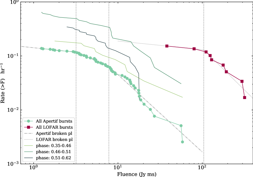
Figure Extended Figure 1: Cumulative distribution function of burst rate in fluence for both Apertif and LOFAR. The light green markers show the CDF of all Apertif bursts, with dash-dotted, dotted and dashed lines giving the power-law fit respectively to bursts with fluences lower than 3.2 Jy ms, between 3.2 and 7.8 Jy ms and above 7.8 Jy ms. The coloured solid lines correspond to different phase ranges within the active window, with no discernible difference between them other than the rate scaling. The LOFAR fluence distribution is shown in crimson. The fit to a broken power law with a fluence turnover at 104 Jy ms is shown as a gray dotted line. For the same fluence, FRB 20180916B is more active at 150 MHz than 1370 MHz, even at the peak activity phases observed by Apertif.

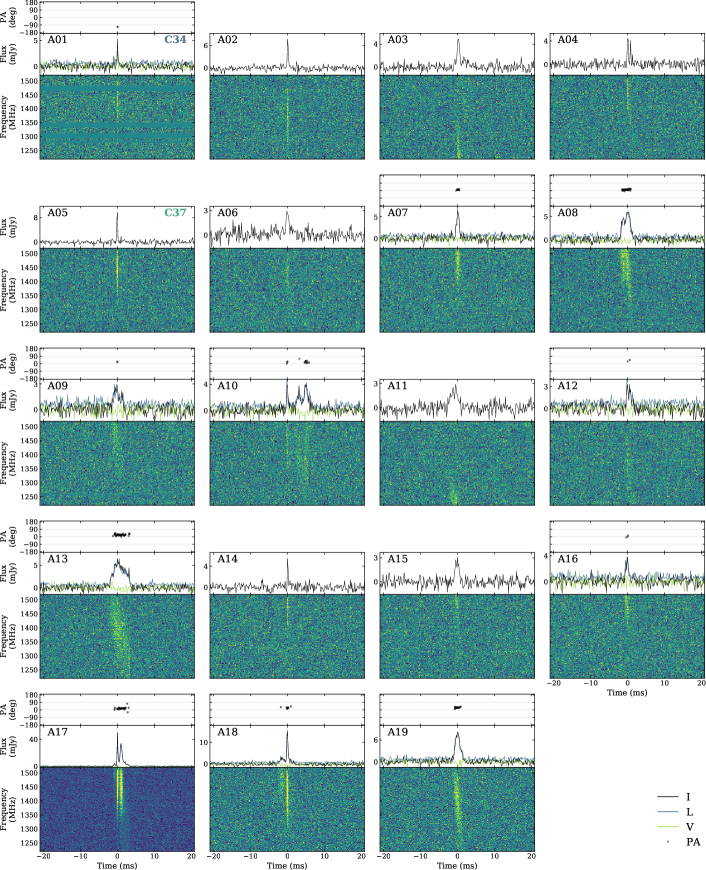
Figure Extended Figure 2: Dynamic spectra of the bursts (A01-A19) from FRB 20180916B detected with Apertif, dedispersed to a DM of 348.80 pc cm^-3. Bursts with full-Stokes data show PA (degrees) in the top panel, ILV in the central panel and dynamic spectrum in the bottom one. Bursts with only intensity data show pulse profile in the top panel and dynamic spectrum in the bottom one. The burst identifiers are given in the top left corner of the pulse profiles. The dynamic spectra have been downsampled by factors 2 and 8 in time and frequency. The activity cycle number is indicated on the top right corner of the first detected burst of each cycle.

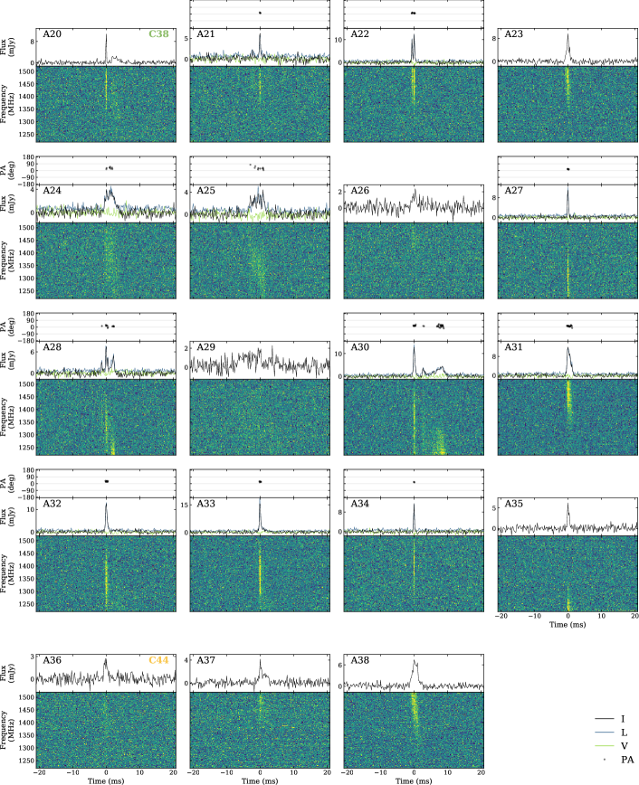
Figure Extended Figure 2: Continued, bursts (A20-A38).

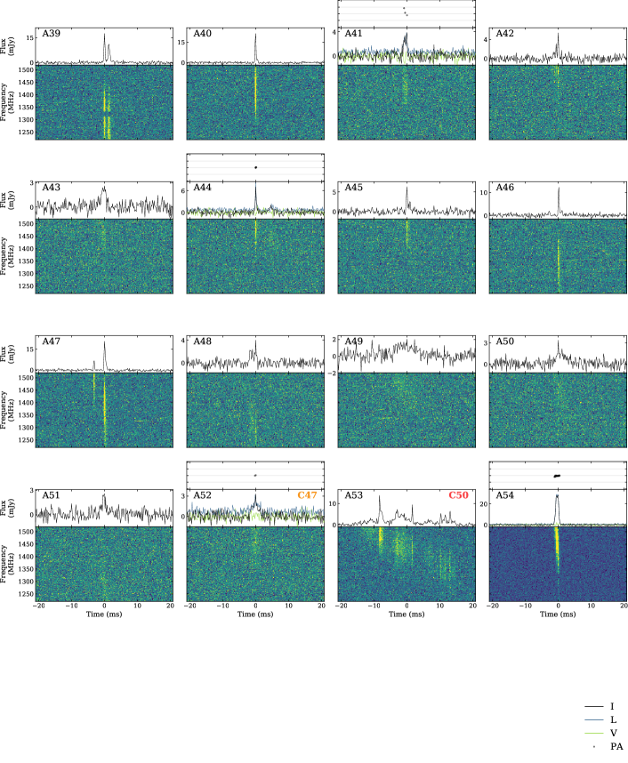
Figure Extended Figure 2: Continued, bursts (A39-A54).

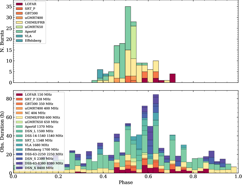
Figure Extended Figure 3: Histogram of burst detections (top) and observation duration (bottom) as a function of phase for the best period fitted to Apertif and CHIME/FRB data (16.29 days). Instruments are color-coded by central frequency, with blue for high frequencies and red for low frequencies. Figure was generated using an adaptation of the frbpa package[23].

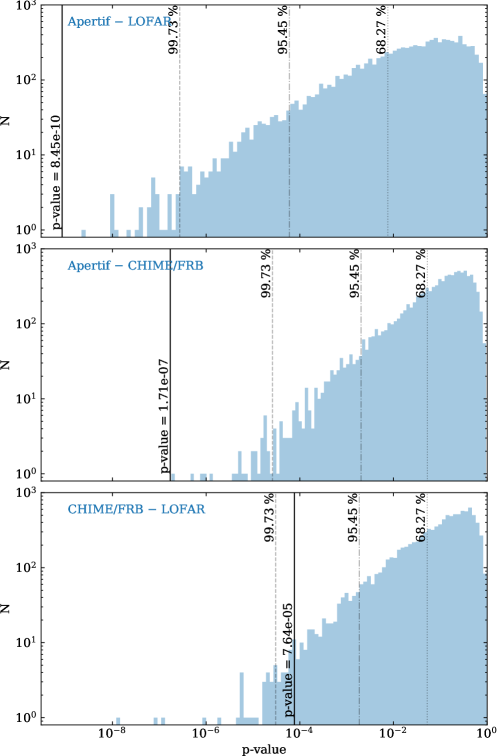
Figure Extended Figure 4: Comparison of simulated and observed activity window p-values. Each panel compares the p-value obtained through the Kolmogorov-Smirnov statistic on two instrument burst samples. The vertical black lines give the observed p-value, whereas the histograms correspond to 10000 simulations of the p-value that would be obtained if both instrument burst samples were drawn from the same distribution. The top panel compares the burst samples from Apertif and LOFAR, the central panel from Apertif and CHIME/FRB and the bottom panel from CHIME/FRB and LOFAR. The vertical gray dotted, dash-dotted and dashed lines show respectively the p-value where 68.27% (1$\sigma$), 95.45% (2$\sigma$) and 99.73% (3$\sigma$) of the simulations give a larger p-value.

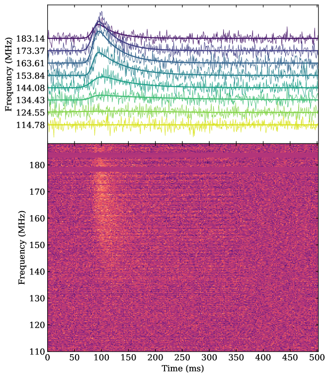
Figure Extended Figure 5: Stacked LOFAR bursts, dedispersed to the S/N maximising DM of 349.00 pc cm^-3. The top panel shows the pulse profiles in eight different frequency bands, and fits to the scattering tail. The central frequency of the band is indicated on the vertical labels. The bottom panel displays the dynamic spectrum of the stacked bursts.

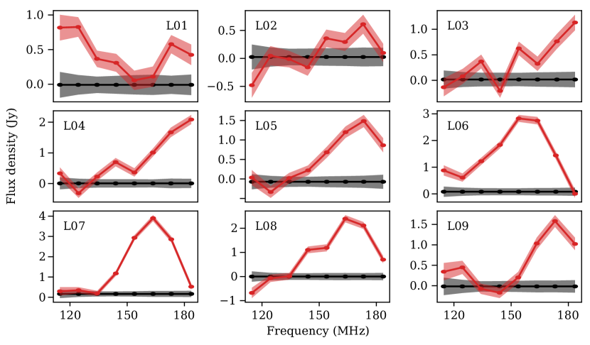
Figure Extended Figure 6: Comparison of the intrinsic LOFAR burst spectra to the telescope sensitivity limits. The red line shows the flux densities for the bursts, averaged over fixed [$-$50, +150] ms windows around the burst peak. The black line shows the same but for off-burst windows. The telescope sensitivity limits ($\pm 1\sigma$, black and red contours) calculated as the standard deviation of 3-s off-burst intervals, scaled to the 200-ms on-burst window. The LOFAR minimum detectable flux varies over the recorded band; it is higher at the band edges. The black contours demonstrate the response is relatively flat compared to the burst brightness. Note that this figure utilizes different frequency/time binning, which explains the apparent slight differences with Figure 2. Seemingly significant negative pulse flux densities at low frequencies in e.g. L02 and L08 were caused by slowly-varying, low-level residual RFI that affected the baseline subtraction. Nevertheless, bursts L01 and L06 clearly show emission above the noise level, at the lower edge of the LOFAR band.

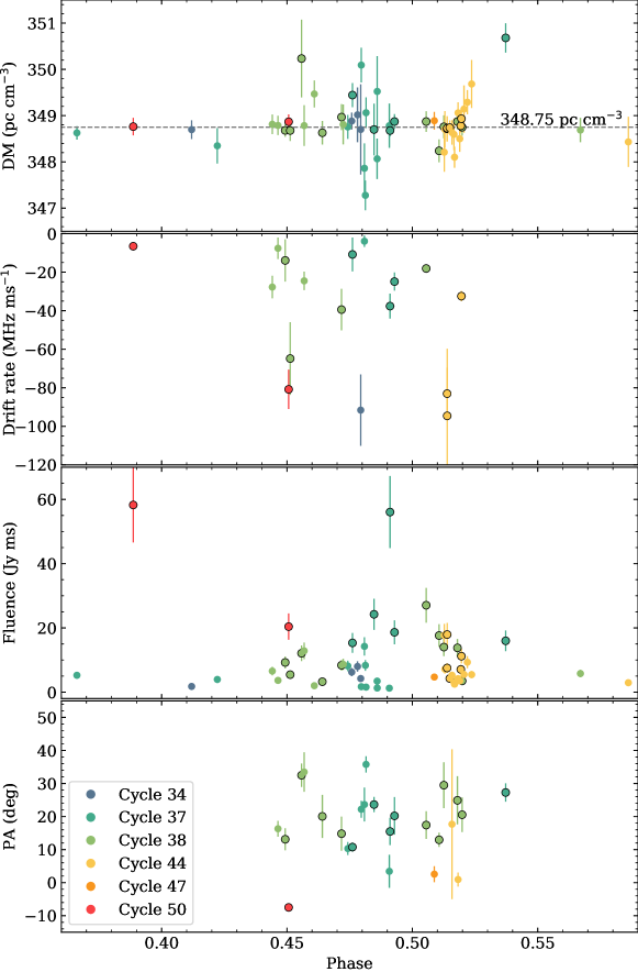
Figure Extended Figure 7: Apertif burst properties against phase. The top panel shows the structure optimised dispersion measure with the 348.75 pc cm^-3 average as a reference. The second panel shows the drift rate of bursts with multiple components. The third panel shows the fluence. The bottom panel gives the average polarisation position angle of each burst. Bursts are color-coded by activity cycle. Each color corresponds to a different activity cycle, and the data points with a black edge represent bursts with S/N>20.

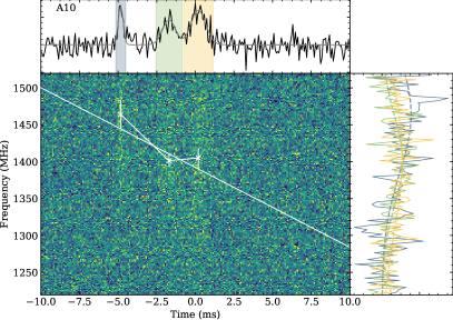
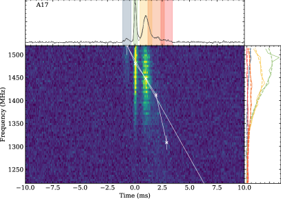
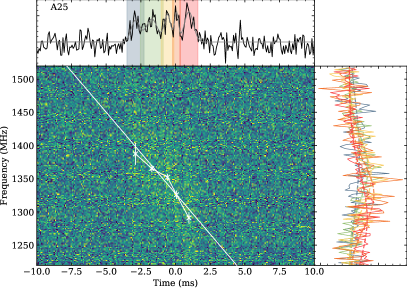
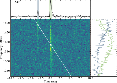
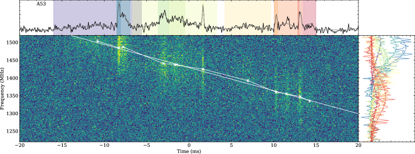
Figure Extended Figure 8: Five of the bursts with a measurable drift rate. For each burst, the top panel shows the pulse profile as a solid black line and the fitted multi-component Gaussian in gray, with shaded coloured regions indicating the position of the subcomponents. The lower left panels show the dynamic spectra rebinned eight times in frequency, with the centroid of each subcomponent and the fitted drift rate as a white line. The right panels represent the spectra and the fitted Gaussian of each subcomponent, with the same color as the shaded region of the pulse profile.

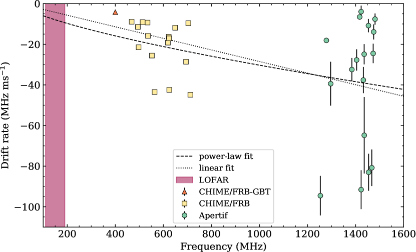
Figure Extended Figure 9: Comparison of drift rates at different frequencies. The green circles are the drift rate of bursts presented in this work, detected with Apertif. The yellow squares are drift rates from CHIME/FRB bursts[4, 19]. The orange triangle is the simultaneous CHIME/FRB-GBT burst where a drift rate was reported[2]. The dashed line is a power law fit of the drift rate at different frequencies, $\dot{\nu}=-0.2\nu^{0.7}$. The dotted line is the linear fit of the drift rate, $\dot{\nu}=-2.9\times 10^{-2}\nu$, and it is almost superposed to the power law fit.

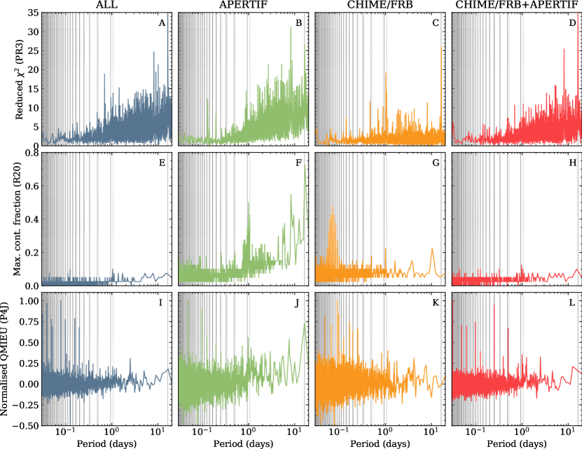
Figure Extended Figure 10: Periodograms between 0.03 day and 20 day periods of four instrument combinations and three different period searching techniques. Each column corresponds, from left to right, to all detections combined (blue), Apertif detections (green), CHIME/FRB detections (yellow) and CHIME/FRB and Apertif detections combined (red). Each column corresponds to a different search technique, with Pearson’s $\chi^{2}$ test at the top, activity width minimisation center, and QMI method at the bottom. The vertical gray lines mark the position of the aliased periods, solid for $f_{N}=(Nf_{\text{sid}}+f_{0})$ and dotted for $f_{N}=(Nf_{\text{sid}}-f_{0})$.

Extended Table 1: Summary of LOFAR burst properties.

Burst ID	OBSID	Arrival time	Arrival time	Detection	DM	Fluence	$\tau_{\mathrm{sc}}$at 150 MHz
		(MJD)	(UTC)	S/N	( pc cm-3 )	( Jy ms )	(ms)
L01	L775795	58949.53491816	2020-04-10 12:50:16.929	8.7	349.03$\pm$0.11	111$\pm$55	…
L02	L775801	58949.63987585	2020-04-10 15:21:25.273	7.3	348.94$\pm$0.08	38$\pm$19	…
L03	L775977	58950.52919335	2020-04-11 12:42:02.305	9.5	349.02$\pm$0.08	80$\pm$40	…
L04	L775977	58950.54130169	2020-04-11 12:59:28.466	18.9	349.41$\pm$0.03	177$\pm$88	…
L05	L775979	58950.58347838	2020-04-11 14:00:12.532	13.7	349.09$\pm$0.04	129$\pm$64	…
L06	L775953	58951.54162736	2020-04-12 12:59:56.604	29.4	349.03$\pm$0.05	318$\pm$159	48.2$\pm$16.6
L07	L775953	58951.55801455	2020-04-12 13:23:32.457	35.1	348.98$\pm$0.02	296$\pm$148	46.9$\pm$16.0
L08	L775955	58951.58470795	2020-04-12 14:01:58.767	23.5	348.99$\pm$0.03	193$\pm$96	36.2$\pm$19.0
L09	L775955	58951.59135120	2020-04-12 14:11:32.744	12.5	348.86$\pm$0.08	124$\pm$62	42.0$\pm$17.4

Extended Table 2: Summary of Apertif burst properties.

Burst ID	Arrival time	Arrival time	Detection	DM	Fluence	Drift rate
	(MJD)	(UTC)	S/N	( pc cm-3 )	( Jy ms )	( MHz ms-1)
A01	58930.47097294	2020-03-22T11:18:12.062	11.5	348.70(20)	1.8	…
A02	58931.51122577	2020-03-23T12:16:09.907	12.7	348.88(18)	6.2	…
A03	58931.54877968	2020-03-23T13:10:14.564	13.4	349.02(59)	8.0	…
A04	58931.56964778	2020-03-23T13:40:17.568	13.4	348.70(97)	4.2	…
A05	58978.59561357	2020-05-09T14:17:41.012	13.6	348.63(14)	5.2	…
A06	58979.50785914	2020-05-10T12:11:19.030	8.9	348.35(38)	4.0	…
A07	58980.35572077	2020-05-11T08:32:14.275	16.4	348.75(26)	8.2	…
A08	58980.38590828	2020-05-11T09:15:42.475	29.9	349.44(26)	15.3	-9.16
A09	58980.44318898	2020-05-11T10:38:11.528	13.9	350.09(37)	1.7	…
A10	58980.46375074	2020-05-11T11:07:48.064	17.8	347.86(54)	14.2	-3.95
A11	58980.46995949	2020-05-11T11:16:44.500	10.1	347.28(32)	8.3	…
A12	58980.47426015	2020-05-11T11:22:56.077	11.0	349.06(33)	1.6	…
A13	58980.52593337	2020-05-11T12:37:20.643	38.6	348.70(56)	24.2	…
A14	58980.54629988	2020-05-11T13:06:40.310	14.0	348.07(44)	3.4	…
A15	58980.54684270	2020-05-11T13:07:27.209	12.5	349.52(76)	1.3	…
A16	58980.62542392	2020-05-11T15:00:36.627	11.5	348.78(48)	1.2	…
A17	58980.62998094	2020-05-11T15:07:10.353	58.1	348.68(13)	56.0	-26.36
A18	58980.65889322	2020-05-11T15:48:48.374	25.6	348.87(16)	18.6	-18.12
A19	58981.38138907	2020-05-12T09:09:12.016	31.5	350.68(32)	16.0	…
A20	58996.15501128	2020-05-27T03:43:12.975	12.1	348.81(21)	6.6	-10.01
A21	58996.19203445	2020-05-27T04:36:31.776	12.7	348.79(21)	3.7	-3.56
A22	58996.23898191	2020-05-27T05:44:08.037	20.2	348.68(14)	9.2	-8.83
A23	58996.27129126	2020-05-27T06:30:39.565	20.9	348.68(23)	5.5	-42.74
A24	58996.34499129	2020-05-27T08:16:47.247	21.4	350.23(84)	12.1	…
A25	58996.36224320	2020-05-27T08:41:37.812	19.5	348.78(44)	12.8	-25.20
A26	58996.42810299	2020-05-27T10:16:28.098	10.5	349.47(29)	2.0	…
A27	58996.48015176	2020-05-27T11:31:25.112	21.0	348.63(25)	3.2	…
A28	58996.60480633	2020-05-27T14:30:55.267	20.9	348.97(28)	8.4	-52.65
A29	58996.61583838	2020-05-27T14:46:48.436	9.0	348.81(43)	8.7	…
A30	58997.15492630	2020-05-28T03:43:05.632	25.7	348.87(22)	27.1	…
A31	58997.23883623	2020-05-28T05:43:55.450	36.5	348.24(25)	17.6	-25.47
A32	58997.26968437	2020-05-28T06:28:20.730	29.9	348.76(25)	14.0	…
A33	58997.35800780	2020-05-28T08:35:31.874	29.2	348.87(17)	13.8	…
A34	58997.38837259	2020-05-28T09:19:15.392	20.9	348.75(18)	3.5	…
A35	58998.15708057	2020-05-29T03:46:11.761	10.4	348.69(26)	5.8	…
A36	59095.01258701	2020-09-03T00:18:07.518	8.5	348.21(42)	17.7	…
A37	59095.01647024	2020-09-03T00:23:43.029	10.3	348.70(40)	7.2	…
A38	59095.03083630	2020-09-03T00:44:24.256	27.4	348.71(27)	7.5	-37.45
A39	59095.03119917	2020-09-03T00:44:55.608	28.2	348.73(11)	17.9	-29.27
A40	59095.04813576	2020-09-03T01:09:18.930	25.8	348.74(16)	4.2	…
A41	59095.06242878	2020-09-03T01:29:53.847	11.4	348.64(26)	5.3	…
A42	59095.07525644	2020-09-03T01:48:22.156	12.7	348.59(34)	3.1	…
A43	59095.07913932	2020-09-03T01:53:57.637	11.5	348.10(23)	2.5	…
A44	59095.10211216	2020-09-03T02:27:02.491	12.6	349.06(23)	4.2	…
A45	59095.11289895	2020-09-03T02:42:34.469	13.2	348.50(28)	3.5	…
A46	59095.11989684	2020-09-03T02:52:39.087	20.7	348.78(14)	7.1	…
A47	59095.12368446	2020-09-03T02:58:06.337	32.4	348.93(23)	11.2	-19.01
A48	59095.14075045	2020-09-03T03:22:40.839	10.0	349.14(51)	5.5	…
A49	59095.16236684	2020-09-03T03:53:48.495	10.7	349.29(26)	9.3	…
A50	59095.19030365	2020-09-03T04:34:02.235	9.4	349.68(52)	5.5	…
A51	59096.20840871	2020-09-04T05:00:06.513	9.3	348.43(54)	2.9	…
A52	59143.81778929	2020-10-21T19:37:36.995	11.3	348.89(19)	4.7	…
A53	59190.73164688	2020-12-07T17:33:34.290	44.2	348.76(19)	58.3	-6.55
A54	59191.74125466	2020-12-08T17:47:24.403	51.1	348.87(16)	20.4	-80.80

Instrument	N.bursts	PR3	R20	PJ4
ALL	154	16.34${}^{+0.11}_{-0.15}$	16.29${}^{+0.16}_{-0.18}$	16.30${}^{+0.20}_{-0.24}$
Apertif	54	16.38${}^{+3.56}_{-3.69}$	16.41${}^{+2.18}_{-1.70}$	16.35${}^{+0.47}_{-0.31}$
CHIME/FRB	57	16.36${}^{+0.07}_{-0.16}$	16.31${}^{+0.16}_{-0.18}$	16.35${}^{+0.10}_{-0.14}$
CHIME/FRB+Apertif	111	16.28${}^{+0.17}_{-0.11}$	16.29${}^{+0.15}_{-0.17}$	16.30${}^{+0.13}_{-0.16}$

Extended Table 3: Best periods obtained with different burst combinations using three different techniques; Pearson’s $\chi^{2}$ test (PR3)[8], activity width minimisation (R20)[24], and quadratic mutual information periodicity search (PJ4)[68].

Supplementary Methods

1 Observations and burst search

1.1 Apertif

For 165 out of 388 observing hours, the high-resolution data were kept for a deeper offline search with PRESTO[69]. After masking channels known to be affected by RFI, the data were dedispersed to DMs between 310 pc cm^-3 and 397 pc cm^-3 in steps of 0.3 pc cm^-3. Each time series was then searched for single pulses with S/N $>$ 8 and width $<$ 100 ms. After clustering the candidates in DM and time, the candidate with the highest S/N in each cluster was visualised and inspected by eye. A small fraction of the data were strongly affected by RFI, mainly in cycle 44 (as numbered in Figure 3) during September 3rd and 4th. These data were cleaned with rfiClean and RFI was further masked with PRESTO’s rfifind. A large fraction of channels was masked completely. Hence we cannot exclude the presence of faint or narrowband bursts that would have been above our sensitivity threshold without RFI.

In addition to the single pulse search, we searched the data for periodic signals with periods between 0.1 ms and 1 s. To account for any drift in the pulse frequency due to acceleration of the source in a putative orbit, an acceleration search was performed with a maximum Fourier-drift parameter of $z=200$, corresponding to a maximum line-of-sight acceleration of 0.5$\mathrm{\,m\,s^{-2}}$ for a periodicity of 1 ms and the typical observation duration of 3 hrs. The implicit assumption of constant acceleration holds as long as the orbit is longer than $\sim$30 hrs. All candidates were inspected visually.

1.2 LOFAR

Most LOFAR stations are located across the Netherlands, and 14 are distributed in neighboring countries in order to increase its spatial resolution. The observations presented here used between 18 and 23 core (Dutch) stations, and used coherent stokes mode at a time resolution of 983.04 $\mu$s and a frequency resolution of 3.052 kHz. Most data, including all detections, were recorded in intensity only (Stokes I). Data from May 27/28/29 was recorded in full polarisation (Stokes IQUV).

The offline search for FRBs and periodic emission used PRESTO. The data were first sub-banded using Sigproc. In this process, every 25 consecutive channels were dedispersed using a DM of 349.5 pc cm^-3 and averaged together, resulting in 1024 sub-bands across the full 78.1 MHz bandwidth. Strong periodic and other RFI were mitigated using rfiClean[44], and any remaining RFI were subsequently masked using PRESTO’s rfifind. The data were then dedispersed to DMs between 342 and 358  pc cm^-3 in steps of 0.03  pc cm^-3. Each dedispersed time series was searched for single pulses with S/N $>$ 7 and pulse-width $<$ 250 ms. Similar to the offline search of the Apertif data, the candidates were clustered in DM and time, and the candidate with the highest S/N in each cluster was visualized and examined by eye. Each of the dedispersed time series was also subjected to a periodicity search using PRESTO’s accelsearch, with a maximum Fourier-drift parameter of $z=128$. This value implies that, for an observing duration of 1 hour, we have searched for average accelerations of about 2.96 and 296$\mathrm{\,m\,s^{-2}}$ of 1000 and 10 Hz signals, respectively. We note that our periodicity search is not sensitive to periods shorter than a few tens of milliseconds due to significant scatter-broadening at the LOFAR frequencies. For each observation, all the candidates with periods up to 80 s were folded and the corresponding diagnostic plots were examined by eye.

2 Data analysis

2.1 Bursts detected with Apertif: fluence distribution

To estimate the fluence of all Apertif bursts, we obtained the mean pulse profiles using 21 ms time windows centered at each pulse’s peak. This window duration is larger than the widest burst, except for A53 where a 42 ms window was needed to cover the whole burst duration. We normalised each pulse profile by the standard deviation of an off-burst region in order to convert the time series into SNR units. We determined the system-equivalent flux density (SEFD) by performing drift scans of the calibrator sources 3C147 and 3C286 whose flux densities are known[70]. Next we applied the radiometer equation[71, 72] to convert the pulse profile into flux units (Jy) using the SEFD, and integrated over the 21 ms or 42 ms time windows to obtain the fluence of each burst (Jy ms). We applied this technique in order to account for the burst structure. We assume 20% errors on the fluence based on the instability of the system over several days of observations.

The cumulative distribution function (CDF) of Apertif bursts fluences, presented in Extended Figure 1, can be fitted to a broken power-law with two turnovers. By applying a least squares minimisation technique and assuming Poissonian errors on the rate, we find the break fluences to be located at 3.2$\pm$0.2 Jy ms and 7.8$\pm$0.4 Jy ms. For bursts with S/N>10 displaying the typical burst width of 2 ms, our fluence completeness threshold is $\sim$1.7 Jy ms . The full range of widths for pulses near our S/N detection limit (Extended Figure 2) is between 1$-$5 ms, which leads to a fluence range of 1$-$3 Jy ms (Extended Table 2). The lower-fluence turnover falls right above this range and we will thus assume that it is due to the Apertif sensitivity. The 7.8 Jy ms turnover is however above our completeness threshold and cannot be due to instrumental effects. CHIME/FRB bursts have been observed to show a turnover at 5.3 Jy ms that was associated to the sensitivity of the instrument[4]. The potential presence of a turnover at 7.8 Jy ms intrinsic to the fluence distribution of FRB 20180916B could have been concealed by the sensitivity turnover. Each segment of the broken power law of the CDF follows $R(>F)\propto F^{\Gamma}$, where $R$ is the rate (h^-1), $F$ the fluence (Jy ms) and $\Gamma$ the power law index. For $F$>7.8 Jy ms, we get $\Gamma=-1.4\pm 0.1$. This index is consistent with the CDF of CHIME/FRB bursts, where they get $\alpha=\Gamma-1\sim-2.3$. For bursts with $3.2$ Jy ms $<F<7.8$ Jy ms we get $\Gamma=-0.7\pm 0.1$, and for $F<3.2$ Jy ms we get $\Gamma=-0.2\pm 0.1$. All errors give the standard deviation of the fitted parameters.

2.2 Bursts detected with LOFAR: fluence distribution

The flux density scale for LOFAR observations was derived from the radiometer equation, using information about frequency-dependent antenna and sky temperatures, models of telescope gain (frequency- and direction-dependent), number of performing stations/tiles, RFI environment, as well as observing bandwidth, integration time, and number of polarization summed. The uncertainty of the flux density measurements was estimated as 50% systematic uncertainty on the band integrated flux caused by an imperfect knowledge of the system parameters. For the details of the calibration procedure and flux uncertainty estimates we refer the reader to LOFAR censuses of millisecond[45] and normal[46] pulsars.

Extended Figure 1 shows the CDF of LOFAR bursts. It can be fitted to a broken power law with the break fluence located at $104\pm 12$ Jy ms . This fluence falls well within our LOFAR sensitivity limits, and we thus attribute the break to our completeness level. The power law index of bursts with $F>104$ Jy ms is $\Gamma=-1.5\pm 0.2$, consistent with the Apertif and the CHIME/FRB power law indices. However, the burst rate at the same fluence is two orders of magnitude larger for LOFAR bursts than for Apertif bursts. The power law index for bursts with $F<104$ Jy ms is $\Gamma=-0.2\pm 0.2$.

2.3 Activity windows

The CHIME/FRB detections span multiple years, while the Apertif and LOFAR detections are all in 2020. Since an error of 0.05 days in a period $\sim$16 days could lead to a phase delay of $\sim$0.15 after two years and thus to a broadening of the resulting activity window, we compared the PDF including all CHIME/FRB bursts with what would be obtained only with the bursts detected before 2020 and during 2020. We observe that the three CHIME/FRB distributions are consistent with each other, and all are both wider and later in arrival phase than the Apertif profile.

2.4 Activity windows: Kernel density estimation

The KDE is a non-parametric smoothing technique in which a kernel is built at each data point from a sample and their contributions are summed in order to estimate an unknown probability density function. With $\{X_{i}:i=1,2,...,n\}$ the observed data, a sample of $n$ observations drawn from a distribution $f(x)$ with an unknown density, we define its weighted KDE in the general case as

$$\hat{f}(x)=\frac{1}{h}\sum^{n}_{i=1}p_{i}K\left(\frac{X_{i}-x}{h}\right),$$ (1)

with $K$ the kernel function, $h>0$ the bandwidth, and $\{p_{i}:i=1,...,n\}$ the probability weights of each data sample. In this case, the input data $\vec{X}$ are the activity phases of each of the $n$ detections and the weights $\vec{p}$ are the inverse of the reciprocal observing time at that phase, and hence $\hat{f}(x)$ is the equivalent of a detection rate. We used a Gaussian function as kernel $K$ and applied Scott’s rule for bandwidth selection[73], thus having

$$h=n_{\text{eff}}^{-1/(d+4)}=n_{\text{eff}}^{-1/5},$$ (2)

with $d=1$ the number of dimensions and $n_{\text{eff}}$ the effective number of datapoints, that differs from $n$ when applying a weighted KDE,

$$n_{\text{eff}}=\frac{(\sum^{n}_{i=1}p_{i})^{2}}{\sum^{n}_{i=1}p_{i}^{2}}.$$ (3)

When applying the Gaussian KDE to Apertif, CHIME/FRB and LOFAR burst activity phases, we obtain what is shown on Figure 4.

2.5 Activity windows: simulations

Although the KDE of Apertif, CHIME/FRB and LOFAR look different on Figure 4, we have tested whether the burst samples of the three instruments could be drawn from the same distribution by applying a Kolmogorov-Smirnov (KS) test, comparing them two by two. The p-value obtained by comparing the Apertif and CHIME/FRB samples is $1.71\times 10^{-7}$, for Apertif and LOFAR samples $8.45\times 10^{-10}$, and for CHIME/FRB and LOFAR samples $7.64\times 10^{-5}$. In general, if p-value < 0.01, which is the case here, we can reject the null hypothesis that the samples are drawn from the same distribution. Though CHIME/FRB and Apertif have similarly uniform coverage in activity phase, the per-cycle sampling function is different between the two surveys. The Westerbork dishes are steerable and can observe FRB 20180916B for approximately half the day while CHIME/FRB is a transit instrument that can only observe a given source for $\sim$20 minutes per day. We therefore wanted to make sure that there were no selection effects involved in the inferred activity window. The different observing strategies used with each instrument could have led to a bias in the observed PDFs in other ways as well, for example jitter in the activity period. We explore this possibility by simulating the observed population if the samples were drawn from the same intrinsic distribution, modelled as a Gaussian with the same phase centre, width, and average activity rate.

In our simulations, we first generate the number of bursts per cycle $N$. This number will be drawn from a normal distribution centered at CHIME/FRB’s average rate, $R\sim 0.32$ h${}^{-1}\sim 125$ cycle^-1 for a period $P=16.29$ days, and with a standard deviation of $R/5\sim 25$ cycle^-1. Secondly we generate the $N$ burst arrival phases for the given cycle. The arrival phases will be drawn from a normal distribution centered at CHIME/FRB’s phase centre, 0.52, and standard deviation 2.73 days or $\sim$0.17 in phase. Next we count the number of bursts that Apertif, CHIME/FRB, and LOFAR would have detected with their observing times in the given cycle. This is applied to all the cycles that each instrument covered in their observations. We build the simulated periodograms and apply a KS test to compare them two by two. We perform this simulation 10000 times.

The results of the simulations are shown in Extended Figure 4. We confirm that the p-value obtained for the Apertif-LOFAR and Apertif-CHIME/FRB sample combinations are well below 99.73% ($3\sigma$) of the simulated KS p-value obtained for 10000 simulations, indicating that the activity windows are indeed different and are not due to an observational bias. Meanwhile, the CHIME/FRB-LOFAR p-value is below 95.45% (2$\sigma$) of the simulated p-values, but does not reach the 3$\sigma$ threshold. This could be due either to the lower number of LOFAR detections or to a highest similarity between the activity windows at CHIME/FRB and LOFAR frequency ranges, which are closer that Apertif’s. However, we note that four of the LOFAR detections in a single activity cycle arrive later in phase than any previously detected CHIME/FRB burst.

2.6 Activity windows: ruling out aliasing

Many instruments followed up FRB 20180916B during the predicted activity days in order to increase the chance of detection[2, 10, 23, 22] since the discovery of a periodicity in its activity. However, this could lead to a bias in the derived activity cycle due to the lack of coverage out of the predicted activity days. Although the detection of FRB 20180916B with other instruments and different observing strategies put strong constraints on the allowed $N$ values, the aliasing had not been robustly ruled out until now. Discarding (or confirming) any potential aliasing was one of our original motivations.

As noted by the authors of the periodicity discovery in the activity cycles of FRB 20180916B[4], the short daily exposure that CHIME/FRB has on source and a regular sampling time of a sidereal day $P_{\text{sid}}=0.99727$ days could lead to a degeneracy between the reported frequency $f_{0}=(16.35$ days$)^{-1}$ and an aliasing of this frequency at $f_{N}=(Nf_{\text{sid}}\pm f_{0})$, with $N$ a positive integer and $f_{\text{sid}}=P_{\text{sid}}^{-1}$ the inverse of a sidereal day. The possibility of $N$ larger than 0 prompted some of the proposed periodicity models, mainly the ultra-long period magnetars[30], which would be more comfortably explained by shorter periods.

In order to confirm the value of the period, we scheduled our observations with three to nine hours of daily exposures covering five 16.35 day activity cycles during the first four covered activity cycles. We next generated periodograms of the detected bursts using different instrument combinations and the different period search techniques available in the frbpa package[23]. These search techniques are a Pearson’s $\chi^{2}$ test (PR3)[4], an activity width minimisation algorithm (R20)[24], and a quadratic-mutual-information-based (QMI) periodicity search technique (P4J)[68]. We built periodograms for Apertif-only bursts, CHIME/FRB-only bursts, CHIME/FRB+Apertif bursts and all detected bursts from all instruments combined. We study the CHIME/FRB+Apertif burst combination because these are the only two instruments that have detections and a coverage of the whole activity phase instead of only at the predicted peak days. The periodograms that are presented in Extended Figure 10 were computed by searching periods between 0.01 days and 20 days to show all the aliased $P_{N}$ periods for $N$ between 0 and 37.

The periodograms using only CHIME/FRB data (panels C, G, K of Extended Figure 10) show numerous peaks below eight days that align with the predicted aliasing values (gray vertical lines), as expected for a transit instrument that observes a source with a sampling time of a sidereal day. On the other hand, the periodograms of Apertif bursts (panels B, F, J) show no prominent periods below eight days except for a broad peak with a $\sim$1 day period in the R20 periodogram, explained by the daily frequency of the observations. By combining CHIME/FRB and Apertif bursts, the effects of the different observing strategies on the periodogram are diminished, and the significance of most aliased peaks is reduced (panels D, H, L). We particularly focus on the activity width minimising plot (R20, panel H). The low values of the maximum continuous fraction indicate that bursts are detected across the whole activity phase for all periods below eight days, allowing us to rule out any potential aliased period. This is further confirmed when adding the bursts from FRB 20180916B that were detected by other instruments in panel E.

Additionally, we generated periodograms for periods between 1.57 and 60 days in order to update the value of the period estimate. The results in Extended Table 3 give the value of the periodogram peak located at $\sim$16 days. The error bars are given by the FWHM of the periodogram peaks. The fewer cycles covered by Apertif observations translate as an uncertainty larger than one day in the period estimation with the PR3 and R20 techniques, in contrast with the period estimation using CHIME/FRB bursts only. The combination of CHIME/FRB and Apertif bursts gives a period of 16.29 days with the PR3 test. The activity width minimisation technique (R20) gives the most consistent period estimates when applied to different instrument combinations. Thus we will hereafter consider the best period to be 16.29 days computed with respect to a reference MJD 58369.9 to center the peak activity day at a 0.5 phase.

2.7 Polarisation

As the Westerbork dishes are equatorial mount telescopes, the source is always in the same central beam and the on-sky orientation of the Apertif feeds do not change with parallactic angle. This eases the study of the intrinsic polarisation position angle (PA). For surveys at lower frequencies or for sources with higher RMs, such study is made difficult by the covariance between RM and PA, where

$$\Delta\mathrm{PA} =2\Delta\mathrm{RM}\lambda^{2}$$ (4)

$$\approx 5.5^{\circ}\left(\frac{\Delta\mathrm{RM}}{1\,\rm{rad}\,\rm{m}^{-2}}\right)\left(\frac{\nu}{1370\,\rm{MHz}}\right)^{-2}.$$ (5)

We calibrate the polarisation response of Apertif by observing the sources 3C286 and 3C147. The former is roughly 12$\%$ linearly polarised with a stable PA; the latter is known to be unpolarised, which allows us to solve for leakage from I into Q, U, and V. For the analysis, we dedisperse the bursts to 348.75 pc cm^-3 and we use $\mathrm{RM}=-115$ rad m^-2 known from previous RM measurements of the source[2]. We have done Q/U fitting to the Apertif data using RM-Tools[74] as well as our own code, and found RM values consistent with this value. Our limited range in $\Delta\lambda^{2}$ compared with CHIME limits our ability to look for RM variation in activity phase and across cycles. For the purpose of monitoring PA over time, we feel confident using a previously-determined RM value given the Galactic Faraday foreground appears to be $-115\pm 12$ rad m^-2 and likely dominates the total RM of FRB 20180916B[75, 6].

2.8 Dispersion

AMBER reports the dispersion measure that maximised the burst S/N ($\mathrm{DM}_{\mathrm{S/N}}$). This procedure is based on the assumption that the signal perfectly follows a power law $\tau_{\mathrm{DM}}$ $\propto\nu^{-2}$, where $\tau_{\mathrm{DM}}$ is the time delay in the burst arrival time at frequency $\nu$. However, FRBs often display a range of complex features which can be either intrinsic to the source or introduced by propagation effects. The discovery of multiple subcomponents showing a downward drift in frequency in bursts from the first repeating FRB (FRB 20121102A ) – and later from other repeaters – motivated the development of methods that maximise DM upon structure ($\mathrm{DM}_{\mathrm{struct}}$ ) rather than S/N[3, 16]. As $\mathrm{DM}_{\mathrm{S/N}}$ assumes that the signal can be completely described by a $\nu^{-2}$ power law, $\mathrm{DM}_{\mathrm{struct}}$ is more likely to represent the actual dispersive effect[34]. If a burst shows a single component, the computed $\mathrm{DM}_{\mathrm{struct}}$ is equivalent to $\mathrm{DM}_{\mathrm{S/N}}$. Hence, we report $\mathrm{DM}_{\mathrm{struct}}$ for all Apertif bursts, which was determined using a modified version of DM_PHASE. We define the best Apertif DM by computing the median $\mathrm{DM}_{\mathrm{struct}}$ of bursts that were detected with S/N>20. We obtain $\text{DM}_{\text{Apertif}}$=348.75$\pm$0.12 pc cm^-3 , where the errors represent the median absolute deviation. $\text{DM}_{\text{Apertif}}$ is consistent with values previously reported in the literature, and we use this value to create the dynamic spectra of the bursts shown in Extended Figure 2. As shown on the top panel of Extended Figure 7, the DM appears constant with phase, and the 1$\sigma$ errors of most bursts are consistent with 348.75 pc cm^-3, with the exception of bursts A08, A19, A24 and A31. The difference in DM could be explained by the presence of subbursts that are not resolved in time, as reveals a visual inspection of the pulse profiles dedispersed to 348.75 pc cm^-3.

We first computed the best DM for the LOFAR bursts with the Psrchive command pdmp[76]. This searches the DM that maximises S/N. We can apply this to LOFAR bursts since the bursts at those frequencies do not show any apparent complex time-frequency structure. With this technique we found initial DM values to which we applied later corrections. By dividing each LOFAR pulse profile into multiple subbands and fitting them to a scattered Gaussian, we recovered the Gaussian centers at each frequency and applied an additional $\tau_{\mathrm{DM}}$ $\propto\nu^{-2}$ correction to align them in time. The pdmp DM is overestimated with respect to the revised value. Another aspect we need to take into consideration is the constant that is used to compute a DM from the frequency-dependent burst time delay, $k_{\text{DM}}$ in  GHz²cm³pc^-1ms. In Psrchive, $k_{\text{DM}}$=4.15, whereas PRESTO and the structure maximising DM algorithm use $k_{\text{DM}}$=1/0.241. Although both these values are an approximation of the actual $k_{\text{DM}}$[77], we corrected the revised LOFAR DM values to have the same $k_{\text{DM}}$=1/0.241 as the Apertif bursts to be consistent within our reported values. The final DMs are shown in the last column of Extended Table 1. The best LOFAR DM, $\text{DM}_{\text{LOFAR}}$ , is defined as the average DM of all bursts with S/N>20. We find $\text{DM}_{\text{LOFAR}}$ =349.00$\pm$0.02 pc cm^-3 , with the error reporting the standard deviation. We used $\text{DM}_{\text{LOFAR}}$ to dedisperse all LOFAR bursts and stack them in order to increase the S/N and later compute the average scattering timescale.

2.9 Sub-pulse drift rate

Several FRBs are now known to exhibit downward drifting sub-pulses in which earlier sub-bursts arrive at higher frequencies. Thus far, the sign of this phenomenon is always the same and there is currently no example of upward drift within a burst. The rate of the drift, $\dot{\nu}$, is a function of frequency for the first known repeater, FRB 20121102A [16, 20, 78].

In order to measure the sub-burst drift rate, we selected the Apertif bursts with multiple discernible components. We assumed that each sub-burst profile was well described by a Gaussian due to the lack of observed scattering tails above 350 MHz[8, 9, 2]. After dedispersing each burst to its $\mathrm{DM}_{\mathrm{struct}}$ , we applied a least-squares fitting routine to each sub-burst pulse profile using a multi-component Gaussian with two, three, four, five, or twelve components. We identified the sub-components of each burst by eye and used them as initial parameters in the fit. Next, we defined each sub-pulse time component by taking $2\sigma$ around the peak of the fitted Gaussian. We fitted the frequency structure of each component to a Gaussian. From the Gaussians fitted in time and frequency, we obtained the sub-pulse centroids of each burst, which we next used to compute their drift rate by fitting a linear function. The results of applying this method to bursts A10, A17, A25, A47 and A53 are shown in Extended Figure 8 to illustrate different burst morphologies and number of components.

With this method, we obtain an average sub-pulse drift rate of $-39\pm 7$  MHz ms^-1  at 1370 MHz, where we quote the standard error on the mean. The standard deviation of the sample is 31  MHz ms^-1. In Extended Figure 9 we compare the value of the reported FRB 20180916B drift rates at 400 MHz[2] and 600 MHz[19] to the central frequency of the burst envelope. We observe that the average drift rate amplitude increases towards lower frequencies.

We quantify the drift rate evolution by fitting the reported values to a power-law $\dot{\nu}=k_{p}\nu^{\gamma}$, with $k_{p}$ a constant and $\gamma$ the power-law index, and to a linear function $\dot{\nu}=k_{l}\nu$ with $k_{l}$ a constant through a $\chi^{2}$ minimisation. The frequency $\nu$ is in MHz and its derivative $\dot{\nu}$ is in  MHz ms^-1. Both models are defined so that there is no turnover of the drift rate from negative to positive at a frequency $\nu>0$, since we do not expect this to be physically possible. A least squares minimisation fit to the power-law gives $\gamma=0.7\pm 0.4$ and $k_{p}=-0.2\pm 0.6$, and a fit to the linear function gives $k_{l}=-(2.9\pm 0.4)\times 10^{-2}$. By scaling the fitted functions to the frequency of the LOFAR HBA, we would expect the drift rate to be around $\sim-6$ MHz ms^-1at 150 MHz, although the apparent lack of multiple components in the LOFAR bursts do not allow us to confirm this.

References

- [1] Lorimer, D. R., Bailes, M., McLaughlin, M. A., Narkevic, D. J. & Crawford, F. A bright millisecond radio burst of extragalactic origin. Science 318, 777–780, DOI: 10.1126/science.1147532 (2007). ArXiv: 0709.4301.
- [2] Chawla, P. et al. Detection of Repeating FRB 180916.J0158+65 Down to Frequencies of 300 MHz. arXiv:2004.02862 [astro-ph] (2020). ArXiv: 2004.02862.
- [3] Gajjar, V. et al. Highest-frequency detection of FRB 121102 at 4-8 GHz using the Breakthrough Listen Digital Backend at the Green Bank Telescope. The Astrophysical Journal 863, 2, DOI: 10.3847/1538-4357/aad005 (2018). ArXiv: 1804.04101.
- [4] The CHIME/FRB Collaboration et al. Periodic activity from a fast radio burst source. Nature 582, 351–355, DOI: 10.1038/s41586-020-2398-2 (2020). ArXiv: 2001.10275.
- [5] Spitler, L. G. et al. A repeating fast radio burst. Nature 531, 202–205, DOI: 10.1038/nature17168 (2016).
- [6] The CHIME/FRB Collaboration. A second source of repeating fast radio bursts. Nature 566, 235–238, DOI: 10.1038/s41586-018-0864-x (2019).
- [7] Fonseca, E. et al. Nine New Repeating Fast Radio Burst Sources from CHIME/FRB. The Astrophysical Journal 891, L6, DOI: 10.3847/2041-8213/ab7208 (2020). ArXiv: 2001.03595.
- [8] The CHIME/FRB Collaboration et al. CHIME/FRB Detection of Eight New Repeating Fast Radio Burst Sources. arXiv:1908.03507 [astro-ph] (2019). ArXiv: 1908.03507.
- [9] Marcote, B. et al. A repeating fast radio burst source localised to a nearby spiral galaxy. Nature 577, 190–194, DOI: 10.1038/s41586-019-1866-z (2020). ArXiv: 2001.02222.
- [10] Pilia, M. et al. The lowest frequency Fast Radio Bursts: Sardinia Radio Telescope detection of the periodic FRB 180916 at 328 MHz. arXiv:2003.12748 [astro-ph] (2020). ArXiv: 2003.12748.
- [11] Maan, Y. & van Leeuwen, J. Real-time searches for fast transients with Apertif and LOFAR. IEEE Proc. URSI GASS DOI: 10.23919/URSIGASS.2017.8105320 (2017). 1709.06104.
- [12] Stappers, B. W. et al. Observing pulsars and fast transients with LOFAR. Astron. & Astrophys. 530, A80+, DOI: 10.1051/0004-6361/201116681 (2011). 1104.1577.
- [13] Pleunis, Z. et al. LOFAR Detection of 110–188 MHz Emission and Frequency-Dependent Activity from FRB 20180916B. (2020). submitted.
- [14] Coenen, T. et al. The LOFAR Pilot Surveys for Pulsars and Fast Radio Transients. Astronomy & Astrophysics 570, A60, DOI: 10.1051/0004-6361/201424495 (2014). ArXiv: 1408.0411.
- [15] Karastergiou, A. et al. Limits on Fast Radio Bursts at 145 MHz with ARTEMIS, a real-time software backend. Monthly Notices of the Royal Astronomical Society 452, 1254–1262, DOI: 10.1093/mnras/stv1306 (2015). ArXiv: 1506.03370.
- [16] Hessels, J. W. T. et al. FRB 121102 Bursts Show Complex Time-Frequency Structure. arXiv:1811.10748 [astro-ph] (2018). ArXiv: 1811.10748.
- [17] Cordes, J. M. & Lazio, T. J. W. NE2001.I. A New Model for the Galactic Distribution of Free Electrons and its Fluctuations. arXiv:astro-ph/0207156 (2003). ArXiv: astro-ph/0207156.
- [18] McQuinn, M. Locating the “Missing” Baryons with Extragalactic Dispersion Measure Estimates. ApJ 780, L33, DOI: 10.1088/2041-8205/780/2/L33 (2014). 1309.4451.
- [19] Chamma, M. A., Rajabi, F., Wyenberg, C. M., Mathews, A. & Houde, M. A shared law between sources of repeating fast radio bursts. arXiv:2010.14041 [astro-ph] (2020). ArXiv: 2010.14041.
- [20] Josephy, A. et al. CHIME/FRB Detection of the Original Repeating Fast Radio Burst Source FRB 121102. The Astrophysical Journal 882, L18, DOI: 10.3847/2041-8213/ab2c00 (2019). ArXiv: 1906.11305.
- [21] Marthi, V. R. et al. Detection of 15 bursts from FRB 180916.J0158+65 with the uGMRT. arXiv:2007.14404 [astro-ph] (2020). ArXiv: 2007.14404.
- [22] Sand, K. R. et al. Low-frequency detection of FRB180916 with the uGMRT. ATel (2020). Library Catalog: www.astronomerstelegram.org.
- [23] Aggarwal, K. et al. VLA/realfast detection of burst from FRB180916.J0158+65 and Tests for Periodic Activity. arXiv:2006.10513 [astro-ph] (2020). ArXiv: 2006.10513.
- [24] Rajwade, K. M. et al. Possible periodic activity in the repeating FRB 121102. Monthly Notices of the Royal Astronomical Society 495, 3551–3558, DOI: 10.1093/mnras/staa1237 (2020). ArXiv: 2003.03596.
- [25] Lyutikov, M., Barkov, M. & Giannios, D. FRB-periodicity: mild pulsar in tight O/B-star binary. arXiv:2002.01920 [astro-ph] (2020). ArXiv: 2002.01920.
- [26] Ioka, K. & Zhang, B. A Binary Comb Model for Periodic Fast Radio Bursts. The Astrophysical Journal 893, L26, DOI: 10.3847/2041-8213/ab83fb (2020). ArXiv: 2002.08297.
- [27] Zanazzi, J. J. & Lai, D. Periodic Fast Radio Bursts with Neutron Star Free/Radiative Precession. The Astrophysical Journal 892, L15, DOI: 10.3847/2041-8213/ab7cdd (2020). ArXiv: 2002.05752.
- [28] Tong, H., Wang, W. & Wang, H. G. Periodicity in fast radio bursts due to forced precession by a fallback disk. arXiv:2002.10265 [astro-ph] (2020). ArXiv: 2002.10265.
- [29] Metzger, B. D., Margalit, B. & Sironi, L. Fast radio bursts as synchrotron maser emission from decelerating relativistic blast waves. Monthly Notices of the Royal Astronomical Society 485, 4091–4106, DOI: 10.1093/mnras/stz700 (2019). ArXiv: 1902.01866.
- [30] Beniamini, P., Wadiasingh, Z. & Metzger, B. D. Periodicity in recurrent fast radio bursts and the origin of ultra long period magnetars. arXiv:2003.12509 [astro-ph] (2020). ArXiv: 2003.12509.
- [31] Oosterloo, T., Verheijen, M. & van Cappellen, W. The latest on Apertif. Proceedings of Science ISKAF2010 Science Meeting (2010).
- [32] Adams, E. A. K. & van Leeuwen, J. Radio surveys now both deep and wide. Nature Astronomy 3, 188–188, DOI: 10.1038/s41550-019-0692-4 (2019).
- [33] Connor, L. et al. A bright, high rotation-measure FRB that skewers the M33 halo. arXiv:2002.01399 [astro-ph] (2020). ArXiv: 2002.01399.
- [34] Oostrum, L. C. et al. Repeating fast radio bursts with WSRT/Apertif. Astronomy & Astrophysics 635, A61, DOI: 10.1051/0004-6361/201937422 (2020). ArXiv: 1912.12217.
- [35] van Leeuwen, J. ARTS – the Apertif Radio Transient System. In Wozniak, P. R., Graham, M. J., Mahabal, A. A. & Seaman, R. (eds.) "The Third Hot-wiring the Transient Universe Workshop", 79 (2014).
- [36] van Leeuwen, J. et al. ARTS System Overview. A&A, in prep (2020).
- [37] Sclocco, A., Van Nieuwpoort, R. & Bal, H. E. Real-Time Pulsars Pipeline Using Many-Cores. 3 (2014). Conference Name: Exascale Radio Astronomy.
- [38] Sclocco, A., Heldens, S. & van Werkhoven, B. AMBER: A real-time pipeline for the detection of single pulse astronomical transients. SoftwareX 12, 100549, DOI: 10.1016/j.softx.2020.100549 (2020).
- [39] Sclocco, A., Vohl, D. & van Nieuwpoort, R. V. Real-time rfi mitigation for the apertif radio transient system. In 2019 RFI Workshop - Coexisting with Radio Frequency Interference (RFI), 1–8, DOI: 10.23919/RFI48793.2019.9111826 (2019). ArXiv: 2001.03389.
- [40] Oostrum, L. C. Darc: Data analysis of real-time candidates, DOI: 10.5281/zenodo.3784870 (2020). https://doi.org/10.5281/zenodo.3784870.
- [41] Connor, L. & van Leeuwen, J. Applying Deep Learning to Fast Radio Burst Classification. The Astronomical Journal 156, 256, DOI: 10.3847/1538-3881/aae649 (2018).
- [42] Yao, J. M., Manchester, R. N. & Wang, N. A New Electron Density Model for Estimation of Pulsar and FRB Distances. The Astrophysical Journal 835, 29, DOI: 10.3847/1538-4357/835/1/29 (2017). ArXiv: 1610.09448.
- [43] van Haarlem, M. P. et al. LOFAR: The LOw-Frequency ARray. Astronomy & Astrophysics 556, A2, DOI: 10.1051/0004-6361/201220873 (2013).
- [44] Maan, Y., van Leeuwen, J. & Vohl, D. Fourier domain excision of periodic radio frequency interference. in prep. (2020).
- [45] Kondratiev, V. I. et al. A LOFAR census of millisecond pulsars. Astronomy & Astrophysics 585, A128, DOI: 10.1051/0004-6361/201527178 (2016).
- [46] Bilous, A. V. et al. A LOFAR census of non-recycled pulsars: average profiles, dispersion measures, flux densities, and spectra. Astronomy & Astrophysics 591, A134, DOI: 10.1051/0004-6361/201527702 (2016).
- [47] Houben, L. J. M. et al. Constraints on the low frequency spectrum of FRB 121102. Astronomy & Astrophysics 623, A42, DOI: 10.1051/0004-6361/201833875 (2019).
- [48] Sanidas, S. et al. The LOFAR Tied-Array All-Sky Survey (LOTAAS): Survey overview and initial pulsar discoveries. Astronomy & Astrophysics 626, A104, DOI: 10.1051/0004-6361/201935609 (2019). 1905.04977.
- [49] Scholz, P. et al. Simultaneous X-ray and Radio Observations of the Repeating Fast Radio Burst FRB 180916.J0158+65. arXiv:2004.06082 [astro-ph] (2020). ArXiv: 2004.06082.
- [50] Pearlman, A. B. et al. Multiwavelength Radio Observations of Two Repeating Fast Radio Burst Sources: FRB 121102 and FRB 180916.J0158+65. arXiv:2009.13559 [astro-ph] (2020). ArXiv: 2009.13559.
- [51] Nimmo, K. et al. Microsecond polarimetry of the repeating FRB 20180916B. arXiv:2010.05800 [astro-ph] (2020). ArXiv: 2010.05800.
- [52] Blaskiewicz, M., Cordes, J. M. & Wasserman, I. A relativistic model of pulsar polarization. The Astrophysical Journal 370, 643, DOI: 10.1086/169850 (1991).
- [53] Cho, H. et al. Spectropolarimetric analysis of FRB 181112 at microsecond resolution: Implications for Fast Radio Burst emission mechanism. arXiv:2002.12539 [astro-ph] DOI: 10.3847/2041-8213/ab7824 (2020). ArXiv: 2002.12539.
- [54] Beloborodov, A. M. Blast Waves from Magnetar Flares and Fast Radio Bursts. ApJ 896, 142, DOI: 10.3847/1538-4357/ab83eb (2020). 1908.07743.
- [55] Wang, W., Zhang, B., Chen, X. & Xu, R. On the Time-Frequency Downward Drifting of Repeating Fast Radio Bursts. The Astrophysical Journal 876, L15, DOI: 10.3847/2041-8213/ab1aab (2019). ArXiv: 1903.03982.
- [56] Rajabi, F., Chamma, M. A., Wyenberg, C. M., Mathews, A. & Houde, M. A simple relationship for the spectro-temporal structure of bursts from FRB 121102. arXiv:2008.02395 [astro-ph] (2020). ArXiv: 2008.02395.
- [57] Krishnakumar, M. A., Joshi, B. C. & Manoharan, P. K. Multi-frequency Scatter Broadening Evolution of Pulsars. I. The Astrophysical Journal 846, 104, DOI: 10.3847/1538-4357/aa7af2 (2017).
- [58] Maan, Y., Joshi, B. C., Surnis, M. P., Bagchi, M. & Manoharan, P. K. Distinct properties of the radio burst emission from the magnetar XTE J1810-197. The Astrophysical Journal 882, L9, DOI: 10.3847/2041-8213/ab3a47 (2019). ArXiv: 1908.04304.
- [59] Rane, A. et al. A search for rotating radio transients and fast radio bursts in the Parkes high-latitude pulsar survey. Monthly Notices of the Royal Astronomical Society 455, 2207–2215, DOI: 10.1093/mnras/stv2404 (2016). ArXiv: 1505.00834.
- [60] Lawrence, E., Wiel, S. V., Law, C. J., Spolaor, S. B. & Bower, G. C. The Non-homogeneous Poisson Process for Fast Radio Burst Rates. The Astronomical Journal 154, 117, DOI: 10.3847/1538-3881/aa844e (2017). ArXiv: 1611.00458.
- [61] Vedantham, H. K., Ravi, V., Hallinan, G. & Shannon, R. The Fluence and Distance Distributions of Fast Radio Bursts. The Astrophysical Journal 830, 75, DOI: 10.3847/0004-637X/830/2/75 (2016). ArXiv: 1606.06795.
- [62] Keane, E. F. & Petroff, E. Fast radio bursts: search sensitivities and completeness. Monthly Notices of the Royal Astronomical Society 447, 2852–2856, DOI: 10.1093/mnras/stu2650 (2015). ArXiv: 1409.6125.
- [63] Connor, L. Interpreting the distributions of FRB observables. Monthly Notices of the Royal Astronomical Society 487, 5753–5763, DOI: 10.1093/mnras/stz1666 (2019). ArXiv: 1905.00755.
- [64] ter Veen, S. et al. The FRATS project: real-time searches for fast radio bursts and other fast transients with LOFAR at 135 MHz. Astronomy & Astrophysics 621, A57, DOI: 10.1051/0004-6361/201732515 (2019).
- [65] Tingay, S. J. et al. A search for Fast Radio Bursts at low frequencies with Murchison Widefield Array high time resolution imaging. The Astronomical Journal 150, 199, DOI: 10.1088/0004-6256/150/6/199 (2015). ArXiv: 1511.02985.
- [66] Rowlinson, A. et al. Limits on Fast Radio Bursts and other transient sources at 182 MHz using the Murchison Widefield Array. Monthly Notices of the Royal Astronomical Society 458, 3506–3522, DOI: 10.1093/mnras/stw451 (2016).
- [67] Sokolowski, M. et al. No low-frequency emission from extremely bright Fast Radio Bursts. The Astrophysical Journal 867, L12, DOI: 10.3847/2041-8213/aae58d (2018). ArXiv: 1810.04355.
- [68] Huijse, P. et al. Robust Period Estimation Using Mutual Information for Multiband Light Curves in the Synoptic Survey Era. The Astrophysical Journal Supplement Series 236, 12, DOI: 10.3847/1538-4365/aab77c (2018).
- [69] Ransom, S. M. New Search Techniques For Binary Pulsars. Ph.D. thesis, Harvard University (2001).
- [70] Perley, R. A. & Butler, B. J. An Accurate Flux Density Scale from 50 MHz to 50 GHz. The Astrophysical Journal Supplement Series 230, 7, DOI: 10.3847/1538-4365/aa6df9 (2017).
- [71] Cordes, J. M. & McLaughlin, M. A. Searches for Fast Radio Transients. The Astrophysical Journal 596, 1142–1154, DOI: 10.1086/378231 (2003).
- [72] Maan, Y. & Aswathappa, H. A. Deep searches for decametre-wavelength pulsed emission from radio-quiet gamma-ray pulsars. Monthly Notices of the Royal Astronomical Society 445, 3221–3228, DOI: 10.1093/mnras/stu1902 (2014).
- [73] Scott, D. W. Multivariate Density Estimation: Theory, Practice, and Visualization (John Wiley & Sons, 2015). Google-Books-ID: pIAZBwAAQBAJ.
- [74] Purcell, C. R., Van Eck, C. L., West, J., Sun, X. H. & Gaensler, B. M. RM-Tools: Rotation measure (RM) synthesis and Stokes QU-fitting (2020). 2005.003.
- [75] Ordog, A., Booth, R. A., van Eck, C. L., Brown, J. A. C. & Landecker, T. L. VizieR Online Data Catalog: Faraday rotation of extended emission (Ordog+, 2019). VizieR Online Data Catalog (other) 0640, J/other/Galax/7 (2019).
- [76] Hotan, A. W., van Straten, W. & Manchester, R. N. Psrchive and Psrfits : An Open Approach to Radio Pulsar Data Storage and Analysis. Publications of the Astronomical Society of Australia 21, 302–309, DOI: 10.1071/AS04022 (2004).
- [77] Kulkarni, S. R. Dispersion measure: Confusion, Constants & Clarity. arXiv:2007.02886 [astro-ph] (2020). ArXiv: 2007.02886.
- [78] Caleb, M. et al. Simultaneous multi-telescope observations of FRB 121102. Monthly Notices of the Royal Astronomical Society 496, 4565–4573, DOI: 10.1093/mnras/staa1791 (2020). ArXiv: 2006.08662.