Cost-Effective Federated Learning Design

Abstract

Federated learning (FL) is a distributed learning paradigm that enables a large number of devices to collaboratively learn a model without sharing their raw data. Despite its practical efficiency and effectiveness, the iterative on-device learning process incurs a considerable cost in terms of learning time and energy consumption, which depends crucially on the number of selected clients and the number of local iterations in each training round. In this paper, we analyze how to design adaptive FL that optimally chooses these essential control variables to minimize the total cost while ensuring convergence. Theoretically, we analytically establish the relationship between the total cost and the control variables with the convergence upper bound. To efficiently solve the cost minimization problem, we develop a low-cost sampling-based algorithm to learn the convergence related unknown parameters. We derive important solution properties that effectively identify the design principles for different metric preferences. Practically, we evaluate our theoretical results both in a simulated environment and on a hardware prototype. Experimental evidence verifies our derived properties and demonstrates that our proposed solution achieves near-optimal performance for various datasets, different machine learning models, and heterogeneous system settings.

I Introduction

Federated learning (FL) has recently emerged as an attractive distributed learning paradigm, which enables many clients to collaboratively train a model under the coordination of a central server, while keeping the training data decentralized and private[2, 3, 1, 4, 5, 6]. In FL settings, the training data are generally massively distributed over a large number of devices, and the communication between the server and clients are typically operated at lower rates compared to datacenter settings. These unique features necessitate FL algorithms that perform multiple local iterations in parallel on a fraction of randomly sampled clients and then aggregate the resulting model update via the central server periodically [2]. FL has demonstrated empirical success and theoretical convergence guarantees in various heterogeneous settings, e.g., unbalanced and non-i.i.d. data distribution [7, 8, 2, 9, 10, 11].

Because model training and information transmission for on-device FL can be both time and energy consuming, it is necessary and important to analyze the cost that is incurred for completing a given FL task. In general, the cost of FL includes multiple components such as learning time and energy consumption [12]. The importance of different cost components depends on the characteristics of FL systems and applications. For example, in a solar-based sensor network, energy consumption is the major concern for the sensors to participate in FL tasks, whereas in a multi-agent search-and-rescue task where the goal is to collaboratively learn an unknown map, achieving timely result would be the first priority. Therefore, a cost-effective FL design needs to jointly optimize various cost components (e.g., learning time and energy consumption) for different preferences.

A way of optimizing the cost is to adapt control variables in the FL process to achieve a properly defined objective. For example, some existing works have considered the adaptation of communication interval (i.e., the number of local iterations between two global aggregation rounds) for communication-efficient FL with convergence guarantees [13, 14]. However, a limitation in these works is that they only adapt a single control variable (i.e., communication interval) in the FL process and ignore other essential aspects, such as the number of participating clients in each round, which can have a significant impact on the energy consumption.

In this paper, we consider a multivariate control problem for cost-efficient FL with convergence guarantees. To minimize the expected cost, we develop an algorithm that adapts various control variables in the FL process to achieve our goal. Compared to the univariate setting in existing works, our problem is much more challenging due to the following reasons: 1) The choices of control variables are tightly coupled. 2) The relationship between the control variables and the learning convergence rate has only been captured by an upper bound with unknown coefficients in the literature. 3) Our cost objective includes multiple components (e.g., time and energy) which can have different importance depending on the system and application scenario, whereas existing works often consider a single optimization objective such as minimizing the communication overhead.

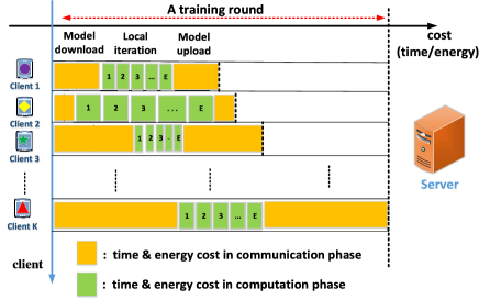
Figure 1: A typical federated learning round with $K$ sampled clients and $E$ steps of local iterations.

As illustrated in Fig. 1, we consider the number of participating clients (${K}$) and the number of local iterations (${E}$) in each FL round as our control variables. A similar methodology can be applied to analyze problems with other control variables as well. We analyze, for the first time, how to design adaptive FL that optimally chooses $K$ and $E$ to minimize the total cost while ensuring convergence. Our main contributions are as follows:

• Optimization Algorithm: We establish the analytical relationship between the total cost, control variables, and convergence upper bound for strongly convex objective functions, based on which an optimization problem for total cost minimization is formulated and analyzed. We propose a sampling-based algorithm to learn the unknown parameters in the convergence bound with marginal estimation overhead. We show that our optimization problem is biconvex with respect to $K$ and $E$, and develop efficient ways to solve it based on closed-form expressions.

• Theoretical Properties: We theoretically obtain important properties that effectively identify the design principles for different optimization goals. Notably, the choice of $K$ leads to an interesting trade-off between learning time reduction and energy saving, with a large $K$ favoring the former while a small $K$ benefiting the later. Nevertheless, we show that a relatively low device participation rate does not severely slow down the learning. For the choice of $E$, we show that neither a too small or too large $E$ is good for cost-effectiveness. The optimal value of $E$ also depends on the relationship between computation and communication costs.

• Simulation and Experimentation: We evaluate our theoretical results with real datasets, both in a simulated environment and on a hardware prototype with $20$ Raspberry Pi devices. Experimental results verify our design principles and derived properties of $K$ and $E$. They also demonstrate that our proposed optimization algorithm provides near-optimal solution for both real and synthetic datasets with non-i.i.d. data distributions. Particularly, we highlight that our approach works well with both convex non-convex machine learning models empirically.

II Related Work

FL was first proposed in [2], which demonstrated FL’s effectiveness of collaboratively learning a model without collecting users’ data. Compared to distributed learning in data centers, FL needs to address several unique challenges, including non-i.i.d. and unbalanced data, limited communication bandwidth, and limited device availability (partial participation) [1, 5]. It was suggested that FL algorithms should operate synchronously due to its composability with other techniques such as secure aggregation protocols [15], differential privacy [16], and model compression [17]. Hence, we consider synchronous FL in this paper with all the aforementioned characteristics.

The de facto FL algorithm is federated averaging (FedAvg), which performs multiple local iterations in parallel on a subset of devices in each round. A system-level FL framework was presented in [8], which demonstrates the empirical success of FedAvg in mobile devices using TensorFlow [18]. Recently, a convergence bound of FedAvg was established in [11]. Other related distributed optimization algorithms are mostly for i.i.d. datasets [19, 20, 21] and full client participation [22, 9, 23], which do not capture the essence of on-device FL. Some extensions of FedAvg considered aspects such as adding a proximal term [10] and using accelerated gradient descent methods [24]. These works did not consider optimization for cost/resource efficiency.

Literature in FL cost optimization mainly focused on learning time and on-device energy consumption. The optimization of learning time was studied in [25, 26, 27, 28, 29, 30, 31, 32], and joint optimization for learning time and energy consumption was considered in [33, 34, 35]. These works considered cost-aware client scheduling [25, 26, 27, 28], task offloading[36] and resource (e.g., transmission power, communication bandwidth, and CPU frequency) allocation [29, 30, 12, 33, 34, 35] for pre-specified (i.e., non-optimized) design parameters ($K$ and $E$ in our case) of the FL algorithm.

The optimization of a single design parameter $E$ or the amount of information exchange, in general, was studied in [13, 14, 12, 31, 37, 38], most of which assume full client participation and can be infeasible for large-scale on-device FL. A very recent work in [39] considered the optimization of both $E$ and client selection for additive per-client costs. However, the cost related to learning time in our problem is non-additive on a per-client basis, because different clients perform local model updates in parallel. In addition, the convergence bound used in [39] (and also [12]) is for a primal-dual optimization algorithm, which is different from the commonly used FedAvg algorithm and does not reflect the impact of key FL characteristics such as partial client participation. The challenge in optimizing both $K$ and $E$ for cost minimization of FedAvg that takes into account all the aforementioned FL characteristics, which also distinguishes our work from the above, is the need to analytically connect the total cost with multiple control variables as well as with the convergence rate.

In addition, most existing work on FL are based on simulations, whereas we implement our algorithm in an actual hardware prototype with resource-constrained devices.

Roadmap: We present the system model and problem formulation in Section III. In Section IV, we analyze the cost minimization problem and present an algorithm to solve it. We provide theoretical analysis on the solution properties in Section V. Experimentation results are given in Section VI and the conclusion is presented in Section VII.

III System Model

We start by summarizing the basics of FL and its de facto algorithm FedAvg. Then, we present the cost model for a given FL task, and introduce our optimization problem formulation.

III-A Federated Learning

Consider a scenario with a large population of mobile clients that have data for training a machine learning model. Due to data privacy and bandwidth limitation concerns, it is not desirable for clients to disclose and send their raw data to a high-performance data center. FL is a decentralized learning framework that aims to resolve this problem. Mathematically, FL is the following distributed optimization problem:

$$\min_{\mathbf{w}}F\left(\mathbf{w}\right):=\sum\nolimits_{k=1}^{N}{p_{k}}{F_{k}}\left(\mathbf{w}\right)$$ (1)

where the objective $F\left(\mathbf{w}\right)$ is also known as the global loss function, $\mathbf{w}$ is the model parameter vector, $N$ is the total number of devices, and $p_{k}$ is the weight of the $k$-th device such that $\sum\nolimits_{k=1}^{N}p_{k}=1$. Suppose the $k$-th device has $n_{k}$ training data samples ($\mathbf{x}_{k,1},\cdots,\mathbf{x}_{k,n_{k}}$), and the total number of training data samples across $N$ devices is $n:=\sum\nolimits_{k\!=\!1}^{N}n_{k}$, then we have $p_{k}=\frac{n_{k}}{n}$. The local loss function of client $k$ is

$${F_{k}}\left(\mathbf{w}\right):=\frac{1}{{{n_{k}}}}\sum\limits_{j=1}^{n_{k}}{{f}\left(\mathbf{w};\mathbf{x}_{k,j}\right)},$$ (2)

where $f(\cdot)$ represents a per-sample loss function, e.g., mean square error and cross entropy applied to the output of a model with parameter $\mathbf{w}$ and input data sample $\mathbf{x}_{k,j}$ [13].

FedAvg (Algorithm 1) was proposed in [2] to solve (1). In each round $r$, a subset of randomly selected clients $\mathcal{K}^{(r)}$ run $E$ steps of stochastic gradient decent (SGD) on (2) in parallel, where $\mathcal{K}^{(r)}\subseteq\{1,2,...,N\}$. Then, the updated model parameters of these $\left|\mathcal{K}^{(r)}\right|$ clients are sent to and aggregated by the server. This process repeats for many rounds until the global loss converges. Let $R$ be the total number of rounds, then the total number of iterations for each device is $ER$.

While FL has demonstrated its effectiveness in many application scenarios, practitioners also need to take into account the cost that is incurred for completing a given task.

Input: $K$, $E$, precision $\epsilon$, initial model $\mathbf{w_{0}}$

Output: Final model parameter $\mathbf{w}_{R}$

1 for $r=0,1,2,...,R$ do

       Server randomly selects a subset of clients $\mathcal{K}^{(r)}$ and sends the current global model parameter $\mathbf{w}_{r}$ to the selected clients;

        // Communication

2      

      Each selected client $k\in\mathcal{K}^{(r)}$ in parallel updates $\mathbf{w}_{r}$ by running $E$ steps of SGD on (2) to compute a new model $\mathbf{w}_{r}^{(k)}$;

        // Computation

3      

      Each selected client $k\in\mathcal{K}^{(r)}$ sends back the updated model $\mathbf{w}_{r}^{(k)}$ to the server;

        // Communication

4      

      Server computes the new global model parameter $\mathbf{w}_{r+1}\leftarrow\frac{\sum_{k\in\mathcal{K}^{(r)}}p_{k}\mathbf{w}_{r}^{(k)}}{\sum_{k\in\mathcal{K}^{(r)}}p_{k}}$;

        // Aggregation

5      

6      $r\leftarrow r+1$;

Algorithm 1 Federated Learning Algorithm

III-B Cost Analysis of Federated Learning

The total cost of FL, according to Algorithm 1, involves learning time and energy consumption, both of which are consumed during local computation (Line 1) and global communication (Lines 1 and 1) in each round. Before presenting each cost model, we first give the system assumptions.

System assumptions: Similar to existing works [2, 11, 10], we sample $K$ clients in each round $r$ (i.e., $K:=\left|\mathcal{K}^{(r)}\right|$) where the sampling is uniform (without replacement) out of all $N$ clients. We assume the communication and computation cost for a particular device in each round is the same, but varies among devices due to system heterogeneity. We do not consider the cost for model aggregation in Line 1, because it only needs to compute the average that is much less complex than local model updates.

III-B1 Time Cost

For general heterogeneous systems, each client can have different communication and computation capabilities (see Fig. 1). Let $t_{k}$ denote the per-round time for client $k$ to complete computation and communication. We have

$$t_{k}=t_{k,p}E+t_{k,m}\ \forall k\in\{1,\ldots,N\},$$ (3)

where $t_{k,p}$ is the computation time for client $k$ to perform one local iteration, and $t_{k,m}$ is the per-round communication time for a client to upload/download the model parameter.

Because the clients compute and communicate in parallel, for each round $r$, the per-round time $t^{(r)}$ depends on the slowest participating client (also known as straggler). Hence,

$$t^{(r)}=\max_{k\in\mathcal{K}^{(r)}}\left\{t_{k}\right\}.$$ (4)

Therefore, the total learning time $t_{\textnormal{tot}}$ after $R$ rounds is

$$t_{\textnormal{tot}}(K,E,R)=\sum\nolimits_{r=1}^{R}\max_{k\in\mathcal{K}^{(r)}}\left\{t_{k}\right\}.$$ (5)

III-B2 Energy Cost

Similarly, by denoting $e_{k}$ as the per-round energy cost for client $k$ to complete the computation and communication, we have

$$e_{k}=e_{k,p}E+e_{k,m},$$ (6)

where $e_{k,p}$ and $e_{k,m}$ are respectively the energy costs for client $k$ to perform a local iteration and a round of communication.

Unlike the straggling effect in time cost (4), the energy cost $e^{(r)}$ in each round $r$ depends on the sum energy consumption of the selected clients $\mathcal{K}^{(r)}$. Therefore, the total energy cost $e_{\textnormal{tot}}$ after $R$ rounds can be expressed as

$$e_{\textnormal{tot}}(K,E,R)=\sum\nolimits_{r=1}^{R}\sum\nolimits_{k\in\mathcal{K}^{(r)}}e_{k}.$$ (7)

III-C Problem Formulation

Considering the difference of the two cost metrics, the optimal solutions of $E$, $K$ and $R$ generally do not achieve the common goal for minimizing both $t_{\textnormal{tot}}$ and $e_{\textnormal{tot}}$. To strike the balance of learning time and energy consumption, we introduce a weight $\gamma\in\left[0,1\right]$ and optimize the balanced cost function in the following form:

$$C_{\textnormal{tot}}(K,E,R)=\left(1-\gamma\right)t_{\textnormal{tot}}(K,E,R)+\gamma e_{\textnormal{tot}}(K,E,R),$$ (8)

where $1-\gamma$ and $\gamma$ can be interpreted as the normalized price of the two costs, i.e., how much monetary cost for one unit of time and one unit of energy, respectively. The value of $\gamma$ can be adjusted for different preferences. For example, we can set $\gamma=0$ when all clients are plugged in and energy consumption is not a major concern, whereas $\gamma=1$ when devices are solar-based sensors where saving the devices’ energy is the priority.

Our goal is to minimize the expected total cost while ensuring convergence, which translates into this problem:

$$\begin{array}[]{cl}\!\!\!\!\!\!\!\!\textbf{P1:}\quad\quad\min_{E,K,R}&\mathbb{E}[C_{\textnormal{tot}}(E,K,R)]\\ \quad\quad\text{ s.t. }&\mathbb{E}[F(\mathbf{w}_{R})]-F^{*}\leq\epsilon,\\ &K,E,R\in\mathbb{Z}^{+},\ \text{and}\ \ 1\leq K\leq N.\end{array}$$ (9)

where $\mathbb{E}[F(\mathbf{w}_{R})]$ is the expected loss after $R$ rounds, $F^{*}$ is the (true and unknown) minimum value of $F$, and $\epsilon$ is the desired precision. We note that the expectation in P1 is due to the randomness of SGD and client sampling in each round.

Solving P1 is challenging in two aspects. First, it is difficult to find an exact analytical expression to relate $E$, $K$ and $R$ with $C_{\textnormal{tot}}$, especially due to the non-linear maximum function in $t_{\textnormal{tot}}$. Second, it is generally impossible to obtain an exact analytical relationship to connect $E$, $K$ and $R$ with the convergence constraint. In the following section, we propose an algorithm that approximately solves P1, which we later show with extensive experiments that the proposed solution can achieve a near-optimal performance of P1.

IV Cost-Effective Optimization Algorithm

This section shows how to approximately solve P1. We first formulate an alternative problem that includes an approximate analytical relationship between the expected cost $\mathbb{E}[C_{\textnormal{tot}}]$, the convergence constraint, and the control variables $E$, $K$ and $R$. Then, we show that this new optimization problem can be efficiently solved after estimating unknown parameters associated with the convergence bound, and we propose a sampling-based algorithm to learn these unknown parameters.

IV-A Approximate Solution to P1

IV-A1 Analytical Expression of $\mathbb{E}[e_{\textnormal{tot}}]$

We first analytically establish the expected energy cost $\mathbb{E}[e_{\textnormal{tot}}]$ with $K$ and $E$.

Lemma 1.

The expectation of $e_{\textnormal{tot}}$ in (7) can be expressed as

$$\mathbb{E}[e_{\textnormal{tot}}(K,E,R)]=K\left(e_{p}E+e_{m}\right)R,$$ (10)

where $e_{p}:=\frac{\sum_{k=1}^{N}e_{k,p}}{N}$ and $e_{m}:=\frac{\sum_{k=1}^{N}e_{k,m}}{N}$ denote the average per-device energy consumption for one local iteration and one round of communication, respectively.

Proof.

Since all devices are sampled uniformly at random in each round, for $R$ rounds, each device will be sampled in $\frac{KR}{N}$ rounds in expectation. Given that each device $k$ consumes $e_{k,p}E+e_{k,m}$ energy in each round as shown in (6), summing up $\frac{KR}{N}\left(e_{k,p}E+e_{k,m}\right)$ over all $N$ clients leads to (10). ∎

IV-A2 Analytical Expression of $\mathbb{E}[t_{\textnormal{tot}}]$

Next, we show how to tackle the straggling effect to establish the expected time cost $\mathbb{E}[t_{\textnormal{tot}}]$ with the control variables. Without loss of generality, we reorder $\{t_{k}:\forall k\in\{1,2,...,N\}\}$, such that

$$t_{1}\leq t_{2}\leq\ldots\leq t_{k}\leq\ldots\leq t_{N}.$$ (11)

Lemma 2.

With the reordered $t_{k}$ as in (11), the expectation of $t_{\textnormal{tot}}$ in (5) can be expressed as

$$\begin{array}[]{c}\mathbb{E}[t_{\textnormal{tot}}(K,E,R)]=\frac{\sum\nolimits_{i=K}^{N}{C_{i-1}^{K-1}t_{i}}}{C_{N}^{K}}R.\end{array}$$ (12)

Proof.

We omit the full proof due to page limitation. The idea is to show that the expectation of the per-round time in (4) is

$$\begin{array}[]{c}\mathbb{E}[t^{(r)}]=\frac{1}{C_{N}^{K}}\sum\nolimits_{i=K}^{N}{C_{i-1}^{K-1}t_{i}}.\end{array}$$ (13)

We first use the recursive property of $C_{m}^{n}\!+C_{m}^{n-1}\!=\!C_{m+1}^{n}$ to show that the number of total combinations for choosing $K$ out of $N$ devices ${C_{N}^{K}}$ can be extended as ${C_{N}^{K}}=\sum\nolimits_{i=K}^{N}{C_{i-1}^{K-1}}$. Then, each combination (e.g., $C_{N-1}^{K-1}$) corresponds to the number of a certain device (e.g., $N$) being the slowest one (e.g., $t_{N}$). Since all devices are sampled uniformly at random, taking the expectation of all combinations gives (13). ∎

IV-A3 Analytical Relationship Between $\mathbb{E}[C_{\textnormal{tot}}]$ and Convergence

Based on $\mathbb{E}[e_{\textnormal{tot}}]$ in (10) and $\mathbb{E}[{t_{\textnormal{tot}}}]$ in (12), the objective function $\mathbb{E}[{C_{\textnormal{tot}}}]$ in P1 can be expressed as

$$\begin{array}[]{c}\mathbb{E}[{C_{\textnormal{tot}}}]\!=\!\left(\frac{\left(1-\!\gamma\right)\sum\nolimits_{i=K}^{N}{C_{i-1}^{K-1}t_{i}}}{C_{N}^{K}}\!+\!\gamma K\left(e_{p}E+e_{m}\right)\right)R.\end{array}$$ (14)

To connect $\mathbb{E}[{C_{\textnormal{tot}}}]$ with the $\epsilon$-convergence constraint in (9), we utilize the convergence result [11]:

$$\begin{array}[]{c}\mathbb{E}[F(\mathbf{w}_{R})]-F^{*}\leq\frac{1}{ER}\left(A_{0}+B_{0}\left(1+\frac{N-K}{K(N-1)}\right)E^{2}\right),\end{array}$$ (15)

where $A_{0}$ and $B_{0}$ are loss function related constants characterizing the statistical heterogeneity of non-i.i.d. data. By letting the upper bound satisfy the convergence constraint, and using (14) and Lemmas 1 and 2, we approximate P1 as

$$\begin{array}[]{cl}\!\!\!\!\!\!\textbf{P2:}\ \min_{E,K,R}&\!\!\!\left(\frac{\left(1-\!\gamma\right)\sum\nolimits_{i=K}^{N}{C_{i-1}^{K-1}t_{i}}}{C_{N}^{K}}\!+\!\gamma K\left(e_{p}E+e_{m}\right)\right)R\\ \quad\text{ s.t. }&\!\!\!\frac{1}{ER}\left(A_{0}+B_{0}\left(1+\frac{N-K}{K(N-1)}\right)E^{2}\right)\leq\epsilon\\ &K,E,R\in\mathbb{Z}^{+},\ \text{and}\ \ 1\leq K\leq N.\end{array}$$ (16)

Combining with (15), we can see that P2 is more constrained than P1, i.e., any feasible solution of P2 is also feasible for P1.

Problem P2, however, is still hard to optimize because it requires to compute various combinatorial numbers with respect to $K$. Moreover, even for a fixed value of $K$, the combinatorial term is based on the reordering of $t_{k}$ in (3), which is uncertain as the order of $t_{k}$ changes with $E$. For analytical tractability, we further approximate P2 as follows.

IV-A4 Approximate Optimization Problem of P2

To address the complexity involved with computing the combinatorial term in (14), similar to how we derive (10), we define an approximation of $\mathbb{E}[t_{\textnormal{tot}}]$ as

$$\tilde{\mathbb{E}}[t_{\textnormal{tot}}(E,R)]:=\left(t_{p}E+t_{m}\right)R,$$ (17)

where $t_{p}\!:=\!\frac{\sum_{k=1}^{N}t_{k,p}}{N}$ and $t_{m}\!:=\!\frac{\sum_{k=1}^{N}t_{k,m}}{N}$ are the average per-device time cost for one local iteration and one round of communication, respectively. The approximation $\tilde{\mathbb{E}}[t_{\textnormal{tot}}]$ is equivalent to $\mathbb{E}[t_{\textnormal{tot}}]$ in the following two cases.

Case 1: For homogeneous systems, where $t_{p}=t_{k,p}$ and $t_{m}=t_{k,m},\forall k\in\{1,\ldots,N\}$, we have

$$\begin{array}[]{cl}\mathbb{E}[{t_{\textnormal{tot}}}(K,E,R)]&=\left(t_{p}E+t_{m}\right)\frac{\sum\nolimits_{i=K}^{N}{C_{i-1}^{K-1}}}{C_{N}^{K}}R\\ &=\left(t_{p}E+t_{m}\right)R\\ &=\tilde{\mathbb{E}}[t_{\textnormal{tot}}(E,R)].\end{array}$$

Case 2: For heterogeneous systems with $K\!=\!1$, we have

$$\begin{array}[]{cl}\mathbb{E}[{t_{\textnormal{tot}}}(K=1,E,R)]&=\left(\frac{t_{1}+t_{2}\ldots+t_{N}}{N}\right)R\\ &=\left(\frac{\sum_{k=1}^{N}t_{k,p}E+\sum_{k=1}^{N}t_{k,m}}{N}\right)R\\ &=\left(t_{p}E+t_{m}\right)R\\ &=\tilde{\mathbb{E}}[t_{\textnormal{tot}}(E,R)].\end{array}$$

Based on the approximation $\tilde{\mathbb{E}}[t_{\textnormal{tot}}(E,R)]$ in (17), we formulate an approximate objective function of P2 as

$$\tilde{\mathbb{E}}[C_{\textnormal{tot}}(K,E,R)]=\left(1-\gamma\right)\tilde{\mathbb{E}}[t_{\textnormal{tot}}(E,R)]+\gamma\mathbb{E}[e_{\textnormal{tot}}(K,E,R)].$$ (18)

Now, we relax $K$, $E$ and $R$ as continuous variables for theoretical analysis, which are rounded back to integer variables later. For the relaxed problem, if any feasible solution $E^{\prime},K^{\prime}$, and $R^{\prime}$ satisfies the $\epsilon$-constraint in P2 with inequality, we can always decrease this $R^{\prime}$ to some $R^{\prime\prime}<R^{\prime}$ which satisfies the constraint with equality but reduces the objective function value. Hence, for optimal $R$, the $\epsilon$-constraint is always satisfied with equality, and we can obtain $R$ from this equality as

$$\begin{array}[]{c}R=\frac{1}{\epsilon E}\left(A_{0}+B_{0}\left(1+\frac{N-K}{K(N-1)}\right)E^{2}\right).\end{array}$$ (19)

By using $\tilde{\mathbb{E}}[C_{\textnormal{tot}}]$ to approximate $\mathbb{E}[C_{\textnormal{tot}}]$ and substituting (19) into its expression, we obtain

$$\begin{array}[]{cl}\!\!\!\!\!\!\!\!\!\!\!\!\!\!\!\textbf{P3:}\\ \min_{E,K}&\!\!\!\!\!\frac{\left(\left(1-\gamma\right)\left(t_{p}E+t_{m}\right)+\gamma K\left(e_{p}E+e_{m}\right)\right)\cdot\left(\!A_{0}+B_{0}\left(\!1+\frac{N-K}{K(N-1)}\!\right)E^{2}\right)}{\epsilon E}\\[6.0pt] \!\!\!\!\!\quad\text{s.t.}&\!\!\!{E}\geq 1,\ \text{and}\ \ 1\leq K\leq N,\end{array}$$ (20)

where we note that the objective function of P3 is equal to $\tilde{\mathbb{E}}[C_{\textnormal{tot}}]$. P3 is an approximation of P2 due to the use of $\tilde{\mathbb{E}}[C_{\textnormal{tot}}]$ to approximate the original objective $\mathbb{E}[C_{\textnormal{tot}}]$.

In the following, we solve P3 as an approximation of the original P1. Our empirical results in Section VI demonstrate that the solution obtained from solving P3 achieves near-optimal performance of the original problem P1. For ease of analysis, we incorporate $\epsilon$ in the constants $A_{0}$ and $B_{0}$ next.

IV-B Solving the Approximate Optimization Problem P3

In this subsection, we first characterize some properties of the optimization problem P3. Then, we propose a sampling-based algorithm to learn the problem-related unknown parameters $A_{0}$ and $B_{0}$, based on which the solution $K^{*}$ and $E^{*}$ (of P3) can be efficiently computed. The overall algorithm for obtaining $K^{*}$ and $E^{*}$ is given in Algorithm 2.

Input: $N$, $\gamma$, $t_{p}$, $t_{m}$, $e_{p}$, $e_{m}$, loss $F_{a}$ and $F_{b}$, $\mathbf{w}_{0}$, number of sampled pairs $M$, stopping condition $\epsilon_{0}$

Output: $K^{*}$ and $E^{*}$

1

2for $i=1,2,\ldots,M$  do

3       Empirically choose $(K_{i}$, $E_{i})$ and run Algorithm 1;

4      Record $R_{i,a}$ and $R_{i,b}$ when $F_{a}$ and $F_{b}$ are reached;

5Calculate average $\frac{A_{0}}{B_{0}}$ using (25);

6Choose a feasible $z_{0}\leftarrow\left(K_{0},E_{0}\right)$ and set $j\leftarrow 0$;

7while $\|z_{j}-z_{j-1}\|>\epsilon_{0}$ do

8       Substitute $E_{j}$, $\frac{A_{0}}{B_{0}}$, $N$, $\gamma$, $t_{p}$, $t_{m}$, $e_{p}$, $e_{m}$ into (21) and derive $K^{\prime}$;

9      $K_{j+1}\leftarrow\arg\min_{K\in[1,N]}|K-K^{\prime}|$;

10      Substitute $K_{j+1}$, $\frac{A_{0}}{B_{0}}$, $N$, $\gamma$, $t_{p}$, $t_{m}$, $e_{p}$, $e_{m}$ into (22) and derive $E^{\prime}$;

11      $E_{j+1}\leftarrow\arg\min_{E\geq 1}|E-E^{\prime}|$;

12      $z_{j+1}\leftarrow\left(K_{j+1},E_{j+1}\right)$ and $j\leftarrow j+1$;

13Substitute four rounding combinations of $\left(\left\lceil{K_{j}}\right\rceil,\left\lceil{E_{j}}\right\rceil\right)$, $\left(\left\lceil{K_{j}}\right\rceil,\left\lfloor{E_{j}}\right\rfloor\right)$, $\left(\left\lfloor{K_{j}}\right\rfloor,\left\lceil{E_{j}}\right\rceil\right)$, and $\left(\left\lfloor{K_{j}}\right\rfloor,\left\lfloor{E_{j}}\right\rfloor\right)$ into the objective function of P3, and set the pair with the minimum value as $\left(K^{*},E^{*}\right)$

14return $\left(K^{*},E^{*}\right)$

Algorithm 2 Cost-effective design of $K$ and $E$

IV-B1 Characterizing P3

The objective function of P3 is non-convex because the determinant of its Hessian $\frac{\partial^{2}\tilde{\mathbb{E}}[C_{\textnormal{tot}}]}{\partial^{2}K}\frac{\partial^{2}\tilde{\mathbb{E}}[C_{\textnormal{tot}}]}{\partial^{2}E}-(\frac{\partial^{2}\tilde{\mathbb{E}}[C_{\textnormal{tot}}]}{\partial K\partial E})^{2}$ is not always non-negative in the feasible set. However, the problem is biconvex [40].

Theorem 1.

Problem P3 is strictly biconvex.

Proof.

For any $E\geq 1$, we have

$$\frac{\partial^{2}\tilde{\mathbb{E}}[C_{\textnormal{tot}}]}{\partial^{2}K}=\frac{2(1-\gamma)B_{0}N\left(t_{p}E^{2}+t_{m}E\right)}{(N-1)K^{3}}>0.$$

Similarly, for any $1\leq K\leq N$, we have

$$\begin{array}[]{cl}\dfrac{\partial^{2}\tilde{\mathbb{E}}[C_{\textnormal{tot}}]}{\partial^{2}E}\!\!\!\!\!\!&=2\left(\left(1\!-\!\gamma\right)t_{p}+\gamma Ke_{p}\right)B_{0}\left(1+\frac{N-K}{K(N-1)}\right)\\ &\ \ +\dfrac{2A_{0}\left[(1\!-\!\gamma)t_{m}+\gamma Ke_{m}\right]}{E^{3}}>0\end{array}$$

Since the domain of $K$ and $E$ is convex as well, we conclude that P3 is strictly biconvex. ∎

The biconvex property allows many efficient algorithms, such as Alternate Convex Search (ACS) approach, to a achieve a guaranteed local optima[40]. Nevertheless, by analyzing the stationary point of $\frac{\partial\tilde{\mathbb{E}}[C_{\textnormal{tot}}]}{\partial K}=0$ and $\frac{\partial\tilde{\mathbb{E}}[C_{\textnormal{tot}}]}{\partial E}\!=\!0$, we show that the optimal solution can be found more efficiently. This is because from $\frac{\partial\tilde{\mathbb{E}}[C_{\textnormal{tot}}]}{\partial K}\!=\!0$ we have $K$ in closed-form of $E$ as

$$\begin{array}[]{cl}K=\sqrt{\frac{(1-\gamma)B_{0}N\left(t_{p}E^{3}+t_{m}E^{2}\right)}{\gamma\left[B_{0}(N-2)E^{2}+A_{0}(N-1)\right](e_{p}E+{e_{m}})}}.\end{array}$$ (21)

By letting $\frac{\partial\tilde{\mathbb{E}}[C_{\textnormal{tot}}]}{\partial E}=0$, we derive the cubic equation of $E$ as

$$\begin{array}[]{cl}\frac{2\left(1-\gamma\right)t_{p}+\gamma Ke_{p}}{2\left(1-\gamma\right)t_{m}+\gamma Ke_{m}}E^{3}+E^{2}-{\frac{A_{0}}{B_{0}\left(1+\frac{N-K}{K(N-1)}\right)}}\!=\!0,\end{array}$$ (22)

which can be analytically solved in closed-form of $K$ via Cardano formula [41]. Therefore, for any fixed value of $K$, due to biconvexity (Theorem 1), we have a unique real solution of $E$ from (22) in closed form. Then, with ACS method we iteratively calculate (21) and (22) which keeps decreasing the objective function until we achieve the converged $K^{\ast}$ and $E^{\ast}$. This optimization process corresponds to Lines 2–2 of Algorithm 2, where Lines 2 and 2 ensure that the solution is taken within the feasibility region, and Line 2 rounds the continuous values of $K$ and $E$ to integer values.

IV-B2 Estimation of Parameters $\frac{A_{0}}{B_{0}}$

Equations (21) and (22) include unknown parameters $A_{0}$ and $B_{0}$, which can only be determined during the learning process. In fact, $K$ in (21) and $E$ in (22) only depend on the value of $\frac{A_{0}}{B_{0}}$. In the following, we propose a sampling-based algorithm to estimate $\frac{A_{0}}{B_{0}}$, and show that the overhead for estimation is marginal.

The basic idea is to sample different combinations of $\left(K,E\right)$ and use the upper bound in (15) to approximate $F(\mathbf{w}_{R})\!-\!F^{*}$. Specifically, we empirically sample a pair $\left(K_{i},E_{i}\right)$ and run Algorithm 1 with an initial model $\mathbf{w}_{0}\!=\!\mathbf{0}$ until it reaches two pre-defined global losses $F_{a}:=F(\mathbf{w}_{R_{i,a}})$ and $F_{b}:=F(\mathbf{w}_{R_{i,b}})$ ($F_{b}<F_{a}$), where $R_{i,a}$ and ${R_{i,b}}$ are the executed round numbers for reaching losses $F_{a}$ and $F_{b}$. The pre-defined losses $F_{a}$ and $F_{b}$ can be set to a relatively high value, to keep a small estimation overhead, but they cannot be too high either as it would cause low estimation accuracy. Then, we have

$$\begin{cases}R_{i,a}\approx d+\frac{A_{0}+B_{0}\left(1+\frac{N-K_{i}}{K_{i}(N-1)}\right)E_{i}^{2}}{E_{i}\left(F_{a}-F^{*}\right)},\\ {R_{i,b}}\approx d+\frac{A_{0}+B_{0}\left(1+\frac{N-K_{i}}{K_{i}(N-1)}\right)E_{i}^{2}}{E_{i}\left(F_{b}-F^{*}\right)}.\end{cases}$$ (23)

from (15), where $d$ captures a constant error of using the upper bound to approximate $F(\mathbf{w}_{R})\!-\!F^{*}$. Based on (23), we have

$$\begin{array}[]{c}{R_{i,b}}-R_{i,a}\approx\frac{\Delta}{E_{i}}\left({A_{0}\!+\!B_{0}\left(1\!+\!\frac{N-K_{i}}{K_{i}(N\!-\!1)}\right)\!E_{i}^{2}}\right),\end{array}$$ (24)

where $\Delta:=\frac{1}{F_{b}\!-\!F^{*}}\!-\!\frac{1}{F_{a}\!-\!F^{*}}$. Similarly, sampling another pair of ($K_{j}$, $E_{j}$) and performing the above process gives us another executed round numbers $R_{j,a}$ and $R_{j,b}$. Thus, we have

$$\begin{array}[]{c}\frac{E_{i}\left(R_{i,b}-R_{i,a}\right)}{E_{j}\left(R_{j,b}-R_{j,a}\right)}\approx\frac{{A_{0}+B_{0}\left(1+\frac{N-K_{i}}{K_{i}(N-1)}\right)E_{i}^{2}}}{{A_{0}+B_{0}\left(1+\frac{N-K_{j}}{K_{j}(N-1)}\right)E_{j}^{2}}}.\end{array}$$ (25)

We can obtain $\frac{A_{0}}{B_{0}}$ from (25) (note that the variables except for $\frac{A_{0}}{B_{0}}$ are known). In practice, we may sample several different pairs of $\left(K_{i},E_{i}\right)$ to obtain an averaged estimation of $\frac{A_{0}}{B_{0}}$. This estimation process is given in Lines 2–2 of Algorithm 2.

Estimation overhead: The main overhead for estimation comes from the additional iterations for the estimation of $\frac{A_{0}}{B_{0}}$.

For $M$ sampling pairs, the total number of iterations used for estimation is $\sum_{i=1}^{M}R_{i,b}E_{i}$, where $R_{i,b}$ is the number of rounds for sampling pair ($K_{i}$, $E_{i}$) to reach $F_{b}$. If the target loss is $F_{R}$ with the required number of rounds $R$, then according to (15), the overhead ratio can be written as

$$\begin{array}[]{c}\frac{\sum_{i=1}^{M}R_{i,b}E_{i}}{RE^{*}}\approx\frac{\sum_{i=1}^{M}R_{i,b}E_{i}\left({F_{R}-F^{\ast}}\right)}{A_{0}+B_{0}\left(1+\frac{N-K^{\ast}}{K^{\ast}(N-1)}\right)\cdot({E^{\ast}})^{2}},\end{array}$$ (26)

where $K^{*}$ and $E^{*}$ are obtained from Algorithm 2. For a high precision with $F_{R}-F^{*}\rightarrow 0$, the overhead ratio is marginal.

V Solution Property for Cost Minimization

We theoretically analyze the solution properties for different metric preferences, which not only provide insightful design principles but also give alternative ways of solving P3 to more efficiently. Our empirical results show that these properties derived for P3 are still valid for the original P1. In the following, we discuss the properties for $\gamma=0$ and $\gamma=1$, respectively. For ease of presentation, we consider continuous $K$, $K^{*}$, $E$, and $E^{*}$ (i.e., before rounding) in this section.

V-A Properties for Minimizing $\tilde{\mathbb{E}}[C_{\textnormal{tot}}]$ when $\gamma=0$

When the design goal is to minimize learning time ($\gamma=0$), the objective of P3 can be rewritten as

$$\begin{array}[]{c}\min_{E,K}\ \left(\frac{t_{m}}{E}+t_{p}\right)\cdot\left(A_{0}+B_{0}\left(1+\frac{N-K}{K(N-1)}\right)E^{2}\right)\end{array}$$ (27)

We present the following insightful results to characterize the properties of $E^{*}$ and $K^{*}$.

Theorem 2.

When $\gamma=0$, $\tilde{\mathbb{E}}[C_{\textnormal{tot}}]$ is a strictly decreasing function in $K$ for any given $E$, hence $K^{*}=N$.

Proof.

The proof is straightforward, as we are able to show for any $E$, $\frac{\partial\tilde{\mathbb{E}}[C_{\textnormal{tot}}]}{\partial K}<0$. Since $K\leq N$, we have $K^{*}=N$. The same result can also be obtained by letting $\gamma\rightarrow 0$ in (21). ∎

Remark: In practical FL applications, $N$ can be very large, and thus, full participation ($K\!=\!N$) is usually intractable. However, since the objective function in (27) is strictly convex and decreasing with $K$, as $K$ increases, the marginal learning time decrease becomes smaller as well. Therefore, when $N$ is very large, sampling a small portion of devices can achieve a relative good learning time. Our later real-data experiment shows that sampling $K\!=\!20$ out of $N\!=\!100$ devices achieves a similar performance as sampling all devices.

Based on the above finding, it is important to analyze the property of $E$ when $K$ is chosen sub-optimally. In line with this, we present the following two corollaries.

Corollary 1.

When $\gamma=0$, for any fixed value of $K$, as $E$ increases, $\tilde{\mathbb{E}}[C_{\textnormal{tot}}]$ first decreases and then increases.

Proof.

Taking the first order derivative of $\tilde{\mathbb{E}}[C_{\textnormal{tot}}]$ over $E$,

$$\begin{array}[]{c}\frac{\partial\tilde{\mathbb{E}}[C_{\textnormal{tot}}]}{\partial E}=B_{0}\left(2t_{p}E+t_{m}\right)\left(1+\frac{N-K}{K(N-1)}\right)-\frac{t_{m}A_{0}}{E^{2}}.\end{array}$$ (28)

Since $0\leq\frac{N-K}{K(N-1)}\leq 1$ for any feasible $K$, (28) is negative when $E$ is small and positive when $E$ is large. ∎

Corollary 1 shows that for any given $K$, $E$ should not be set too small nor too large for saving learning time.

Corollary 2.

When $\gamma=0$, for any fixed value of $K$, $E^{*}$ increases as $\frac{t_{m}}{t_{p}}$ increases.

We omit the proof of Corollary 2 due to page limitation. Intuitively, Corollary 2 says that for any given $K$, when $t_{m}$ increases or $t_{p}$ decreases, the optimal strategy to reduce learning time is to perform more steps of iterations (i.e., increase $E$) before aggregation, which matches the empirical observations for communication efficiency in [2, 19, 20].

V-B Properties for Minimizing $\tilde{\mathbb{E}}[C_{\textnormal{tot}}]$ when $\gamma=1$

When the design goal is to minimize energy consumption ($\gamma=1$), the objective of P3 can be rewritten as

$$\begin{array}[]{c}\min_{E,K}\left(\frac{e_{m}K}{E}\!+\!e_{p}K\right)\left(A_{0}\!+\!B_{0}\left(1\!+\frac{N-K}{K(N\!-\!1)}\right)\!E^{2}\right).\end{array}$$ (29)

Besides the different metrics of $e_{m}$ and $e_{p}$, the key difference between (27) and (29) is the multiplication of $K$. Therefore, the main difference between $\gamma=1$ and $\gamma=0$ is in the properties related to $K$, whereas the properties related to $E$ remain similar, which we show in the following.

Theorem 3.

When $\gamma=1$, $\tilde{\mathbb{E}}[C_{\textnormal{tot}}]$ is a strictly increasing function in $K$ for any given $E$, hence $K^{*}=1$.

Proof.

It is easy to show that $\frac{\partial\tilde{\mathbb{E}}[C_{\textnormal{tot}}]}{\partial K}>0$ for any given $E$. Since $K\geq 1$, we have $K^{*}=1$. This conclusion can also be obtained when we let $\gamma=1$ in (21) since $1\leq K\leq N$. ∎

Remark: Theorem 3 shows that sampling fewer devices can reduce the total energy consumption, whereas according to Theorem 2, this results in a longer learning time. While this may seem contradictory at the first glance, we note that this result is correct because the total energy is the sum energy consumption of all selected clients. Although it takes longer time to reach the desired precision $\epsilon$ with a smaller $K$, there are also less number of clients participating in each round, so the total energy consumption can be smaller.

Corollary 3.

When $\gamma\!=\!1$, for any fixed value of $K$, as $E$ increases, $\tilde{\mathbb{E}}[C_{\textnormal{tot}}]$ first decreases and then increases.

Corollary 4.

When $\gamma\!=\!1$, for any fixed value of $K$, $E^{*}$ increases as $\frac{e_{m}}{e_{p}}$ increases.

The proofs and intuitions for Corollaries 3 and 4 are similar to Corollaries 1 and 2, which we omit due to page limitation.

V-C Trade-off Between Learning Time and Energy Consumption

In the above analysis, we derived a trade-off design principle for $K$, with a larger $K$ favoring learning time reduction, while a smaller $K$ favoring energy saving. For a given $\gamma$, the optimal $K$ achieves the right balance between reducing learning time and energy consumption.

Theorem 4.

Assume that the power used for computation and communication are the same (i.e., $\frac{e_{m}}{t_{m}}=\frac{e_{p}}{t_{p}}$), then $K^{*}$ and $E^{*}$ both decrease as $\gamma$ increases.

We omit the full proof due to page limitation. Intuitively, $\frac{e_{m}}{t_{m}}=\frac{e_{p}}{t_{p}}$ yields $\frac{t_{p}}{t_{m}}=\frac{e_{p}}{e_{m}}$. Hence, the quantities $\frac{t_{p}E+t_{m}}{e_{p}E+e_{m}}$ and $\frac{2\left(1-\gamma\right)t_{p}+\gamma Ke_{p}}{2\left(1-\gamma\right)t_{m}+\gamma Ke_{m}}$ in (21) and (22), respectively, remain unchanged regardless of the values of $K$, $E$, and $\gamma$. By some algebraic manipulations, we can see from (21) and (22) that when $\gamma$ increases or $E$ decreases, the value of $K$ according to (21) decreases; when $K$ decreases, the solution of $E$ from (22) also decreases (note that this solution remains unchanged regardless of $\gamma$). Therefore, whenever $\gamma$ increases, $K$ will decrease, then $E$ will decrease, and so on, until converging to a new $(K^{*},E^{*})$ that is smaller than before, and vice versa.

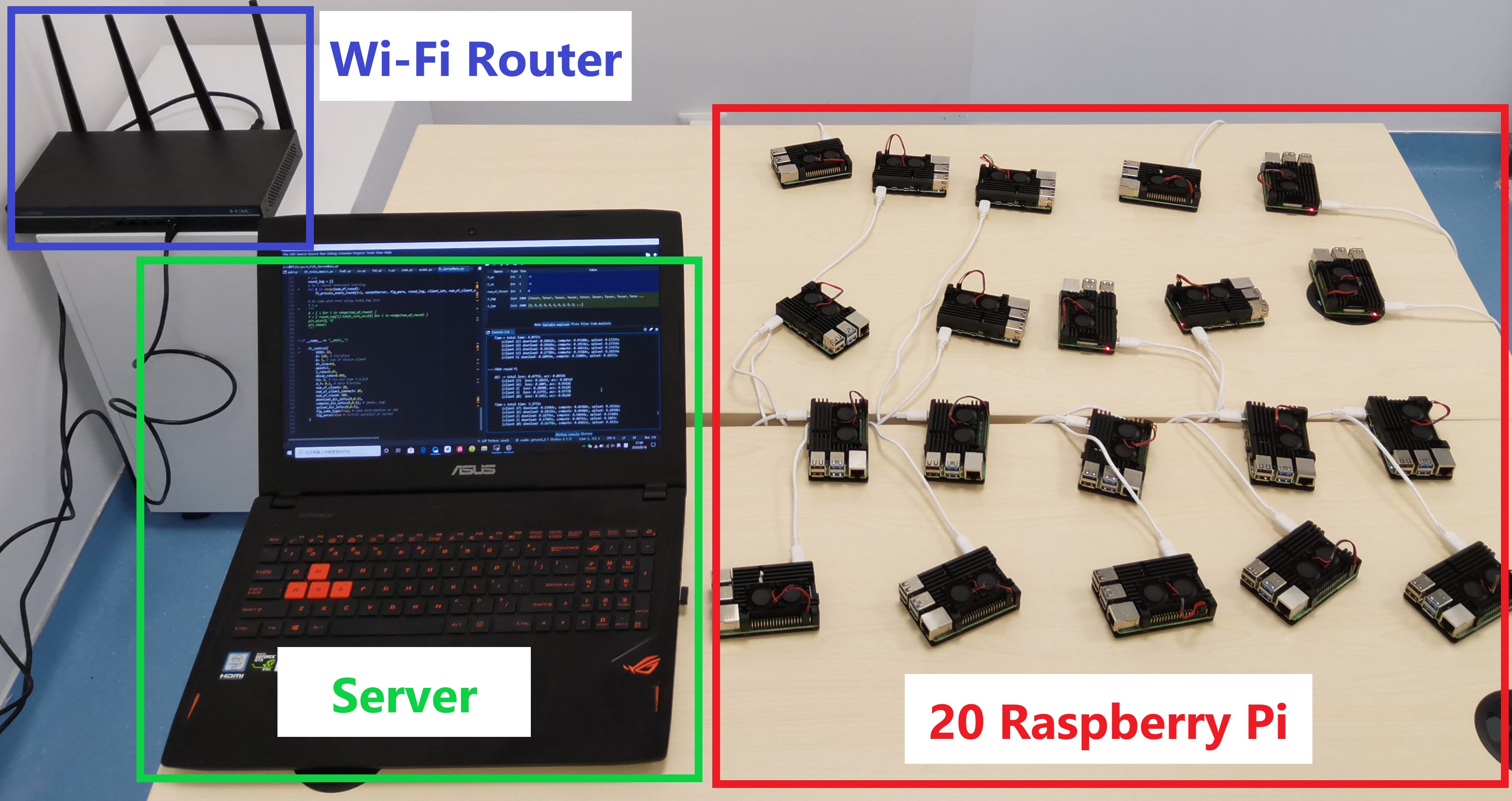
Figure 2: Hardware prototype with the laptop being central server, 20 Raspberry Pi being devices. During the FL experiments, the wireless router is placed 5 meters away from all the devices.

VI Experimental Evaluation

In this section, we evaluate the performance of our proposed cost-effective FL algorithm and verify our derived solution properties. We start by presenting the evaluation setup, and then show the experimental results.

TABLE I: Number of rounds for reaching estimation loss $F_{a}$ and $F_{b}$ for estimation of $\frac{A_{0}}{B_{0}}$ for three Setups

Setup 1	Estimation loss $F_{a}=0.6$ ​$F_{b}=0.5$	Samples of $\left(K,E\right)$	$\left(10,50\right)$	$\left(15,150\right)$	$\left(20,100\right)$	$\left(10,200\right)$	$\left(20,300\right)$	-	-	Estimated $\frac{A_{0}}{B_{0}}$=73,560
		Rounds to achieve $F_{a}$	48	28	32	27	20	-	-
		Rounds to achieve $F_{b}$	82	46	56	43	35	-	-
Setup 2	Estimation loss $F_{a}=0.3$ $F_{b}=0.2$	Samples of $\left(K,E\right)$	$\left(10,10\right)$	$\left(20,20\right)$	$\left(30,30\right)$	$\left(40,40\right)$	$\left(50,50\right)$	$\left(60,60\right)$	$\left(80,80\right)$	Estimated $\frac{A_{0}}{B_{0}}$=3,140
		Rounds to achieve $F_{a}$	67	37	25	22	18	17	16
		Rounds to achieve $F_{b}$	100	60	39	34	28	25	24
Setup 3	Estimation loss $F_{a}=1.5$ $F_{b}=1.3$	Samples of $\left(K,E\right)$	$\left(10,10\right)$	$\left(20,20\right)$	$\left(30,30\right)$	$\left(40,40\right)$	$\left(50,50\right)$	$\left(60,60\right)$	$\left(80,80\right)$	Estimated $\frac{A_{0}}{B_{0}}$=3,750
		Rounds to achieve $F_{a}$	52	39	34	31	30	30	29
		Rounds to achieve $F_{b}$	106	68	57	52	49	48	48

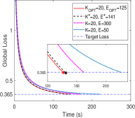
(a) Loss with different $E$

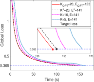
(b) Loss with different $K$

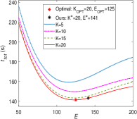
(c) $t_{\textnormal{tot}}$ with different $\left(K,E\right)$

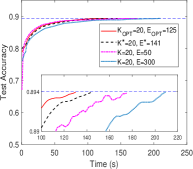
(d) Accuracy with different $E$

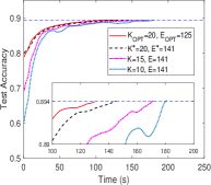
(e) Accuracy with different $K$

Figure 3: Training performance of Setup 1 with logistic regression and MNIST for $\gamma\!=\!0$. (a)-(c): Our solution achieves the target loss $0.365$ using $145.2$s compared to the optimum $141.5$s with optimality error rate $2.61\%$, but faster than those with $E$ being too small or too large and those with $K$ being small. (d)-(e): Our solution achieves $89.4\%$ test accuracy slightly longer than the optimal solution, but faster than the non-optimal values of $\left(K,E\right)$ in (a) and (b).

VI-A Experimental Setup

VI-A1 Platforms

We conducted experiments both on a networked hardware prototype system and in a simulated environment. Our prototype system, as illustrated in Fig. 2, consists of $N=20$ Raspberry Pis (version 4) serving as devices and a laptop computer serving as the central server. All devices are interconnected via an enterprise Wi-Fi router, and we developed a TCP-based socket interface for the peer-to-peer connection. In the simulation system, we simulated $N=100$ virtual devices and a virtual central server.

VI-A2 Datasets and Models

We evaluate our results both on a real dataset and a synthetic dataset. For the real dataset, we adopted the widely used MNIST dataset [42], which contains square $28\times 28=784$ pixel gray-scale images of $70,000$ handwritten digits ($60,000$ for training and $10,000$ for testing). For the synthetic dataset, we follow a similar setup to that in [10], which generates $60$-dimensional random vectors as input data. The synthetic data is denoted by $Synthetic\ (\alpha,\beta)$ with $\alpha$ and $\beta$ representing the statistical heterogeneity (i.e., how non-i.i.d. the data are). We adopt both the convex multinomial logistic regression model [11] and the non-convex deep convolutional neural network (CNN) model with LeNet-5 architecture [42].

VI-A3 Implementation

Based on the above, we consider the following three experimental setups.

Setup 1: We conduct the first experiment on the prototype system using logistic regression and MNIST dataset, where we divide $6,000$ data samples (randomly sampled one-tenth of the total samples) among $N\!=\!20$ Raspberry Pis in a non-i.i.d. fashion with each device containing a balanced number of $300$ samples of only $2$ digits labels.

Setup 2: We conduct the second experiment in the simulated system using CNN and MNIST dataset, where we divide all $60,000$ data samples among $N\!=\!100$ devices in the same non-i.i.d fashion as in Setup 1, but the amount of data in each device follows the inherent unbalanced digit label distribution of MNIST, where the number of samples in each device has a mean of $600$ and standard deviation of $20.1$.

Setup 3: We conduct the third experiment in the simulated system using logistic regression and $Synthetic\ (1,1)$ dataset for statistical heterogeneity, where we generate $24,517$ data samples and distribute them among $N\!=\!100$ devices in an unbalanced power law distribution, where the number of samples in each device has a mean of $245$ and standard deviation of $362$.

VI-A4 Training Parameters

For all experiments, we initialize our model with $\mathbf{w}_{0}=\mathbf{0}$ and SGD batch size $b=64$. In each round, we uniformly sample $K$ devices at random, which run $E$ steps of SGD in parallel. For the prototype system, we use an initial learning rate $\eta_{0}=0.01$ with a fixed decay rate of $0.996$. For the simulation system, we use decay rate $\frac{{\eta}_{0}}{1+r}$, where $\eta_{0}=0.1$ and $r$ is communication round index. We evaluate the aggregated model in each round on the global loss function. Each result is averaged over 50 experiments.

VI-A5 Heterogeneous System Parameters

The prototype system allows us to capture real system heterogeneity in terms of communication and computation time, which we measured the average $t_{p}\!=\!3.1\times 10^{-3}$s with standard deviation $2.3\times 10^{-4}$s and $t_{m}\!=\!0.34$s with standard deviation $1.56\times 10^{-3}$s. We do not capture the energy cost in the prototype system because it is difficult to measure. For the simulation system, we generate the learning time and energy consumption for each client $k$ using a normal distribution with mean $t_{p}\!=\!0.1$s, $t_{m}\!=\!2$s, $e_{p}\!=\!10^{-3}$J, and $e_{m}\!=\!2\times 10^{-2}$J and standard deviation of the mean divided by $3$. According to the definition of $\gamma$, we unify the time and energy costs such that one second is equivalent to $1-\gamma$ dollars ($) and one Joule is equivalent to $\gamma$ dollars ($).

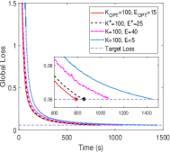
(a) Loss with different $E$

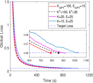
(b) Loss with different $K$

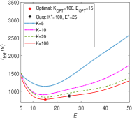
(c) $t_{\textnormal{tot}}$ with different $\left(K,E\right)$

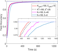
(d) Accuracy with different $E$

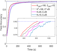
(e) Accuracy with different $K$

Figure 4: Training performance of Setup 2 with CNN and MNIST for $\gamma\!=\!0$. (a)-(c): Our solution achieves the target loss $0.06$ using $856.8$s compared to the optimum $789.0$s with optimality error rate $8.49\%$, but faster than those with $E$ being too small or too large and those with $K$ being small. (d)-(e): Our solution achieves $98.2\%$ test accuracy with almost the same time as the optimal solution, but faster than the non-optimal values of $\left(K,E\right)$ in (a) and (b).

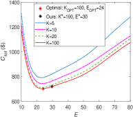
(a) $\gamma=0$

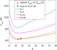
(b) $\gamma=0.45$

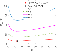
(c) $\gamma=1$

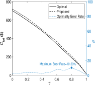
(d) $C_{\textnormal{tot}}$ with $\gamma$

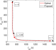
(e) $t_{\textnormal{tot}}$ and $e_{\textnormal{tot}}$ trade-off

Figure 5: Performance of $C_{\textnormal{tot}}$ for reaching the target loss 1.05 for Setup 3 with logistic regression and Synthetic (1,1). (a)-(d) When $\gamma$ increases from $0$ to $1$, our solutions reaches the target loss using the similar cost as the corresponding optimal ones, with average optimality error rate $4.85\%$ and maximum rate $10.23\%$. (e) For different $\gamma$, our proposed solutions are able to balance the metric preferences between $t_{\textnormal{tot}}$ and $e_{\textnormal{tot}}$ while approaching the optimal trade-off.

VI-B Performance Results

We first validate the optimality of our proposed solution with estimated value of $\frac{A_{0}}{B_{0}}$. Then, we show the impact of the trade-off factor $\gamma$, followed by the verification of our derived theoretical properties.

VI-B1 Estimation of $\frac{A_{0}}{B_{0}}$

We summarize the estimation process and results of $\frac{A_{0}}{B_{0}}$ for all three experiment setups in Table I. Specifically, using Algorithm 2, we empirically set two relatively high target losses $F_{a}$ and $F_{b}$ with a few sampling pairs of $\left(K,E\right)$. Then, we record the corresponding number of rounds for reaching $F_{a}$ and $F_{b}$, based on which we calculate the averaged estimation value of $\frac{A_{0}}{B_{0}}$ using (25). The proposed solution $K^{*}$ and $E^{*}$ is then obtained from Algorithm 2. For comparison, we denote $K_{\textnormal{OPT}}$ and $E_{\textnormal{OPT}}$ as the empirical optimal solution achieved by exhaustive search on $\left(K,E\right)$.

VI-B2 Convergence and Optimality

Figs. 3 and 4 show the learning time cost for reaching the target loss under different $\left(K,E\right)$ for Setups 1 and 2, respectively. In both setups, our proposed solutions achieve near-optimal performance compared to the empirical optimal solution, with optimality error of $2.61\%$ and $8.49\%$, respectively. We highlight that our approach works well with the non-convex CNN model in Setup 2. Although the error rate in Setup 2 is higher than that in Setup 1, note that non-optimal values of $(K,E)$ without optimization may increase the learning time by several folds.

Fig. 5 depicts the performance of $C_{\textnormal{tot}}$ for achieving the target loss with $\gamma$ under different $\left(K,E\right)$ in Setup 3, where our proposed solutions achieve near-optimal performance for all values of $\gamma$. Particularly, Fig. 5(d) shows that, throughout the range of $\gamma$, our approach has the maximum optimality error of $10.23\%$ and an average error of $4.85\%$.

VI-B3 Impact of Weight $\gamma$

Figs. 5(a) – 5(c) show that when the weight $\gamma$ increases from $0$ to $1$ (corresponding to the design preference varying from reducing learning time to saving energy consumption), both the optimal and our proposed solutions of $K$ decrease from $N\!=\!100$ to $1$. At the same time, both the optimal and our proposed solutions of $E$, although with a small difference, decrease slightly as $\gamma$ increases. We give the explanations of these observations in Section VI-B4 below. By iterating through the entire range of $\gamma$, Fig. 5(e) depicts the trade-off curve between the learning time cost and energy consumption cost, where our algorithm is capable of balancing the two metrics as well as approaching the optimal.

VI-B4 Property Validation

We highlight that our derived theoretical properties of $K$ and $E$ in Section V can be validated empirically, which we summarize as follows.

• Figs. 3(c), 4(c), and 5(a) demonstrate that for any fixed value $E$, the learning time cost ($\gamma\!=\!0$) strictly decreases in $K$, which confirms the claim in Theorem 2 that sampling more clients can speed up learning. Moreover, we observe in these figures that sampling fewer clients (15 out of 20 for Setup 1 and 20 out of 100 for Setups 2 and 3) does not affect the learning time much, which confirms our Remark. Nevertheless, Fig. 5(c) shows that for any fixed value $E$, the energy consumption cost ($\gamma\!=\!1$) strictly increases in $K$, which confirms Theorem 3 that sampling fewer clients reduces energy consumption.

• Figs. 3(c), 4(c), 5(a)–5(c) demonstrate that, for any fixed value of $K$, the corresponding cost first decreases and then increases as $E$ increases, which confirms Corollaries 1 and 3 as well as the biconvex property in Theorem 1. Since $\frac{e_{m}}{t_{m}}=\frac{e_{p}}{t_{p}}=10^{-2}$ in our simulation system, we observe from Figs. 3(c), 4(c), and 5(a) that both $K^{\ast}$ and $E^{\ast}$ decrease as $\gamma$ increases, which confirms Theorem 4.

VII Conclusion

In this work, we have studied the cost-effective design for FL. We analyzed how to optimally choose the number of participating clients ($K$) and the number of local iterations ($E$), which are two essential control variables in FL, to minimize the total cost while ensuring convergence. We proposed a sampling-based control algorithm which efficiently solves the optimization problem with marginal overhead. We also derived insightful solution properties which helps identify the design principles for different optimization goals, e.g., reducing learning time or saving energy. Extensive experimentation results validated our theoretical analysis and demonstrated the effectiveness and efficiency of our control algorithm. Our optimization design is orthogonal to most works on resource allocation for FL systems, and can be used together with those techniques to further reduce the cost.

References

- [1] P. Kairouz, H. B. McMahan, B. Avent, A. Bellet, M. Bennis, A. N. Bhagoji, K. Bonawitz, Z. Charles, G. Cormode, R. Cummings et al., “Advances and open problems in federated learning,” arXiv preprint arXiv:1912.04977, 2019.
- [2] B. McMahan, E. Moore, D. Ramage, S. Hampson, and B. A. y Arcas, “Communication-efficient learning of deep networks from decentralized data,” in Artificial Intelligence and Statistics, 2017, pp. 1273–1282.
- [3] J. Konečnỳ, H. B. McMahan, D. Ramage, and P. Richtárik, “Federated optimization: Distributed machine learning for on-device intelligence,” arXiv preprint arXiv:1610.02527, 2016.
- [4] Q. Yang, Y. Liu, T. Chen, and Y. Tong, “Federated machine learning: Concept and applications,” ACM Transactions on Intelligent Systems and Technology (TIST), vol. 10, no. 2, pp. 1–19, 2019.
- [5] T. Li, A. K. Sahu, A. Talwalkar, and V. Smith, “Federated learning: Challenges, methods, and future directions,” IEEE Signal Processing Magazine, vol. 37, no. 3, pp. 50–60, 2020.
- [6] J. Park, S. Samarakoon, M. Bennis, and M. Debbah, “Wireless network intelligence at the edge,” Proceedings of the IEEE, vol. 107, no. 11, pp. 2204–2239, 2019.
- [7] F. Sattler, S. Wiedemann, K.-R. Müller, and W. Samek, “Robust and communication-efficient federated learning from non-iid data,” IEEE Transactions on Neural Networks and Learning Systems, 2019.
- [8] K. Bonawitz, H. Eichner, W. Grieskamp, D. Huba, A. Ingerman, V. Ivanov, C. Kiddon, J. Konečnỳ, S. Mazzocchi, H. B. McMahan et al., “Towards federated learning at scale: System design,” in Systems and Machine Learning (SysML) Conference, 2019.
- [9] V. Smith, C.-K. Chiang, M. Sanjabi, and A. S. Talwalkar, “Federated multi-task learning,” in Advances in Neural Information Processing Systems (NeurIPS), 2017, pp. 4424–4434.
- [10] T. Li, A. K. Sahu, M. Zaheer, M. Sanjabi, A. Talwalkar, and V. Smith, “Federated optimization in heterogeneous networks,” in Machine Learning and Systems (MLSys) Conference, 2020.
- [11] X. Li, K. Huang, W. Yang, S. Wang, and Z. Zhang, “On the convergence of fedavg on non-iid data,” in International Conference on Learning Representations (ICLR), 2019.
- [12] N. H. Tran, W. Bao, A. Zomaya, N. M. NH, and C. S. Hong, “Federated learning over wireless networks: Optimization model design and analysis,” in IEEE Conference on Computer Communications (INFOCOM), 2019, pp. 1387–1395.
- [13] S. Wang, T. Tuor, T. Salonidis, K. K. Leung, C. Makaya, T. He, and K. Chan, “Adaptive federated learning in resource constrained edge computing systems,” IEEE Journal on Selected Areas in Communications, vol. 37, no. 6, pp. 1205–1221, 2019.
- [14] J. Wang and G. Joshi, “Adaptive communication strategies to achieve the best error-runtime trade-off in local-update SGD,” in Systems and Machine Learning (SysML) Conference, 2019.
- [15] K. Bonawitz, V. Ivanov, B. Kreuter, A. Marcedone, H. B. McMahan, S. Patel, D. Ramage, A. Segal, and K. Seth, “Practical secure aggregation for federated learning on user-held data,” in NeurIPS Workshop on Private Multi-Party Machine Learning, 2016.
- [16] B. Avent, A. Korolova, D. Zeber, T. Hovden, and B. Livshits, “BLENDER: Enabling local search with a hybrid differential privacy model,” in USENIX Security Symposium (USENIX Security), 2017, pp. 747–764.
- [17] J. Konečnỳ, H. B. McMahan, F. X. Yu, P. Richtárik, A. T. Suresh, and D. Bacon, “Federated learning: Strategies for improving communication efficiency,” in NeurIPS Workshop on Private Multi-Party Machine Learning, 2016.
- [18] M. Abadi, A. Agarwal, P. Barham, E. Brevdo, Z. Chen, C. Citro, G. S. Corrado, A. Davis, J. Dean, M. Devin et al., “Tensorflow: Large-scale machine learning on heterogeneous distributed systems,” arXiv preprint arXiv:1603.04467, 2016.
- [19] H. Yu, S. Yang, and S. Zhu, “Parallel restarted SGD for non-convex optimization with faster convergence and less communication,” in AAAI Conference on Artificial Intelligence, 2019.
- [20] S. U. Stich, “Local SGD converges fast and communicates little,” in International Conference on Learning Representations (ICLR), 2018.
- [21] J. Wang and G. Joshi, “Cooperative SGD: A unified framework for the design and analysis of communication-efficient SGD algorithms,” in ICML Workshop on Coding Theory for Machine Learning, 2019.
- [22] A. Khaled, K. Mishchenko, and P. Richtárik, “First analysis of local GD on heterogeneous data,” arXiv preprint arXiv:1909.04715, 2019.
- [23] F. Zhou and G. Cong, “On the convergence properties of a k-step averaging stochastic gradient descent algorithm for nonconvex optimization,” in International Joint Conference on Artificial Intelligence (IJCAI), 2018, pp. 3219–3227.
- [24] W. Liu, L. Chen, Y. Chen, and W. Zhang, “Accelerating federated learning via momentum gradient descent,” IEEE Transactions on Parallel and Distributed Systems, vol. 31, no. 8, pp. 1754–1766, 2020.
- [25] S. Samarakoon, M. Bennis, W. Saad, and M. Debbah, “Federated learning for ultra-reliable low-latency V2V communications,” in IEEE Global Communications Conference (GLOBECOM), 2018, pp. 1–7.
- [26] G. Zhu, Y. Wang, and K. Huang, “Broadband analog aggregation for low-latency federated edge learning,” IEEE Transactions on Wireless Communications, vol. 19, no. 1, pp. 491–506, 2019.
- [27] T. Nishio and R. Yonetani, “Client selection for federated learning with heterogeneous resources in mobile edge,” in IEEE International Conference on Communications (ICC), 2019, pp. 1–7.
- [28] H. Wang, Z. Kaplan, D. Niu, and B. Li, “Optimizing federated learning on non-iid data with reinforcement learning,” in IEEE Conference on Computer Communications (INFOCOM), 2020, pp. 1698–1707.
- [29] W. Shi, S. Zhou, and Z. Niu, “Device scheduling with fast convergence for wireless federated learning,” in IEEE International Conference on Communications (ICC), 2020, pp. 1–6.
- [30] M. Chen, H. V. Poor, W. Saad, and S. Cui, “Convergence time optimization for federated learning over wireless networks,” arXiv preprint arXiv:2001.07845, 2020.
- [31] P. Han, S. Wang, and K. K. Leung, “Adaptive gradient sparsification for efficient federated learning: An online learning approach,” in IEEE International Conference on Distributed Computing Systems (ICDCS), 2020.
- [32] Y. Jiang, S. Wang, V. Valls, B. J. Ko, W.-H. Lee, K. K. Leung, and L. Tassiulas, “Model pruning enables efficient federated learning on edge devices,” in Workshop on Scalability, Privacy, and Security in Federated Learning (SpicyFL) in Conjunction with NeurIPS, 2020.
- [33] X. Mo and J. Xu, “Energy-efficient federated edge learning with joint communication and computation design,” arXiv preprint arXiv:2003.00199, 2020.
- [34] Q. Zeng, Y. Du, K. Huang, and K. K. Leung, “Energy-efficient resource management for federated edge learning with CPU-GPU heterogeneous computing,” arXiv preprint arXiv:2007.07122, 2020.
- [35] Z. Yang, M. Chen, W. Saad, C. S. Hong, and M. Shikh-Bahaei, “Energy efficient federated learning over wireless communication networks,” arXiv preprint arXiv:1911.02417, 2019.
- [36] Y. Tu, Y. Ruan, S. Wang, S. Wagle, C. G. Brinton, and C. Joe-Wang, “Network-aware optimization of distributed learning for fog computing,” arXiv preprint arXiv:2004.08488, 2020.
- [37] W. Luping, W. Wei, and L. Bo, “CMFL: Mitigating communication overhead for federated learning,” in IEEE International Conference on Distributed Computing Systems (ICDCS), 2019, pp. 954–964.
- [38] K. Hsieh, A. Harlap, N. Vijaykumar, D. Konomis, G. R. Ganger, P. B. Gibbons, and O. Mutlu, “Gaia: Geo-distributed machine learning approaching LAN speeds,” in USENIX Symposium on Networked Systems Design and Implementation (NSDI), 2017, pp. 629–647.
- [39] Y. Jin, L. Jiao, Z. Qian, S. Zhang, S. Lu, and X. Wang, “Resource-efficient and convergence-preserving online participant selection in federated learning,” in IEEE International Conference on Distributed Computing Systems (ICDCS), 2020.
- [40] J. Gorski, F. Pfeuffer, and K. Klamroth, “Biconvex sets and optimization with biconvex functions: a survey and extensions,” Mathematical methods of operations research, vol. 66, no. 3, pp. 373–407, 2007.
- [41] K.-H. Schlote, “Bl van der waerden, moderne algebra, (1930–1931),” in Landmark Writings in Western Mathematics 1640-1940. Elsevier, 2005, pp. 901–916.
- [42] Y. LeCun, L. Bottou, Y. Bengio, and P. Haffner, “Gradient-based learning applied to document recognition,” Proceedings of the IEEE, vol. 86, no. 11, pp. 2278–2324, 1998.