Can the zero-point energy of the quantized harmonic oscillator be lower?
Possible implications for the physics of “dark energy” and “dark matter”

Abstract

Replacing the canonical pair $q$ and $p$ of the classical harmonic oscillator (HO) by the locally and symplectically equivalent pair angle $\varphi$ and action variable $I$ implies a qualitative change of the global topological structure of the associated phase spaces: the pair $(q,p)$ is an element of a topologically trivial plane $\mathbb{R}^{2}$ whereas the pair $(\varphi,I>0)\in\mathbb{S}^{1}\times\mathbb{R}_{+}$ is an element of a topologically non-trivial, infinitely connected, $punctured$ plane $\mathbb{R}^{2}-\{0\}$, which has the orthochronous “Lorentz” group $SO^{\uparrow}(1,2)$ (or its two-fold covering, the symplectic group $Sp(2,\mathbb{R})$) as its “canonical” group. Due to its infinitely many covering groups the resulting (“symplectic”) spectrum of the associated quantum Hamiltonian $H=\omega\,\hat{I}$ is given by $\{\hbar\omega(n+b),n=0,1,\ldots;\,b\in(0.1],\text{e.g.\ $b=1/s,\,s\in\mathbb{N}$ and large}\}$, in contrast to the $(q,p)$ version, where the Hamiltonian has the “orthodox” spectrum $\{\hbar\omega(n+1/2)\}$. The deeper reason for the difference is that for the description of the periodic orbit $\{p=p(q)\}$ one covering of $\mathbb{S}^{1}$ suffices, whereas one generally needs many coverings for the time evolution $\varphi(t)$. And this, in turn, can lead to a lowering of the zero-point energies.

Several theoretical and possible experimental implications of the “symplectic” spectra of the HO are discussed: The potentially most important ones concern the vibrations of diatomic molecules in the infrared, e.g. those of molecular hydrogen H₂. Those symplectic spectra of the HO may provide a simultaneous key to two outstanding astrophysical puzzles, namely the nature of dark (vacuum) energy and that of dark matter: To the former because the zero-point energy $b\,\hbar\omega$ of free electromagnetic wave oscillator modes can be extremely small $>0$ $(b\approx\exp{(-35)}$ for the measured dark energy density). And a key to the dark matter problem because the quantum zero-point energies of the electronic Born-Oppenheimer potentials in which the two nuclei of H₂ or the nuclei of other primordial diatomic molecules vibrate can be lower, too, and, therefore, may lead to spectrally detuned “dark” H₂ molecules during the “Dark Ages” of the universe and forming WIMPs in the hypothesized sense! All results appear to be in surprisingly good agreement with the $\Lambda$CDM model of the universe.

Besides laboratory experiments the search for 21-cm radio signals from the Dark Ages of the universe and other astrophysical observations can help to explore those hypothetical implications.

I Introduction

It very probably appears presumptuous and provocative to question the well-known quantum properties of the primeval prototype of quantum mechanical systems: the harmonic oscillator (HO in the following)!

The motive for daring a new look at the physical system HO arise from its well-known locally - but not globally - equivalent canonical descriptions: either in terms of the Cartesian coordinates $(q,p)\in\mathbb{R}^{2}$ or in terms of the angle and action variables $(\varphi,I)\in\{\mathbb{R}\bmod{2\pi}\times\mathbb{R}^{+}\}\cong\mathbb{S}^{1}\times\mathbb{R}^{+}\cong\mathbb{R}^{2}-\{0\}$, where $x\in\mathbb{R}^{+}$ iff $x\in\mathbb{R}$ and $x>0$, the relationship of which can be defined by kas (a)

$$q(\varphi,I)=\sqrt{\frac{2\,I}{m\,\omega}}\,\cos\varphi\,,~{}~{}p(\varphi,I)=-\sqrt{2\,m\,\omega\,I}\,\sin\varphi\,.$$ (1)

This mapping is locally symplectic:

$$dq\wedge dp=d\varphi\wedge dI\,,~{}~{}\text{or}~{}~{}\frac{\partial(q,p)}{\partial(\varphi,I)}=1\,.$$ (2)

The canonically equivalent Hamiltonians are given by

$$H(q,p)=\frac{1}{2m}\,p^{2}+\frac{1}{2}\,m\,\omega^{2}\,q^{2}=H(\varphi,I)=\omega\,I\,,$$ (3)

with their respective canonical Eqs. of motion

$$\dot{q}= \frac{\partial H}{\partial p}=p/m,~{}~{}~{}\dot{p}=-\frac{\partial H}{\partial q}=-m\omega^{2}q\,;$$ (4)

$$\dot{\varphi}= \frac{\partial H}{\partial I}=\omega,~{}~{}~{}\dot{I}=-\frac{\partial H}{\partial\varphi}=0,$$ (5)

the latter with the obvious solutions

$$\varphi(t)=\omega\,t+\varphi_{0}\,,~{}~{}I=\text{ const.}=I_{0}=E/\omega>0\,.$$ (6)

The solutions of the Eqs. (4) and (5) describe - as functions of time $t$ - orbits in the repective phase spaces

$$\mathcal{S}_{q,p} = \{(q,p)\in\mathbb{R}^{2}\,\}\cong\mathbb{R}^{2}\,$$ (7)

$$\text{ and }~{}~{}\mathcal{S}_{\varphi,I} = \{(\varphi,I),\varphi\in\mathbb{R}\bmod{2\pi}\,,\,I>0\,\}$$

$$\cong S^{1}\times\mathbb{R}^{+}\cong\mathbb{R}^{2}-\{0\}\,.$$

The crucial point - for all what follows in the present paper - is this: the two phase spaces (7) and (I) are globally (topologically) qualitatively different! Whereas the $(q,p)$-space is a simply connected and topologically trivial plane $\mathbb{R}^{2}$, the $(\varphi,I)$-space is topologically a “punctured” plane, i.e. a $\mathbb{R}^{2}$ with the origin $\{(0,0)\}$ deleted!

This is so for several reasons: the variables $\varphi$ and $I$ can be considered as polar coordinates of a plane, with - obviously - $\varphi$ the angle and $I>0$ the radial variable. The value $I=0$ has to be excluded because otherwise the angle $\varphi$ becomes undefined at that point. In addition the value $I=0$ describes a branch point for the transformation functions (1). More arguments can be found in Ref. Kastrup (2007).

The topology of the phase space (I) may equivalently be characterized as that of a simple cone with the tip deleted or as that of a semi-cylinder without the points of the finite circular surface at $I=0$.

If $\varphi(t)$ and $I(t)$ describe the moving points of a periodic orbit on $\mathcal{S}_{\varphi,I}$ then those points may loop around the origin arbitrarily many times (the first homotopy group $\pi_{1}$ of $\mathcal{S}_{\varphi,I}$ consists of the integers $\in\mathbb{Z}$), because the orbit coordinate $\varphi(t)$ can circle the origin of $\mathbb{S}^{1}$ arbitrarily many times in the course of time $t$! Thus, the configuration space of $\varphi$ corresponds to one of the infinitely many covering spaces of the circle $\mathbb{S}^{1}$, the universal covering being the real line $\mathbb{R}$. A physical example for a high number of coverings is provided by the oscillations of electromagnetic vibrations.

That missing point in the phase space $\mathbb{R}^{2}_{0}\equiv\mathcal{S}_{q,p}-\{0,0\}$, or in $\mathcal{S}_{\varphi,I}$, has dramatic consequences for the associated quantum theory which will be discussed in more detail below.

The crucial result is the following:

The quantum operator version $\hat{I}=K_{0}$ of the classical action variable $I$ of the HO has the possible spectrum

$$K_{0}|b,n\rangle=\hbar(n+b)|b,n\rangle,\,\,n=0,1,2,\ldots;\ 1>b>0.$$ (9)

Here $K_{0}$ is the self-adjoint Lie algebra generator of the compact subgroup O(2) in an irreducible unitary representation of the 3-dimensionsl “orthochronous Lorentz” group $SO^{\uparrow}(1,2)\cong Sp(2,\mathbb{R})/Z_{2}$ or of one of its infinitely many covering groups, where the double covering $Sp(2,\mathbb{R})$ is the symplectic group of the plane. (see below). This means that the HO Hamilton operator

$$H_{\varphi,I}=\omega\,K_{0},$$ (10)

associated with the phase space $\mathcal{S}_{\varphi,I}$, can have a ground state ($n=0$) with eigenvalue (zero-point energy) $\hbar\omega\,b,\,1>b>0$, especially with $1/2>b>0$ !

As indicated above, the mathematical origin of this possibility is a group theoretical one: The “canonical” transformation group of the punctured plane $\mathbb{R}^{2}_{0}$ is the symplectic group $Sp(2,\mathbb{R})$ which acts transitively on $\mathbb{R}^{2}_{0}$ (for any two points on $\mathbb{R}^{2}_{0}$ there is an element of $Sp(2,\mathbb{R})$ which connects the two but leaves the origin invariant)!

The group $Sp(2,\mathbb{R})$ is a twofold covering of the “orthochronous Lorentz” group $SO^{\uparrow}(1,2)$ in “one time and two space dimensions” which acts correspondingly on the phase space $\mathcal{S}_{\varphi,I}$, i.e. acting transitively and leaving the origin invariant! The number $b,\,1>b>0$ in Eq. (9) characterizes an irreducible unitary representation of a given covering group of $SO^{\uparrow}(1,2)$ kas (b).

The main mathematical aspects of the present paper have been presented previously in Refs. Bojowald et al. (2000); Bojowald and Strobl (2000); Kastrup (2003, 2007); Bojowald and Strobl (2003). A brief - introductory but probably helpful - summary of them is given in Ref. Kastrup (2011). Essential mathematical references are Bargmann (1947); Pukánszky (1964); Vilenkin (1968); P. J. Sally (1967, 1970); Boyer and Wolf (1975).

The present paper tries to draw attention to possible experimental and observational implications of the $(\varphi,I)$-framework for the HO. Hopefully, appropriate laboratory experiments and astrophysical obervations will be able to find out whether nature has “made use of the available mathematical possibilities”(Dirac) or not!

There are - at least - two immediate crucial questions:

i) Why should the classical canonical pair $(\varphi,I)$ be a “better” - or at least equivalent - basis for the quantum description of a system like the HO, compared to the conventional pair $(q,p)$?

ii) If the predictions of the quantized $(\varphi,I)$ framework are richer than the $(q,p)$ framework - but not contradictory -, why haven’t they been observed yet?

Ad i): A crucial obstacle for using the “observable” angle $\varphi$ itself for the quantum description of a physical system has been that there exist no corresponding self-adjoint operator $\hat{\varphi}$ Kastrup (2006, 2016)! This shortcoming can, however, be remedied by the following observation Kastrup (2006, 2016):

Geometrically an angle $\varphi$ can be defined by two oriented rays (vectors) both originating from the same given point. The two rays then span a plane. In order to describe the angle uniquely analytically one chooses a third ray which “emanates” from the same point and which is orthogonal to one of the two original rays. Projecting the second original ray onto the two orthogonal ones by means of a circle, with radius $a$, around the origin yields a pair $a(\cos\varphi,\sin\varphi),\,a>0,$ which determines $\varphi$ uniquely, after chosing a clockwise- or counter-clockwise orientation. It is convenient, but not necessary, to put $a=1$.

Quantizing the system then means: quantizing the components $a\cos\varphi$ and $a\sin\varphi$ which combined represent one “observable”, the angle $\varphi\,$! The details depend on the choice of $a$ and possibly other elements of the associated Poisson algebra.

We now come to a crucial physical point:

For periodic motions - like that of a HO - the angle $\varphi(t)$ of Eq. (5) does not stop at $\varphi(T)\equiv\omega\,T=2\pi$ but “runs” around the origin, say at least $s$ times, i.e. $\varphi(t)\geq\varphi(t_{s})=s\,2\pi,\,s\in\mathbb{Z},$, and in this way generates an (s+1)-fold covering of the unit circle $\mathbb{S}^{1}$. In this way the configuration space $\mathbb{S}^{1}_{[s+1]}$ of the angle becomes (s+1)-fold connected, and, as $s$ can be an arbitrary integer, infinitely connected.

So, for dynamical (time-dependent) periodic systems the “observable” angle consists of 2 parts: the number $s$ of completed coverings $\mathbb{S}^{1}_{[s]}$ of the unit circle and a “rest” $\chi\in[0,2\pi)$:

$$\varphi=(2\pi\,s+\chi)\in\mathbb{S}^{1}_{[s+1]},~{}s\in\mathbb{Z},~{}\chi\in[0,2\pi).$$ (11)

The crucial point for periodic motions is that $s=0$ is sufficient to describe the orbit $p(q)$ of Eq. (1), but in order to describe the time evolution $\varphi(t)$ one needs to know the pair $(\chi;s)$ of Eq. (11). This is a consequence of the non-trivial topology of the phase space (I). In many cases the angle $\varphi(t)$ appears in the form $\varphi(t)=\omega t\equiv\tilde{t}$, i.e. it is essentially a time variable. Thus, the pair $(q,p)\in\mathcal{S}_{q,p}$ of a periodic orbit is independent of the number $s$ of coverings. But this number of coverings is essential in connection with the phase space $\mathcal{S}_{\varphi,I}$. This important difference leads to corresponding different quantum mechanical properties of the two phase spaces, e.g. for $\mathcal{S}_{\varphi,I}$ to the set of spectra (9), containing the “orthodox” case $b=1/2$ as a special one! We shall see that an $s$-fold covering ($s>0$ ) is associated with $b=1/s$.

The introduction of the canonical pair angle and action variables is conventionally motivated by the aim to make the action variable $I$ a constant of motion, i.e. to have an “integrable” system Landau and Lifshitz (1969); Thirring (1997, pb: 2003); Arnold et al. (2006). But this is not necessary: one can try to describe systems in the phase space (I) in terms of the local coordinate pair $(\varphi,I)$ or the global ones $h_{0}=I,.\,h_{1}=I\cos\varphi,\,h_{2}-I\sin\varphi$ which will be illustrated by an example in the next chapter.

Phases play an important role in many physical systems with periodic properties like vibrations, waves etc., e.g. in optics, atomic and molecular spectroscopy, condensed matter physics etc.  Thus, it is important to understand the corresponding quantum theories in terms of the canonical pair angle and action variable properly and consistently and look for experimental consequences.

Ad ii): One reason might be that nobody up to now has been looking for the newly predicted physical phenomena! Another reason could be that the associated signals are very weak and obscured by the “orthodox” spectrum $\hbar\omega\,(n+1/2)$! Possible related future laboratory experiments are indicated in Ch. IV and associated interpretations of present and future astrophysical observations in Ch. V.

The paper is organized as follows:

Ch. II discusses a few properties of the phase space (I): its global coordinates $h_{j},j=0,1,2$, provided in terms of the group $SO^{\uparrow}(1,2)$. Further the trivial orbits (circles) of the HO on the phase space (I) and those of a dynamical model, a simple generalization on $\mathcal{S}_{\varphi,I}$ of the HO. These “classical” considerations are intended to provide an intuitive background for the discussions of the associated quantum mechanics in Ch. III.

In Ch. III several aspects of quantum mechanical systems are discussed the basic “observables” of which are given by the Lie algebra elements $K_{0},K_{1}$ and $K_{2}$ of the canonical group $Sp(2,\mathbb{R})$ of the punctured plane. Though this Lie algebra is also that of the isomorphic groups $SU(1,1)$ or $SL(2,\mathbb{R})$, of the group $SO^{\uparrow}(1,2)$ and all covering groups as well, the “symplectic” variant appears to be preferable because of possible generalizations to higher dimensional phase spaces Kastrup (2007, 2003).

One of the main topics in this chapter consists of the discussion of the spectrum (9) and related explicit Hilbert spaces for the representation of the self-adjoint operators $K_{0},K_{1},K_{2}$. Extended use is made of mathematical results contained in Refs. Kastrup (2003, 2007). Hardy spaces (i.e. Hilbert spaces which have non-vanishing Fourier components for $n=0,1,2,\ldots$ only) on the circle play a prominent role for constructing those explicit Hilbert spaces.

Ch. IV contains a number of suggestions to find concrete physical systems to which the theoretical framework may apply.

Possibly the most important application concerns the vibrations of diatomic molecules which are harmonic in the neighbourhood of the minima of their Born-Oppenheimer (BO) potentials and where “symplectic” spectra (9) may lead to a lower ($b<1/2$) ground state energy compared to the “orthodox” value $b=1/2$ !

Laboratory tests are, of course, of crucial importance, especially for molecular hydrogen H₂. As this molecule has no permanent electric dipole moment, its “orthodox” infrared emission and absorption signals are already very weak. Therefore very probably even more so the “non-orthodox” ones. Other diatomic molecules of the lightest elements with an electric dipole element (like, e.g. LiH) may be more appropriate for laboratory infrared experiments.

For H₂ itself Raman scattering or atomic and molecular collisions may induce transient electric dipole moments leading to characteristic emissions or absorptions associated with vibrations (and rotations) her (a).

Extremely important are possible astrophysical applications, discussed in Ch. V, especially concerning the problems of dark energy and dark matter; here the spectrum (9) may provide the key to the simultaneous understanding of both problems:

As the index $b$ may be arbitrarily small $>0$, the associated estimate of the cosmological constant $\Lambda$ - or the vacuum “dark” energy density - can be compatible with the experimentally observed value, leading to $b\approx\exp(-35)$ .

In addition, the possible lowering of the vibrational zero-point energies of electronic Born - Oppenheimer potentials for diatomic molecules suggests to look at molecular hydrogen b-H₂ and other primordial diatomic molecules as candidates for dark matter.

Altogether one finds that the consequences of a symplectic spectrum ($0<b<1/2$) of the HO are surprisingly well compatible with the cosmological $\Lambda$CDM model, with - mainly - $b$-H₂ molecules as WIMPs !

There is, however, one important caveat: the dynamics of the transitions (rates) to and from the new additional energy levels has still to be worked out !

Experimentally, 21-cm radio telescopes directed towards the Dark Ages of the universe are of special importance (see, e.g. Ref. et al. (a)). Recent observations et al. (2018a) indicate – unexpected for the present interpretations of dark matter – non-gravitational (electromagnetic?) interactions between atomic hydrogen and dark matter Barkana (2018); Fialkov et al. (2018) ! This appears to be compatible with $b$-H₂ molecules as dark matter Similarly the recently observed discrepancy between computer simulated dark matter models and gravitational lensing et al. (2020a) is of interest in this context.

If the observed cosmic dark matter indeed consists of - infrared detuned - primordial diatomic molecules then there is no need for the introduction of any kind of “new” matter, a point which has also been emphasized in the recent discussions of dark matter as being formed by primordial black holes (for a recent review see, e.g. Ref. Hasinger (2020)).

II Motions on the classical
phase spaces $\mathcal{S}_{\varphi,I}$ and $\mathcal{S}_{q,p}$

The present chapter discusses a simple classical model on the phase space $\mathcal{S}_{\varphi,I}$ as a preparation for the discussion of the corresponding quantum mechanical one later.

II.1 Coordinates and orbits on $\mathcal{S}_{\varphi,I}$

II.1.1 Global coordinates

It was already indicated above that the angle $\varphi$ itself is not a “good” global coordinate on $\mathcal{S}_{\varphi,I}$. The situation is even worse for the corresponding quantum theory Kastrup (2006). As described above, a way out is to characterize the geometrical quantity “angle” by the pair $(\cos\varphi,\sin\varphi)$. However the triple $I,C(\varphi)=\cos\varphi,S(\varphi)=\sin\varphi$ is still not appropriate for our present purpose:

Consider the Poisson brackets

$$\{f_{1},f_{2}\}_{\varphi,I}\equiv\partial_{\varphi}f_{1}\,\partial_{I}f_{2}-\partial_{I}f_{1}\,\partial_{\varphi}f_{2}$$ (12)

for locally smooth functions on $\mathcal{S}_{\varphi,I}$. The 3 functions $I,C(\varphi)$ and $S(\varphi)$ obey the Poisson Lie algebra

$$\{I,C\}_{\varphi,I}=S\,,~{}\{I,S\}_{\varphi,I}=-C\,,~{}\{C,S\}_{\varphi,I}=0\,,$$ (13)

which constitutes the Lie algebra of the Euclidean group $E(2)$ of the plane: rotations (generated by $I$) and 2 independent translations (generated by $C$ and $S$). They are the proper coordinates for a phase space with the topology of an infinite cylinder $\mathbb{S}^{1}\times\mathbb{R}$, like that of the canonical system angle and orbital angular momentum Kastrup (2006, 2016).

It can be justified systematically ka1 (a) that the appropriate global coordinates on $\mathcal{S}_{\varphi,I}$ are the functions

$$h_{0}(\varphi,I) =I>0\,,$$ (14)

$$h_{1}(\varphi,I)=I\cos\varphi\,, \;\;\;h_{2}(\varphi,I)=-I\sin\varphi\,,$$

which obey

$$\vec{h}^{2}\equiv h_{1}^{2}+h_{2}^{2}=h_{0}^{2},\,h_{0}>0.$$ (15)

and, therefore, describe a simple (“light”) cone, with the tip deleted. The functions $h_{j}(\varphi,I)$ obey the Poisson Lie algebra

$$\{h_{0},h_{1}\}_{\varphi,I}=-h_{2}\,, ~{}\{h_{0},h_{2}\}_{\varphi,I}=h_{1}\,,$$ (16)

$$\{h_{1},h_{2}\}_{\varphi,I} =h_{0}\,,$$

which constitutes - as mentioned above - the Lie algebra of the 3-dimensional group $SO^{\uparrow}(1,2)$ or of the symplectic group $Sp(2,\mathbb{R})$ of a $(x,y)$-plane, the transformations of which leave the skew-symmetric form $dx\wedge dy$ invariant.

The triple $(h_{0},h_{1},h_{2})$ transforms as a 3-vector with respect to the group $SO^{\uparrow}(1,2)$, the pair $(q,p)$ transforms as a vector with respect to the symplectic group Kastrup (2007)!

As the symplectic group $Sp(2,\mathbb{R})$ is isomorphic to the groups $SL(2,\mathbb{R})$ and $SU(1,1)$ kas (c), one may use those here, too. But the identification as the symplectic group appears to be more appropriate in the framework of classical mechanics and, above all, it can be generalized to higher dimensions Kastrup (2007).

Justification of the global “canonical” coordinates (14) in a nutshell Kastrup (2011): The three 1-dimensional subgroups of the (transitive) group $SO^{\uparrow}(1,2)=Sp(2,\mathbb{R})/Z_{2}$ (1 rotation, 2 “Lorentz boosts”) generate global orbits on $\mathcal{S}_{\varphi,I}$. The generators of these orbits are global Hamiltonian vector fields the associated Hamiltonian functions of which are the “coordinates” (14). This is in complete analogy to the usual phase space $\mathcal{S}_{q,p}$ the global coordinates $q$ and $p$ of which are the Hamiltonian functions of the vector fields which generate the global translations in $p$- and $q$-directions on $\mathcal{S}_{q,p}$, endowed with a symplectic structure in terms of the Poisson bracket $\{\cdot,\cdot\}_{q,p}$.

II.1.2 Orbits on $\mathcal{S}_{\varphi,I}$

The graph of the motion (6) in $\mathcal{S}_{\varphi,I}$ is utterly simple: a circle of radius $I_{0}>0$ on which the position at time $t$ is given by the angle $\varphi(t)=\omega t$. We assume that $\varphi(t=0)~{}=0$ and that $\varphi(t)$ starts clockwise off a given ray emanating from the point $I=0$. That ray also defines an horizontal abscissa of an orthogonal coordinate system with an ordinate of pointing upwards (see Fig. 1). The clockwise orientation of the angle is induced by the choice of $h_{1}$ and $h_{2}$ in Eqs. (14).

Note that $h_{1}$ is the projection of $I$ on the positive abscissa and $h_{2}$ the one on the negative ordinate (see Fig. 1).

Note also that these two projections do not commute (see the last of the Eqs. (16)), again a consequence of the fact that the point $(0,0)$ does not belong to the phase space!

Things become more interesting if we “disturb” the HO by introducing new interactions. Note that on $\mathcal{S}_{\varphi,I}$ functions have to be expressed in terms of the basic variables $h_{j}(\varphi,I),j=0,1,2$. This means for the HO:

$$H(\varphi,I)=\omega\,h_{0}.$$ (17)

A simple but interesting modification is ka1 (b)

$$H(\varphi,I)=\omega(h_{0}+g\,h_{1})=\omega\,I(1+g\,\cos\varphi),~{}g\geq 0,$$ (18)

with the Eqs. of motion

$$\dot{\varphi} =\partial_{I}H(\varphi,I)=\omega(1+g\cos\varphi),$$ (19)

$$\dot{I} =-\partial_{\varphi}H(\varphi,I)=g\,\omega I\sin\varphi.$$ (20)

Now $I(t)$ is no longer a constant.

The present discussion is an extension of the usual one for (completely) integrable systems M. Born, unter Mitwirkung von F. Hund (1925); Landau and Lifshitz (1969); Thirring (1997, pb: 2003); Arnold et al. (2006) in which the action variables are constants of motion as functions on the original $(q,p)$-phase space and where the original “tori” (determined by $I_{0}=$ const. and $\varphi\in\mathbb{S}^{1}$ in our very special case) are rather stable against small perturbations (KAM theory kam ).

Here the global phase space formed by angle and action variables is being considered and the action variable $I$ may be a function of time $t$, like the angle variable $\varphi$.

Recall that an action variable is originally defined as a global variable - like the energy - on the phase space (7), namely as a closed path integral along the border of a volume determined by the energy and the potential of the system M. Born, unter Mitwirkung von F. Hund (1925); Landau and Lifshitz (1969); Thirring (1997, pb: 2003); Arnold et al. (2006):

$$I(E)=\frac{1}{2\pi}\oint_{C^{\uparrow}(E)}dq\,p(q,E),\,\,p(q,E)=\pm\sqrt{2m(E-V(q)},$$ (21)

where the clockwise oriented closed path $C^{\uparrow}(E)$ is determined by the energy equation $p^{2}/2m+V(q)=E$. According to Stokes’ theorem the path integral is equal to the volume with the border $C^{\uparrow}(E)$. Here $I(E)$ is a constant of motion because $E$ is a constant along the orbits $\{[q(t),p(t)]\}$.

The more general case $I(t)$ can be obtained from the local relation (2): Integrating both sides simultaneously at time $t$ gives

$$\Delta\varphi(t)\cdot\Delta I(t)=\int_{\Delta G_{q,p}(t)}dqdp=\Delta V_{q,p}(t),$$ (22)

where $\Delta V_{q,p}(t)$ is the volume of the region $\Delta G_{q,p}(t)\subset\mathcal{S}_{q,p}$, with $\Delta V_{q,p}(t)=0$ for $\Delta\varphi(t)=0$ or $\Delta I=0$. Putting the lower value $I_{0}=0$ in $\Delta I=I-I_{0}$ the special case (21) is obtained for $\Delta\varphi(t)=2\pi$.

With $I_{0}=0$ it follows from Eq. (22) that

$$I(t)=\partial V_{q,p}(t)/\partial\varphi,$$ (23)

where the pair $(q,p)$ is assumed to be a function of $\varphi$ like in Eqs. (1). Thus, $I(t)$ may be interpreted as the differential change with $\varphi$ of the phase space volume $V_{q,p}(t)$ at time $t$.

The additional term $g\,h_{1}$ in the Hamiltonian (18) breaks several related symmetries: rotation invariance in the $(h_{1},h_{2})$-plane (which can be remedied by using the combination $\cos\alpha\,h_{1}+\sin\alpha\,h_{2}$ instead of $h_{1}$), special Lorentz “boosts” in the directions “1” or “2” and reflection parity ($\varphi\to\varphi\pm\pi$). Time reversal ($\varphi\to-\varphi$) is fulfilled.

The Eqs. of motion (19) and (20) can be integrated immediately:

As the energy is still conserved,

$$\omega\,I(1+g\,\cos\varphi)=E=\text{$const.$ },$$ (24)

we have the orbit equation

$$I(\varphi)=\frac{I_{0}}{1+g\,\cos\varphi},\,\ I_{0}=E/\omega\,.$$ (25)

This equation describes a conical section with a given focus as the origin for the polar coordinates $\varphi$ (“true anomaly”), distance $I(\varphi)$ from that focus , “semi-latus rectum” $I_{0}$ and “numerical eccentricity” $\epsilon=g$.

For $g<1$ we have an ellipse, for $g=1$ a parabola and for $g>1$ a hyperbola! The angle $\varphi$ increases clockwise from the fixed ray which starts from the focus nearest to the orbit point $I_{-}=I_{0}/(1+g)$, the “perihelion”, and further passes through that latter point (see Fig. 1).

Ellipse,  $$g<1:$$ (26)

• semi-latus rectum: $I_{0}$,

• numerical eccentricity: $g$,

• perihelion: $I_{-}=I_{0}/(1+g)$,

• aphelion: $I_{+}=I_{0}/(1-g)$

• major semi-axis:
  $a=\frac{1}{2}[I_{0}/(1+g)+I_{0}/(1-g)]=I_{0}/(1-g^{2})$,

• linear eccentricity: $e=g\,a=gI_{0}/(1-g^{2})$
  (2$e$ is the distance of the two foci),

• minor semi-axis: $b=\sqrt{a^{2}-e^{2}}=I_{0}/(1-g^{2})^{1/2}$,

• area of ellipse: $ab\pi=\frac{I_{0}^{2}\pi}{(1-g^{2})^{3/2}}$ .

Thus the shape of the ellipse is completely determined by the coupling constant $g$ and the integration constant $I_{0}$.

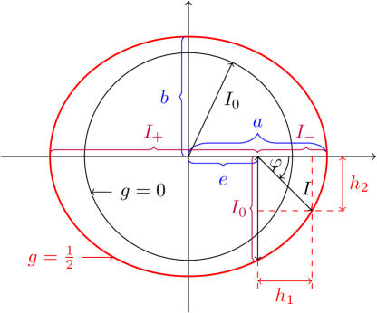
Figure 1: Phase space $\mathcal{S}_{\varphi,I}$: 1. Graph of the circular orbit $\{(\varphi\in[0,2\pi),I=I_{0}>0)\}$ generated by the periodic motion (6) of the ”orthodox” HO (in black). 2. Graph of the elliptical orbit $I(\varphi)=I_{0}/(1+g\,\cos\varphi)$ associated with the periodic motions (31) and (36) (in red, with g=1/2). Origin of the polar coordinates $(\varphi,I)$ here is the right focus. The meaning of the different letters with their related quantities and their historical names are described in the list (26)

The same holds for the hyperbola with the focus of the left branch as the origin for the polar coordinates:

Hyperbola,  $$g>1$$: (27)

• If $g>1$ the expression (25) describes a hyperbola of which we consider one branch only: the one open to the left. Its point of closest distance to the (inside) focus is $I_{0}/(1+g)$ where $\varphi=0$.

• semi-latus rectum: $I_{0}$,

• numerical eccentricity: $g$,

• linear eccentricity: $e=gI_{0}/(g^{2}-1)$
  (2$e$ is the distance of the 2 foci),

• major and minor semi-axis:
  $a=I_{0}/(g^{2}-1),\,\,\,b=I_{0}/(g^{2}-1)^{1/2}$,

• The two angles $\varphi_{\infty}(i),\,i=1,2$ characterizing the asymptotes are determined by $\cos\varphi_{\infty}(i)=-1/g,\,\varphi_{\infty}(1)\in(\pi/2,\pi)\text{ and }\varphi_{\infty}(2)\in(\pi,\pi+3\pi/2)$.

Parabola,  $$g=1$$: (28)

This simple case can be treated in the same way as the two others above.

Obviously, the orbits of the last two cases extend to infinity.

II.1.3 Time evolution

Ellipse
The time evolution follows from Eq. (19):

$$\int_{\varphi_{0}}^{\varphi}\frac{d\vartheta}{1+g\,\cos\vartheta}=\omega\,(t-t_{0}).$$ (29)

For $g<1$ wir get Gradshteyn and Ryzhik (1965) with $\varphi_{0}=0$ for $t_{0}=0$:

$$\sqrt{1-g^{2}}\,\omega\,t=2\arctan\left[\sqrt{\frac{1-g}{1+g}}\tan(\varphi/2)\right],$$ (30)

or

$$\tan[\varphi(t)/2]=\sqrt{\frac{1+g}{1-g}}\tan(\sqrt{1-g^{2}}\,\omega\,t/2).$$ (31)

Thus, the interaction $g\,h_{1}(\varphi,I)$ leads to an effective redshifted angular frequency

$$\omega_{g}=\sqrt{1-g^{2}}\,\omega,$$ (32)

with a branch point for $g^{2}\to 1$.

It follows from Eq. (30) that the time $t(\pi/2)$ needed to pass from $\varphi=0$ to $\varphi=\pi/2$ is given by

$$\omega_{g}\,t(\pi/2)=2\arctan\sqrt{\frac{1-g}{1+g}}=\arccos g.$$ (33)

At that time $I[t(\pi/2)]=I_{0}$ (see Eq. (25)).

The time needed to pass from $\varphi=0$ to $\varphi=\pi$ is

$$\omega_{g}\,t(\pi)=\pi.$$ (34)

Here we have $I[t(\pi)]=I_{0}/(1-g)$ (“aphelion”).

For reasons of symmetry of the ellipse we get from Eq. (34) for one period

$$\omega_{g}\,T_{g;2\pi}=2\pi,\,\,T_{g;2\pi}=\frac{2\pi}{\omega\sqrt{1-g^{2}}}.$$ (35)

Thus, $1/\sqrt{1-g^{2}}$ is a kind of “refractive index”.

Once the time evolution $\varphi(t)$ is known that of $I(t)$ can be obtained from the orbit equation (25). Using the relation $\cos\varphi=1-\tan^{2}(\varphi/2)/[1+\tan^{2}(\varphi/2)]$ one obtains

$$I(t)=\frac{I_{0}}{1-g^{2}}(1-g\cos[\omega_{g}t]),$$ (36)

which again gives the relations (33), (34) and (35).

The above results may be looked at as follows: For vanishing $g$ we have on $\mathcal{S}_{\varphi,I}$ a clockwise periodic motion with frequency $\omega$ on a circle of radius $I_{0}$. Adding the interaction $g\,h_{1}(\varphi,I),\,0\leq g<1,$ deformes the circle into an ellipse with semi-latus rectum $I_{0}$ and numerical eccentricity $g$. In addition the original angular frequency $\omega$ of the periodic motion is reduced to $\omega_{g}=\sqrt{1-g^{2}}\,\omega$.

Pictorially speaking we start with a “circularly polarized” motion ($g=0$) which encounters a medium ($0<g<1$) which induces an “elliptical polarization” and reduces the original angular frequency $\omega$!

Hyperbola
As before the time evolution can be calculated from Eq. (19), the integration of which now gives Gradshteyn and Ryzhik (1965)

$$\tan[\varphi(t)/2]=\sqrt{\frac{g+1}{g-1}}\tanh[\sqrt{g^{2}-1}\,\omega\,t/2].$$ (37)

Parabola
Finally, the time evolution for the parabola ($g=1$) is given by gra (a)

$$\tan[\varphi(t)/2]=\omega\,t\,.$$ (38)

II.2 Orbits on $\mathcal{S}_{q,p}$

Using the mappings (1) the orbit equation (25) in $\mathcal{S}_{\varphi,I}$ can be mapped onto $\mathcal{S}_{q,p}$, where it has the parametrization

$$q_{g}(\varphi)= \sqrt{\frac{2I_{0}}{m\omega(1+g\cos\varphi)}}\cos\varphi$$ (39)

$$p_{g}(\varphi)= -\sqrt{\frac{2m\omega I_{0}}{1+g\cos\varphi}}\sin\varphi.$$ (40)

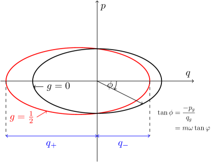
Figure 2: Phase space $\mathcal{S}_{q,p}$: 1. Graph of the “orthodox” elliptical orbit generated by the usual HO (in black) 2. Graph of the image of the (red) ellipse in Fig. 1 as described by Eqs. (39) and (40) (in red). Here $\phi$ is the polar angle on $\mathcal{S}_{q,p}$ and $\varphi$ the polar angle on $\mathcal{S}_{\varphi,I}$.

It implies

$$H(q_{g},p_{g}) =\frac{p_{g}^{2}}{2m}+\frac{1}{2}m\omega^{2}\,q_{g}^{2}$$ (41)

$$=\omega\,I=\frac{\omega\,I_{0}}{1+g\,\cos\varphi},$$

$$-\frac{p_{g}}{q_{g}}\equiv\tan\phi=m\,\omega\tan\varphi.$$ (42)

and

$$\cos\varphi=\frac{\sqrt{m/2}\;\omega\,q_{g}}{\sqrt{H(q_{g},p_{g})}}=\pm\sqrt{V(q_{g},p_{g})/H(q_{g},p_{g})}.$$ (43)

Inserting the last expression into Eq. (41) yields a 4th order equation in $q_{g}$ and $p_{g}$ for the orbit described by Eqs. (39) and (40):

$$H(q_{g},p_{g})\pm g\,\sqrt{V(q_{g},p_{g})\,H(q_{g},p_{g})}=\omega\,I_{0},$$ (44)

$$[H(q_{g},p_{g})-\omega\,I_{0}]^{2}=g^{2}\,V(q_{g},p_{g})\,H(q_{g},p_{g}).$$

For $g=0$ this is reduced to the usual orbit ellipse of the HO on $\mathcal{S}_{q,p}$ (See Fig. 2):

$$\frac{p_{g=0}^{2}}{2m}+\frac{1}{2}m\omega^{2}\,q_{g=0}^{2}=E_{0}=\omega I_{0}=\text{const. }$$ (45)

The functions (39) and (40) have the special values

$$q_{g}(0)\equiv q_{-} =\sqrt{\frac{2I_{0}}{m\omega(1+g)}},\,\,\,p_{g}(0)=0,$$ (46)

$$q_{g}(\pi/2) =0,\,\,~{}~{}p_{g}(\pi/2)=-\sqrt{2m\omega I_{0}},$$

$$q_{g}(\pi)\equiv q_{+} =-\sqrt{\frac{2I_{0}}{m\omega(1-g)}},\,\,\,p_{g}(\pi)=0,$$

$$q_{g}(3\pi/2) =0,\,\,~{}~{}p_{g}(3\pi/2)=\sqrt{2m\omega I_{0}}.$$

Note that the 4th order figure defined by Eq. (44) is symmetric with respect to the $q$-axis, but no longer symmetric with respect to the $p$-axis (see Fig. 2). Maximum and minimum of $p_{g}(\varphi)$ are given by the angles $\varphi_{\pm}$, which obey

$$\cos\varphi_{\pm}=-(1-\sqrt{1-g^{2}})/g.$$ (47)

II.3 The frequency $\omega$ as an external field

According to Eq. (3) the Hamiltonian of the HO on $\mathcal{S}_{\varphi,I}$ has the simple form

$$H(\varphi,I)=\omega\,I,$$ (48)

where the frequency $\omega$ appears as a parameter multiplying the basic action variable $I$.

That parameter $\omega$ may also be considered as an external “field” which can be “manipulated” from outside, e.g., as a function $\omega(t)$ of time $t$. The solution of Eq. (4) then is

$$\varphi(t)-\varphi(t_{0})=\int_{t_{0}}^{t}d\tau\,\omega(\tau).$$ (49)

Note that the Hamiltonian (48) is independent of $\varphi$ and therefore $\dot{I}=-\partial_{\varphi}H(\varphi,I)=0$, even if $\omega=\omega(t)$! Thus, the action variable $I$ is still conserved on $\mathcal{S}_{\varphi,I}$, but the energy $E=\omega(t)\,I$ is not! A possible interesting example for applications is a time dependent angular frequency of the form

$$\omega(t)=\omega_{0}+\lambda\sin(\rho t),\;|\lambda|<\omega_{0}.$$ (50)

   In the present context it is also appropriate to briefly recall the so-called “adiabatic invariance” bor ; Born and Fock (1928); Landau and Lifshitz (1969); Thirring (2002); Arnold et al. (2006) of the action variable I: If energy $E(\lambda)$ and frequency $\omega(\lambda)$ of a periodic motion with period $T$ depend on a slowly varying parameter $\lambda$ ( $T\,d\lambda/dt\ll\lambda$), then $I=E(\lambda)/\omega(\lambda)$ remains constant if $\lambda$ varies.

In the following discussions on the “non-orthodox” quantum mechanics of the HO it is essential to differentiate between the quantum counterparts of the action variable $I$ and the Hamilton function $H$, the generator of time evolution.

For a given “binding” potential $V(q)$ the angular frequency $\omega$ is generally defined as one half of the 2nd derivative of $V(q)$ at its (local) minimum $q=q_{0}$ : $\omega=(1/2)\,d^{2}V(q)/dq^{2}_{|q=q_{0}}$.

III Quantum mechanics of the phase space $\mathcal{S}_{\varphi,I}$

III.1 Basics: self-adjoint representations of the
three Lie algebra generators $K_{j}$ of
the symplectic group $Sp(2,\mathbb{R})$

The quantization of the global “coordinates” $h_{j}$ from Eq. (14) is implemented by reinterpreting them as self-adjoint operators in a given Hilbert space ka1 (c),

$$h_{j}\to K_{j}=\hbar\,\tilde{K}_{j}\,$$ (51)

which obey the associated Lie algebra (16):

$$[\tilde{K}_{0},\,\tilde{K}_{1}]=i\,\tilde{K}_{2}\,, ~{}~{}[\tilde{K}_{0},\,\tilde{K}_{2}]=-i\,\tilde{K}_{1}\,,$$ (52)

$$[\tilde{K}_{1},\,\tilde{K}_{2}] =-i\,\tilde{K}_{0}\,.$$ (53)

(Quantities $\tilde{A}$ with a ”tilde”, here and in the following, are considered to be dimensionless).

The three self-adjoint operators $\tilde{K}_{j}$ can be obtained as Lie algbra generators of irreducible unitary representations of the corresponding groups $SO^{\uparrow}(1,2)$, $Sp(2,\mathbb{R})$ (the latter being isomorphic to the groups $SL(2,\mathbb{R})$ and $SU(1,1)$) or of one of their infinitely many covering groups kas (c).

As $\tilde{K}_{0}$ is the generator of the maximal compact abelian subgroup $U(1)$, its eigenstates may be used as a Hilbert space basis (here formally in Dirac’s notation, explicit examples will be discussed later):

$$\tilde{K}_{0}|b,\,n\rangle=(n+b)\,|b,\,n\rangle\,,$$

where $b$ is some real number $\in(0,1)$ (“Bargmann index” Bargmann (1947)) and $n=0,1,2,\ldots$. This central result can be derived as follows

The operators

$$~{}\tilde{K}_{\pm}= \tilde{K}_{1}\pm i\,\tilde{K}_{2}\,,$$ (54)

$$K_{1}=\frac{1}{2}(\tilde{K}_{+}+\tilde{K}_{-}),\,K_{2}=\frac{1}{2i}(\tilde{K}_{+}-\tilde{K}_{-}),$$ (55)

obey the relations

$$[\tilde{K}_{0},\,\tilde{K}_{+}]=\tilde{K}_{+}\,, ~{}~{}[\tilde{K}_{0},\,\tilde{K}_{-}]=-\tilde{K}_{-}\,,$$ (56)

$$[\tilde{K}_{+},\,\tilde{K}_{-}] =-2\tilde{K}_{0}\,.$$ (57)

They are raising and lowering operators:

$$\tilde{K}_{+}|b,\,n\rangle =[(2b+n)(n+1)]^{1/2}\,|b,\,n+1\rangle\,,$$ (58)

$$\tilde{K}_{-}|b,\,n\rangle =[(2b+n-1)n]^{1/2}\,|b,\,n-1\rangle\,.$$ (59)

The relations (58) and (59) are derived under the assumptions that there exists a state $|b,0\rangle$ such that

$$\tilde{K}_{0}|b,0\rangle=b\,|b,0\rangle\,,~{}~{}~{}\tilde{K}_{-}|b,0\rangle=0,~{}b\in[1,0).$$ (60)

Eq. (58) implies

$$|b,n\rangle= \frac{1}{\sqrt{(2b)_{n}\,n!}}(\tilde{K}_{+})^{n}|b,0\rangle,$$ (61)

$$(2b)_{n}=2b(2b+1)\cdots(2b+n-1)$$

$$~{}~{}~{}~{}~{}~{}~{}=\Gamma(2b+n)/\Gamma(2b).$$

It then follows that

$$\tilde{K}_{0}\,|b,n\rangle=(n+b)\,|b,n\rangle\,,\,n=0,1,\ldots;~{}~{}1>b>0\,.$$ (62)

This is the so-called “positive discrete series” $D_{b}^{(+)}$ among the different types of possible irreducible unitary representations of $Sp(2,\mathbb{R})$ Bargmann (1947); kas (c) The Bargmann index $b$ - called “B-index” in the following - characterizes an irreducible unitary representation (IUR) $D_{b}^{(+)}$.

The Casimir operator

$$\mathfrak{C} =\tilde{K}_{1}^{2}+\tilde{K}_{2}^{2}-\tilde{K}_{0}^{2}$$ (63)

$$=\tilde{K}_{+}\tilde{K}_{-}-\tilde{K}_{0}\,(\tilde{K}_{0}-1)$$

$$=\tilde{K}_{-}\tilde{K}_{+}-\tilde{K}_{0}\,(\tilde{K}_{0}+1)$$

of the IUR $D_{b}^{(+)}$ has the value

$$\mathfrak{C}=b(1-b){\bf 1}\,.$$ (64)

This means that the “classical Pythagoras” (15) is violated quantum mechanically for $b\neq 1$, e.g. in the case of the usual HO with $b=1/2$!

The Group $SO^{\uparrow}(1,2)$ has infinitely many covering groups because its compact subgroup $O(2)\cong S^{1}\cong U(1)$ is infinitely connected!

Let us denote the $s$-fold covering by

$$SO^{\uparrow}_{[s]}(1,2)\,,\,s=1,2,\ldots\,.$$ (65)

Its irreducible unitary representations $D_{b}^{(+)}$ have the indices

$$b=\frac{r}{s}\,,~{}r=1,2,\ldots,s-1\,.$$ (66)

This means that $b_{min}=1/s$ can be arbitrarily small $>0$ if $s$ is large enough!
The 2-fold coverings

$$Sp(2,\mathbb{R})=SL(2,\mathbb{R})\,\cong SU(1,1)$$ (67)

have $b=1/2$.

The results above imply that the $(\varphi,I)$-Hamiltonian

$$H(\varphi,I)\to H_{osc}(K)=\omega\,K_{0}\,,~{}~{}K=\hbar\,(\tilde{K}_{0},\tilde{K}_{1},\tilde{K}_{2})\,$$ (68)

can have the $b$-dependent spectra

$$E_{b,\,n}(\varphi,I)=\hbar\,\omega\,(n+b)\,,\,n=0,1,\ldots\,;~{}~{}1>b>0,$$ (69)

As this result is due to the properties of the symplectic group $Sp(2,\mathbb{R})$, especially its compact subgroup $U(1)\cong O(2)$, we call it the “symplectic spectrum” of the HO, and the conventional special case $b=1/2$ as its “orthodox” one.

Because of the relations (55), (58) and (59) one has

$$\langle b,n|\tilde{K}_{j}|b,n\rangle=0\,,~{}j=1,2,$$ (70)

implying for the mean square deviations

$$(\Delta\tilde{K}_{j})^{2}_{b,n}=\frac{1}{2}(n^{2}+2nb+b)\,,~{}j=1,2,$$ (71)

so that

$$(\Delta\tilde{K}_{1})_{b,n}\,(\Delta\tilde{K}_{2})_{b,n}=\frac{1}{2}(n^{2}+2bn+b)\,,$$ (72)

$$(\Delta\tilde{K}_{1})_{b,n=0}\,(\Delta\tilde{K}_{2})_{b,n=0}=\frac{b}{2}\,.$$ (73)

The last relation shows that $b\to 0$ is a kind of classical limit in the angle-action framework!

III.2 Time evolution

III.2.1 Heisenberg picture

The appearence of covering groups (65) has a natural physical background: Take the time dependence of the angle $\varphi(t)=\omega\,t$ in Eq. (6) (with $t_{0}=0,\varphi_{0}=0$): In general the system will not stop after covering a circle just once, $\omega\,T_{1}=2\pi$, but will circle the origin, say, at least $s$ times, $\omega\,T_{s}=2\pi\,s$, where $s\in\mathbb{N}$ can be arbitrarily large.

In the following the dimensionless time variable

$$\tilde{t}=\omega\,t$$ (74)

will be used. It is an angle variable.

The unitary time evolution operator is given by

$$U(\tilde{t})=e^{-i\,\tilde{K_{0}}\,\tilde{t}}\,,~{}~{}\tilde{K}_{0}=N+b\bf{1}\,,$$ (75)

where the number operator $N$ can be considered a function of the operators $\tilde{K}_{j},\,j=0,1,2$, as will be shown below.

The unitary operator (75) implies the usual Heisenberg Eqs. of motion:

$$U(-\tilde{t})\,\tilde{K}_{+}\,U(\tilde{t}) =e^{-i\tilde{t}}\tilde{K}_{+},$$ (76)

$$U(-\tilde{t})\,\tilde{K}_{-}\,U(\tilde{t}) =e^{+i\tilde{t}}\tilde{K}_{-},$$ (77)

$$U(-\tilde{t})\,\tilde{K}_{1}\,U(\tilde{t}) =\cos\tilde{t}\,\tilde{K}_{1}+\sin\tilde{t}\,\tilde{K}_{2},$$ (78)

$$U(-\tilde{t})\,\tilde{K}_{2}\,U(\tilde{t}) =-\sin\tilde{t}\,\tilde{K}_{1}+\cos\tilde{t}\,\tilde{K}_{2}.$$ (79)

For $\tilde{t}=2\pi$ the operator (75) becomes

$$U(\tilde{t}=2\pi)=e^{-2\pi ib}{\bf 1}\,.$$ (80)

If

$$b=r/s\,,~{}r,s\in\mathbb{N},\,r<s\text{ and divisor free},$$ (81)

this implies for $SO^{\uparrow}_{[s]}(1,2)$:

$$U(\tilde{t}=s\,2\pi)={\bf 1}\,.$$ (82)

The ground state $|b,0\rangle$ has the time evolution

$$U(\tilde{t})\,|b,0\rangle=e^{-i\,b\,\tilde{t}}\,|b,0\rangle\,,$$ (83)

with the associated time period

$$T_{2\pi,b}=\frac{2\pi}{\omega_{b}},\;\;\omega_{b}\equiv b\,\omega\,,$$ (84)

which can become arbitrarily large for $b=1/s,\,s\to\infty$. Symbolically speaking: $1/b$ is a kind of refraction index $n$.

Whereas $\tilde{K}_{0}$ generates rotations and time evolutions by performing many phase rotations, the operators $\tilde{K}_{1}$ and $\tilde{K}_{2}$ generate special “Lorentz” transformations (“boosts”) in directions 1 and 2, respectively ka1 (d):

With

$$U(w)= e^{(w/2)\tilde{K}_{+}-(w^{\ast}/2)\tilde{K}_{-}}=e^{i\,w_{2}\tilde{K}_{1}+i\,w_{1}\tilde{K}_{2}},$$ (85)

$$w=w_{1}+i\,w_{2}=|w|e^{i\theta}$$

one obtains

$$U(-w)\vec{\tilde{K}}U(w)= \vec{\tilde{K}}(\cosh|w|-1)(\vec{n}\cdot\vec{\tilde{K}})\cdot\vec{n}$$ (86)

$$+\sinh|w|\,\vec{n}\,\tilde{K}_{0},$$

$$U(-w)\tilde{K}_{0}U(w)= \cosh|w|\tilde{K}_{0}+\sinh|w|(\vec{n}\cdot\vec{\tilde{K}}),$$ (87)

$$\vec{\tilde{K}}=(\tilde{K}_{1},\tilde{K}_{2}),\;\vec{n}=(\cos\theta,-\sin\theta).$$

Eqs. (86) and (87) describe a Lorentz “boost” in direction $\vec{n}$.

III.2.2 Schrödinger Picture

If $|b;t_{0}\rangle$ is a state vector of the Hilbert space associated with the B-index $b$ at time $t_{0}$, then - according to the unitary time evolution (75) - we have at time $t$:

$$|b;t\rangle=U(t-t_{0})|b;t_{0}\rangle=e^{-i\omega K_{0}(t-t_{0})/\hbar}|b;t_{0}\rangle,$$ (88)

which implies

$$\frac{\hbar}{i}\partial_{t}|b;t\rangle=\omega K_{0}|b;t\rangle,~{}K_{0}=\hbar\tilde{K}_{0}.$$ (89)

For a representation

$$|b;t\rangle=\sum_{n=0}^{\infty}c_{n}(t)|b,n\rangle$$ (90)

we get from Eq. (88), with $t_{0}=0$,

$$c_{n}(t)=e^{-i\omega(n+b)t},$$ (91)

so that

$$|b;t\rangle=e^{-ib\,\omega t}\sum_{n=0}^{\infty}e^{-i\,n\,\omega t}|b,n\rangle.$$ (92)

III.3 Relationship between the operators $\tilde{K}_{j}$
and the conventional operators $Q$ and $P$

The relations (1) expressed in terms of the functions $h_{j}(\varphi,I)$ from Eqs. (14) take the form

$$q(\varphi,I) =\sqrt{\frac{2}{m\,\omega}}\,\frac{h_{1}(\varphi,I)}{\sqrt{h_{0}(\varphi,I)}}\,,$$ (93)

$$p(\varphi,I) =\sqrt{2\,m\,\omega}\,\frac{h_{2}(\varphi,I)}{\sqrt{h_{0}(\varphi,I)}}\,.$$ (94)

There is a corresponding relationship at the operator level: Define the operators

$$A(K) =(\tilde{K}_{0}+b)^{-1/2}\tilde{K}_{-},$$ (95)

$$A^{\dagger}(K) =\tilde{K}_{+}(\tilde{K}_{0}+b)^{-1/2}.$$ (96)

According to Eqs. (62), (58) and (59) they act on the number states $|b,n\rangle$ as

$$A^{\dagger}\,|b,n\rangle =\sqrt{n+1}\,|b,n+1\rangle,$$ (97)

$$A\,|b,\,n\rangle =\sqrt{n}\,|b,n-1\rangle,$$ (98)

$$\,n=0,1,\ldots\,.$$

This means

$$[A,\,A^{\dagger}]={\bf 1}\,~{}~{}\forall~{}D_{b}^{(+)},$$ (99)

independent of the value of $b$ !

Thus, the composite operators $A(K)$ and $A^{\dagger}(K)$ are the usual Fock space annihilation and creation operators for all $b$ and independent of $b$ !

Note that the denominator in Eqs. (95) and (96) is well-defined, because $\tilde{K}_{0}$ is a positive definite operator and $b$ a positive number for each representation of the series $D^{(+)}_{b}$.

The quantum mechanical position and momentum operators $Q$ and $P$ can now be defined as usual:

$$Q=Q(K)= \,\frac{\lambda_{0}}{\sqrt{2}}\,[A^{\dagger}(K)+A(K)],$$ (100)

$$P=P(K)= \,\frac{i\,\hbar}{\sqrt{2}\,\lambda_{0}}\,[A^{\dagger}(K)-A(K],$$ (101)

$$\,\lambda_{0}=\sqrt{\hbar/(m\,\omega)},$$ (102)

where $\lambda_{0}$ has the dimension of a length.

The $(q,p)$-Hamilton operator

$$H(Q,P)=\, \frac{1}{2m}P^{2}(K)+\frac{1}{2}m\,\omega^{2}Q^{2}(K)$$ (103)

$$=\, \hbar\,\omega(N(K)+\frac{1}{2}{\bf 1}),$$

$$\,N(K)=A^{\dagger}(K)A(K)$$ (104)

$$~{}~{}~{}~{}~{}~{}~{}~{}=\tilde{K}_{+}(\tilde{K}_{0}+b)^{-1}\tilde{K}_{-}$$

has the usual “orthodox” spectrum $E_{n}=\hbar\omega(n+1/2)$ !

Thus, it turns out that the quantum mechanics associated with the phase space $\mathcal{S}_{\varphi,I}$ is rather more subtle than the one associated with $\mathcal{S}_{q,p}$ and that those subtleties get lost if one passes from the $(\varphi,I)$-case to the $(q,p)$-case!

As the creation and annihilation operators $A^{\dagger}$ $A$ with their ($b$-independent) defining properties (97), (98) and (99) are essential building blocks for many quantum systems, that loss of $b$-dependent subtleties may in turn lead to a corresponding loss of physical insights. The big question is: Did nature implement those subtleties?

The time evolution of the composite operators (100) and (101) is the usual one. It follows from the relations (76) and (79):

$$U(-\tilde{t})\,\tilde{Q}\,U(\tilde{t})= \cos\tilde{t}\,\tilde{Q}+\sin\tilde{t}\,\tilde{P}\,,$$ (105)

$$U(-\tilde{t})\,\tilde{P}\,U(\tilde{t})= -\sin\tilde{t}\,\tilde{Q}+\cos\tilde{t}\,\tilde{P}\,.$$ (106)

III.4 The model $H=\hbar\,\omega(\tilde{K}_{0}+g\,\tilde{K}_{1})$

III.4.1 Transition matrix elements with respect to the number states in 1st order

The quantum mechanical counterpart of the classical Hamiltonian (18) is the operator

$$H(K)=\hbar\,\omega\,\tilde{C}_{g}(K),\,\tilde{C}_{g}(K)=\tilde{K}_{0}+g\,\tilde{K}_{1},\,g\geq 0\,.$$ (107)

Before discussing a special explicit choice for the operators $\tilde{K}_{j}$, their associated Hilbert space and the exact eigenfunctions of the Hamiltonian (107) we mention the values of the (formal) 1st order matrix elements

$$\langle b,m|\tilde{C}_{g}(K)|b,n\rangle,\;m,n=0,1,2,\ldots$$ (108)

From the relations (55), (58) and (59) we get for $m\neq n$ (the case $m=n$ appears trivial, but that is only so in 1st order. It follows from the exact solution - discussed below - that the 2nd order $g^{2}$ and higher ones contribute):

$$\langle b,m|\tilde{C}_{g}(K)|b,n\rangle= \frac{g}{2}\langle b,m|(\tilde{K}_{+}+\tilde{K}_{-})|b,n\rangle$$ (109)

$$= \frac{g}{2}[(2b+n)(n+1)]^{1/2}\,\delta_{m(n+1)}$$

$$+ \frac{g}{2}[(2b+n-1)n]^{1/2}\,\delta_{m(n-1)}.$$

Thus, we have the selection rule

$$\Delta n=\pm 1,$$ (110)

for the Hamiltonian (107), the same as, e.g., for vibrational (electric dipole) transitions of diatomic molecules her (b)!

Examples:

$$\langle b,m=0|\tilde{C}_{g}(K)|b,n=1\rangle= \frac{g}{2}\sqrt{2b},$$ (111)

$$\langle b,m=2|\tilde{C}_{g}(K)|b.n=1\rangle= \frac{g}{2}\sqrt{2(2b+1)},$$ (112)

$$\langle b,m=n_{0}-1|\tilde{C}_{g}(K)|b,n_{0}\rangle= \frac{g}{2}\sqrt{n_{0}(2b+n_{0}-1)},$$ (113)

$$\langle b,m=n_{0}+1|\tilde{C}_{g}(K)|b,n_{0}\rangle= \frac{g}{2}\sqrt{(n_{0}+1)(2b+n_{0})}$$ (114)

Eq. (111) shows that the associated transition probability for $0\leftrightarrow 1$ is proportional to $b$.

III.4.2 Exact eigenvalues of $\tilde{C}_{g}(K)$

It follows from the explicit Hilbert space calculations in Ch. III.E and in Appendix A that the operator $\tilde{C}_{g}(K)$ has the exact eigenvalues

$$\tilde{c}_{g,b;n}=(n+b)\sqrt{1-g^{2}},~{}n=0,1,\ldots,$$ (115)

so that the Hamiltonian (107) has the the eigenvalues

$$\tilde{E}_{g,b;n}=\hbar\omega_{g}(n+b),~{}n=0,1,\ldots,~{}\omega_{g}=\sqrt{1-g^{2}}\omega,$$ (116)

which reflects the (”redshifted”) frequency reduction (32) of the classical motions in Ch. II.

III.5 Explicit Hilbert spaces for $\tilde{K}_{j},j=0,1,2$ and $\tilde{C}_{g}(K)=\tilde{K}_{0}+g\tilde{K}_{1}$, spectra and eigenfunctions

Several explicit Hilbert spaces for concrete irreducible unitary representations of the group $SO^{\uparrow}(1,2)$, its twofold covering the symplectic group $Sp(2,\mathbb{R})$ (or the isomorphic ones $SU(1,1)$ and $SL(2,\mathbb{R}$) and of all other covering groups as well have been discussed in the literature Bargmann (1947); P. J. Sally (1967); Vilenkin (1968); P. J. Sally (1970); Boyer and Wolf (1975); ka1 (e).

The associated self-adjoint Lie algebra generators $\tilde{K}_{j}$ all obey the same commutation relations (10). The representation spaces include Hardy spaces on the unit circle $\mathbb{S}^{1}$, Hilbert spaces of holomorphic functions on the unit disc $\mathbb{D}=\{\lambda\in\mathbb{C},|\lambda|<1\}$ and also Hilbert spaces on the positive real line $\mathbb{R}^{+}_{0}=\{x\in\mathbb{R},x\geq 0\}$. We shall present Hardy space related Hilbert spaces for $b\in(0,1)$ here and discuss corresponding Hilbert spaces on $\mathbb{R}^{+}_{0}$ in Appendix A: Hardy spaces on the unit circle are closely related to the variable angle, whereas Hardy Hilbert spaces on $\mathbb{R}^{+}_{0}$ are associated with the action variable $I$.

The following discussion follows closely those of Secs. 7.1 and 7.2 of Ref. Kastrup (2007). Mathematical details like, e.g. questions concerning the convergence of series or integrals, will be ignored in the following! The associated justification can be found in the mathematical literature quoted above.

III.5.1 Hardy space on the unit circle

A “Hardy space” $H^{2}_{+}(\mathbb{S}^{1},d\vartheta)$ is a closed subspace of the usual Hilbert space $L^{2}(\mathbb{S}^{1},d\vartheta)$ on the unit circle $\mathbb{S}^{1}$ with the scalar product

$$(f_{2},f_{1})=\frac{1}{2\pi}\,\int_{S^{1}}d\vartheta\,f_{2}^{*}(\vartheta)f_{1}(\vartheta)\,,$$ (117)

and the orthonormal basis

$$e_{n}(\vartheta)=e^{i\,n\,\vartheta}\,,~{}~{}n\in\mathbb{Z}\,.$$ (118)

The associated Hardy subspace $H^{2}_{+}(\mathbb{S}^{1},\,d\vartheta)$ is spanned by the basis consisting of the elements with non-negative $n$, namely

$$e_{n}(\vartheta)=e^{i\,n\,\vartheta}\,,~{}~{}n=0,1,2,\cdots\,.$$ (119)

If we have two Fourier series $\in H^{2}_{+}(\mathbb{S}^{1}\,,d\vartheta)$,

$$f_{1}(\vartheta)=\sum_{n=0}^{\infty}c_{n,1}\,e^{i\,n\,\vartheta}\,,~{}~{}f_{2}(\vartheta)=\sum_{n=0}^{\infty}c_{n,2}\,e^{i\,n\,\vartheta}\,,$$ (120)

they have the scalar product

$$(f_{2},f_{1})_{+}=\frac{1}{2\pi}\int_{S^{1}}d\vartheta\,f^{*}_{2}(\vartheta)f_{1}(\vartheta)=\sum_{n=0}^{\infty}c^{*}_{n,2}\,c_{n,1}$$ (121)

and obey the boundary condition

$$f_{j}(\vartheta+2\pi)=f_{j}(\vartheta),\;j=1,2.$$ (122)

The coefficients $c_{n,j}$ are given by

$$c_{n.j}=(e_{n},f_{j})_{+}.$$ (123)

$Sp(2,\mathbb{R})$ Lie algebra generators are

$$\tilde{K}_{0} = \frac{1}{i}\partial_{\vartheta}+\frac{1}{2}\,,$$ (124)

$$\tilde{K}_{+} = e^{i\,\vartheta}\,(\frac{1}{i}\partial_{\vartheta}+1),$$ (125)

$$\tilde{K}_{-} = e^{-i\,\vartheta}\,\frac{1}{i}\partial_{\vartheta}.$$ (126)

Thus, the Hardy space with the basis (119) provides a Hilbert space for the conventional HO with the spectrum $\{n+1/2$} and the operators (124)-(126) act on the basis (119) as

$$\tilde{K}_{0}\,e_{n}(\vartheta) = (n+\frac{1}{2})\,e_{n}(\vartheta)\,,$$ (127)

$$\tilde{K}_{+}\,e_{n}(\vartheta) = (n+1)\,e_{n+1}(\vartheta)\,,$$ (128)

$$\tilde{K}_{-}\,e_{n}(\vartheta) = n\,e_{n-1}(\vartheta)\,,$$ (129)

which are special cases of the relations (62), (58) and (59) with $b=1/2$. Note that the ground state here is given by $e_{n=0}(\vartheta)=1$.

A possible generalization of the case $b=1/2$ for $b\in(0,1)$ within the same Hilbert space as above can be obtained Bojowald and Strobl (2000); hol by inspection of the relations (62), (58) and (59):

$$\tilde{K}_{0} =N+b,~{}~{}N=\frac{1}{i}\partial_{\vartheta},$$ (130)

$$\tilde{K}_{+} =e^{i\vartheta}[(N+2b)(N+1)]^{1/2},$$ (131)

$$\tilde{K}_{-} =[(N+2b)(N+1)]^{1/2}e^{-i\vartheta}.$$ (132)

Applied to the basis (119) these operators have the correct properties.

Defining the self-adjoint operator

$$M_{b}(N) =+[(N+2b)(N+1)]^{1/2}=M_{b}^{\dagger},$$ (133)

$$=+[(\tilde{K}_{o}+b)(N+1)]^{1/2},$$

with

$$M_{b}(N)\,e^{in\vartheta}=+[(n+2b)(n+1)]^{1/2}\,e^{in\vartheta},$$ (134)

the operators (131) and (132) can be written as

$$\tilde{K}_{+}=(e^{i\vartheta}\,M_{b})\,,~{}~{}\tilde{K}_{-}=(M_{b}\,e^{-i\vartheta}).$$ (135)

III.5.2 Hardy space related Hilbert spaces for general $b\in(0,1]$

Another possible representation for the more general case $b\in(0,1)$ can be obtained by a generalization of the the scalar product (121):

Introducing on $H_{+}^{2}(\mathbb{S}^{1},d\vartheta)$ the positive definite (self-adjoint) operator $A_{b}$ by the action

$$A_{b}\,e_{n}(\vartheta)= \frac{n!}{(2b)_{n}}e_{n}(\vartheta),~{}n=0,1,\ldots\,,~{}b>0,$$ (136)

$$(a)_{n}=a\,(a+1)\,(a+2)\ldots(a+n-1)$$

$$~{}~{}~{}~{}~{}\;=\Gamma(a+n)/\Gamma(a),\,\,(a)_{n=0}=1,$$

one can define an additional scalar product for functions

$$f_{j}(\vartheta)=\sum_{n=0}^{\infty}c_{n,j}e_{n}(\vartheta)\,,~{}j=1,2,$$ (137)

by

$$(f_{2},f_{1})_{b,+}\equiv(f_{2},A_{b}\,f_{1})_{+}=\sum_{n=0}^{\infty}\frac{n!}{(2b)_{n}}\,c^{*}_{n,2}\,c_{n,1}\,,$$ (138)

so that

$$(e_{n},f_{1})_{b,+}=\frac{n!}{(2b)_{n}}\,c_{n,1}.$$ (139)

We denote the (Hardy space associated) Hilbert space with the scalar product (138) by $H^{2}_{b,+}(\mathbb{S}^{1},d\vartheta)$.

An orthonormal basis in this space is given by

$$\hat{e}_{b,n}(\vartheta)= \sqrt{\frac{(2b)_{n}}{n!}}\,e_{n}(\vartheta)\,,$$ (140)

$$(\hat{e}_{b,n_{2}},\hat{e}_{b,n_{1}})_{b,+}=\delta_{n_{2}n_{1}}.$$

Two series

$$f_{j}(\vartheta)=\sum_{n=0}^{\infty}a_{n,j}\,\hat{e}_{b,n}(\vartheta)\,,~{}j=1,2,$$ (141)

have the obvious scalar product

$$(f_{2},f_{1})_{b,+}= \sum_{n=0}^{\infty}a^{*}_{n,2}\,a_{n,1},$$ (142)

$$a_{n,1}= (\hat{e}_{b,n},f_{1})_{b,+}$$ (143)

It follows that for a given function $f(\vartheta)$ its expansion coefficients $c_{n}$ or $a_{n}$ with respect to $e_{n}$ or $e_{b,n}$ are related as follows

$$c_{n}=(e_{n},f)_{+}=\sqrt{\frac{n!}{(2b)_{n}}}\,(\hat{e}_{b,n},f)_{+}=\sqrt{\frac{n!}{(2b)_{n}}}\,a_{n}$$ (144)

As in general

$$(f,f)_{+}\neq(f,f)_{b,+},$$ (145)

one has to be careful in the case of quantum mechanical applications:

In a Hilbert space with scalar product $(f_{2},f_{1})$ one generally needs the normalization $(f,f)=1$ for the usual probability interpretations. If initially $(f,f)\neq 1$ one has to renormalize the state $f$: $f\to f/\sqrt{(f,f)}$. So, if, e.g. $(f,f)_{+}=1$ in inequality (145), one has to renormalize $f$ if one wants to determine transition probabilities and expectation values etc. with respect to (138).

In $H^{2}_{b,+}(\mathbb{S}^{1},d\vartheta)$ the generators $\tilde{K}_{j}$ have the form ka1 (c, e)

$$\tilde{K}_{0}= \frac{1}{i}\,\partial_{\vartheta}+b,$$ (146)

$$\tilde{K}_{+}= e^{i\,\vartheta}(\frac{1}{i}\partial_{\vartheta}+2b),$$ (147)

$$\tilde{K}_{-}= e^{-i\,\vartheta}\frac{1}{i}\partial_{\vartheta},$$ (148)

so that

$$\tilde{K}_{1}= \frac{1}{2}(\tilde{K}_{+}+\tilde{K}_{-})=\cos\vartheta\,\frac{1}{i}\partial_{\vartheta}+b\,e^{i\vartheta},$$ (149)

$$\tilde{K}_{2}= \frac{1}{2i}(\tilde{K}_{+}-\tilde{K}_{-})=\sin\vartheta\,\frac{1}{i}\partial_{\vartheta}-ib\,e^{i\vartheta}$$ (150)

$$= \tilde{K}_{1}(\vartheta-\pi/2).$$

The operators (147) and (148) have the correct actions (58) and (59) on the basis (140):

$$\tilde{K}_{0}\,\hat{e}_{b,n} = (n+b)\,\hat{e}_{b,n}\,,$$ (151)

$$\tilde{K}_{+}\,\hat{e}_{b,n} = \sqrt{(2b+n)(n+1)}\,\hat{e}_{b,n+1}\,,$$ (152)

$$\tilde{K}_{-}\,\hat{e}_{b,n} = \sqrt{(2b+n-1)n}\,\hat{e}_{b,n-1}\,.$$ (153)

The operators (147) and (148) are adjoint to each other only with respect to the scalar product (138), not with respect to (121). Their adjointness with respect to the scalar product (138) can be verified by taking two series (141) and showing that

$$(\tilde{K}_{-}f_{2},f_{1})_{b,+}=(f_{2},\tilde{K}_{+}f_{1})_{b,+}.$$ (154)

This relation implies the self-adjointness of the operators (149) and (150). Note that

$$(e_{n_{2}},\hat{e}_{b,n_{1}})_{+} =(\hat{e}_{b,n_{1}},e_{n_{2}})_{+}=\sqrt{\frac{(2b)_{n_{1}}}{n_{1}!}}\,\delta_{n_{2}\,n_{1}},$$ (155)

$$(e_{n_{2}},\hat{e}_{b,n_{1}})_{b,+} =(\hat{e}_{b,n_{1}},e_{n_{2}})_{b,+}=\sqrt{\frac{n_{1}!}{(2b)_{n_{1}}}}\,\delta_{n_{2}\,n_{1}},$$ (156)

$$(\hat{e}_{b,n_{2}},\hat{e}_{b,n_{1}})_{+} =\frac{(2b)_{n_{1}}}{n_{1}!}\,\delta_{n_{2}\,n_{1}},$$ (157)

$$(e_{n_{1}},e_{n_{2}})_{b,+} =\frac{n_{1}!}{(2b)_{n_{1}}}\,\delta_{n_{2}\,n_{1}}\,.$$ (158)

The Fock space ladder operators $A$ and $A^{\dagger}$ associated with the Lie algebra generators (146)-(148) are given according to Eqs. (95).

The so-called “reproducing kernel” on $H^{2}_{b,+}$ is given by the “completeness” relation

$$\hat{A}_{b}(\vartheta_{2}-\vartheta_{1})= \sum_{n=0}^{\infty}\hat{e}^{*}_{b,n}(\vartheta_{2})\,\hat{e}_{b,n}(\vartheta_{1})$$ (159)

$$=[1-e^{i\,(\vartheta_{1}-\vartheta_{2})}]^{-2b}= \hat{A}_{b}^{*}(\vartheta_{1}-\vartheta_{2})\,,$$ (160)

where the identity

$$\frac{(a)_{n}}{n!}=(-1)^{n}{-a\choose n}$$ (161)

has been used. According to the relations (155) – (158) the kernel (159) has the properties

$$\frac{1}{2\pi}\int_{\mathbb{S}^{1}}d\vartheta_{2}\hat{A}_{b}(\vartheta_{2}-\vartheta_{1})\hat{e}_{b,m}(\vartheta_{2})=\hat{e}_{b,m}(\vartheta_{1}),$$ (162)

or, written more formally in terms of the scalar product (138)

$$(\hat{A}_{b}(1,2),\,\hat{e}_{b,m}(2))_{b,+} =\hat{e}_{b,m}(\vartheta_{1}),$$ (163)

$$(\hat{A}_{b}(1,2),\,\hat{e}_{b,m}(2))_{+} =\frac{(2b)_{m}}{m!}\,\hat{e}_{b,m}(\vartheta_{1}),$$ (164)

$$(\hat{A}_{b}(1,2),\,e_{m}(2))_{b,+} =\sqrt{\frac{m!}{(2b)_{m}}}\,\hat{e}_{b,m}(\vartheta_{1})=e_{m}(\vartheta_{1}),$$ (165)

$$(\hat{A}_{b}(1,2),\,e_{m}(2))_{+} =\sqrt{\frac{(2b)_{m}}{m!}}\,\hat{e}_{b,m}(\vartheta_{1})$$ (166)

$$=\frac{(2b)_{m}}{m!}\,e_{m}(\vartheta_{1}).$$

The numbers $1$ and $2$ mean the variables $\vartheta_{1}$ and $\vartheta_{2}$, the latter being an integration variable.

The scalar product (138) itself may - according to Eq. (166) - be written as

$$\frac{1}{(2\pi)^{2}}\int_{\mathbb{S}^{1}}d\vartheta_{2}\int_{\mathbb{S}^{1}}d\vartheta_{1}f_{2}^{\ast}(\vartheta_{2})A_{b}(\vartheta_{2}-\vartheta_{1})f_{1}(\vartheta_{1}),$$ (167)

where the functions $f_{j}(\vartheta)$ are as in Eq. (141). If a function

$$f(\vartheta_{2})=\sum_{n=0}^{\infty}a_{n}\hat{e}_{b,n}(\vartheta_{2})$$ (168)

is an element of $H^{2}_{b,+}$ then it follows from (163) that

$$(\hat{A}_{b}(1,2),\,f(2))_{b,+}=f(\vartheta_{1}).$$ (169)

Thus, the “reproducing kernel” $\hat{A}_{b}(2,1)$ has - formally - similar properties as the usual $\delta$-function.

The property (169) has the following calculational advantage: If one has two functions (141) considered as elements of $H^{2}_{b,+}$, then their scalar product (138) can be calculated as

$$(f_{2},f_{1})_{b,+}=\frac{1}{2\pi}\int_{\mathbb{S}^{1}}\,d\vartheta\,f_{2}^{\ast}(\vartheta)f_{1}(\vartheta).$$ (170)

Space reflection and time reversal

According to Eq. (1) space reflections $P$ can be implemented by the substitution

$$P:~{}~{}\vartheta\to\vartheta+\pi$$ (171)

and time reversal $T$ by

$$T:~{}~{}\vartheta\to-\vartheta.$$ (172)

Quantum mechanically $T$ is anti-unitary, i.e. accompanied by complex conjugation. Thus we get for the basis (140) and the operators (146), (149) and (150)

$$P:e_{b,n}(\vartheta)\to ~{}e_{b.n}(\vartheta+\pi)=(-1)^{n}e_{b,n}(\vartheta),$$ (173)

$$\tilde{K}_{0}(\vartheta)\to ~{}\tilde{K}_{0}(\vartheta+\pi)=\tilde{K}_{0}(\vartheta),$$ (174)

$$\tilde{K}_{1}(\vartheta)\to ~{}\tilde{K}_{1}(\vartheta+\pi)=-\tilde{K}_{1}(\vartheta),$$ (175)

$$\tilde{K}_{2}(\vartheta)\to ~{}\tilde{K}_{2}(\vartheta+\pi)=-\tilde{K}_{2}(\vartheta),$$ (176)

and

$$T:e_{b,n}(\vartheta)\to ~{}[e_{b.n}(-\vartheta)]^{\ast}=e_{b,n}(\vartheta),$$ (177)

$$\tilde{K}_{0}(\vartheta)\to ~{}[\tilde{K}_{0}(-\vartheta)]^{\ast}=\tilde{K}_{0}(\vartheta),$$ (178)

$$\tilde{K}_{1}(\vartheta)\to ~{}[\tilde{K}_{1}(-\vartheta)]^{\ast}=\tilde{K}_{1}(\vartheta),$$ (179)

$$\tilde{K}_{2}(\vartheta)\to ~{}[\tilde{K}_{2}(-\vartheta)]^{\ast}=-\tilde{K}_{2}(\vartheta),$$ (180)

III.5.3 A unitary transformation by a change of basis

In the above discussion the $b$-dependence of the representation on $H^{2}_{b,+}$ is contained in the Lie operators (146)-(148) and in the metrical operator $A_{b}$ of Eq. (136), but not in the basis $e_{n}(\vartheta)$ of $H^{2}_{+}$ we started from. Thus, all non-equivalent irreducible representations for different $b$ are implemented by starting from the Hardy space $H^{2}_{+}$ with the $b$-independent basis (119). By the unitary transformation

$$e_{n}(\vartheta)=e^{i\,n\,\vartheta}\to e_{b,n}(\vartheta)=e^{i\,(n+b)\,\vartheta}\,,$$ (181)

one can pass to $b$-dependent Hilbert spaces $\hat{H}^{2}_{+}(\mathbb{S}^{1},d\vartheta;b)$ for functions with the boundary condition

$$e_{b,n}(\vartheta+2\pi)=e^{2i\,b\,\pi}\,e_{b,n}(\vartheta)\,.$$ (182)

Now each irreducible unitary representation characterized by the number $b$ has its own Hilbert space, each with the scalar product (138) and with the basis

$$\hat{e}_{b,n}(\vartheta)=\sqrt{\frac{(2b)_{n}}{n!}}\,e_{b,n}(\vartheta)\,.$$ (183)

The “reproducing kernel” here is

$$A^{(b)}(\vartheta_{2}-\vartheta_{1})= \sum_{n=0}^{\infty}{e}^{*}_{b,n}(\vartheta_{2})\,{e}_{b,n}(\vartheta_{1})$$ (184)

$$= e^{ib(\vartheta_{1}-\vartheta_{2}}[1-e^{i\,(\vartheta_{1}-\vartheta_{2})}]^{-2b}$$

$$= e^{ib(\vartheta_{1}-\vartheta_{2})}\hat{A}_{b}(\vartheta_{2}-\vartheta_{1})\,,$$

The generators (146)-(148) now take the form

$$\tilde{K}_{0} =\frac{1}{i}\,\partial_{\vartheta},$$ (185)

$$\tilde{K}_{+}= e^{i\,\vartheta}(\frac{1}{i}\,\partial_{\vartheta}+b),$$ (186)

$$\tilde{K}_{-}= e^{-i\,\vartheta}\,(\frac{1}{i}\,\partial_{\vartheta}-b)$$ (187)

$$\tilde{K}_{1}= \cos\vartheta\frac{1}{i}\,\partial_{\vartheta}+ib\sin\vartheta,$$ (188)

$$\tilde{K}_{2} =\sin\vartheta\frac{1}{i}\,\partial_{\vartheta}-ib\cos\vartheta$$ (189)

$$= \tilde{K}_{1}(\vartheta-\pi/2)$$

Note that the operator $\tilde{K}_{2}$ here, too, is obtained from $\tilde{K}_{1}$ by replacing $\vartheta$ with $\vartheta-\pi/2$ in the latter.

Concerning the operations $P(\vartheta\rightarrow\vartheta+\pi)$ and $T(\vartheta\rightarrow-\vartheta)$ applied to the basis (183) and the operators (185), (188) and (189) compared to the properties (173)-(180) there is only a change for the basis (183) for $P$:

$$P:~{}~{}\hat{e}_{b,n}(\vartheta)\to\hat{e}_{b,n}(\vartheta+\pi)=(-1)^{n}e^{i\pi b}\,\hat{e}_{b,n}(\vartheta).$$ (190)

The global constant phase factor $\exp(i\pi b)$ can be interpreted as representing a new type of “fractional” statistics in 2 dimensions kas (d), of particles called “anyons” (see references below).

III.5.4 Aharonov-Bohm-, (fractional) quantum Hall-effects, anyons, Berry’s phase,
Bloch waves etc.

The property of the “naive” planar rotation operator (185) to have a 1-parametric set of possible spectra - parametrized by the number $b$ - is a mathematical consequence of the fact that the operator has a 1-parametric set of self-adjoint extensions kas (e).

For physical systems topologically related to a punctured plane, the parameter $b$ can have different physical meanings kas (f):

In the description of Aharonov-Bohm effect kas (f); Peshkin and Tonomura (1989); Hegerfeldt and Neumann (2008) (historically more appropriate: “Ehrenberg-Siday-Aharonov-Bohm effect” Hiley ) the index $b$ is proportional to the magnetic flux $\Phi$ crossing the plane.

The magnetic flux model can also help to understand the quantum Hall effect Laughlin (1981); Avron et al. ; Hansson et al. (2017). It can also do so for the fractional quantum Hall effect Laughlin (1999); Hansson et al. (2017); Halperin (2020), especially in the framework of anyons kas (g); Rosenow et al. (2016); et al. (2020b) and related Chern-Simons theories Fröhlich and Marchetti (1991, 1989). As special Chern-Simons theories have the structure group $SO^{\uparrow}(1,2)$ they may help to find the appropriate theoretical framework for the dynamics associated with with the symplectic spectra Eq. (62).

Closely related are the properties of Berry’s phase Berry (1984, ); Shapere and Wilczek (1989); Avron et al. .

In the case of Bloch waves $b$ represents the momentum inside the first Brillouin zone kas (h).

III.5.5 The operator $\tilde{C}_{g}(K)=\tilde{K}_{0}+g\tilde{K}_{1}$ on $H^{2}_{b,+}$

According to Eq. (149) the operator $\tilde{C}_{g}(K)=\tilde{K}_{0}+g\,\tilde{K}_{1}$ here has the form

$$\tilde{C}_{g}(K)=(1+g\cos\vartheta)\frac{1}{i}\partial_{\vartheta}+b\,(1+ge^{i\vartheta})$$ (191)

The eigenvalue differential equation

$$\tilde{C}_{g}(K)f_{g,b}(\vartheta)=\tilde{c}_{g,b}\,f_{g,b}(\vartheta)$$ (192)

has the general solution gra (b), with $0\leq g<1$,

$$f_{g,b}(\vartheta) =C\,(1+g\cos\vartheta)^{-b}\,e^{i\tilde{c}_{g,b}(1-g^{2})^{-1/2}\,\chi(\vartheta)-ib\vartheta},$$ (193)

$$\chi(\vartheta)=2\arctan\left[\sqrt{\frac{1-g}{1+g}}\tan(\vartheta/2)\right],$$ (194)

$$C=\text{const}.$$

The boundary condition

$$f_{g,b}(\vartheta+2\pi)=f_{g,b}(\vartheta)$$ (195)

implies

$$\tilde{c}_{g,b}=(n+b)\sqrt{1-g^{2}}\equiv\tilde{c}_{g,b;n},~{}n=0,1,\ldots,$$ (196)

The implementation of the boundary condition (195) includes the transformation $\chi\to\chi+2\pi$.

The result (196) coincides with Eq. (292) in Appendix A and corresponds to the classical result (32).

Thus, we have for $\tilde{C}_{g}(K)$ the eigenfunctions

$$f_{g,b;n}(\vartheta)=C\, (1+g\cos\vartheta)^{-b}\,e^{i(n+b)\chi(\vartheta)-ib\vartheta},$$ (197)

$$n=0,1,\ldots,$$

$$\tilde{C}_{g}(K)\,f_{g,b;n}(\vartheta)= (n+b)\sqrt{1-g^{2}}\,f_{g,b;n}(\vartheta).$$ (198)

The constant $C$ in the solution (193) can be determined from the normalization condition $(f_{g,b},f_{g,b})=1$. Using the relation (170) leads to the integral gra (c)

$$1 =|C_{g,b}|^{2}\int_{0}^{2\pi}\frac{d\vartheta}{2\pi}\,(1+g\cos\vartheta)^{-2b}$$ (199)

$$=|C_{g,b}|^{2}(1-g^{2})^{-b}\,P_{2b-1}[(1-g^{2})^{-1/2}],$$

from which the normalization constant $C_{g,b}=|C_{g,b}|$ can be determined. It is independent of $n$. Here $P_{\nu}(x),\,{\nu\in\mathbb{R}},\ x\geq 0$, is the Legendre function of the first kind gra (d); Whittaker and Watson (1969). It has - among others - the properties $P_{\nu}(x)=P_{-\nu-1}(x),\,P_{\nu}(1)=1,\,P_{\nu=0}(x)=1$.

III.6 Nonlinear interactions in terms
of the operators $\tilde{K}_{j}$

The HO model plays an important role in molecular physics (see the next chapter): For example, the nuclei of diatomic molecules can oscillate relative to each other along their connecting axis. As long as the associated energy levels are small compared to the dissociation energy $V_{0}$ one can approximate those vibrations by a one-dimensional HO the potential of which is centered at the equilibrium point $q_{0}=r_{0}>0$ her (a). For higher energies when dissociation becomes relevant, the HO is no longer an appropriate model.

III.6.1 The Morse potential for molecular vibrations

In order to take dissociation into account Morse suggested the potential ka1 (f)

$$V_{Mo}(q)=V_{0}\,(e^{-aq}-1)^{2},\,\,V_{0},\,a>0,$$ (200)

where $q$ is the distance of the atomic nuclei from their point of equlibrium $q_{0}$. For $aq\ll 1$ this becomes a HO potential

$$V_{Mo}(q)\approx\frac{1}{2}m\omega_{0}^{2}\,q^{2},\,\,\omega_{0}=a\sqrt{2V_{0}/m},$$ (201)

where $m$ is the reduced mass of the two nuclei.

In addition

$$V_{Mo}(q\to\infty)=V_{0},\,\,V_{Mo}(q\to-\infty)=+\infty.$$ (202)

For $aq\ll-1$ the potential describes some kind of “hard core”. The modifications for $q=r\geq 0$ being the radial variable are discussed in Ref. ter Haar (1946).

If $E<V_{0}$ the classical motions are bounded and periodic. The system is also integrable, i.e. there exist canonical angle and (constant) action variables in order to describe the sytem ka1 (f). The relationship between constant energy $E<V_{0}$ and action variable $I$ turns out to be (see Eq. (21))

$$\omega_{0}I=2V_{0}(1-\sqrt{1-E/V_{0}},\;\;E=\omega_{0}I\,\left(1-\frac{\omega_{0}I}{4V_{0}}\right).$$ (203)

This gives the Hamilton function

$$H_{Mo}(\varphi,I)=\omega_{0}I\left(1-\frac{\omega_{0}I}{4\,V_{0}}\right),$$ (204)

with the associated Eqs. of motion

$$\dot{\varphi}= \partial_{I}H=\omega_{0}(1-\frac{\omega_{0}I}{2V_{0}})\equiv\omega_{I},$$ (205)

$$\dot{I}= -\partial_{\varphi}H=0,~{}\Rightarrow\;\omega_{I}=\text{ const.}$$ (206)

Note that here

$$E(I)=\frac{1}{2}(\omega_{0}+\omega_{I})\,I.$$ (207)

Replacing the action variable $I$ in the Hamilton function (204) by the operator $\hbar\tilde{K}_{0}$ leads to the spectrum

$$E_{b,n}= \hbar\omega_{0}(n+b)\left[1-\frac{\hbar\omega_{0}}{4\,V_{o}}(n+b)\right],$$ (208)

$$E_{b,n=0}= \hbar\omega_{0}b\left(1-\frac{\hbar\omega_{0}}{4\,V_{o}}b\right).$$ (209)

For the bracket […] in Eq. (208) to be positive only those $n$ are allowed which imply this property.

This system is a simple but instructive example how the use of the canonical pair angle and action variables instead of the canonical position and momentum can simplify the description of the dynamics of the system, at the expense of making it intuitively less accessible! That might be especially so if the system is not completely integrable and the action variable a function of time, too, as in the model of Ch. II above.

III.6.2 Potentials involving the terms $\tilde{K}_{+}\tilde{K}_{-}$ and $\tilde{K}_{-}\tilde{K}_{+}$

Due to the Casimir operator relations (63) the eigenvalue equations of the (dimensionless) Hamiltonians (up to a factor $\hbar\omega$)

$$\tilde{F}_{-}=\tilde{K}_{0}+g_{-}\,\tilde{K}_{+}\tilde{K}_{-}$$ (210)

and

$$\tilde{F}_{+}=\tilde{K}_{0}+g_{+}\,\tilde{K}_{-}\tilde{K}_{+}$$ (211)

can be solved immediately: Eigenvectors are still those of $\tilde{K}_{0}$ (see Eq. (62)) and the eigenvalues are

$$\tilde{f}_{g_{-};b,n}=n+b+g_{-}(n+2b-1)n\,;~{}\tilde{f}_{g_{-};b,n=0}=b,$$ (212)

and

$$\tilde{f}_{g_{+};b,n}=n+b+g_{+}(n+2b)(n+1)\,;~{}\tilde{f}_{g_{+};b,n=0}=b(1+2g_{+}).$$ (213)

The models describe the annihilation and creation of quanta (Eq. (210)) and vice versa (Eq. (211)). The couplings $g_{-}$ and $g_{+}$ may depend on external parameters.

IV Reflections on possible experiments
and observations

Replacing the ingrained and very successful habit of describing the quantum HO by the “canonical” pair position and momentum operators (or the associated creation and annihilation operators) by the quantum version of its classical - locally - equivalent canonical pair angle and action variables may appear unnecessarily artificial and even unnatural:

Compared to position and momentum variables the pair angle and action variables is less familiar as far as visualization and perception are concerned:

Whereas the angle can be illustrated well as a fraction of the unit circle and its s-fold coverings by the corresponding number of rotations of the hand of a clock, a visualization of the action variable is not so obvious. True, all quantum mechanical action variables must - in principle - be proportional to Planck’s constant $\hbar$ and for integrable systems it appears to be closely related to the conserved quantity “energy”. But we have seen in Ch. II that the action variable $I$ may be quite useful as a coordinate even if it is not a constant of motion. For such time–dependent $I(t)$ the relation (23) may be a helpful tool for an intuitive interpretation.

An important lesson from Ch. II for the discussions below is that the energy $E$ may be conserved even if the action variable $I(t)$ is not!

Perhaps we have to go beyond the use of position and momentum as the basic observables in a part of the quantum world where other “canonical” observables are more appropriate! This is, of course, a larger challenge for a reformulation of (perturbative) quantum field theories etc., for which the orthodox description of the HO is a fundamental building block!

In view of the qualitative differences between the global phase spaces (7) and (I) and their possible physical implications - especially for the associated quantum theory - it is obviously important to make experimental and observational attempts to look for corresponding phenomena in nature!

All the following considerations apply, of course, only, if the mathematical models from the previous chapters have counterparts in nature! For this reason all possible applications discussed in the following are hypothetical! The good news is that the relevance of the model can be tested in the laboratory and by astrophysical observations! The (hopefully preliminary) bad news is that the associated theoretical framework for the dynamics governing transition rates etc. involving the new spectra still has to be worked out!

IV.1 Generalities

In view of their possible far-reaching implications the above theoretical results should, of course, be subject to critical reviews and be probed experimentally! In the following - as a kind of “tour d’horizon” - ideas and suggestions for such experiments and observations are discussed, in the hope that a few experimentalists will be motivated and inclined to meet the challenge and that experts - experimentalists and theoreticians - in the areas of physics mentioned below, will point out possible misunderstandings and will suggest improvements and consequences!

Harmonically oscillating quantum systems can be found in many areas of physics, at least approximately close to the corresponding (local) minima of classical “binding” potentials with periodic motions.

It is important to note that the “symplectic” or “fractional” spectrum (9) is tied to the groups $U(1)$ or $O(2)$ and their infinitely many coverung groups, but not to the rotation group $SO(3)$ and its single 2-fold covering $SU(2)$. Accordingly one has to look for 2-dimensional (sub)systems with “effective” phase spaces (I). Such systems may be found in molecular spectroscopy (e.g. diatomic molecules), quantum optics, optomechanics and - possibly - in astrophysics (“dark” energy and “dark” matter, see below).

One obvious question is: Why haven’t we seen those symplectic $b$-dependent spectra yet? Several answers are possible:

0. They just don’t exist in nature!

1. One possible reason is that no one has looked for them. This is quite plausible if the “visibility” of those symplectic spectra is very weak, as, e.g. for infrared emission or absorption lines of homonuclear diatomic molecules like H₂, because they have no electric dipole moment or because their Stokes or Anti-Stokes lines in inelastic Raman scattering off vibrating and rotating molecules (see below) are very weak.

2. As discussed in Section III.C the impact of the (composite) ”orthodox” Fock space annihilation and creation operators (95) and (96) with the usual properties (97), (98) and (99) may dominate and obscure the symplectic spectra (69), except for the value $b=1/2$. Thus, one has to find means in order to discover other (fractional) parts of the spectra (69), if they exist at all! In any case, their observability appears to be rather weak.

3. Transitions - radiative, non-radiative, collisional, Raman-type etc. - between different levels of the spectra (69) require appropiate kinds of electromagnetic interactions, the dynamics of which has not yet been worked out!

Consider two generally different levels of the spectra (69):

$$E_{b_{j},n_{b_{j}}}=\hbar\omega_{j}(n_{b_{j}}+b_{j}),\,j=1,2;\,n_{b_{j}}=0,1,\ldots.$$ (214)

For a fixed $b=b_{1}=b_{2};\,$ and $\omega=\omega_{1}=\omega_{2}$ the observable energy difference between an upper level characterized by $n_{b}^{\prime}$ and a lower level characterized by $n_{b}^{\prime\prime}<n_{b}^{\prime}$.

$$E_{b,n_{b}^{\prime}}-E_{b,n_{b}^{\prime\prime}}=\hbar\omega(n_{b}^{\prime}-n_{b}^{\prime\prime})$$ (215)

cannot be distinguished from the corresponding difference for a $b_{2}\neq b$.

More interesting is a transition with a change of the B-index ($b_{1}\leftrightarrow b_{2}$):

$$E_{b_{1},n_{b_{1}}^{\prime}}-E_{b_{2},n_{b_{2}}^{\prime\prime}}=\hbar\omega[(n_{b_{1}}^{\prime}-n_{b_{2}}^{\prime\prime})+(b_{1}-b_{2})].$$ (216)

If such transitions are possible, e.g. for $n_{b_{2}}^{\prime\prime}=n_{b_{1}}^{\prime}=0$ and as - up to now - the only condition on $b_{2}$ (and $b_{1}$) is the inequality $b_{2}>0$ one may have a cascade of (fluorescence) transitions

$$b_{1}\rightarrow b_{3}\rightarrow\cdots b_{m}\rightarrow b_{2}>0,$$ (217)

accompanied by the emission of $m-1$ low-frequency (lower than $\omega$) quanta. Even a continuum between $b_{1}$ and $b_{2}$ appears possible. All this depends on the still to be established associated dynamics, which determines rates and selection rules! If the initial quanta cascade down the “fluorescence” sequence (217) they can end up in the microwave or even radiowave region, without loss of the total energy!

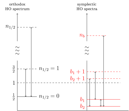
Figure 3: Comparison of the orthodox and the symplectic spectra of the HO, with indications of possible transitions between levels (ignoring any selection rules)

If $\omega_{2}\neq\omega_{1}$ (occurs for diatomic molecules with different isotopic atoms and for electronic transitions between local minima of different Born-Oppenheimer potentials for the nuclei; see below), one has

$$(E_{b_{1},n_{b_{1}}^{\prime}}-E_{b_{2},n_{b_{2}}^{\prime\prime}})/\hbar=\omega_{1}[n_{b_{1}}^{\prime}-\sigma\,n_{b_{1}}^{\prime\prime}+b_{1}-\sigma b_{2}],~{}\sigma=\frac{\omega_{2}}{\omega_{1}}.$$ (218)

4. As discussed in Section III.B above, for a given $\omega$ one needs the time $t_{s},\,\omega\,t_{s}=2\pi s\,,\,s\in\mathbb{Z},$ in order to “run” through an $s$-fold covering $\mathbb{S}^{1}_{[s]}$ of the circle $\mathbb{S}^{1}$. The prefactor $\exp(-ib\,\omega t)$ of the general state (92) shows that here the time “angle” $\tilde{t}=\omega t$ can be reduced by a small $b\ll 1/2$!

For infrared light the number $s$ of coverings is obviously very large for a finite time interval $\Delta t\gg T=1/(2\pi\omega)$, where $\omega\approx 10^{14}$Hz in the near infrared.

5. In Section III.D above we discussed the $n\to n\pm 1$ transition amplitudes for the “primitive” effective Hamiltonian (107) the interaction term of which mimics partial properties of an electric dipole moment. If one wants to include the influence of external electromagnetic radiation, one has to allow the coupling term $g$ to depend explicitly on time or via other external parameters or fields Merzbacher (1970).

6. For experimental tests it is essential to find quantities (“observables”) which are especially sensitive to values of the B(argmann)-index $b$. The following is an - incomplete - list of possible theoretically interesting experiments (without proper knowledge of their feasibility in the laboratory or of their observability in the sky)!

IV.2 Vibrating diatomic molecules

Among the most important and interesting oscillators the above results may apply to are vibrating diatomic molecules (for introductions to their physics see, e.g. the textbooks Herzberg (1950); Landau and Lifshitz (1965); Gasiorowicz (1974); Atkins et al. (2018); Atkins and Friedman (2005); Parigger and Hornkohl (2020)). They have one vibrational degree of freedom: oscillations about the point of equilibrium along the line connecting the two nuclei (“internuclear axis” = INA). Near that equilibrium point the potential may be considered to be harmonic. In the Born-Oppenheimer (BO) approximation the effective potentials for the vibrating nuclei are provided by energy configurations of the electron “cloud” the dynamics of which depends only “adiabatically” on the state of the nuclei, especially on their distance $R$ (see Fig.4).

The (classical) angular frequency $\omega=2\pi\nu$ for the mutual harmonic vibrations of the nuclei is given by

$$\omega=2\pi\,\nu=\sqrt{k/\mu},$$ (219)

where $k$ is the “force constant”, determined - in the BO approximation - solely by the actual electronic configuration and $\mu=m_{1}\,m_{2}/(m_{1}+m_{2})$ is the “reduced” mass of the two vibrating atoms.

Spectroscopists denote the vibrational level numbers $n$ of the HO by $v$ and give the frequencies $\nu\,$[s^-1] in terms of the “wave number” $\tilde{\nu}=\nu/c\,$[cm^-1]. One then has the (approximate) equivalences

$$1\,\text{eV}\cong 8066\,\text{cm}^{-1}\cong 11605^{\circ}\text{ K}.$$ (220)

Spectroscopically the differences between homonuclear (equal nuclei like molecular hydrogen H₂ or oxygen O₂) and heteronuclear (different nuclei like carbon monoxyde ¹²C¹⁶O) diatomic molecules are important: because of space reflection symmetry the homonuclear molecules do not have a permanent electric dipole moment and, therefore, no corresponding infrared emissions or absorptions lan . If, however, their polarizability is nonvanishing, they can have induced electric dipole moments, e.g. in case of elastic and inelastic Raman-type scattering or by collisions.

In addition to the vibrational energy levels characterized by the numbers $v=0,1,2\ldots$ the diatomic molecules have rotational levels $J=0.1.2,\ldots$ due to the rotations of the molecule around an axis which lies in a plane perpendicular to the INA and passing through the centre of mass on that axis. So in general one has the combined vibration - rotation (“rovibrational”) transitions $(v^{\prime},J^{\prime})\to(v^{\prime\prime},J^{\prime\prime})$. The frequencies of the vibrational transitions are generally in the “near-infrared” (frequencies around $\nu\approx 10^{14}$ s^-1) and those of the rotational ones are at least one order of magnitude smaller and are in the “far-infrared” or microwave region.

Example: Molecular hydrogen H₂

Here are some essential properties of the molecule H₂ which are importent for our present discussion: As a homonuclear diatomic molecule H₂ has no permanent electric dipole moment (this property is frequently mentioned in the literature, but very rarely proven; for a proof see Ref. lan ). Because of this missing electric dipole moment their is no corresponding infrared emission or absorption.

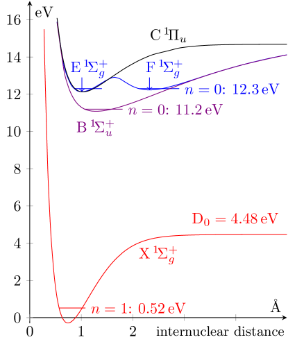
Figure 4: Some of the lowest ”binding” electronic BO potentials for the vibrations of the two H₂ nuclei as a function of their distance $R$. The zero energy on the ordinate coincides with the zero-point energy of the electronic potential X ${}^{1}\Sigma^{+}_{g}$. The numerical values are taken from Ref. Sharp (1971). For the interpretation of the terms denoting the different curves see Appendix B.

There is, however, (weak) magnetic dipole and electric quadrupole infrared radiation et al. (2019a).

Due to that missing electric dipole moment there are no direct vibrational transitions $v\leftrightarrow v\pm 1$ within a given electronic BO – potential, like the electronic ground state potential X ${}^{1}\Sigma^{+}_{g}$ (see Fig. 4).

As a consequence, in order to experimentally analyse the ladder of vibrational states of, e.g. the BO electronic ground state potential X ${}^{1}\Sigma^{+}_{g}$, an “ultraviolet detour” has to be taken: one first initiates an ultraviolet allowed (1- or 2-$\gamma$) absorptive transition from the electronic ground state to a vibrational level of a higher BO electronic potential (Fig. 4), from where the photons cascade down (in 1 or more steps) to a vibrational level of X ${}^{1}\Sigma^{+}_{g}$ which is different of the one the photons originally started from. The difference of the observed ultraviolet frequencies then provides information about the vibrational levels of the selected BO potential Sharp (1971); Glass-Maujean et al. (1984); Sternberg (1989); et al. (1993a, b); Roncin and Launay (1994); Bailly et al. (2010); Hancock et al. (2004); et al. (2011, 2013, 2014, 2018b).

The “ultraviolet detour” also plays an essential role in the so-called “Solomon process” which leads to photodissociation of H₂ Field et al. (1966); Stecher and Williams (1967); loe (a); Loeb and Furlanetto (2013).

Another possibility to observe vibrational and rovibrational levels of H₂ electronic BO potentials is provided by the polarizability of the molecule, which allows for Raman-type transitions associated with induced electric dipole moments, induced by by external light beams or be collisionspol (a); Veirs and Rosenblatt (1987); McCann and Hampton (1994); Long (2002); Li and et al. (2018).

The two nuclei (protons) oscillating in the binding electronic BO potentials may have antiparallel spins (para-H₂) or parallel ones (ortho-H₂). For recent summeries and reviews of the role of H₂ in different areas of physics see, e.g. Field et al. (1966); Sharp (1971); Sprecher et al. (2011); Ubachs et al. (2016); et al. (2017, 2019b). More references will be quoted in the course of the discussions below. (Numerical values of quantities mentined below are rounded up/down from their impressively determined accurate theoretical and experimental values).

For the nuclear vibrations of the diatomic homonuclear molecules H₂ in the electronic ground state X ${}^{1}\Sigma^{+}_{g}$ BO potential (Fig. 4) one has for the “transition” (”ground tone”) et al. (2019c, 2013)

$$(\Delta\,v,\Delta\,J):\, (v^{\prime\prime}=0,J^{\prime\prime}=0)\leftrightarrow(v^{\prime}=1,J^{\prime}=0)$$ (221)

$$\approx(\pm[\tilde{\nu}_{0\leftrightarrow 1}\approx 4161\text{ cm}^{-1}],0)$$

which is one of the larger values for vibrating diatomic molecules.

Recall that the BO electronic ground state X${}^{1}\Sigma^{+}_{g}$ is an effective potential for the vibrations of the two nuclei, depending on their distance $R$ (Fig. 4).

The vibrational transition value (221) correponds to about $0.516\,$ eV, a wave length $\lambda=1/\tilde{\nu}\approx 2,4\,\mu$m and a temperature of $\approx 5988^{\circ}$ K.

In comparison the rotational transition $(0,0)\leftrightarrow(0,1)$ has the wave number $\tilde{\nu}\approx 118$ cm${}^{-1}\cong 0.0146$ eV et al. (2019c). This means a wavelength $\lambda\approx 85\,\mu$m.

If the vibrating H₂ molecule were an ideal HO, its “orthodox” zero-point energy, according to Eq. (221), would be

$$E_{0}(X~{}^{1}\Sigma^{+}_{g}) =\frac{1}{2}\tilde{\nu}_{0\leftrightarrow 1}(X~{}^{1}\Sigma^{+}_{g})$$ (222)

$$\approx 2080\text{ cm}^{-1}\cong 0.258\text{ eV}\cong 2994^{\circ}\text{ K}.$$

The vibrating molecule H₂ is, of course, no ideal HO because it dissociates at a finite energy $D_{0}>E_{0}$. The Morse potential (200) takes this qualitatively into account, as can be seen from the relations (202). The “anharmonic” modifications of energy (204) and angular frequency (205) are small as long as $\omega_{0}I\ll V_{0}$.

The quantum mechanical energy (208) can be written as

$$E_{b,n}=\hbar\omega_{0}\,(n+b)-\frac{(\hbar\omega_{0})^{2}}{4\,V_{o}}(n+b)^{2},$$ (223)

which may be considered as a polynomial in $(n+b)$. As the Morse potential still is only a rough approximation, one has taken - for the orthodox value $b=1/2$ - the expression (223) as a suggestion to parametrize the vibration and rotation levels generally by Dunham (1932); her (a); Irikura (2007)

$$E_{v,J}=\sum_{i\geq 0,j\geq 0}Y_{i,j}\,(v+1/2)^{i}J^{j}(J+1)^{j},$$ (224)

where the coefficients $Y_{i,j}$ are determined (mainly) experimentally. The ground state (“zero-point”) energy is given by

$$E_{0,0}=\sum_{i\geq 0}Y_{i,0}(1/2)^{i}.$$ (225)

For the Morse potential one has $Y_{1,0}=\hbar\omega_{0},\,Y_{2,0}=-\hbar\omega_{0}/(4V_{0})$, all other $Y_{i,0}$ vanishing.

The approximation ansatz (224) gives for H₂ instead of (222) the value Irikura (2007)

$$E_{0}[\text{H}_{2})\approx 2180\text{ cm}^{-1}.$$ (226)

Thus, by passing from the orthodox HO spectrum ($b=1/2$), usually associated with H₂ infrared vibrations, to the symplectic one [$b\in(0,1)$] one can lower the zero-point energy of the BO potential X ${}^{1}\Sigma^{+}_{g}$ maximally by the (approximate) amount

$$E_{0}(H_{2}; b\to 0)-E_{0}(H_{2};b=1/2)\equiv\hat{E}_{0}(H_{2})$$ (227)

$$\approx 2100\text{ cm}^{-1}\cong 0.26\text{ eV}\cong 3000^{\circ}\text{ K }.$$

Similarly, the known dissociation energy of H₂ Sprecher et al. (2011); et al. (2018c, 2019b); Puchalski et al. (2019)

$$D_{0}\approx 36118\text{ cm}^{-1}\cong 4.48\text{ eV}$$ (228)

- theoretically - increases maximally by the the amount (227).

Thus, the orthodox H₂ vibrational spectrum (b = 1/2) can be considerably “detuned” for $1/2>b>0$.

The difference (227) between the orthodox and the symplectic ground states of the vibrating H₂ molecule implies an additional effecive Boltzmann factor

$$e^{-\hat{E}_{0}(H_{2})/(k_{B}T)}=e^{-3000^{\circ}/T}.$$ (229)

Preliminarily ignoring all dynamical mechanisms the last Eq. says that for $T<3000^{\circ}$K the symplectic ground state becomes preferred statistically. This will play a role in our astrophysical discussion below. It also indicates that the symplectic HO spectra may be observed better at very low temperatures.

As mentioned above, in the BO approximation the electronic ground state X ${}^{1}\Sigma^{+}_{g}$ (which includes the action of the nuclear Coulomb potentials on the electrons) provides a potential for the two vibrating nuclei as a function of their distance $R$. The potential has a minimum around which the oscillations are approximately harmonic. The same applies to the next higher electronic (metastable) states B ${}^{1}\Sigma_{u}^{+}$, E F ${}^{1}\Sigma^{+}_{g}$ and C ${}^{1}\Pi_{u}$. They have local minima in appropriate neighbourhoods of which the vibrations are harmonic, too (see Fig. 4).

In the following list one can find the measured energy differences between the ground states of the different electronic levels relative to X ${}^{1}\Sigma^{+}_{g}(v=0,J=0)$ and the energies $E_{0\leftrightarrow 1}$ of the first vibrational excitations $(v=0,J=0)\to(v=1,J=0)$ above those ground states Sharp (1971); Glass-Maujean et al. (1984); Roncin and Launay (1994); et al. (1993a, b, 2006); Bailly et al. (2010); et al. (2011, 2014). The data here are from Ref. Bailly et al. (2010):

$$\geq \text{X}\,^{1}\Sigma^{+}_{g}\,[\text{eV}] E_{0\leftrightarrow 1}\,[\text{eV}]$$ (230)

$$\text{X}\,^{1}\Sigma^{+}_{g}~{}~{}~{}~{}~{} 0 0.52~{}~{}~{}~{}~{}$$

$$\text{B}\,^{1}\Sigma_{u}^{+}~{}~{}~{}~{}~{} 11.19 0.16~{}~{}~{}~{}~{}$$

$$\text{E}\,^{1}\Sigma^{+}_{g}~{}~{}~{}~{}~{} 12.30 0.29~{}~{}~{}~{}~{}$$

$$\text{F}\,^{1}\Sigma^{+}_{g}~{}~{}~{}~{}~{} 12.32 0.15~{}~{}~{}~{}~{}$$

$$\text{C}\,^{1}\Pi_{u}~{}~{}~{}~{}~{} 12.30 0.29~{}~{}~{}~{}~{}$$

The second $E_{0\leftrightarrow 1}$-column shows that the first vibrational excitations are generally quite different for the different electronic levels, reflecting the curvature differences at the minima of the potential curves. If the five BO potentials are approximately harmonic near their minima, the above numerical values of $E_{0\leftrightarrow 1}$ are twice the values of their zero-point energies.

Note that the transitions from (to) the listed higher electronic levels to (from) the electronic ground state X ${}^{1}\Sigma^{+}_{g}(v=0,J=0)$ are in the vacuum UV ($\geq$ 6.20 eV). They are approximately the same as the Lyman $\alpha$ transition of atomic hydrogen (10.20 eV). This is important for a gas mixture of H and H₂: The relative energy differences (230) are all larger than the Lyman $\alpha$ transition and they become even larger for the symplectic spectra. This is important for astrophysical applications (see below).

As mentioned above, in order to determine the vibrational transition energies $E_{0\leftrightarrow 1}$ in the list (230) experimentally one has to take a “detour” of determining related (electronic) UV transitions first and then subtract the corresponding energies Sprecher et al. (2011); et al. (2013, 2018b, 2018c, 2019b).

The set of UV transitions from the states of the potential $\text{X}\,^{1}\Sigma^{+}_{g}$ to those of $\text{B}\,^{1}\Sigma_{u}^{+}$ or vice versa is called the “Lyman-band”, and those of $\text{X}\,^{1}\Sigma_{g}^{+}$ to $\text{C}\,^{1}\Pi_{u}$ the “Werner-band” Glass-Maujean et al. (1984); Roncin and Launay (1994); et al. (1993a, b); Bailly et al. (2010).

IV.3 Vibrations of diatomic molecules
with different isotopic atoms

Such systems played an important but nowadays mostly forgotten role in the early history of quantum mechanics:

Even before Heisenberg derived the now well-established spectrum of the HO in his famous paper from July 1925 Heisenberg (1925), Mullikan had concluded from his investigations of diatomic molecules that their vibrational spectra should be described by half-integers, not integers as the Bohr-Sommerfeld quantization prescription had suggested M. Born, unter Mitwirkung von F. Hund (1925); bor . Mullikan compared the vibrational spectra of diatomic molecules in which one atom was replaced by an isotope (B¹⁰O and B¹¹O; AgCl³⁵ and AgCl³⁷) Mullikan (1925).

Classically the vibrating atoms have angular frequences $\omega_{i}=\sqrt{k/\mu_{i}}$,  where the $\mu_{i},i=1,2$ denote the reduced masses of the oscillators, $\mu_{1}$ for one and $\mu_{2}$ for the other molecule containing one or two isotopic atoms. The (electronic) oscillator strength $k$ is assumed to be the same in both cases (BO approximation).

Let $E_{0}(i)=\gamma\,\hbar\omega_{i}$ be the two slightly different oscillator ground state energy levels for the two “isotopic” oscillators. Let further $E_{a}$ and $E_{b}$ be two known electronic energy levels (they may be equal) from which transitions to the ground states with energies $E_{0}(i)$ are possible. Then the difference

$$\omega_{a,1}-\omega_{b,2}=(E_{a}-E_{b})/\hbar-\gamma(\omega_{1}-\omega_{2})$$ (231)

of the frequencies

$$\omega_{a,1}=[E_{a}-E_{0}(1)]/\hbar,\;\;\omega_{b,2}=[E_{b}-E_{0}(2)]/\hbar$$ (232)

can be used in order to determine $\gamma$. Mullikan concluded that $\gamma\approx 1/2$. A good review of the method can be found in Ref. her (c).

Due to the tremendous experimental and technological advances since those experiments from almost 100 years ago it appears possible to perform similar more refined experiments et al. (2013) in order to find fractional values of the B-index $b$ other than $1/2$. However, one first has to account for the deficits of the BO approximation and for the corrections due to rotational, electronic and QED effects Pachucki (2010); Puchalski et al. (2019)!

IV.4 Interferences of time dependent energy eigenstates

Applying the unitary time evolution operator (75) to the energy eigenstates $|b,n\rangle$ yields ($\hbar=1$ in the following)

$$U(\tilde{t})\,|n,b\rangle=e^{-i(n+b)\tilde{t}}|n,b\rangle,\;\tilde{t}=\omega\,t.$$ (233)

Reccall that $\tilde{t}$ is a (dimensionless) angle variable. Let $\tilde{t}$ increase by an amount $\delta\,\tilde{t}$ which may be implemented by either a change of $\omega$ or of $t$ or of both. Consider the superposition

$$|n,b;\tilde{t},\delta\tilde{t}\rangle=(1+e^{-i(n+b)\delta\tilde{t}})e^{-i(n+b)\tilde{t}}|n,b\rangle.$$ (234)

Then the oscillations of the “intensity”

$$|\langle n,b;\tilde{t},\delta\tilde{t}|n,b;\tilde{t},\delta\tilde{t}\rangle|^{2}=4\cos^{2}[(n+b)\delta\tilde{t}/2].$$ (235)

are sensitive to the value of $b\delta\tilde{t}$, especially for $n=0$. For an analogous approach in a recent experiment see Ref. et al. (2019d).

An alternative to generate such interferences by a change $\delta\tilde{t}$ one may also use - at least theoretically - a change $\delta b$. The question, how to generate states like $|n,b\rangle$ experimentally has, unfortunately, to be left open here.

IV.5 Transitions associated with the Hamiltonian $H(K)=\hbar\,\omega\,\tilde{C}_{g}(K)$

In case the model Hamiltonian (107) with its ”effective” electric dipole moment can somehow be implemented experimentally, either by heteronuclear molecules like. e.g. ⁷LiH (it has the rather large electric dipole moment 5.9 D[ebeye]) or by Raman-type induced electric dipole moments of homonuclear diatomic molecules, then especially the transitions (111) depend sensitively on the value of $b$: The probability for the transition $n=0\leftrightarrow n=1$ is given by

$$|\langle b,m=0|\tilde{C}_{g}(K)|b,n=1\rangle|^{2}=b\,g^{2}/2.$$ (236)

So, if the index $b$ is very small $>0$ - as it appears to be in astrophysical cases (see below) - then the same holds for that transition probability!

Another essential point here is that the spectrum $\{n+b\}$ of $\tilde{K}_{0}$ is rescaled for $\tilde{C}_{g}(K)$ by an overall ”redshifting” factor $\sqrt{1-g^{2}}$ (see Eq. (197)).

IV.6 Traps for neutral molecules and optomechanics

A speculatively optimal experimental situation would be a diatomic neutral molecule in a cooled down trap which allows the vibrational emission and absorption properties of the molecule to be observed, especially those of its different electronic potential ground states. As already stressed above, the conditions are different for heteronuclear and homonuclear molecules, the former having an electric dipole moment, the latter not, which requires some Raman-type excitations. In view of the very impressive developments of experimental possibilities involving such traps Grimm et al. (2000); Leibfried et al. (2003); Ashkin (2006), it appears possible to achieve at least a few of the required aims. Closely related are optical devices coupled to mechanical oscillators Aspelmeyer et al. (2014); et al. (2019d, 2020c); Qiu et al. (2020)

IV.7 Perelomov coherent states

Among the three different types of coherent states kas (i) associated with the Lie algebra (52), the so-called “Perelomov” coherent states appear to be the most promising ones in order to detect traces of HO spectra with $b\neq 1/2$: Their matrix elements contain the Bargmann index $b$ quite explicitly and they can be generated experimentally kas (i).

The states $|b,\lambda\rangle$ can either be defined as eigenstates of a composite “annihilation” operator,

$$E_{b,-}|b,\lambda\rangle= \lambda\,|b,\lambda\rangle,\;\;E_{b,-}=(\tilde{K}_{0}+b)^{-1}\tilde{K}_{-},$$ (237)

$$\lambda=|\lambda|e^{-i\theta}\in\mathbb{D}=\{\lambda\in\mathbb{C},\;|\lambda|<1\},$$

or by generating them from the ground state $|b,0\rangle$ by means of the unitary operator

$$U(\lambda)_{P}= e^{(w/2)\tilde{K}_{+}-(w^{\ast}/2)\tilde{K}_{-}}=e^{\lambda\,\tilde{K}_{+}}e^{\ln(1-|\lambda|^{2})\tilde{K}_{0}}e^{-\lambda^{\ast}\tilde{K}_{-}},$$ (238)

$$w=|w|e^{-i\theta}\in\mathbb{C},\;\;\lambda=\tanh(|w|/2)e^{-i\theta},$$

$$|w|=\ln\left(\frac{1+|\lambda|}{1-|\lambda|}\right),$$

so that

$$|b,\lambda\rangle=U(\lambda)_{P}|b,0\rangle.$$ (239)

In terms of number states we have the expansion

$$|b,\lambda\rangle =(1-|\lambda|^{2})^{b}\sum_{0}^{\infty}\left(\frac{(2b)_{n}}{n!}\right)^{1/2}\lambda^{n}|b,n\rangle,$$ (240)

$$(2b)_{n} =2b(2b+1)\ldots(2b+n-1)=\Gamma(2b+n)/\Gamma(2b),$$

$$~{}~{}~{}~{}(2b)_{n=0}=1.$$

Note that the coefficient of $\lambda^{n}$ in this expansion is the same as that of $e_{n}(\vartheta)$ in Eq. (140).

Important expectation values with respect to $|b,\lambda\rangle$ are

$$\langle b,\lambda|\tilde{K}_{0}|b,\lambda\rangle\equiv \overline{\tilde{K}_{0}}_{;b,\lambda}=b\cosh|w|,$$ (241)

$$\langle b,\lambda|\tilde{K}_{1}|b,\lambda\rangle\equiv \overline{\tilde{K}_{1}}_{;b,\lambda}=b\sinh|w|\,\cos\theta,,$$ (242)

$$\langle b,\lambda|\tilde{K}_{2}|b,\lambda\rangle\equiv \overline{\tilde{K}_{2}}_{;b,\lambda}=-b\sinh|w|\,\sin\theta,$$ (243)

$$\langle b,\lambda|N|b,\lambda\rangle\equiv \overline{N}_{b,\lambda}=b(\cosh|w|-1),$$ (244)

$$(\Delta N)^{2}_{b,\lambda}\equiv \overline{N^{2}}_{b,\lambda}-\overline{N}_{b,\lambda}^{2}=\frac{1}{2}b\sinh^{2}|w|$$ (245)

It follows that most quantities can be expressed in terms of the “observables” $\overline{N}_{b,\lambda}$ and $(\Delta N)_{b,\lambda}$: As

$$b\sinh|w|=\sqrt{2b}(\Delta N)_{b,\lambda}$$ (246)

and $\cosh|w|=(\sinh^{2}|w|+1)^{1/2}$ we have, e.g.,

$$\overline{\tilde{K}_{0}}_{;b,\lambda}= [2b(\Delta)^{2}_{b,\lambda}+b^{2}]^{1/2},$$ (247)

$$\overline{N}_{b,\lambda}[1+\overline{N}_{b,\lambda}/(2b)]= (\Delta N)^{2}_{b,\lambda}.$$ (248)

It follows from the last equation that Paul’s parameter R Paul (1999) here has the value

$$R_{b,\lambda}\equiv\frac{(\Delta N)^{2}_{b,\lambda}-\overline{N}_{b,\lambda}}{\overline{N}_{b,\lambda}^{2}}=\frac{1}{2b}.$$ (249)

$R$ is a measure for deviations from a Poisson distribution for which $(\Delta n)^{2}-\bar{n}=0$.

In addition we have

$$|\lambda|= \tanh(|w|/2)=\frac{\cosh|w|-1}{\sinh|w|}=\frac{\overline{N}_{b,\lambda}}{\sqrt{2b}(\Delta N)_{b,\lambda}}$$ (250)

$$|\lambda|^{2}= \frac{\cosh|w|-1}{\cosh|w|+1}=\frac{\overline{N}_{b,\lambda}}{\overline{N}_{b,\lambda}+2b}$$ (251)

and

$$|w|=\ln\left(\frac{1+|\lambda|}{1-|\lambda|}\right)=\ln\left[\frac{1+(1+2b/\overline{N}_{b,\lambda})^{1/2}}{(1+2b/\overline{N}_{b,\lambda})^{1/2}-1}\right].$$ (252)

For $\overline{N}_{b,\lambda}/2b\gg 1$ the last relation reduces to

$$|w|\approx\ln(2\overline{N}_{b,\lambda}/b).$$ (253)

The transition probability

$$p_{b}(n\leftrightarrow\lambda)=|\langle b,n|b,\lambda\rangle|^{2}=(1-|\lambda|^{2})^{2b}\frac{(2b)_{n}}{n!}|\lambda|^{2n}$$ (254)

can be expressed as (see Eq. (251))

$$p_{b}(n\leftrightarrow\lambda)= \frac{(2b)_{n}(2b)^{2b}\overline{N}_{b,\lambda}^{n}}{n!\,(\overline{N}_{b,\lambda}+2b)^{n+2b}},$$ (255)

$$p_{b}(0\leftrightarrow\lambda)= \frac{(2b)^{2b}}{(\overline{N}_{b,\lambda}+2b)^{2b}}.$$ (256)

Comparing the classical quantities (14) with the relations (73) and (241) - (243) one infers the classical limit

$$I\asymp\lim_{(\hbar b)\to 0,|w|\to\infty}[(\hbar b)\cosh|w|\asymp(\hbar b)\sinh|w|]$$ (257)

IV.8 (Dispersive) van der Waals forces

F. London was the first one to associate the attractive van der Waals forces between neutral atoms or molecules with the nonvanishing zero-point energy of the HO Eisenschitz and London (1930); London (1930, 1931, 1937). For atoms or molecules of the same type and without retardation he derived - using a HO model - the potential (see also Refs. mil ; Milonni (1994))

$$V(R)=-\gamma(\frac{1}{2}\hbar\omega)\,\frac{\alpha^{2}}{R^{6}},$$ (258)

where $\gamma>0$ is a number of order 1, $\alpha$ the (static) polarizability of the two atoms or molecules pol (a); atk , $R\leq\lambda=(2\pi c)/\omega$ the distance of their nuclei and $\omega$ the angular frequency of an oscillating electric field mode which acts, e.g., either on the permanent electric dipole moments of two molecules or on the their induced electric dipole moments. If $\vec{d}$ is the electric dipole moment generated at its position by the effective electric field $\vec{E}_{\mathit{eff}}$, then $\alpha$ in an isotropic situation is defined by $\vec{d}=\alpha\,\vec{E}_{\mathit{eff}}$. It has the dimension $[L^{3}]$ ($\vec{E}_{\mathit{eff}}$ includes a charge factor). The relation (258) holds for vanishing temperature $T$ (for $T>0$ see, e.g. Ref. Passante and Spagnolo (2007)). It is proportional to the usual HO ground state energy $\hbar\omega/2$.

The potential (258) is of special importance for atoms and molecules which do not have a permanent electric dipole but an induced one like, e.g. atomic hydrogen H or molecular hydrogen H₂, both in their ground states. The corresponding values are

$$\alpha[H(^{1}S)]=0.67\cdot 10^{-30}m^{3},~{}~{}~{}\alpha[H_{2}(^{1}\Sigma_{g}^{+})]=0.79\cdot 10^{-30}m^{3}$$ (259)

pol (b). As the polarizability $\alpha$ is closely related to the dispersion properties of an optical medium Born and Wolf (1999), London called the forces associated with the potential (258) “dispersion” van der Waals forces London (1937).

If one applies London’s London (1930, 1931, 1937) and later heuristic arguments Kleppner ; mil for the derivation of the van der Waals potential to the symplectic spectrum of the HO, one obtains instead of Eq. (258):

$$V(R)=-\gamma(b\,\hbar\omega)\,\frac{\alpha^{2}}{R^{6}}.$$ (260)

If $b<1/2$ the “symplectic” van der Waals forces are weaker than the “orthodox” ones.

The closely related Casimir effect Casimir and Polder (1948); Casimir (1948); Schwinger (1975); Schwinger et al. (1978); Plunien et al. (1986); Milonni (1994); Mostepanenko et al. (1997); Milton (2001); et al. (2004); Genet et al. (2004); Milton (2004); Jaffe (2005); Kawakami et al. (2007); Lamoreaux ; Reynaud and Lambrecht (2017) has to be discussed separately, due to its different derivations and interpretations!

V Possible astrophysical implications

In case the above theoretically possible “symplectic” - or “fractional” - spectra (69) of the HO are - at least partially - realized in nature they could shed new light on some unsolved basic astrophysical problems of which I shall mention the two most important ones et al. (b):

Dark energy et al. (Particle Data Group); Olive and Peacock ; Weinberg and White ; Frieman et al. (2008) and dark matter Bertone and Hooper (2018); Baudis and Profumo . Here the symplectic spectra (69) may be a (the) key to the solutions of both problems simultaneously!

For reasons mentioned above those spectra have not yet been seen in the laboratory. But, surprisingly, physical implications of those spectra are supported by the observationally favoured cosmological $\Lambda$CDM model Peebles (1993); Ellis (2018); Turner (2018); Olive and Peacock ; Collaboration (a) and by the associated WIMP hypothesis Feng (2010); Bertone and Hooper (2018); et al. (2018d); Schumann (2019).

It probably sounds provocative, but the observed dark energy and dark matter properties may provide the first empirical support for the existence of the spectra (69) in nature!

The following discussions and arguments are mostly qualitative. The obviously necessary and crucial quantitative arguments will still have to be reviewed and worked out in detail!

V.1 Dark energy and the cosmological constant

Describing the existing astrophysical observations in terms of the Einstein-Friedmann-Lemaître cosmological model Olive and Peacock ; Lahav and Liddle leads to the conclusion that the (“vacuum”) energy density $c^{2}\rho_{\Lambda}$, associated with the so-called “Lambda”-term in the Einstein-Friedmann-Lemaître equations, has the same order of magnitude as the critical energy density lam

$$c^{2}\rho_{crit}=3c^{2}H_{0}^{2}/(8\pi G_{N})\approx 10^{-5}h^{2}\,\text{GeV}\,\text{cm}^{-3},$$ (261)

where the scale factor $h$ for the present Hubble expansion rate $H_{0}$ has the approximate value $h\approx 0.7$ (this “astrophysical” $h$ is not to be confused with Planck’s constant in the following):

Taking into account that the observed “dark” energy density $c^{2}\rho_{\Lambda}$ is about $0.7$ of the critical density (261) Weinberg and White and equating $c^{2}\rho_{\Lambda}$ with the vacuum energy density of the quantized free electromagnetic field kas (j),

$$u_{em;0}(\hat{\omega},b)=\frac{b\,\hbar}{4\pi^{2}\,c^{3}}\,\hat{\omega}^{4},$$ (262)

where $\hat{\omega}$ is an appropriate cutoff for the corresponding divergent frequency integral

$$u_{em;0}(b)=\frac{b\,\hbar}{\pi^{2}\,c^{3}}\,\int_{\omega\geq 0}d\omega\,\omega^{3},$$ (263)

allows to make a numerical estimate of $b$:

Introducing the cutoff length

$$\ell=\frac{2\pi c}{\hat{\omega}}$$ (264)

leads to the approximate equality

$$u_{em;0}(\ell,b)=b\frac{4\pi^{2}\,\hbar c}{\ell^{4}}\,\approx 0.7\cdot c^{2}\rho_{crit}.$$ (265)

Taking for $\ell$ the (reduced) Compton wave length of the electron,

$$\ell\approx\lambdabar=\hbar/(m_{e}c)\approx 3.9\cdot 10^{-11}\text{cm}$$ (266)

and inserting $h^{2}\approx 0.5$ into relation (261) gives for the B-index $b$ the approximate value

$$b\approx 10^{-35}\,.$$ (267)

This is an extremely small $b$ – value, but it is theoretically allowed in the present framework! This is in contrast to the conventional theoretical estimates of the dark energy with $b=1/2$ Weinberg (1989); Carroll et al. (1992); Carroll (2001); Frieman et al. (2008) which represent the most embarrassing discrepancy between observations and theoretical reasoning in all of present-day physics!

The discussion above assumes that all modes have the same index $b$. This simplification is, of course, not necessary. $b$ can depend on the frequency $\omega$: $b=b(\omega)\in(0,1]$. It can, therefore, become a dynamical quantity!

The estimate (267) depends sensitively on the choice of the cutoff length $\ell$: if we. e.g., replace the factor $10^{-11}$ by $10^{-10}$ the estimate in Eq. (267) is reduced to $b\approx 10^{-31}$. In addition all non-electromagnetic effects were neglected (they would lead to an even smaller value of $b$ than that in Eq. (267)!). This will be justified by the discussion below concerning the nature of dark matter as being essentially molecular hydrogen the dynamics of which is essentially determined by electromagnetic forces.

Let me make another very crude estimate related to the “cosmic” order of magnitude (267) of the B-index $b$: Consider the relation (84) between the angular frequency $\omega=2\pi\nu$, the time period $T_{2\pi;b}$ and the index $b$: Most of the very first molecules and molecular ions after the beginning of the recombination epoch in the very early universe were diatomic, with the vibrating nuclei locally emitting infrared light with frequencies $\nu=\omega/(2\pi)$ around $10^{14}~{}$s^-1. Even though homonuclear elements like $H_{2}$ do not have a permanent electric dipole element, they still radiate in the infrared et al. (2019a) and especially can emit Raman radiation by induced dipole momennts (see Ch. IV.B above).

Taking for $T_{2\pi;b}$ the extreme value $10^{10}$ yr $\approx 3\,\cdot 10^{17}$ s and ignoring cosmic red shifts $z$ (i.e. being in the rest frame of the molecule) we get the crude estimate

$$b=1/(\nu\,T_{2\pi;b})\approx 10^{-32}.$$ (268)

An important open question is whether the vacuum (“dark”) energy has changed with cosmic time which would imply a corresponding time dependence of $b\,$!

V.2 “Dark” b-H₂ and other primordial molecules
as dark matter?

The following most intriguing but perhaps also dangerously seductive or even deceptive attempt intends to interpret the cosmic “dark matter” in the “symplectic” framework of the HO. The central hypothetical role here is being played by “symplectic” molecular hydrogen b-H₂ as the main candidate for dark matter. The possibility that molecular hydrogen H₂ may play a role for the understanding of dark matter has been tentatively discussed before Carr (1994); Pfenniger et al. (1994); Pfenniger and Combes (1994); Combes and Pfenniger (1997); Combes and des Forêts (2000); Combes ; Paolis et al. (1995a, b); et al. (1995); Paolis et al. (1999); Gerhard and Silk (1996) without, it seems, having a lasting impact. But the possible existence of a (weak or hidden) “detuned” symplectic spectrum of the vibrating b-H₂ allows for a new and probably more promising approach! In addition to this ”symplectic” detuning there is, of course, the usual cosmic redshift $z$ due to the expansion of the universe.

All the directly obtained experimental and obervational data like those of the “Planck” Kollaboration etc. are, of course, not affected, but all the calculated particle and cosmic standard model dependent dynamical - vibration related - electromagnetic properties (transition probabilities of emissions, absorptions, dissociations, ionizations and other rates etc.) have to be re-evaluated. The same applies to the Big Bang Nucleosynthesis and the primordial photon-baryon ratio Cybert et al. (2016); Fields et al. !

Molecular hydrogen plays already an important role in the present standard (“orthodox”) cosmological paradigm Field et al. (1966); Peebles (1993); Williams (1999); Combes and des Forêts (2000); Galli and Palla (1998); Lepp et al. (2002); Snow and McCall (2006); Galli and Palla (2013); Loeb and Furlanetto (2013); Ubachs et al. (2016); et al. (2017). Due to the missing electric dipole moment it is difficult to detect astrophysically. For searches in the intergalactic medium (IGM) one uses a plausible correlation between the densities of H₂ and of carbon monoxyde CO Bolatto et al. (2013), which has a permanent electric dipole moment and is more visible. But the atoms C and O are not primordial ones and have to be bred in (first) stars etc..

Presently, however, we are primarily interested in the epoch of the universe which is called its “Dark Ages” Barkana and Loeb (2001); Miralda-Escudé (2003); Loeb ; loe (b); et al. (a), i.e. the cosmic time period which started when the photons decoupled from matter and primordial atoms (mainly He and H) could form (“recombination epoch” pee ; Peacock (1999); pea ; Barkana and Loeb (2001); Mukhanov (2005); muk ; Weinberg (2008); wei ) at about 400000 years after the big bang (at redshift $z=z_{\star}\approx 1100\approx 3000^{\circ}$ K$\approx 0.26$ eV Collaboration (b)). And which ended just before (around $z\approx 30$, i.e. about 80 Myr after the big bang) density fluctuations of the primordial gases led to the first gravitational “clumps” as seeds for the first stars Barkana and Loeb (2001); Naoz et al. (2006); Loeb and Furlanetto (2013); Fialkov et al. (2012) and the first galaxies Bromm and Yoshida (2011); Loeb and Furlanetto (2013). The heat and radiation associated whith this gravitational process reionized the primordial neutral gases of the dark ages Fan et al. (2006); Loeb and Furlanetto (2013), a cosmic period called the “Dawn” of the universe et al. (a).

During those “dark ages” there were no “dust grains”, no “metals” (like ¹⁶O or ¹²C etc.) and no X- and no cosmic rays. There were only gases of primordial photons, neutrinos, electrons, protons, deuterons and atoms He, H, D, Li, their ions and first primordial diatomic molecules and their ions Galli and Palla (1998); Lepp et al. (2002); Galli and Palla (2013) like H₂ and, e.g. (HeH)⁺ Dabrowski and Herzberg (1977); Zygelman et al. (1998); Bovino et al. (2011); Galli and Palla (2013); et al. (2019e) most of them at least partially in local thermodynamical equilibrium. Ions may be “thrown” out of equilibrium by primordial magnetic fields.

As the main observable signal from that epoch the 21 cm line from the electron spin flip in the field of the magnetic moment of the proton in atomic hydrogen has intensively been discussed more recently Barkana and Loeb (2001); Furlanetto et al. (2006); Pritchard and Loeb (2012); Barkana (2016); Cohen et al. (2017, a); Novosyadlyj et al. (2020); et al. (a) and experimentally implemented or planned Monsalve et al. (2017); et al. (2018a, a). Molecular hydrogen is also assumed to play an essential role during the dark ages Barkana and Loeb (2001); Hirata and Padmanabhan (2006); Alizadeh and Hirata (2011); Novosyadlyj et al. because of its cooling properties Loeb and Furlanetto (2013); Barkana (2016).

In the following a number of possibly important properties of “symplectic” molecular hydrogen, called b-H₂, are listed which support the hypothesis of essentially identifying dark matter with b-H₂. The $b$-detuned spectra of other primordial diatomic molecules (containing D, He and Li Galli and Palla (1998); Lepp et al. (2002); Galli and Palla (2013)) probably play an essential role, too, but that of b-H₂ is the most important one and here serves as a prototype for a symplectically detuned molecular HO! The following discussion relies on properties of b-H₂ pointed out in Ch. IV.B above.

What is still missing in the discussion presented here is a necessary critical quantitative evaluation! This is, of course, due to the fact that up to now no corresponding experimental laboratory data are available and - above all - that the associated theory for the dynamics of the “symplectic” spectroscopy still has to be worked out! But in principle it should be possible to decide the empirical existence of those symplectic spectra in the laboratory, keeping in mind that the index $b$ might be very small (see Eq. (267)) and, therefore, optical transitions may be very weak (slow)!

Here is a list of properties and problems which shows how the b-H₂ (plus other primordial molecules) dark matter hypothesis compares with what essentially is known about dark matter experimentally:

1. It is quite surprising that the measured (relative) cosmic baryonic density $\Omega_{b}\approx 0.05$ and the dark matter density $\Omega_{d}\approx 0.25$ are roughly of the same order of magnitude. And that the total matter density $\Omega_{m}\approx 0.3$ is about of the same order of magnitude as the dark (“vacuum”) energy density $\Omega_{\Lambda}\approx 0.7$! But this is no longer surprising if dark matter consists essentially of “b-”H₂ and other “b”-detuned primordial molecules, i.e. it is baryonic, too ! In addition there may be some kind of dynamical relationships between vacuum energy and matter.

2. Whereas there appears to be - on average - 5 times more dark than baryonic matter in the universe, not a single non-standard particle has been detected, despite years-long tremendous and ingenious efforts by experimentalists and theoreticians Feng (2010); Bertone and Hooper (2018); Baudis (2012); et al. (2018d); Salucci (2019); Schumann (2019). That failure is no surprise if dark matter essentially consists of b-H₂ and other b-detuned primordial diatomic molecules and ions!

3. If indeed dark matter consists of such molecules and ions, this implies that there is no dark matter in the universe before the recombination/decoupling era when the formation of primordial atoms (He, H, D, Li), their molecules and ions sets in Galli and Palla (1998); Lepp et al. (2002); Loeb and Furlanetto (2013); Galli and Palla (2013). And there is then no annihilation of dark matter!

4. For the formation of b-H₂ etc. as dark matter about 5 times more primordial baryons and electrons are required. This needs, of course, a re-evaluation of the orthodox big bang nucleosynthesis (BBN) and the related baryon to photon ratio Peacock (1999); Mukhanov (2005); Weinberg (2008); Cybert et al. (2016); Fields et al. ; Olive and Peacock .

5. The dark matter approach discussed here may also shed some new light on the “Lithium problem” of the current BBN interpretation (a disturbing discrepancy between the observed Li/H ratio und the BBN predicted one) lit .

6. If there are at the beginning of the recombination phase - ignoring all other light primordial nuclei, their atoms, molecules and ions - protons and electrons, why should they form dominantly b-H₂ molecules and H atoms so that on average we have a ratio of approximately 5:1? A preliminary argument is that the b-H₂ molecules are energetically favoured compared to 2 free H atoms because of their binding energies (4.48 + 0.26 = 4,74) eV (see Eqs. (228) and (227)). In order to understand the observed ratio 5:1 of “dark” matter to baryonic matter one probably has to take the dynamics of the different atomic and molecular reactions into account! Note that the formation of primordial hydrogen molecules can take different routes Galli and Palla (1998); Lepp et al. (2002); Galli and Palla (2013).

7. It also is worth mentioning that the “partial” Boltzmann factor (229) becomes smaller than of order 1 just at the beginning of the dark ages. This implies that as lower temperatures statistically the lower b-zero-point energy levels are correspondingly more populated than the “orthodox” ones!

8. Even if the transitions between the detuned b-levels of the vibrating molecules are very weak there should be enough time (60-100 Myr) available during the dark ages to “settle down” to the b-zero-point energy levels.

9. Galaxies (first small ones which then became larger) are assumed to have grown from (Jeans) density perturbations/fluctuations leading to instabilities inside halos of dark matter Loeb and Furlanetto (2013); Wechsler and Tinker (2018); Salucci (2019); et al. (2020d); Inayoshi et al. (2020). That appears quite “natural” if those halos are essentially cold remains of primordial diatomic molecular (mainly hydrogen) clouds from the dark ages, in which most of the molecules are not yet dissociated. Consequently one has to expect dynamical relations between the ionized core of galaxies (including their stars, black holes and gases) and their dark cold molecular halos.

10. If dark matter consists essentially of b-H₂ and other primordial diatomic molecules and ions then there was a rich amount of matter for the formation of baryonic supermassive black holes in the center of evolving galaxies Bromm and Loeb (2003); Inayoshi et al. (2020).

11. As H₂ is considered to be an important coolant for the primordial gases before the formation of cosmic structures sets in Bourlot et al. (1999); Coppola et al. (2011); Loeb and Furlanetto (2013) the cooling by b-H₂ has to be analyzed anew.

12. Molecular hydrogen has a mass of about 2 GeV. Comparing this with the reconstructed temperature $T_{\gamma}\approx 0.26$ eV of the photon gas at the beginning of the recombination period and assuming the matter gases to have roughly the same temperature about that time implies that the molecules are highly nonrelativistic. The same applies, of course, to the other primordial molecules and ions containing He, D, Li etc.

13. Neutral H₂ molecules interact weakly among themselves and with other neutral atoms or molecules by van der Waals forces McKellar (1990); Flower and Roueff (1998a). In addition, the relation (260) shows that the strength of van der Waals forces becomes weaker than the “orthodox” ones for $b<1/2$. For the interactions of “orthodox” H₂ molecules with atomic hydrogen and helium see, e.g., the Refs. Truhlar and Wyatt (1977); Flower (1997); Flower and Roueff (1998b); Flower et al. (1998).

14. A theoretical analysis of the data obtained by the 21-cm radio wave detector EDGES et al. (2018a) concluded Barkana (2018); Fialkov et al. (2018); Fialkov and Barkana (2019); Cohen et al. (b) that most likely there are interactions beyond the gravitational ones between the primordial atomic hydrogen and the dark matter particles, the latter having a mass of about a few GeV! All this fits - at least qualitatively - the above b-H₂ interpretation of dark matter very well. In addition it supports the hypothesis that dark matter consists of (w)eakly (i)nteracting (m)assive (p)articles (“WIMPs”).

15. The recently observed discrepancy between gravitational lensing et al. (2020a) and computer-simulated (standard) dark matter models may also find an explanation within the framework discussed in the present paper!

16. Of special interest in the context of the near-infrared “symplectic” spectra of H₂ etc. molecules discussed above are the recent unaccounted cosmic optical background observations in that spectral region by the CIBER and New Horizons collaborations Matsuura (2017); et al. (c).

All the properties listed above are - qualitatively - surprisingly compatible with the current $\Lambda$CDM model of the universe and the WIMP hypothesis for dark matter!

All this suggests that the hypothesis: “the dark matter observed in the universe consists essentially of b-H₂ and of a smaller amount of other primordial diatomic b-detuned molecules and their ions” should be taken seriously and analyzed more quantitatively and experimentally as well. This requires joint efforts of the physisists involved in the field!

One particular lesson to be learnt from the discusssions above is that we do not know yet enough about the physics of the cosmic quantum“vacuum”!

Appendix A Hilbert space for $\tilde{K}_{j}$ and $\tilde{C}_{g}(K)$ on $\mathbb{R}_{0}^{+}$

A.1 Representation of the Lie algebra generators $\tilde{K}_{j}$ on $L^{2}(du,\mathbb{R}^{+}_{0})$

The Hilbert spaces of square-integrable functions

$$f(u)=u^{\alpha/2}\,e^{-u/2}g(u),\;u\geq 0,\,\alpha>-1,$$ (269)

with the scalar product

$$(f_{2},f_{1})\equiv \int_{0}^{\infty}du\,f_{2}^{\ast}(u)f_{1}(u)$$ (270)

$$= \int_{0}^{\infty}du\,u^{\alpha}e^{-u}\,g_{2}^{\ast}(u)\,g_{1}(u).$$

also provide Hilbert spaces for irreducible unitary representations of the group $SO^{\uparrow}(1,2)$, its twofold symplectic covering group $Sp(2,\mathbb{R})$ and all other covering groups Boyer and Wolf (1975); ka1 (e).

The usual orthonormal basis for a fixed $\alpha$ is given by the associated Laguerre functions

$$\hat{e}_{\alpha;n}(u)= \sqrt{\frac{n!}{\Gamma(n+\alpha+1)}}\;u^{\alpha/2}\,e^{-u/2}\,L^{\alpha}_{n}(u),\,n=0,1,2,\ldots$$ (271)

$$(\hat{e}_{\alpha;m},\hat{e}_{\alpha;n})=\delta_{mn}\,,$$

where the associated Laguerre polynomials $L^{\alpha}_{n}(u)$ are defined as

$$.L^{\alpha}_{n}(u)= \sum_{m=0}^{m=n}{n+\alpha\choose n-m}\frac{(-u)^{m}}{m!},\;L^{\alpha}_{n}(0)=\frac{(\alpha+1)_{n}}{n!},$$ (272)

$$(a)_{n}=a\,(a+1)\,(a+2)\ldots\,(a+n-1).$$

Examples:

$$L^{\alpha}_{0}(u)=1,~{}~{}L^{\alpha}_{1}(u)=\alpha+1-u.$$ (273)

The polynomials $L^{\alpha}_{n}(u)$ obey the differential equation

$$u\,\frac{d^{2}L^{\alpha}_{n}}{du^{2}}+(\alpha-u+1)\frac{dL^{\alpha}_{n}}{du}+n\,L^{\alpha}_{n}=0.$$ (274)

The operators $\tilde{K}_{j}$ here have the explicit form Bojowald et al. (2000); Kastrup (2007), with $\alpha=2b-1$,

$$\tilde{K}_{0}= -u\,\frac{d^{2}}{du^{2}}\,-\frac{d}{du}+\frac{(2b-1)^{2}}{4u}+\frac{u}{4},$$ (275)

$$\tilde{K}_{1}= -u\,\frac{d^{2}}{du^{2}}\,-\frac{d}{du}+\frac{(2b-1)^{2}}{4u}-\frac{u}{4},$$ (276)

$$\tilde{K}_{2}= \frac{1}{i}(u\,\frac{d}{du}+\frac{1}{2})\,.$$ (277)

They obey the Lie algebra (10). The inequality $\alpha>-1$ (Eq. (269)) implies $b>0$, as desired!

Eigenfunctions $f_{b;n}(u)$ of $\tilde{K}_{0}$ are the basis functions (271) with $\alpha=2b-1$:

$$\tilde{K}_{0}f_{b;n}(u)= (n+b)\,f_{b;n}(u),\,n=0,1,2,\ldots$$ (278)

$$f_{b;n}(u)= \hat{e}_{2b-1;n}(u)$$

$$= \sqrt{\frac{n!}{\Gamma(2b+n)}}\;u^{b-1/2}\,e^{-u/2}\,L^{2b-1}_{n}(u).$$

The ground state function is

$$f_{b;0}(u)=\frac{1}{\sqrt{\Gamma(2b)}}\,u^{b-1/2}\,e^{-u/2}.$$ (279)

It obeys

$$K_{-}f_{b;0}(u)=(K_{1}-iK_{2})f_{b;0}(u)=0.$$ (280)

The expressions (275) and (276) allow for an interpretation of the variable $u$ in terms of the classical variables $\varphi$ and $I$: We have

$$\tilde{K}_{0}-\tilde{K}_{1}=\frac{u}{2}.$$ (281)

Comparing this with the difference

$$h_{0}-h_{1}=v\equiv I(1-\cos\varphi)=2I\,\sin^{2}(\varphi/2)$$ (282)

we note the correspondence

$$u\leftrightarrow 2v=4I\,\sin^{2}(\varphi/2).$$ (283)

The relation (282) can be interpreted geometrically as follows:

$I>0$ and $\varphi\in[0,2\pi)$ can be considered as polar coordinates of a plane where $\varphi=0$ describes the positive part of the abscissa. According to Eq. (282) the variable $v$ can be considered as the difference between the distance $I$ of the point $(\varphi=0,I)$ on the abscissa and the projection of the position vector $(\varphi,I)$ on the abscissa. From Eq. (283) we have

$$v_{1}\in[0,2I]\text{ for }\varphi\in[0,\pi)],\,v_{1}\in\mathbb{R}^{+}_{0}$$ (284)

and

$$v_{2}\in[2I,0]\text{ for }\varphi\in[\pi,2\pi],\,v_{2}\in\mathbb{R}^{+}_{0}.$$ (285)

Time reflection

$$T:~{}~{}\varphi\to-\varphi\text{ plus complex conjugation },$$ (286)

can be implemented as expected:

$$T:~{}~{}u\to u,~{}\tilde{K}_{0}\to\tilde{K}_{0},~{}\tilde{K}_{1}\to\tilde{K}_{1},~{}\tilde{K}_{2}\to-\tilde{K}_{2}$$ (287)

The homeomorphic doublings (284) plus (285) may be important for the implementation of space reflections (see Ch. III.E above)

$$P:~{}~{} \varphi\to\varphi+\pi,~{}~{}I\to I,~{}~{}~{}v_{1}\leftrightarrow v_{2},$$ (288)

$$\tilde{K}_{0}\to\tilde{K}_{0},~{}\tilde{K}_{1}\to-\tilde{K}_{1},~{}\tilde{K}_{2}\to-\tilde{K}_{2}.$$

So, in order to implement space reflections, it appears one has to double the Hilbert space defined by Eqs. (269) and (270).

A.2 Eigenfunctions and spectrum of $\tilde{C}_{g}=\tilde{K}_{0}+g\,\tilde{K}_{1}$

The eigenfunctions $f_{g,b;n}$ of the operator $\tilde{C}_{g}=\tilde{K}_{0}+g\,\tilde{K}_{1}$ can be obtained from the eigenvalue Eq. (278):

We have

$$\tilde{C}_{g}(u)f_{g,b;n}(u)=(\tilde{K}_{0}+g\,\tilde{K}_{1})(u)f_{g,b;n}(u)$$ (289)

$$=(1+g)\biggl{[}-u\,\frac{d^{2}}{du^{2}}\,-\frac{d}{du}+\frac{(2b-1)^{2}}{4u}\biggr{]}f_{g,b;n}(u)$$

$$+(1-g)\frac{u}{4}f_{g,b;n}(u)=\tilde{c}_{g,b;n}f_{g,b;n}(u).$$

With

$$u=\sqrt{\frac{1+g}{1-g}}\,v,$$ (290)

we get

$$\tilde{C}_{g}(u)=\sqrt{1-g^{2}}\tilde{K}_{0}(v).$$ (291)

Therefore $\tilde{C}_{g}(u)$ has the eigenvalues

$$\tilde{c}_{g,b;n}=(n+b)\sqrt{1-g^{2}},\,n=0,1,2,\ldots$$ (292)

and the eigenfunctions

$$f_{g,b;n}(u)=f_{b;n}[v(g,u)].$$ (293)

Thus, the Hamiltonian

$$H=\hbar\omega\,\tilde{C}_{g}$$ (294)

has the eigenvalues

$$\hbar\omega_{g}(n+b),\;\omega_{g}=\sqrt{1-g^{2}}\,\omega,$$ (295)

where $\omega_{g}$ is the effective frequency (32) of the classical system and the result (295) coincides with the one obtained in Ch. III.E.5 above.

Appendix B Notational conventions for the states of diatomic molecules

Here the essential features of the conventional notations for the states of diatomic molecules are briefly recalled her (d); Landau and Lifshitz (1965); nis , for a better understanding of the discussion in Ch. IV.B above:

Starting point for the description employed is the BO approximation her (e) which makes use of the small ratio of electron and nucleon masses: This leads to a separation of the original Schrödinger equation into two simpler ones: one for the electrons in their mutual Coulomb potentials and in those of the nuclei held fixed, and second one for the two nuclei moving in potentials provided by solutions $E_{el}(R.a)$ of the electronic Schrödinger equation which depend “adiabatically” on the internuclear distance $R=|\vec{R}_{2}-\vec{R}_{1}|$ and possibly on other parameters $a$ of the nuclei etc. Qualitatively it is important to differentiate between homonuclear molecules (same nuclei) and heteronuclear ones (different nuclei). In the homonuclear case there is no permanent electric dipole moment and, therefore, no corresponding light emission or absorption!

The main coordinate refererence is the internuclear axis (INA), i.e. the straight line passing through the two nuclei. It is essential for the description of electronic motions and the nuclear ones as well. The following remarks apply to diatomic molecules only, including their ions.

B.1 Electronic motions

Like in the case of atoms one starts by ignoring spin-orbit couplings ($\hbar=1$ in the following): the absolute values $\Lambda=|M_{L}|=0,1,\ldots L$ of the projections of the total electronic orbital angular momentum $\vec{L}$ on the INA are denoted by $\Sigma\,(\text{for }\Lambda=0),\Pi\,(\text{for }\Lambda=1),\Delta\,(\text{for }\Lambda=2),\ldots$ (in analogy to the atomic $s\,(\text{for }l=0),p\,(\text{for }l=1),d\,(\text{for }l=2),\ldots)$, where the state $\Sigma$ is non-degenerate and the states $\Pi,\Delta,\ldots$ are 2-fold degenerate.

The following symmetries further specify a state:

Reflections on any plane containing the INA form a symmetry of diatomic molecules. For non-degenerate states like $\Sigma$ this means that its state vector stays invariant or changes sign. Thus one can have $\Sigma^{+}$ or $\Sigma^{-}$. For degenerate states like $\Pi,\Delta,\ldots$ a 2-dimensional state vector may be mapped into another one and no definite “parity” can be assigned. This holds for homo- and heteronuclear diatomic molecules alike.

For homonuclear diatomic molecules - like H₂ - there is still another reflection symmetry Witmer (1928): reflections on the midpoint of the INA between the two nuclei transforms the molecule onto itself. Correspondingly the wave function may be even (= $g$ from German “(g)erade”) or odd (= $u$ from German “(u)ngerade”). This holds also for $\Lambda\neq 0$. So one can have the electronic states $\Sigma^{\pm}_{g},\Sigma^{\pm}_{u},\Pi_{g},\Pi_{u},\ldots$.

For electric dipole transitions between different electronic levels the following selection rules hold

$+\leftrightarrow-,~{}+\not\leftrightarrow+,~{}-\not\leftrightarrow-\,;~{}g\leftrightarrow u,~{}g\not\leftrightarrow g,~{}u\not\leftrightarrow u.$

Denoting the projection of the total electron spin on the INA by $S$ one can have $2S+1$ multiplets, i.e. singlets and triplets for diatomic molecules. The corresponding states are denoted as usual, e.g. ${}^{2S+1}\Sigma^{+}_{g}$ etc.

Different electronic levels may have the same ${}^{2S+1}\Lambda^{\pm}_{g,u}$. If they are singlets ($S=0$) one differentiates between them by the capital letters X (ground state), A, B, $\ldots$. If they are non-singlets one writes a,b, $\ldots$. For the electronic ground state (potential) of H₂ one has X $\,{}^{1}\Sigma_{g}^{+}$ (see Fig. 4). The choice of the capital letter for different electronic states is not stringent, but can have historical backgrounds.

B.2 Nuclear motions

As mentioned before, the electronic energy states $E(R,a)$ just discussed depend on the distance $R$ of the two nuclei and serve as potentials for their motions, as indicated in Fig. 4 and discussed in more detail in the literature bof . Again, the vibrational energy levels in those potentials are denoted by $v=0,1,\ldots$, where the lowest levels are approximately “harmonic”. In addition the molecule can rotate around any axis passing through the center of mass on the INA and being orthogonal to the latter. The associated rotational quantum number is generally denoted by $J$.

If electronic configurations $E(R,a)$ have (local) minima, these generally lead to several vibrational states and, therefore, one can have transitions (emissions and absorptions) ($v^{\prime\prime}\leftrightarrow v^{\prime}$) between vibrational levels of different electronic states. This leads to so-called “bands” her (f). In addition, each vibrational state ($v$” and $v$’) can be associated with several rotational states ($J$” and $J$’) leading to different “branches” her (g).

References

- kas (a) Another frequent choice is .
- Kastrup (2007) H. A. Kastrup, “A new look at the quantum mechanics of the harmonic oscillator,” Ann. Phys. (Leipzig) 16, 439 (2007), arXiv:quant-ph/0612032; this paper and Ref. Kastrup (2003) contain many references to the associated literature.
- kas (b) In most of the mathematical literature and in previous papers by the author the number is denoted by . In order to avoid confusion with the wave number from optical spectroscopy the notational change has been made. It also is intended to honor the mathematical physicist Valentine ”B”argmann (1908-1989) who was among the first to provide a complete list of the irreducible unitary representations of the noncompact group and its covering groups Bargmann (1947).
- Bojowald et al. (2000) M. Bojowald, H. A. Kastrup, F. Schramm, and T. Strobl, “Group theoretical quantization of a phase space and the mass spectrum of Schwarzschild black holes in space-time dimensions,” Phys. Rev. D 62, 044026 (2000).
- Bojowald and Strobl (2000) M. Bojowald and T. Strobl, “Group theoretical quantization and the example of a phase space ,” J. Math. Phys. 41, 2537 (2000).
-
Kastrup (2003)
H. A. Kastrup, “Quantization of
the optical phase space
in terms of the group ,” Fortschr. Physik 51, 975 (2003), the e-print arXiv:quant-ph/0307069 is an expanded and corrected version of the printed article. - Bojowald and Strobl (2003) M. Bojowald and T. Strobl, “Symplectic cuts and projection quantization for non-holonomic constraints,” Intern. J. Mod. Phys. D 12, 713 (2003).
-
Kastrup (2011)
H. A. Kastrup, “Quantization in
terms of symplectic groups: the harmonic oscillator as a generic example,” J. Phys.: Conf.
Series 284, 012036
(2011),
doi:10.1088/1742-6596/284/1/012036. - Bargmann (1947) V. Bargmann, “Irreducible unitary representations of the Lorentz group,” Annals Math. 48, 568 (1947).
- Pukánszky (1964) L. Pukánszky, “The Plancherel formula for the universal covering group of ,” Math. Annalen 156, 96 (1964).
- Vilenkin (1968) N. Ja. Vilenkin, Special Functions and the Theory of Group Representations, Transl. Math. Monographs, Vol. 22 (Amer. Math. Soc., Providence, R.I., USA, 1968) Ch. VII.
- P. J. Sally (1967) Jr. P. J. Sally, Analytic Continuation of the Irreducible Unitary Representations of the Universal Covering Group of SL(2,), Mem. Amer. Math. Soc., Vol. 69 (Amer. Math. Soc., Providence, R.I., USA, 1967).
- P. J. Sally (1970) Jr. P. J. Sally, “Intertwining operators and the representations of SL(2, ),” J. Funct. Anal. 6, 441 (1970).
- Boyer and Wolf (1975) C. P. Boyer and K. B. Wolf, “Canononical transforms. III. Configuration and phase desciptions of quantum systems possessing an dynamical algebra,” J. Math. Phys. 16, 1493 (1975).
- Kastrup (2006) H. A. Kastrup, “Quantization of the canonically conjugate pair angle and orbital angular momentum,” Phys. Rev. A 73, 052104 (2006).
- Kastrup (2016) H. A. Kastrup, “Wigner functions for the pair angle and orbital angular momentum,” Phys. Rev. A 94, 062113 (2016).
- Landau and Lifshitz (1969) L. D. Landau and E. M. Lifshitz, Mechanics, 2nd ed., Course of Theoretical Physics, Vol. 1 (Pergamon Press Ltd., Oxford, 1969) § 49 and § 50.
- Thirring (1997, pb: 2003) W. Thirring, Classical Mathematical Physics: Dynamical Systems and Field Theories, 3rd ed. (Springer-Verlag, New York, 1997, pb: 2003) Ch. 3.3.
- Arnold et al. (2006) V. I. Arnold, V. V. Kozlov, and A. I. Neishtadt, Mathematical Aspects of Classical and Celestial Mechanics, 3rd ed., Encyclopaedia of Mathematical Sciences, Vol. 3 (Springer-Verlag, Berlin, Heidelberg, 2006) Chs. 5,2, 5.3 and 6.1.
- her (a) See Ch. III,2 of Ref. Herzberg (1950).
- et al. (a) L. Koopmans et al., Peering into the dark (ages) with low-frequency space interferometers, using the 21-cm signal of neutral hydrogen from the infant universe to probe fundamental (astro)physics, arXiv:1908.04296; ESA Voyage 2050 – White Paper.
- et al. (2018a) J. D. Bowman et al., “An absorption profile centred at 78 megahertz in the sky-averaged spectrum,” Nature 555, 67 (2018a).
- Barkana (2018) R. Barkana, “Possible interaction between baryons and dark-matter particles revealed by the first stars,” Nature 555, 71 (2018).
- Fialkov et al. (2018) A. Fialkov, R. Barkana, and A. Cohen, “Constraining baryon–dark–matter scattering with the cosmic dawn 21–cm signal,” Phys. Rev. Lett. 121, 011101 (2018).
- et al. (2020a) M. Meneghetti et al., “An excess of small-scale gravitational lenses observed in galaxy clusters,” Science 369, 1347 (2020a).
- Hasinger (2020) G. Hasinger, “Illuminating the dark ages: Cosmic backgrounds from accretion onto primordial black hole dark matter,” Journ. Cosm. Astropart. Phys. 07, 022 (2020), arXiv:2003.05150.
- ka1 (a) Detailed arguments can be found in Appendix A of Ref. Kastrup (2003), Ch. 4 of Ref. Kastrup (2007) and Ch. 2 of Ref. Kastrup (2011).
- kas (c) See, e.g., Appendix B of Ref. Kastrup (2003).
- ka1 (b) The model has been mentioned in Refs. Kastrup (2007) and Kastrup (2011).
- M. Born, unter Mitwirkung von F. Hund (1925) M. Born, unter Mitwirkung von F. Hund, Vorlesungen über Atommechanik, Struktur der Materie in Einzeldarstellungen II, Vol. 1 (Julius Springer, Berlin, 1925) English translation: The Mechanics of the Atom (G. Bell and Sons, Ltd., London, 1927; reprinted by Frederick Ungar Publ. Co., New York, 1960); Quotations are according to the English translation.
- (31) See Ch. 6 of Ref. Arnold et al. (2006) and Ch. 3.6 of Ref. Thirring (1997, pb: 2003).
- Gradshteyn and Ryzhik (1965) I. S. Gradshteyn and I. M. Ryzhik, Table of Integrals, Series and Products, 4th ed. (Academic Press, New York, 1965) formula 2.553, 3. (The formula number is the same in all editions.).
- gra (a) See Ref. Gradshteyn and Ryzhik (1965), formula 2.555,4.
- (34) See §10 of Ref. M. Born, unter Mitwirkung von F. Hund (1925).
- Born and Fock (1928) M. Born and V. Fock, “Beweis des Adiabatensatzes,” Zeitschr. Physik 51, 165 (1928).
- Thirring (2002) W. Thirring, Quantum Mathematical Physics; Atoms, Molecules and Large Systems, 2nd ed. (Springer-Verlag, Berlin etc., 2002) here Ch. 3.2.
- ka1 (c) For more details see Appendix B of Ref. Kastrup (2003), Ch. 5 of Ref. Kastrup (2007) and Ch. 3 of Ref. Kastrup (2011) for a brief review.
- ka1 (d) See Ch. 6 of Ref. Kastrup (2003).
- her (b) See, e.g., Ref.Herzberg (1950), Ch. III,1 .
- ka1 (e) See Ch. V of Ref. Bojowald et al. (2000), Appendix B of Ref. Kastrup (2003) and Ch. 7 of Ref. Kastrup (2007). Here one also finds the references to the original mathematical literature.
- (41) For the history of this ”Holstein-Primakoff” construction of the present Lie algebra see Ref. [27] of Ref. Kastrup (2007).
- kas (d) See the discussion of example iii in Ch. I of Ref. Kastrup (2006).
- kas (e) See Appendix A of Ref. Kastrup (2006).
- kas (f) See the discussion of several examples - with associated References - in Ch. I of Ref. Kastrup (2006).
- Peshkin and Tonomura (1989) M. Peshkin and A. Tonomura, The Aharonov-Bohm effect, Lecture Notes in Physics, Vol. 340 (Springer-Verlag, Berlin etc., 1989).
- Hegerfeldt and Neumann (2008) G. C. Hegerfeldt and J. T. Neumann, “The Aharonov-Bohm effect: the role of tunneling and associated forces,” J. Phys. A Math. Theor. 41, 155305 (2008).
- (47) B. J. Hiley, “The early history of the Aharonov-Bohm effect,,” arXiv:1304.4736.
- Laughlin (1981) R. B. Laughlin, “Quantized Hall conductivity in two dimensions,” Phys. Rev. B 23, 5632 (1981).
- (49) J. E. Avron, D. Osadchy, and R. Seiler, “A topological look at the quantum Hall effect,” Physics Today, August 2003, 38.
- Hansson et al. (2017) T. H. Hansson, M. Hermanns, S. H. Simon, and S. F. Viefers, “Quantum Hall physics: Hierarchies and conformal field theory techniques,” Rev. Mod. Phys. 89, 025005 (2017).
- Laughlin (1999) R. B. Laughlin, “Nobel lecture: Fractional quantization,” Rev. Mod. Phys. 71, 863 (1999).
- Halperin (2020) B. I. Halperin, “APS Medal for Exceptional Achievement in Research: Topology and other tools in condensed matter physics,” Rev. Mod. Phys. 92, 045001 (2020).
- kas (g) For work on anyons see Ch. I in Ref. Kastrup (2006) with the Refs. [14]-[25] . More recent papers on anyons are Refs. Rosenow et al. (2016) and et al. (2020b).
- Rosenow et al. (2016) B. Rosenow, I. P. Levkivskyi, and B. I. Halperin, “Current correlations from a mesoscopic anyon collider,” Phys. Rev. Lett. 116, 156802 (2016).
- et al. (2020b) H. Bartolomei et al., “Fractional statistics in anyon collisions,” Science 368, 173 (2020b).
- Fröhlich and Marchetti (1991) J. Fröhlich and P. A. Marchetti, “Spin-statistics theorem and scattering in planar quantum field theories with braid statistics,” Nucl. Phys. B356, 533 (1991), this paper contains essential references to Chern-Simons theories.
- Fröhlich and Marchetti (1989) J. Fröhlich and P. A. Marchetti, “Quantum field theorie of vortices and anyons,” Commun. Math. Phys. 121, 177 (1989).
- Berry (1984) M. V. Berry, “Quantal phase factors accompanying adiabatic changes,” Proc. R. Soc. London A 392, 45 (1984).
- (59) M. V. Berry, “The quantum phase, five years after,” Ref. Shapere and Wilczek (1989), p. 7.
- Shapere and Wilczek (1989) A. Shapere and F. Wilczek, eds., Geometric phases in physics, Advanced series in mathematical physics, Vol. 5 (World Scientific, Singapore; Teaneck, N.J., 1989).
- kas (h) See example iv in Ch. I of Ref. Kastrup (2006).
- gra (b) See Ref. Gradshteyn and Ryzhik (1965), formulae 2.553, nr. 2 and 3; 2554,2.
- gra (c) Ref. Gradshteyn and Ryzhik (1965), formula 3.664, 2.
- gra (d) See, e.g. Ref. Gradshteyn and Ryzhik (1965), Chs. 8.82 - 8.83.
- Whittaker and Watson (1969) E. T. Whittaker and G. N. Watson, A Course of Modern Analysis, 4th ed. (Cambridge University Press, Cambridge, UK, 1969) Ch. 15.2.
- ka1 (f) See Ch. 2.3.3 of Ref. Kastrup (2007) and the literature quoted there.
- ter Haar (1946) D. ter Haar, “The vibrational levels of an anharmonic oscillator,” Phys. Rev. 70, 222 (1946).
- Merzbacher (1970) E. Merzbacher, Quantum Mechanics, 2nd ed. (John Wiley & Sons, Inc., New York etc., 1970) ; here Ch. 18, §5.
- Herzberg (1950) G. Herzberg, Molecular Spectra and Molecular Structure, 2nd ed., Vol. I. Spectra of Diatomic Molecules (D. Van Nostrand Co., Inc., New York, Toronto, London, 1950) latest Reprinting by Krieger Publ. Co. Malabar (Fl), USA, 1989.
- Landau and Lifshitz (1965) L. D. Landau and E. M. Lifshitz, Quantum Mechanics, 2nd ed., Course of Theoretical Physics, Vol. 3 (Pergamon Press Ltd., Oxford, 1965) Ch. XI.
- Gasiorowicz (1974) S. Gasiorowicz, Quantum physics (John Wiley and Sons, Inc., New York etc., 1974) Chs. 20 and 21.
- Atkins et al. (2018) P. Atkins, J. de Paula, and J. Keeler, Physical Chemistry; Quantum Chemistry, Spectroscopy and Statistical Thermodynamics, 11th ed. (Oxford University Press, Oxford, UK, 2018).
- Atkins and Friedman (2005) P. Atkins and R. Friedman, Molecular Quantum Mechanics, 4th ed. (Oxford University Press, Oxford, UK, 2005) Ch. 10.
- Parigger and Hornkohl (2020) C. G. Parigger and J. O. Hornkohl, Quantum Mechanics of the Diatomic Molecule with Applications (IOP Publishing Ltd, Bristol, UK, 2020).
- (75) See §84 of Ref. Landau and Lifshitz (1965).
- Sharp (1971) T. E. Sharp, “Potential-energy curves for molecular hydrogen and its ions,” Atomic Data 2, 119 (1971).
- et al. (2019a) E. Roueff et al., “The full infrared spectrum of molecular hydrogen,” Astron. & Astrophys. 630, A58 (2019a).
- Glass-Maujean et al. (1984) M. Glass-Maujean, P. Quadrelli, and K. Dressler, “Band transition moments between excited singlet states of the H2 molecule, nonadiabatic, and probabilities for spontaneous emission,” Atomic Data and Nuclear Data Tables 30, 273 (1984).
- Sternberg (1989) A. Sternberg, “Ultraviolet fluorescent molecular hydrogen emission,” Astroph. Journ. 347, 863 (1989).
- et al. (1993a) H. Abgrall et al., “Table of the Lyman band system of molecular hydrogen,” Astron. & Astroph. Suppl. Ser. 101, 273 (1993a).
- et al. (1993b) H. Abgrall et al., “Table of the Werner band system of molecular hydrogen,” Astron. & Astroph. Suppl. Ser. 101, 323 (1993b).
- Roncin and Launay (1994) J.-Y. Roncin and F. Launay, “Atlas of the vacuum ultraviolet emission spectrum of molecular hydrogen,” J. Phys. Chem. Ref. Data, Monographs 4, 1 (1994).
- Bailly et al. (2010) D. Bailly, E. J. Salumbides, M. Vervloet, and W. Ubachs, “Accurate level energies in the EF , GK , H , B , C , B′ , D , I , J states of H2,” Molec. Phys. 108, 827 (2010).
- Hancock et al. (2004) J. Hancock, M. A. Walton, and B. Wynder, “Quantum mechanics another way,” Eur. J. Phys. 25, 525 (2004).
- et al. (2011) K. Niki et al., “Laser-induced fluorescence of hydrogen via the EF X transition: Rotational-state-dependent collisional quenching,” Chem. Phys. Lett. 504, 136 (2011).
- et al. (2013) G. D. Dickenson et al., “Fundamental vibrations of molecular hydrogen,” Phys. Rev. Lett. 110, 193601 (2013).
- et al. (2014) M. L. Niu et al., “Fequency metrology of the X , rovibrational splittings in H2, HD and D2,” J. Molec. Spectr. 300, 44 (2014).
- et al. (2018b) R. K. Altmann et al., “Deep-ultraviolet frequency metrology of H2 for tests of molecular quantum theory,” Phys. Rev. Lett. 120, 043204 (2018b).
- Field et al. (1966) G. B. Field, W. B. Somerville, and K. Dressler, “Hydrogen molecules in astronomy,” Ann. Rev. Astron. Astroph. 4, 207 (1966).
- Stecher and Williams (1967) T. P. Stecher and D. A. Williams, “Photodestruction of hydrogen molecules in H I regions,” Astroph. Journ. 149, L29 (1967).
- loe (a) See Ch. 6 of Ref. Loeb and Furlanetto (2013).
- Loeb and Furlanetto (2013) A. Loeb and S. R. Furlanetto, The First Galaxies in the Universe, edited by D. N. Spergel, Princeton Series in Astrophysics (Princeton University Press, Princeton, NJ, and Oxford, UK, 2013).
- pol (a) Ref. Herzberg (1950), Chs. III,1 and III,2; Ref. Atkins et al. (2018), Chs. 11B and 11C.
- Veirs and Rosenblatt (1987) D. K. Veirs and G. M. Rosenblatt, “Raman line positions in molecular hydrogen: H2, HD, HT, D2, DT, and T2,” J. Molec. Spectrosc. 121, 401 (1987).
- McCann and Hampton (1994) M. P. McCann and M. D. Hampton, “Detection of molecular hydrogen by stimulated Raman emission,” Appl. Spectroscopy 48, 537 (1994).
- Long (2002) D. A. Long, The Raman Effect: A Unified Treatment of the Theory of Raman Scattering by Molecules (John Wiley and Sons, Ltd., Chichester (UK) etc., 2002) Chs. 5-9.
- Li and et al. (2018) L. Li and X. Zhang et al., “Raman vibrational spectral characteristics and quantitative analysis of H2 up to 400∘C and 40 MPa,” Journ. Raman Spectroscopy 49, 1722 (2018), here Ch. 3.1.1, supporting information and references.
- Sprecher et al. (2011) D. Sprecher, C. Jungen, W. Ubachs, and F. Merkt, “Towards measuring the ionization and dissociation energies of molecular hydrogen with sub-mhz accuracy,” Faraday Discuss. 150, 51 (2011).
- Ubachs et al. (2016) W. Ubachs, J. C. J. Koelemeij, K. S. E. Eikema, and E. J. Salumbides, “Phyics beyond the Standard Model from hydrogen spectroscopy,” Journ. Molecul. Spectrosc. 320, 1 (2016), arXiv:1511.00985.
- et al. (2017) V. Wakelam et al., “ formation on interstellar dust grains: The viewpoints of theory, experiments, models and observations,” Mol. Astroph. 9, 1 (2017).
- et al. (2019b) N. Hölsch et al., “Benchmarking theory with an improved measurement of the ionization and dissociation energies of H2,” Phys. Rev. Lett. 122, 103002 (2019b).
- et al. (2019c) J. Komasa et al., “Rovibrational energy levels of the hydrogen molecule through nonadiabatic perturbation theory,” Phys. Rev. A 100, 032519 (2019c).
- Dunham (1932) J. L. Dunham, “The energy levels of a rotating vibrator,” Phys. Rev. 41, 721 (1932).
- Irikura (2007) K. K. Irikura, “Experimental vibrational zero-point energies: Diatomic molecules,” Journ. Phys. Chem. Ref. Data 36, 389 (2007), table 5.
- et al. (2018c) C.-F. Cheng et al., “Dissociation energy of the hydrogen molecule at accuracy,” Phys. Rev. Lett. 121, 013001 (2018c).
- Puchalski et al. (2019) M. Puchalski, J. Komasa, P. Czachorowski, and K. Pachucki, “Nonadiabatic QED correction to the dissociation energy of the hydrogen molecule,” Phys. Rev. Lett. 122, 103003 (2019).
- et al. (2006) S. Hannemann et al., “Frequency metrology on the EF X transition in H2, HD and D2,” Phys. Rev. A 74, 062514 (2006).
- Heisenberg (1925) W. Heisenberg, “Über quantentheoretische Umdeutung kinematischer und mechanischer Beziehungen,” Zeitschr. Physik 33, 879 (1925), English translation in Sources of Quantum Mechanics, ed. by B. L. van der Waerden (North Holland, Amsterdam, 1967), paper 12.
- Mullikan (1925) R. S. Mullikan, “The isotope effect in band spectra,” Phys. Rev. 25, 119 and 259 (1925).
- her (c) See Ch. IV of Ref. Herzberg (1950).
- Pachucki (2010) K. Pachucki, “Born-Oppenheimer potential for H2,” Phys. Rev. A 82, 032509 (2010).
- et al. (2019d) K. C. McCormick et al., “Quantum-enhanced sensing of a single ion mechanical oscillator,” Nature 572, 86 (2019d).
- Grimm et al. (2000) R. Grimm, M. Weidemüller, and Y. B. Ovchinnikov, “Optical dipole traps for neutral atoms,” Adv. At. Mol. Opt. Phys. 42, 95 (2000), arXiv:physics/9902072.
- Leibfried et al. (2003) D. Leibfried, R. Blatt, C. Monroe, and D. Wineland, “Quantum dynamics of single trapped ions,” Rev. Mod. Phys. 75, 281 (2003).
- Ashkin (2006) A. Ashkin, Optical trapping and manipulation of neutral particles using lasers: A reprint volume with commentaries (World Scientific Publ. Co., New Jersey, London, Singapore etc., 2006).
- Aspelmeyer et al. (2014) M. Aspelmeyer, T. J. Kippenberg, and F. Marquardt, “Cavity optomechanics,” Rev. Mod. Phys. 86, 1391 (2014).
- et al. (2020c) M. Forsch et al., “Microwave-to-optics conversion using a mechanical oscillator in its quantum ground state,” Nature Physics 16, 69 (2020c).
- Qiu et al. (2020) L. Qiu, I. Shomroni, P. Seidler, and T. J. Kippenberg, “Laser cooling of a nanomechanical oscillator to its zero-point energy,” Phys. Rev. Lett. 124, 173601 (2020).
- kas (i) See Chs. 6 and 7 of Ref. Kastrup (2007).
- Paul (1999) H. Paul, Photonen, Eine Einführung in die Quantenoptik, 2nd ed. (B. G. Teubner Stuttgart, Leipzig, 1999) , Kap. 8.2; English translation: Introduction to Quantum Optics, Cambridge Univ. Press, Cambridge UK, 2004; Ch. 8.2.
- Eisenschitz and London (1930) R. Eisenschitz and F. London, “Über das Verhältnis der van der Waalschen Kräfte zu den homöopolaren Bindungskräften,” Zeitschr. Physik 60, 491 (1930).
- London (1930) F. London, “Zur Theorie und Systematik der Molekularkräfte,” Zeitschr. Physik 63, 245 (1930).
- London (1931) F. London, “Über einige Eigenschaften und Anwendungen der Molekularkräfte,” Zeitschr. Physikal. Chemie B 11, 222 (1931).
- London (1937) F. London, “The general theory of molecular forces,” Transact. Faraday Soc. 33, 8 (1937).
- (125) For a more advanced discussion of the relation between van der Waals forces and electromgagnetic vacuum energies see, e.g., Ref. Milonni (1994), Chs. 3.11, 7 and 8. A quote: ”Thus we can derive both the retarded and unretarded van der Waals interactions between two molecules from the theory of the force between two dielectric plates. This theory requires basically only the Maxwell equations and the assumption that each mode of the field has a zero-point energy ” (p. 232).
- Milonni (1994) P. W. Milonni, The Quantum Vacuum: An Introduction to Quantum Electrodynamics (Academic Press, Inc., Boston etc., 1994).
- (127) See Ref. Atkins and Friedman (2005), Ch. 12; the authors here appear as not having known London’s paper Ref. London (1931) where he clearly discussed and emphasized the ground state energies, the ionization ones only as a rough approximation in Ref. London (1937).
- Passante and Spagnolo (2007) R. Passante and S. Spagnolo, “Casimir - Polder interatomic potential between two atoms at finite temperature and in the presence of boundary conditions,” Phys. Rev. A 76, 042112 (2007).
- pol (b) https://cccbdb.nist.gov/pollistx.asp.
- Born and Wolf (1999) M. Born and E. Wolf, Principles of optics, 7th ed. (Cambridge University Press, Cambridge UK, 1999) Ch. 2.3.
- (131) D. Kleppner, “With apologies to Casimir,” Physics Today, October 1990, 9.
- Casimir and Polder (1948) H. B. G. Casimir and D. Polder, “The influence of retardation on the London - van der Waals forces,” Phys. Rev. 73, 360 (1948), though Casimir and Polder speak of ”van der Waals - London” forces, their article has no reference to any paper of London.
- Casimir (1948) H. B. G. Casimir, “On the attraction between two perfectly conducting plates,” Proceed. Sect. Sciences, Koninkl. Nederl. Akad. Wetensch. Amsterdam 51, 793 (1948).
- Schwinger (1975) J. Schwinger, “Casimir effect in source theory,” Lett. Mathem. Phys. 1, 43 (1975).
- Schwinger et al. (1978) J. Schwinger, L. L. DeRaad, Jr.,, and K. A. Milton, “Casimir effect in dielectrics,” Ann. Phys. (N.Y.) 115, 1 (1978).
- Plunien et al. (1986) G. Plunien, B. Müller, and W. Greiner, “The general theory of molecular forces,” Phys. Rep. 134, 87 (1986).
- Mostepanenko et al. (1997) V. M. Mostepanenko, N. N. Trunov, and R. L. Znajek, The Casimir Effect and its Applications (Clarendon Press, Oxford University Press, Oxford UK, New York etc., 1997).
- Milton (2001) K. A. Milton, The Casimir Effect, Physical Manifestations of Zero-point Energy (World Scientific Publ. Co., Singapore etc., 2001).
- et al. (2004) N. Graham et al., “The Dirichlet Casimir problem,” Nucl. Phys. B 677, 379 (2004).
- Genet et al. (2004) C. Genet, F. Intravaia, A. Lambrecht, and S. Reynaud, “Electromagnetic vacuum fluctuations, Casimir and Van der Waals forces,” Ann. Fond. L. de Broglie 29, 311 (2004), arXiv:quant-ph/0302072.
- Milton (2004) K. A. Milton, “The Casimir effect: Recent controversies and progress,” Journ. Phys. A 37, R209 (2004).
- Jaffe (2005) R. L. Jaffe, “Casimir effect and the quantum vacuum,” Phys. Rev. D 72, 021301(R) (2005).
- Kawakami et al. (2007) N. A. Kawakami, M. C. Nemes, and W. F. Wreszinski, “The Casimir effect for parallel plates revisited,” J. Math. Phys. 48, 102302 (2007).
- (144) S. K. Lamoreaux, “Casimir forces: Still surprising after 60 years,” Physics Today, Februar 2007, 40.
- Reynaud and Lambrecht (2017) S. Reynaud and A. Lambrecht, “Casimir forces,” in Quantum Optics and Nanophotonics, Les Houches Session CI, 2013, edited by C. Fabre, V. Sandoghdar, N. Treps, and L. F. Cugliandolo (Oxford University Press, Oxford UK, 2017) p. 407, arXiv:1410.2746 [quant-ph].
- et al. (b) E. Di Valentino et al., Cosmology Intertwined I: Perspectives for the Next Decade, arXiv:2008.11283.
- et al. (Particle Data Group) P. A. Zyla et al. (Particle Data Group), “Review of Particle Physics,” Prog. Theor. Exp. Phys. 2020, 083C01 (2020), https://pdg.lbl.gov/.
- (148) K. A. Olive and J. A. Peacock, “Big-bang cosmology,” Ref. et al. (Particle Data Group), category: Astrophysics and Cosmology, Ch. 21; this review contains more related references.
- (149) D. H. Weinberg and M. White, Dark Energy, ref. et al. (Particle Data Group), category: Astrophysics and Cosmology, Ch. 28; this review contains further related references.
- Frieman et al. (2008) J. A. Frieman, M. S. Turner, and D. Huterer, “Dark energy and the accelerating universe,” Annu. Rev. Astron. Astrophys. 46, 385 (2008).
- Bertone and Hooper (2018) G. Bertone and D. Hooper, “History of dark matter,” Rev. Mod. Phys. 90, 045002 (2018).
- (152) L. Baudis and S. Profumo, “Dark matter,” Ref. et al. (Particle Data Group), category: Astrophysics and Cosmology, Ch. 27; here one finds more related references.
- Peebles (1993) P. J. E. Peebles, Principles of Physical Cosmology (Princeton University Press, Princeton, NJ, 1993).
- Ellis (2018) G. Ellis, “The standard cosmological model: Achievements and issues,” Found. Phys. 48, 1226 (2018).
- Turner (2018) M. S. Turner, “CDM: Much more than we expected, but now less than we want,” Found. Phys. 48, 1261 (2018).
-
Collaboration (a)
Planck Collaboration, Planck 2018
results. I. Overview and the cosmological legacy of Planck, A. & A. ,
https://doi.org/10.1051/0004-6361/201833880; arXiv:1807.06205. - Feng (2010) J. L. Feng, “Dark matter candidates from particles physics and methods of detection,” Annu. Rev. Astron. Astroph. 48, 495 (2010).
- et al. (2018d) G. Arcadi et al., “The waning of the WIMP? a review of models, searches, and constraints,” Eur. Phys. Journ. C 78, 203 (2018d).
- Schumann (2019) M. Schumann, “Direct detection of WIMP dark matter: concepts and status,” Journ. Phys. G: Nucl. Part. Phys. 46, 103003 (2019).
- (160) O. Lahav and A. R. Liddle, “Cosmological parameters,” Ref. et al. (Particle Data Group), category: Astrophysics and Cosmology, Ch. 25; this review contains related references.
- (161) See Ref. et al. (Particle Data Group), category: Constants, Units, Atomic and Nuclear Properties, Ch.2: Astrophysical constants.
- kas (j) See Ch. 8.2 of Ref. Kastrup (2007).
- Weinberg (1989) S. Weinberg, “The cosmological constant problem,” Rev. Mod. Phys. 61, 1 (1989).
- Carroll et al. (1992) S. M. Carroll, W. H. Press, and E. L. Turner, “The cosmological constant,” Annu. Rev. Astron. Astrophys. 30, 499 (1992).
-
Carroll (2001)
S. M. Carroll, “The
cosmological constant,” Living Rev., Relativity 4, 1 (2001),
http://www.livingreviews.org/lrr-2001-1. - Carr (1994) B. Carr, “Baryonic dark matter,” Annu. Rev. Astron. Astroph. 32, 531 (1994).
- Pfenniger et al. (1994) D. Pfenniger, F. Combes, and L. Martinet, “Is dark matter in spiral galaxies cold gas? I. observational constraints and dynamical clues about galaxy evolution,” Astron. & Astroph. 285, 79 (1994).
- Pfenniger and Combes (1994) D. Pfenniger and F. Combes, “Is dark matter in spiral galaxies cold gas? II. fractal models and star non-formation,” Astron. & Astroph. 285, 94 (1994).
- Combes and Pfenniger (1997) F. Combes and D. Pfenniger, “Perspectives for detecting cold in outer galactic disks,” Astron. & Astroph. 327, 453 (1997).
- Combes and des Forêts (2000) F. Combes and G. Pineau des Forêts, eds., Molecular Hydrogen in Space, Cambridge Contemporary Astrophysics (Cambridge University Press, Cambridge, UK, and NY, USA, 2000) these Confer. Proceedings contain several contributions concerning dark molecular hydrogen in cold cosmic clouds.
- (171) F. Combes, “ in galaxies,” arXiv:astro-ph/9910296; contribution to Ref. Combes and des Forêts (2000).
- Paolis et al. (1995a) F. De Paolis, G. Ingrosso, Ph. Jetzer, and M. Roncalli, “A case for a baryonic halo,” Phys. Rev. Lett. 74, 14 (1995a).
- Paolis et al. (1995b) F. De Paolis, G. Ingrosso, Ph. Jetzer, and M. Roncalli, “A scenario for a baryonic dark halo,” Astron. & Astroph. 295, 567 (1995b).
- et al. (1995) F. De Paolis et al., “Observing molecular hydrogen clouds and dark massive objects in galactic halos,” Astron. & Astroph. 299, 647 (1995).
- Paolis et al. (1999) F. De Paolis, G. Ingrosso, Ph. Jetzer, and M. Roncalli, “Gamma-ray astronomy and baryonic dark matter,” Astroph. Journ. 510, L103 (1999).
- Gerhard and Silk (1996) O. Gerhard and J. Silk, “Baryonic dark halos: A cold gas component,” Astroph. Journ. 472, 34 (1996).
- Cybert et al. (2016) R. H. Cybert, B. D. Fields, K. A. Olive, and T.-H. Yeh, “Big bang nucleosynthesis: Present status,” Rev. Mod. Phys. 88, 015004 (2016).
- (178) B. D. Fields, P. Molaro, and S. Sakar, “Big bang nucleosynthesis,” Ref. et al. (Particle Data Group), category: Astrophysics and Cosmology, Ch. 24; in this review one finds more related references.
- Williams (1999) D. A. Williams, “Hydrogen molecules in the cosmos,” Astron. & Geophys. 40, 10 (1999).
- Galli and Palla (1998) D. Galli and F. Palla, “The chemistry of the early universe,” Astron. & Astroph. 335, 403 (1998).
- Lepp et al. (2002) S. Lepp, P. C. Stancil, and A. Dalgarno, “Atomic and molecular processes in the early universe,” J. Phys. B: At. Mol. Opt. Phys. 35, R57 (2002).
- Snow and McCall (2006) T. P. Snow and B. J. McCall, “Diffuse atomic and molecular clouds,” Annu. Rev. Astron. Astroph. 44, 367 (2006).
- Galli and Palla (2013) D. Galli and F. Palla, “The dawn of chemistry,” Annu. Rev. Astron. Astrophys. 51, 163 (2013).
- Bolatto et al. (2013) A. D. Bolatto, M. Wolfire, and A. K. Leroy, “The CO-to- conversion factor,” Annu. Rev. Astron. Astroph. 51, 207 (2013).
- Barkana and Loeb (2001) R. Barkana and A. Loeb, “In the beginnung: The first sources of light and the reionization of the universe,” Phys. Rep. 349, 125 (2001).
- Miralda-Escudé (2003) J. Miralda-Escudé, “The dark age of the universe,” Science 300, 1904 (2003).
- (187) A. Loeb, “The dark ages of the universe,” Scient. Amer., November 2006, 47.
- loe (b) Chs. 2 and 3 of Ref. Loeb and Furlanetto (2013).
- (189) Ch. 6 of Ref. Peebles (1993).
- Peacock (1999) J. A. Peacock, Cosmological physics (Cambridge Univ. Press, Cambridge UK, 1999).
- (191) Ch. 9.3 of Ref. Peacock (1999).
- Mukhanov (2005) V. Mukhanov, Physical Foundations of Cosmology (Cambridge University Press, Oxford, UK, and New York, USA, 2005).
- (193) Ch. 3.6 of Ref. Mukhanov (2005).
- Weinberg (2008) S. Weinberg, Cosmology (Oxford University Press, Oxford, UK, and New York, USA, 2008).
- (195) Ch. 2.3 of Ref. Weinberg (2008).
-
Collaboration (b)
Planck Collaboration, Planck 2018
results. VI. Cosmological parameters, A. & A. ,
https://doi.org/10.1051/0004-6361/201833910; arXiv:1807.06209. - Naoz et al. (2006) S. Naoz, S. Noter, and R. Barkana, “The first stars in the universe,” Mon. Not. R. Astron. Soc. 373, L98 (2006).
- Fialkov et al. (2012) A. Fialkov, R. Barkana, D. Tseliakhovich, and C. M. Hirata, “Impact of the relative motion between the dark matter and baryons on the first stars: semi-analytical modelling,” Mon. Not. R. Astron. Soc. 424, 1335 (2012).
- Bromm and Yoshida (2011) V. Bromm and N. Yoshida, “The first galaxies,” Annu. Rev. Astron. Astrophys. 49, 373 (2011).
- Fan et al. (2006) X. Fan, C. L. Carilli, and Keating, “Observational constraints on cosmic reionization,” Annu. Rev. Astron. Astrophys. 44, 415 (2006).
- Dabrowski and Herzberg (1977) I. Dabrowski and G. Herzberg, “The predicted infrared spectrum of HeH+ and its possible astrophysial importance,” Transact. New York Acad. Sci. II, 38, 14 (1977).
- Zygelman et al. (1998) B. Zygelman, P. C. Stancil, and A. Dalgarno, “Stimulated radiative association of He and H+,” Astroph. Journ. 508, 151 (1998).
- Bovino et al. (2011) S. Bovino, M. Taccioni, F. A. Giantureo, and D. Galli, “Ion chemistry in the early universe, Revisiting the role of HeH+ with new quantum calculations,” Astron. & Astroph. 529, A140 (2011).
- et al. (2019e) R. Güsten et al., “Astrophysical detection of the helium hydride ion ,” Nature 568, 357 (2019e).
- Furlanetto et al. (2006) S. R. Furlanetto, S. P. Oh, and F. H. Briggs, “Cosmology at low frequencies: The 21 cm transition and the high-redshift universe,” Phys. Rep. 433, 181 (2006).
- Pritchard and Loeb (2012) J. R. Pritchard and A. Loeb, “21 cm cosmology in the 21st century,” Rep. Prog. Phys. 75, 086901 (2012).
- Barkana (2016) R. Barkana, “The rise of the first stars: Supersonic streaming, radiative feedback, and 21-cm cosmology,” Phys. Rep. 645, 1 (2016).
- Cohen et al. (2017) A. Cohen, A. Fialkov, R. Barkana, and M. Lotem, “Charting the parameter space of the global 21-cm signal,” Mon. Not. R. Astron. Soc. 472, 1915 (2017).
- Cohen et al. (a) A. Cohen, A. Fialkov, R. Barkana, and R. A. Monsalve, Emulating the global 21-cm signal from cosmic dawn and reionization, arXiv:1910.06274.
- Novosyadlyj et al. (2020) B. Novosyadlyj, V. Shulga, Yu. Kulinich, and W. Han, “Redshifted 21-cm emission signal from the halos in dark ages,” Phys. Dark Univ. 27, 100422 (2020), arXiv:1911.09407.
- Monsalve et al. (2017) R. A. Monsalve, A. E. E. Rogers, J. D. Bowman, and T. J. Mozdzen, “Results from EDGES high-band. I. constraints on phenomenological models for the global 21 cm signal,” Astroph. Journ. 874, 64 (2017).
- Hirata and Padmanabhan (2006) C. M. Hirata and N. Padmanabhan, “Cosmological production of before the formation of the first galaxies,” Mon. Not. R. Astron. Soc. 372, 1175 (2006).
- Alizadeh and Hirata (2011) E. Alizadeh and C. M. Hirata, “Molecular hydrogen in the cosmic recombination epoch,” Phys. Rev. D 84, 083011 (2011).
- (214) B. Novosyadlyj, V. Shulga, Yu. Kulinich, and W. Han, Hydrogen molecules in dark ages halos: Thermal emission vs. resonant scattering, arXiv:1908.01746.
- Baudis (2012) L. Baudis, “Direct dark matter detection: The next decade,” Dark Universe 1, 94 (2012).
- Salucci (2019) P. Salucci, “The distribution of dark matter in galaxies,” Astron. & Astroph. Rev. 27, 2 (2019).
- (217) See Ch. 24.5 of Ref. Fields et al. .
- Wechsler and Tinker (2018) R. H. Wechsler and J. L. Tinker, “The connection between galaxies and their dark matter halos,” Annu. Rev. Astron. Astroph. 56, 435 (2018).
- et al. (2020d) L. Zanisi et al., “Galaxy sizes and the galaxy-halo connection – I. the remarkable tightness of the size distributions,” MNRAS 492, 1671 (2020d).
- Inayoshi et al. (2020) K. Inayoshi, E. Visbal, and Z. Haiman, “The assembly of the first massive black holes,” Annu. Rev. Astron. Astrophys. 58, 27 (2020).
- Bromm and Loeb (2003) V. Bromm and A. Loeb, “Formation of the first supermassive black holes,” Astroph. Journ. 596, 34 (2003).
- Bourlot et al. (1999) J. Le Bourlot, G. Pineau de Forêts, and D. R. Flower, “The cooling of astrophysical media by H2,” Mon. Not. R. Astron. Soc. 305, 802 (1999).
- Coppola et al. (2011) C. M. Coppola, L. Lodi, and J. Tennyson, “Radiative cooling functions for primordial molecules,” Mon. Not. R. Astron. Soc. 415, 487 (2011).
- McKellar (1990) A. R. W. McKellar, “Infrared spectra of hydrogen dimers,” J. Chem. Phys. 92, 3261 (1990).
- Flower and Roueff (1998a) D. R. Flower and E. Roueff, “Rovibrational relaxation in collisions between H2 molecules: I. transitions induced by ground state para-H2,” J. Phys. B: At. Mol. Opt. Phys. 31, 2935 (1998a).
- Truhlar and Wyatt (1977) D. Truhlar and R. E. Wyatt, “H+H2: Potential-energy surfaces and elastic and inelastic scattering,” Adv. Chem. Phys. 36, 141 (1977).
- Flower (1997) D. R. Flower, “A quantal study of the rovibrational excitation of H2 by H,” J. Phys. B: At. Mol. Opt. Phys. 30, 3009 (1997).
- Flower and Roueff (1998b) D. R. Flower and E. Roueff, “Vibrational relaxation in H-H2 collisions,” J. Phys. B: At. Mol. Opt. Phys. 31, L955 (1998b).
- Flower et al. (1998) D. R. Flower, E. Roueff, and C. J. Zeippen, “Rovibrational excitation of H2 by He atoms,” J. Phys. B: At. Mol. Opt. Phys. 31, 1105 (1998).
- Fialkov and Barkana (2019) A. Fialkov and R. Barkana, “Signature of excess radio background in the 21-cm global signal and power spectrum,” Mon. Not. R. Astron. Soc. 486, 1763 (2019).
- Cohen et al. (b) A. Cohen, A. Fialkov, R. Barkana, and R. A. Monsalve, Emulating the global 21-cm signal from cosmic dawn and reionization, arXiv:1910.06274.
- Matsuura (2017) S. Matsuura, “New spectral evidence of an unaccounted component of the near-infrared extragalactic background light from CIBER,” Astroph. Journ. 839, 7 (2017).
- et al. (c) T. R. Lauer et al., New Horizons observations of the cosmic optical background, arXiv:2011.03052.
- her (d) See Chs. V and VI of Ref. Herzberg (1950) and Focus 11 of Ref. Atkins et al. (2018).
-
(235)
NIST Standard Reference Database 114,
Diatomic Spectral Database;
DOI: https://dx.doi.org/10.18434/T4T59X. - her (e) See Ch. IV of Ref. Herzberg (1950), Ref. Gasiorowicz (1974) and Focus 9 of Ref. Atkins et al. (2018).
- Witmer (1928) E. Wigner und E. E. Witmer, “Über die Struktur der zweiatomigen Molekelspektren nach der Quantenmechanik,” Zeitschr. Physik 51, 859 (1928).
- (238) See, e.g. the Figs. 2 and 3 in Ref. Sharp (1971), Fig. 3 on page 2.11 of Ref. Williams (1999), Fig. 3 in Ref. et al. (2017) and Fig. 2 in Ref. Bailly et al. (2010).
- her (f) See Ref. Herzberg (1950), Ch. IV.2 and Ref. Atkins et al. (2018), Topic 11C.
- her (g) See Ref. Herzberg (1950), Ch. IV.3.