Abstract

The effects of Lorentz and CPT violations on macroscopic objects are explored. Effective composite coefficients for Lorentz violation are derived in terms of coefficients for electrons, protons, and neutrons in the Standard-Model Extension, including all minimal and nonminimal violations. The hamiltonian and modified Newton’s second law for a test body are derived. The framework is applied to free-fall and torsion-balance tests of the weak equivalence principle and to orbital motion. The effects on continuous media are studied, and the frequency shifts in acoustic resonators are calculated.

xx 1 5 Nonminimal Lorentz Violation in Macroscopic Matter Matthew Mewes Matthew Mewes

1 Introduction

Lorentz invariance is one of the few principles at the heart of both General Relativity (GR) and the Standard Model (SM) of particle physics. However, attempts to reconcile gravity with quantum mechanics suggest this fundamental symmetry of Nature may be broken slightly at low energies ks ; kp . While Lorentz violations are expected to be minuscule, simple estimates imply they may be within the reach of high-precision experiments. Spurred by this observation and the development of the Standard-Model Extension (SME) ck1 ; ck2 ; smegrav , hundreds of searches for Lorentz violations in a wide variety of systems have been performed in recent decades bluhm_rev ; tasson_rev ; hees_rev ; tables .

The SME is a framework that is designed to characterize all realistic violations of Lorentz and CPT invariance in an effective field theory. It contains both the SM and GR as a Lorentz-invariant limit, which is augmented by all possible terms involving conventional fields. The SME includes terms that violate Lorentz invariance and CPT invariance as well as other fundamental principles, such as diffeomorphism invariance rbk05 ; rbk08 and the equivalence principle qbk06 . A term in the SME action consists of combinations of SM fields, the spacetime metric $g_{\mu\nu}$, and their derivatives contracted with a tensor coefficient for Lorentz violation to form an observer-independent coordinate scalar. The coefficients for Lorentz violation may vary in space and time and could be dynamical in nature. This is especially important when considering Lorentz violations in GR smegrav ; rbk05 ; rbk08 ; qbk06 . However, empirical studies generally assume the coefficients for Lorentz violation are constant in inertial frames, in which case the coefficients impart a nontrivial tensor structure to the vacuum. The dynamics of particles and fields are altered by interactions with this Lorentz-violating background.

A term in the action of the SME is classified, in part, by the mass dimension $d$ of its conventional piece. The restriction to the lowest dimensions $d=3$ and $d=4$ is call the minimal SME ck1 ; ck2 ; smegrav . The full theory contains an infinite series of terms with $d\geq 3$ km09 ; km12 ; km13 ; km16 , which when taken together should encompass the low-energy effective limit of any fundamental theory unifying gravity and particle physics. The effects of Lorentz violation typically scale by $d$-dependent powers of the energy and momentum. As a result, higher-energy particles generally give better sensitivity to nonminimal $d>4$ violations. Most tests involving ordinary matter are highly nonrelativistic, reducing their sensitivity to nonminimal violations. However, since the energy is bounded below by the mass of the particle, a subset of effects remain finite in the limit of zero velocity. Nonrelativistic experiments like those discussed below are particularly sensitive to these forms of Lorentz violation.

In this work, we examine the effects of Lorentz violation on macroscopic matter due to microscopic violations in free Dirac fermions. The primary goal is to connect Lorentz violations of arbitrary $d$ in electrons, protons, and neutrons to signals in large objects comprised of these particles.

Ignoring violations that lead to spin-dependent effects, the modified Dirac lagrangian for a fermion of species $w$ is given by km13

$${\cal L}_{w} = \tfrac{1}{2}\bar{\psi}_{w}(\gamma^{\nu}i\partial_{\mu}-M_{w})\psi_{w}-\tfrac{1}{2}\bar{\psi}_{w}(\hat{a}_{w}{}^{\mu}_{{\rm eff}}-\hat{c}_{w}{}^{\mu}_{{\rm eff}})\gamma_{\mu}\psi_{w}+{\rm h.c.}$$ (1)

The Lorentz violation is controlled by the operators $\hat{a}_{w}{}^{\mu}_{{\rm eff}}$ and $\hat{c}_{w}{}^{\mu}_{{\rm eff}}$ which depend on the four-momentum $p_{\mu}=i\partial_{\mu}$. Expanding in $p_{\mu}$, they take the form

$$\hat{a}_{w}{}_{\rm eff}^{\mu} = \sum_{d}a_{w}{}_{\rm eff}^{(d)\mu\alpha_{1}\ldots\alpha_{d-3}}p_{w\alpha_{1}}\ldots p_{w\alpha_{d-3}}\ ,$$

$$\hat{c}_{w}{}_{\rm eff}^{\mu} = \sum_{d}c_{w}{}_{\rm eff}^{(d)\mu\alpha_{1}\ldots\alpha_{d-3}}p_{w\alpha_{1}}\ldots p_{w\alpha_{d-3}}\ ,$$ (2)

where $a_{w}{}_{\rm eff}^{(d)\mu\alpha_{1}\ldots\alpha_{d-3}}$ and $c_{w}{}_{\rm eff}^{(d)\mu\alpha_{1}\ldots\alpha_{d-3}}$ are constant tensor coefficients for Lorentz violation. The $a_{w}{}_{\rm eff}^{(d)}$ coefficients are limited to odd $d\geq 3$. They violate CPT in addition to Lorentz invariance and can affect particles and antiparticles differently. The $c_{w}{}_{\rm eff}^{(d)}$ coefficients are nonzero for $d=\text{even}\geq 4$. They are CPT even and generally produce the same effects in particles and antiparticles.

The above theory yields a modified Dirac equation for electrons, protons, and neutrons, which affects the dynamics of any object made of these particles. The result for ordinary matter is a modified Newton’s second law, which depends on macroscopic coefficients ${c}^{T}$ for the observed test body $T$. The ${c}^{T}$ coefficients are linear combinations of the $a_{w}{}_{\rm eff}^{(d)}$ and $c_{w}{}_{\rm eff}^{(d)}$ coefficients for electrons, protons, and neutrons. These combinations depend on the relative numbers of particles of each species. So different forms of matter with different particle content can, in principle, be used to disentangle the violations in different species.

The $d=3$ and $d=4$ violations in (1) are part of the minimal SME ck1 ; ck2 and have received intense scrutiny in the intervening decades since its construction tables . It has been shown that the $d=3$ violations associated with the $a_{w}{}_{\rm eff}^{(3)\mu}$ coefficients can be removed from the theory through a field redefinition and have no physical effects ck1 . We will therefore restrict attention to violations with $d\geq 4$. Note, however, that $a_{w}{}_{\rm eff}^{(3)\mu}$ violations are observable through Lorentz-violating matter-gravity couplings kt09 . The $d=4$ coefficients $c_{w}{}_{\rm eff}^{(4){\mu\nu}}$ are observable. They do, however, mimic a species-specific defect in the spacetime metric $\eta^{\mu\nu}$, which can be removed from one particle through a coordinate transformation km09 ; ctrans1 ; ctrans2 . We use this freedom to eliminate analogous coefficients from the photon sector. Other minimal violations in photons produce birefringence and are strictly limited by astrophysical tests bire1 ; bire2 ; bire3 ; bire4 ; bire5 ; bire6 ; bire7 ; bire8 ; bire9 ; bire10 ; bire11 . We therefore can safely neglect the effects of minimal Lorentz violations in the pure-photons sector of the SME. We will also neglect violations in electromagnetic interactions qed1 ; qed2 , matter-gravity couplings kt09 ; kt11 ; li20 , and nonminimal violations in photons km09 . Including these would be of interest but would complicate the analysis. They are expected to produce similar effects to those found here.

To date, constraints on minimal $c_{w}{}_{\rm eff}^{(4)}$ coefficients have been placed in studies involving astrophysics astro1 ; astro2 ; astro3 ; astro4 ; astro5 ; km13 ; kt11 ; shao_matter ; pulsar1 , tests of the equivalence principle wep1 ; wep2 ; kt11 , gravimeters gravimeters , accelerators accel1 ; accel2 ; accel3 , electromagnetic cavities cavities1 ; cavities2 ; cavities3 , atomic systems atoms1 ; atoms2 ; atoms3 ; atoms4 ; atoms5 ; atoms6 ; atoms7 ; atomse1 ; atomse2 ; atomse3 ; atomspn1 ; atomspn2 , and acoustic resonators quartz1 . The sensitivities in electrons have reached levels of parts in $10^{20}$ in experiments involving atomic clocks atomse1 and trapped ions atomse2 ; atomse3 . Constraints on protons and neutrons have reached the $10^{-29}$ level in tests using comagnetometers atomspn1 ; atomspn2 . Many of the atomic constraints have been translated into similarly stringent bounds on nonminimal $d>4$ violations kv15 ; kv18 . Tight constraints on nonminimal violations have also been inferred from laboratory schreck16 and astrophysical km09 tests of relativistic kinematics and from Penning-trap experiments ding20 . See tables for an extensive list of constraints on Lorentz violation in other sectors. While experiments based on microscopic physics give sensitivities that are orders of magnitude beyond what has been demonstrated with macroscopic matter, each experiment is based on different assumptions. So macroscopic tests of Lorentz invariance play an important complementary role.

This paper is organized as follows. The basic theory is discussed in Section 2. An effective hamiltonian for ordinary macroscopic matter is constructed in Section 2.1, and a modified Newton’s second law is derived in Section 2.2. Section 2.3 provides a brief review of observer rotations of spherical SME coefficients and derives, for the first time, the boosts of the spherical coefficients to first order in boost velocity. Several applications are discussed in Section 3, including tests of the weak equivalence principle in Section 3.1 and tests involving planetary orbits in Section 3.2. A lagrangian for continuous media is given in Section 3.3 and used to derive the frequency shift in piezoelectric acoustic resonators. Section 4 summarizes the results of the work. A useful product identity for spherical-harmonic tensors is derived in the Appendix.

2 Theory

2.1 Hamiltonian

Ignoring spin-dependent violations, the leading-order effects of Lorentz violation on a free Dirac fermion of species $w$ are described by the effective hamiltonian $h_{w}=E_{w}+\delta h_{w}$, where km13

$$\delta h_{w}=E_{w}^{-1}(\hat{a}_{w}{}^{\mu}_{{\rm eff}}-\hat{c}_{w}{}^{\mu}_{{\rm eff}})p_{w\mu}\ .$$ (3)

Here, $E_{w}=\sqrt{{\boldsymbol{p}}_{w}^{\,2}+M_{w}^{2}}$ is the conventional free-particle energy for species mass $M_{w}$. The hamiltonian for antiparticles is given by (3) with the opposite sign on $\hat{a}_{w}{}^{\nu}_{{\rm eff}}$. Other forms of the hamiltonian (3) may be convenient in practice. A common signal in searches for Lorentz violation is unexpected direction dependence, indicating a violation of rotational symmetry. The prominent role played by rotations in the field motivates the spherical-harmonic expansion

$$\delta h_{w}=\sum_{dkjm}E_{w}^{d-3-k}|{\boldsymbol{p}}_{w}|^{k}\,Y_{jm}(\hat{\boldsymbol{p}}_{w})\,({a_{w}}^{(d)}_{kjm}-{c_{w}}^{(d)}_{kjm})\ ,$$ (4)

where $0\leq k\leq d-2$, $k-j=\text{even}\geq 0$, $|m|\leq j$, and $\hat{\boldsymbol{p}}_{w}={\boldsymbol{p}}_{w}/|{\boldsymbol{p}}_{w}|$. The relativistic spherical coefficients for Lorentz violation ${a_{w}}^{(d)}_{kjm}$ and ${c_{w}}^{(d)}_{kjm}$ are

$${a_{w}}^{(d)}_{kjm} = (-1)^{k}\sqrt{\tfrac{4\pi k!}{(k+j+1)!!(k-j)!!}}\left(\begin{smallmatrix}d-2\\ k\end{smallmatrix}\right)\big{(}{\mathcal{Y}}^{k*}_{jm}\big{)}^{a_{1}\ldots a_{k}}a_{w}{}_{\rm eff}^{(d)a_{1}\ldots a_{k}0\ldots 0}\ ,$$

$${c_{w}}^{(d)}_{kjm} = (-1)^{k}\sqrt{\tfrac{4\pi k!}{(k+j+1)!!(k-j)!!}}\left(\begin{smallmatrix}d-2\\ k\end{smallmatrix}\right)\big{(}{\mathcal{Y}}^{k*}_{jm}\big{)}^{a_{1}\ldots a_{k}}c_{w}{}_{\rm eff}^{(d)a_{1}\ldots a_{k}0\ldots 0}\ ,$$ (5)

where $\left(\begin{smallmatrix}m\\ n\end{smallmatrix}\right)$ are binomial coefficients, and ${\mathcal{Y}}^{k}_{jm}$ are the orthonormal spherical-harmonic tensors recently derived in Ref. Yrjm . We use Latin indices $a,b,\ldots$ to indicate the restriction to spatial dimensions. In many cases, a nonrelativistic approximation is warranted, leading to a third version,

$$\delta h_{w}=\sum_{kjm}|{\boldsymbol{p}}_{w}|^{k}\,Y_{jm}(\hat{\boldsymbol{p}}_{w})\,\big{(}{a_{w}}^{\text{NR}}_{kjm}-{c_{w}}^{\text{NR}}_{kjm}\big{)}\ ,$$ (6)

where the nonrelativistic spherical coefficients for Lorentz violation are

$${a_{w}}^{\text{NR}}_{kjm} = \sum_{dl}\left(\begin{smallmatrix}(d-3-k+2l)/2\\ l\end{smallmatrix}\right)M_{w}^{d-3-k}{a_{w}}^{(d)}_{(k-2l)jm}\ ,$$

$${c_{w}}^{\text{NR}}_{kjm} = \sum_{dl}\left(\begin{smallmatrix}(d-3-k+2l)/2\\ l\end{smallmatrix}\right)M_{w}^{d-3-k}{c_{w}}^{(d)}_{(k-2l)jm}\ ,$$ (7)

with $k-j=\text{even}\geq 0$. All spherical coefficients, including the composite coefficients derived below, obey the complex conjugation relation ${\mathcal{K}}_{jm}^{*}=(-1)^{m}{\mathcal{K}}_{j(-m)}$.

Next, we envision a small but macroscopic volume of matter of mass $M$ containing a large number of electrons, protons, and neutrons. We write the Lorentz-violating change in the hamiltonian for the volume as $\delta H=\delta H_{e}+\delta H_{p}+\delta H_{n}$, where $\delta H_{e}$, $\delta H_{p}$, and $\delta H_{n}$ represent the total free-particle hamiltonians for electrons, protons, and neutrons, respectively. Each can be written as

$$\delta H_{w}=N_{w}\sum_{kjm}\big{\langle}{|{\boldsymbol{p}}_{w}|^{k}\,Y_{jm}(\hat{\boldsymbol{p}}_{w})}\big{\rangle}_{w}\,\big{(}{a_{w}}^{\text{NR}}_{kjm}-{c_{w}}^{\text{NR}}_{kjm}\big{)}\ ,$$ (8)

where $N_{w}$ is the number of particles of species $w$ in the volume, and brackets $\langle{}\rangle_{w}$ indicate the average over all the particles of that species. We then split the bulk motion from the internal motion of the particles. Let ${\boldsymbol{p}}$ be the total momentum, which is conjugate to the center-of-mass position ${\boldsymbol{x}}$. Then ${\boldsymbol{p}}_{w}^{\prime}={\boldsymbol{p}}_{w}-\frac{M_{w}}{M}{\boldsymbol{p}}$ is the conventional momentum of a particle in the center of mass frame. Normally ${\boldsymbol{p}}/M$ is the velocity of the center of mass and ${\boldsymbol{v}}^{\prime}_{w}={\boldsymbol{p}}^{\prime}_{w}/M_{w}$ is the velocity of a particle relative to the center of mass, but this may no longer be true in the Lorentz-violating case. However, in leading-order calculations, we can assume the usual relations in the Lorentz-violating contributions to the hamiltonian since corrections to the velocity would produce higher-order effects.

The average in (8) can be written as

$$\big{\langle}{|{\boldsymbol{p}}_{w}|^{k}\,Y_{jm}(\hat{\boldsymbol{p}}_{w})}\big{\rangle}_{w} = \sqrt{\tfrac{(k+j+1)!!(k-j)!!}{4\pi k!}}{\mathcal{Y}}^{k}_{jm}\cdot\big{\langle}{{\boldsymbol{p}}_{w}^{\odot k}}\big{\rangle}_{w}$$ (9)

$$= \sqrt{\tfrac{(k+j+1)!!(k-j)!!}{4\pi k!}}{\mathcal{Y}}^{k}_{jm}\cdot\sum_{q}\left(\begin{smallmatrix}k\\ q\end{smallmatrix}\right)M_{w}^{k-q}M^{q-k}\big{\langle}{{\boldsymbol{p}}_{w}^{\prime\odot q}}\big{\rangle}_{w}\odot{\boldsymbol{p}}^{\odot(k-q)}\ ,$$

where $\odot$ represents the symmetric tensor product, and ${\mathcal{Y}}^{k}_{jm}$ are the rank-$k$ spherical-harmonic tensors Yrjm . The product ${\boldsymbol{p}}_{w}^{\prime\odot q}$ can be expanded in spherical-harmonic tensors, giving

$${\boldsymbol{p}}_{w}^{\prime\odot q}=\sum_{j^{\prime}m^{\prime}}\sqrt{\tfrac{4\pi q!}{(q+j^{\prime}+1)!!(q-j^{\prime})!!}}|{\boldsymbol{p}}_{w}^{\prime}|^{q}Y_{j^{\prime}m^{\prime}}(\hat{\boldsymbol{p}}_{w}^{\prime}){\mathcal{Y}}^{q*}_{j^{\prime}m^{\prime}}\ .$$ (10)

We then make the simplifying assumption that the internal-momentum distribution is approximately isotropic. This implies the $j^{\prime}=m^{\prime}=0$ term in the sum dominates when averaged over the particles, yielding the approximation $\big{\langle}{{\boldsymbol{p}}_{w}^{\prime\odot q}}\big{\rangle}_{w}\approx\big{\langle}{|{\boldsymbol{p}}_{w}^{\prime}|^{q}}\big{\rangle}_{w}{\mathcal{Y}}^{q*}_{00}/\sqrt{q+1}$, which vanishes for odd values of $q$. Replacing $q$ with $2q$, calculation then gives

$$\big{\langle}{|{\boldsymbol{p}}_{w}|^{k}\,Y_{jm}(\hat{\boldsymbol{p}}_{w})}\big{\rangle}_{w}\approx\sum_{q}\tfrac{(k+j+1)!!(k-j)!!}{(2q+1)!(k-2q+j+1)!!(k-2q-j)!!}M_{w}^{k-2q}M^{2q-k}\big{\langle}{|{\boldsymbol{p}}_{w}^{\prime}|^{2q}}\big{\rangle}_{w}|{\boldsymbol{p}}|^{(k-2q)}Y_{jm}(\hat{\boldsymbol{p}})\ ,$$ (11)

where the sum is limited to integers $q$ for which the arguments of all factorials are nonnegative. The Lorentz-violating hamiltonian for the small macroscopic volume of matter then reads

$$\delta H\approx-\sum_{kjm}M^{1-k}|{\boldsymbol{p}}|^{k}Y_{jm}(\hat{\boldsymbol{p}})\,{c}^{T}_{kjm}\ ,$$ (12)

where we define composite coefficients for Lorentz violation

$${c}^{T}_{kjm}=\sum_{wq}\tfrac{(k+2q+j+1)!!(k+2q-j)!!}{(2q+1)!(k+j+1)!!(k-j)!!}\frac{\rho_{w}}{\rho}M_{w}^{k-1}\big{\langle}{|{\boldsymbol{p}}_{w}^{\prime}|^{2q}}\big{\rangle}_{w}\big{(}{c_{w}}^{\text{NR}}_{(k+2q)jm}-{a_{w}}^{\text{NR}}_{(k+2q)jm}\big{)}\ .$$ (13)

The $q$ index sums over all nonnegative integers, the index $k$ is restricted to nonnegative values, and $j=k,k-2,k-4,\ldots\geq 0$.

The macroscopic coefficients for Lorentz violation in (13) are the dimensionless combinations of the particle coefficients that affect macroscopic matter at leading order. They are defined so that they depend on the material’s particle content and not the size or shape of the object. The macroscopic coefficients are controlled by the mass fractions $\rho_{w}/\rho$, where $\rho_{w}$ is the mass density for each species and $\rho=\sum_{w}\rho_{w}$ is the total density. Materials with different particle content have different ${c}^{T}_{kjm}$ coefficients, so constraints on Lorentz violation in multiple different forms of matter could be combined to separately constrain violations in electrons, protons, and neutrons.

Writing the ${c}^{T}_{kjm}$ in terms of the relativistic coefficients,

$${c}^{T}_{kjm} =\sum_{wdql}\left(\begin{smallmatrix}(d-3-k-2q+2l)/2\\ l\end{smallmatrix}\right)\tfrac{(k+2q+j+1)!!(k+2q-j)!!}{(2q+1)!(k+j+1)!!(k-j)!!}\frac{\rho_{w}}{\rho}M_{w}^{d-4-2q}$$

$$\qquad\quad\times\big{\langle}{|{\boldsymbol{p}}_{w}^{\prime}|^{2q}}\big{\rangle}_{w}\,\big{(}{c_{w}}^{(d)}_{(k+2q-2l)jm}-{a_{w}}^{(d)}_{(k+2q-2l)jm}\big{)}\ ,$$ (14)

we note that both ${a_{w}}^{(d)}_{kjm}$ and ${c_{w}}^{(d)}_{kjm}$ coefficients for all dimensions $d$ contribute at each $k$, so the effects of CPT-even and CPT-odd Lorentz violation cannot be disentangled using only normal matter. We therefore define a single set of effective ${c}^{T}_{kjm}$ coefficients for matter. These will, however, differ from the macroscopic coefficients for antimatter due to CPT violation. Also note that for fixed $d$, the ${c}^{T}_{kjm}$ combinations depend on the internal velocity ${\boldsymbol{v}}_{w}^{\prime}={\boldsymbol{p}}_{w}^{\prime}/M_{w}$ through $\big{\langle}{|{\boldsymbol{v}}_{w}^{\prime}|^{2q}}\big{\rangle}_{w}$. Under normal circumstances, the electron internal energy is less than a keV. The internal energies of protons and neutrons is typically on the order of 10 MeV. So while the nonrelativistic internal motions contribute to macroscopic hamiltonian, their effects for fixed $d$ are highly suppressed relative the ${\boldsymbol{p}}_{w}^{\prime}$-independent terms with $q=0$. The suppressed terms could, however, be used to access different combinations of coefficients. Ignoring the contributions for the internal velocities gives the simplifying approximation

$${c}^{T}_{kjm}\approx\sum_{wdl}\left(\begin{smallmatrix}(d-3-k+2l)/2\\ l\end{smallmatrix}\right)\frac{\rho_{w}}{\rho}M_{w}^{d-4}\big{(}{c_{w}}^{(d)}_{(k-2l)jm}-{a_{w}}^{(d)}_{(k-2l)jm}\big{)}\ .$$ (15)

Combined with (12), this connects the underlying coefficients for Lorentz violation to the dynamics of macroscopic matter. In ordinary neutral matter made of atoms with atomic number $Z$ and atomic mass $M_{a}$, The composite coefficients simplify to

$${c}^{T}_{kjm} \approx\sum_{dl}\left(\begin{smallmatrix}(d-3-k+2l)/2\\ l\end{smallmatrix}\right)\bigg{[}\frac{Z}{M_{a}}M_{n}^{d-3}\big{(}{c_{npe}}^{(d)}_{(k-2l)jm}-{a_{npe}}^{(d)}_{(k-2l)jm}\big{)}$$

$$\qquad\qquad\qquad\qquad\qquad\qquad+M_{n}^{d-4}\big{(}{c_{n}}^{(d)}_{(k-2l)jm}-{a_{n}}^{(d)}_{(k-2l)jm}\big{)}\bigg{]}\ ,$$ (16)

where we define coefficient combinations

$${c_{npe}}^{(d)}_{kjm}=-\frac{M_{p}+M_{e}}{M_{n}}{c_{n}}^{(d)}_{kjm}+\bigg{(}\frac{M_{p}}{M_{n}}\bigg{)}^{d-3}{c_{p}}^{(d)}_{kjm}+\bigg{(}\frac{M_{e}}{M_{n}}\bigg{)}^{d-3}{c_{e}}^{(d)}_{kjm}$$ (17)

for even $d$, with a similar expression for odd-$d$ ${a_{npe}}^{(d)}_{kjm}$ coefficients. These coefficient combinations lead to different effects in different types of matter and can be tested in experiments comparing test bodies made of different elements. These include the equivalence-principle experiments discussed in Section 3.1. In contrast, the remaining parts of ${c}^{T}_{kjm}$ involving the neutron coefficients for Lorentz violation produce identical affects in all matter and are not testable through matter-comparison experiments. Note that the above combinations mirror ones arising in studies of matter-gravity coupling in the SME kt11 . A partial match to this work is given in the next section.

Lorentz violation introduces signatures other than composition-dependent dynamics. Searches for these signatures in ordinary matter are less dependent on precise makeup of the mass. In this case, it may suffice to assume roughly equal numbers of neutrons, protons, and electron, which leads to the approximation

$${c}^{T}_{kjm}\approx\sum_{dl}\left(\begin{smallmatrix}(d-3-k+2l)/2\\ l\end{smallmatrix}\right)\tfrac{1}{2}M_{n}^{d-4}\big{(}{c^{\prime}_{npe}}^{(d)}_{(k-2l)jm}-{a^{\prime}_{npe}}^{(d)}_{(k-2l)jm}\big{)}\ ,$$ (18)

where

$${c^{\prime}_{npe}}^{(d)}_{kjm}={c_{n}}^{(d)}_{kjm}+{c_{p}}^{(d)}_{kjm}+\bigg{(}\frac{M_{e}}{M_{n}}\bigg{)}^{d-3}{c_{e}}^{(d)}_{kjm}\ ,$$ (19)

with a similar expression for ${a_{npe}}^{(d)}_{kjm}$. Note that this approximation also neglects the difference in the proton and neutron masses.

A cartesian version of the macroscopic coefficients for Lorentz violation may be convenient in some applications. Defining

$$\big{(}{c}^{T}_{k}\big{)}^{a_{1}\ldots a_{k}}=\sum_{jm}\sqrt{\tfrac{(k+j+1)!!(k-j)!!}{4\pi k!}}{c}^{T}_{kjm}\big{(}{\mathcal{Y}}^{k}_{jm}\big{)}^{a_{1}\ldots a_{k}}\ ,$$ (20)

the Lorentz-violating hamiltonian becomes

$$\delta H=-\sum_{k}M^{1-k}\big{(}{c}^{T}_{k}\big{)}^{a_{1}\ldots a_{k}}p^{a_{1}}\ldots p^{a_{k}}\ .$$ (21)

Inverting the relation gives

$${c}^{T}_{kjm}=\sqrt{\tfrac{4\pi k!}{(k+j+1)!!(k-j)!!}}\big{(}{\mathcal{Y}}^{k*}_{jm}\big{)}^{a_{1}\ldots a_{k}}\big{(}{c}^{T}_{k}\big{)}^{a_{1}\ldots a_{k}}\ .$$ (22)

The $\big{(}{c}^{T}_{k}\big{)}^{a_{1}\ldots a_{k}}$ tensors are real and totally symmetric. The $k$ index on composite coefficients is restricted to nonnegative integers, and the angular-momentum indices obey $j=k,k-2,k-4,\ldots\geq 0$ and $|m|\leq j$.

2.2 Equations of motion

The Lorentz-violating hamiltonian $\delta H$ depends on the center-of-mass momentum ${\boldsymbol{p}}$, but is independent of the center-of-mass position ${\boldsymbol{x}}$. This implies that the net force, defined as the rate of change in the canonical momentum, is unchanged by Lorentz violation: ${\boldsymbol{F}}=\partial_{t}{\boldsymbol{p}}=-{\boldsymbol{\nabla}}_{\!x}\delta H$. The Lorentz violation enters through the altered relationship between the momentum ${\boldsymbol{p}}$ and the center-of-mass velocity: $\dot{{\boldsymbol{x}}}={\boldsymbol{\nabla}}_{\!p}H={\boldsymbol{p}}/M+{\boldsymbol{\nabla}}_{\!p}\,\delta H$. Combining the two Hamilton’s equations, we arrive at a modified Newton’s second law,

$$M\ddot{{\boldsymbol{x}}}=(1-C)\cdot{\boldsymbol{F}}\ ,$$ (23)

where Lorentz violation is governed by the symmetric dimensionless tensor

$$C^{ab} = -M\frac{\partial^{2}\delta H}{\partial p^{a}\partial p^{b}}$$ (24)

$$= \sum_{k}k(k-1)\big{(}{c}^{T}_{k}\big{)}^{abc_{1}\ldots c_{k-2}}v^{c_{1}}\ldots v^{c_{k-2}}\ .$$

We write this in terms of the conventional velocity ${\boldsymbol{v}}={\boldsymbol{p}}/M$ for convenience. Note that ${\boldsymbol{v}}$ can be taken as $\dot{{\boldsymbol{x}}}$ in leading-order calculations. We then find a Lorentz-violating force $\delta{\boldsymbol{F}}\approx-C\cdot{\boldsymbol{F}}$ that depends on the velocity ${\boldsymbol{v}}$ and the conventional force ${\boldsymbol{F}}$. Alternatively, we can write the equations of motion as $M(1+C)\cdot\ddot{{\boldsymbol{x}}}={\boldsymbol{F}}$, where the effects of Lorentz violation can be viewed as a velocity-dependent anisotropic mass matrix $M(1+C)$. This generalizes the modifications from $d=4$ violations found in Refs. bertschinger and clyburn .

The velocity-dependent $C$ tensor can be expanded in spin-weighted spherical harmonics. This is done by expanding the tensor in the helicity basis km09 :

$$\hat{\boldsymbol{e}}_{r} = \hat{\boldsymbol{e}}^{r}=\hat{\boldsymbol{v}}=\sin\theta\cos\phi\,\hat{\boldsymbol{e}}_{x}+\sin\theta\sin\phi\,\hat{\boldsymbol{e}}_{y}+\cos\theta\,\hat{\boldsymbol{e}}_{z},$$

$$\hat{\boldsymbol{e}}_{\pm} = \hat{\boldsymbol{e}}^{\mp}=\tfrac{1}{\sqrt{2}}(\hat{\boldsymbol{e}}_{\theta}\pm i\hat{\boldsymbol{e}}_{\phi})\ .$$ (25)

The velocity direction $\hat{\boldsymbol{v}}={\boldsymbol{v}}/|{\boldsymbol{v}}|$ defines the “radial” direction, and $\hat{\boldsymbol{e}}_{\theta}$ and $\hat{\boldsymbol{e}}_{\phi}$ are the usual unit vectors associated with spherical-coordinate angles $\theta$ and $\phi$. The components $C_{ab}={\hat{\boldsymbol{e}}}_{a}\cdot C\cdot{\hat{\boldsymbol{e}}}_{b}$ in the helicity basis are spin-weighted functions and can be expanded in spin-weighted spherical harmonics ${}_{s}Y_{jm}$. The result is

$$C_{rr} = \sum_{kjm}k(k-1)|{\boldsymbol{v}}|^{k-2}\,{}_{0}Y_{jm}(\hat{\boldsymbol{v}})\,{c}^{T}_{kjm}\ ,$$

$$C_{+-} = \sum_{kjm}\big{(}k-\tfrac{1}{2}j(j+1)\big{)}|{\boldsymbol{v}}|^{k-2}{}_{0}Y_{jm}(\hat{\boldsymbol{v}})\,{c}^{T}_{kjm}\ ,$$

$$C_{r\pm} = \sum_{kjm}(\mp)(k-1)\sqrt{\tfrac{j(j+1)}{2}}|{\boldsymbol{v}}|^{k-2}{}_{\pm 1}Y_{jm}(\hat{\boldsymbol{v}})\,{c}^{T}_{kjm}\ ,$$

$$C_{\pm\pm} = \sum_{kjm}\tfrac{1}{2}\sqrt{(j-1)j(j+1)(j+2)}|{\boldsymbol{v}}|^{k-2}{}_{\pm 2}Y_{jm}(\hat{\boldsymbol{v}})\,{c}^{T}_{kjm}\ .$$ (26)

All of the objects appearing in these expressions are dimensionless.

We note that only composite coefficients with $k\geq 2$ affect the macroscopic dynamics at leading-order. For these coefficients, the effects are proportional to $|{\boldsymbol{v}}|^{k-2}$. Since ${\boldsymbol{v}}$ is the velocity relative to the speed of light, the Lorentz violation from $k>2$ will be highly suppressed in most applications. Consequently, the dominant effects are likely those from the $k=2$ macroscopic coefficients ${c}^{T}_{2}$. In the $k=2$ restriction, the tensor $C^{ab}=2\big{(}{c}^{T}_{2}\big{)}^{ab}$ is constant, and its cartesian components are linear combinations of the spherical coefficients ${c}^{T}_{2jm}$:

$$C^{xx} = \sqrt{\tfrac{1}{\pi}}{c}^{T}_{200}-\sqrt{\tfrac{5}{4\pi}}{c}^{T}_{220}+\sqrt{\tfrac{15}{2\pi}}\operatorname{Re}{c}^{T}_{222}\ ,$$

$$C^{yy} = \sqrt{\tfrac{1}{\pi}}{c}^{T}_{200}-\sqrt{\tfrac{5}{4\pi}}{c}^{T}_{220}-\sqrt{\tfrac{15}{2\pi}}\operatorname{Re}{c}^{T}_{222}\ ,$$

$$C^{zz} = \sqrt{\tfrac{1}{\pi}}{c}^{T}_{200}+\sqrt{\tfrac{5}{\pi}}{c}^{T}_{220}\ ,$$

$$C^{xy} = -\sqrt{\tfrac{15}{2\pi}}\operatorname{Im}{c}^{T}_{222}\ ,$$

$$C^{xz} = -\sqrt{\tfrac{15}{2\pi}}\operatorname{Re}{c}^{T}_{221}\ ,$$

$$C^{yz} = \sqrt{\tfrac{15}{2\pi}}\operatorname{Im}{c}^{T}_{221}\ .$$ (27)

The resulting velocity-independent effects are then limited to $j=0$ isotropic violations and $j=2$ quadrupole anisotropies.

The $k=2$ case can be partially mapped onto previous analyses of composite matter in the SME. In particular, Ref. kt11 derives the effects of $d=3$ and $d=4$ violations in matter and gravity, including the matter-gravity coupling. Dropping the violations involving gravity and those that are cubic in velocity, the coefficients in that work correspond to $C^{ab}=-2\bar{c}^{Tab}-\bar{c}^{Ttt}\delta^{ab}$. This provides a map for $d=4$ coefficients in the two approaches, which can be extended to higher-$d$ violations through their contributions to $\big{(}{c}^{T}_{2}\big{)}^{ab}$ coefficients. This connection could, in principle, be used to convert bounds on $\bar{c}^{T}$ to bounds on $d>4$ violations. Note, however, that this may be problematic in analyses involving boosts of the apparatus since the contributions from different $d$ transform differently. Rotations and boosts of the coefficients are described in the next section.

2.3 Lorentz Transformations

Many tests of Lorentz invariance search for changes in a signal with changes in the orientation or velocity of the apparatus. The changes in orientation are typically due to the daily rotation of the Earth, but can be achieved through the use of turntables. The changes in velocity are usually those resulting from the orbital motion of the Earth. Assuming constant coefficients for Lorentz violation in inertial frames, the above motions produce variations in the coefficients in noninertial apparatus-fixed frames. These variations lead to variations in experimental observables, producing potential signals of Lorentz violation. In this section, we review rotations of spherical coefficients and discuss common frames used in tests of Lorentz invariance. We also derive the boosts of spherical coefficients for Lorentz violation to first order in boost velocity.

Rotations of spherical-harmonic expansion coefficients are given by Wigner matrices. Consider the expansion of a spin-weighted function $f(\hat{\boldsymbol{n}})=\sum_{jm}f_{jm}\,{}_{s}Y_{jm}(\hat{\boldsymbol{n}})$, where $\hat{\boldsymbol{n}}$ is a direction unit vector We then consider two frames whose coordinates $\{x,y,z\}$ and $\{x^{\prime},y^{\prime},z^{\prime}\}$ are related through

$$\begin{pmatrix}dx^{\prime}\\ dy^{\prime}\\ dz^{\prime}\end{pmatrix}=\begin{pmatrix}\cos\alpha&-\sin\alpha&0\\ \sin\alpha&\cos\alpha&0\\ 0&0&1\end{pmatrix}\begin{pmatrix}\cos\beta&0&\sin\beta\\ 0&1&0\\ -\sin\beta&0&\cos\beta\end{pmatrix}\begin{pmatrix}\cos\gamma&-\sin\gamma&0\\ \sin\gamma&\cos\gamma&0\\ 0&0&1\end{pmatrix}\begin{pmatrix}dx\\ dy\\ dz\end{pmatrix}\ .$$ (28)

The connection between spherical-harmonic components of $f$ in these two frames is given

$$f^{\prime}_{jm} = \sum_{m^{\prime}}D^{(j)}_{mm^{\prime}}(\alpha,\beta,\gamma)f_{jm^{\prime}}$$ (29)

$$= \sum_{m^{\prime}}e^{-im\alpha}e^{-im^{\prime}\gamma}\,d^{(j)}_{mm^{\prime}}(\beta)f_{jm^{\prime}}\ ,$$

where $D^{(j)}_{mm^{\prime}}(\alpha,\beta,\gamma)$ and $d^{(j)}_{mm^{\prime}}(\beta)=D^{(j)}_{mm^{\prime}}(0,\beta,0)$ are Wigner matrices.

By convention, tests involving the SME report results in a Sun-centered celestial equatorial inertial reference frame with spacetime coordinates $\{T,X,Y,Z\}$. The $Z$ axis points along the Earth’s rotation axis, $X$ points towards the vernal equinox, and $Y$ completes the system. The standard time $T$ is define so that $T=0$ at vernal equinox in the year 2000. A standard noninertial laboratory frame $\{t,x,y,z\}$ is defined with $x$ and $y$ horizontal and $z$ pointing vertically up. The $x$ axis points at an angle $\varphi$ east of south. In order to incorporate boosts, we define an intermediate Earth-centered frame with coordinates $\{T^{\prime},X^{\prime},Y^{\prime},Z^{\prime}\}$ that is boosted but not rotated relative to the Sun frame. The rotation relating the lab frame and the Earth frame is

$$\begin{pmatrix}dX^{\prime}\\ dY^{\prime}\\ dZ^{\prime}\end{pmatrix}=\begin{pmatrix}\cos\alpha&-\sin\alpha&0\\ \sin\alpha&\cos\alpha&0\\ 0&0&1\end{pmatrix}\begin{pmatrix}\cos\chi&0&\sin\chi\\ 0&1&0\\ -\sin\chi&0&\cos\chi\end{pmatrix}\begin{pmatrix}\cos\varphi&-\sin\varphi&0\\ \sin\varphi&\cos\varphi&0\\ 0&0&1\end{pmatrix}\begin{pmatrix}dx\\ dy\\ dz\end{pmatrix}\ ,$$ (30)

where $\chi$ is the colatitude of the laboratory, and $\alpha$ is the right ascension of the laboratory zenith. The transformation of spherical coefficients leads to

$$f^{\text{lab}}_{jm}=\sum_{m^{\prime}}D^{(j)}_{mm^{\prime}}(-\varphi,-\chi,-\alpha)f^{\text{Earth}}_{jm^{\prime}}\ .$$ (31)

The right ascension increases at Earth’s sidereal rate $\dot{\alpha}\approx\omega_{\oplus}=2\pi/\text{23 hr 56 min}$, producing a sidereal variation in laboratory-frame coefficients. Horizontal turntables would give variations in $\varphi$ as well.

Ignoring boosts, the Earth-frame and Sun-frame coefficients are the same up to a time-dependent translation. We next determine the relationship between these frames to first order in the boost velocity ${\boldsymbol{\beta}}$. The transformation depends on the tensor structure of the underlying coefficients for Lorentz violation. Here, we focus on the relativistic spherical ${a_{w}}^{(d)}_{kjm}$ and ${c_{w}}^{(d)}_{kjm}$ coefficients in (5). The derivation is the same for both of these sets of coefficients, so we show the calculation for ${a_{w}}^{(d)}_{kjm}$ only.

Inverting relationship (5) between the spherical and cartesian representations of the coefficients for Lorentz violation, we can write

$$a_{w}{}_{\rm eff}^{(d)a_{1}\ldots a_{k}0\ldots 0}=(-1)^{k}\tfrac{(d-2-k)!}{(d-2)!}\sum_{jm}\sqrt{\tfrac{k!(k+j+1)!!(k-j)!!}{4\pi}}{a_{w}}^{(d)}_{kjm}\big{(}{\mathcal{Y}}^{k}_{jm}\big{)}^{a_{1}\ldots a_{k}}\ .$$ (32)

Consider a “primed” frame that is moving with small boost velocity ${\boldsymbol{\beta}}$ relative to a second “unprimed” frame. The difference between the cartesian coefficients $\delta a_{w}{}_{\rm eff}^{(d)}=a^{\prime}_{w}{}_{\rm eff}^{(d)}-a_{w}{}_{\rm eff}^{(d)}$ in the two frames is then given by

$$\delta a_{w}{}_{\rm eff}^{(d)a_{1}\ldots a_{k}0\ldots 0}=-\tfrac{1}{(k-1)!}a_{w}{}_{\rm eff}^{(d)0\ldots 0(a_{1}\ldots a_{k-1}}\beta^{a_{k})}-(d-2-k)a_{w}{}_{\rm eff}^{(d)0\ldots 0a_{1}\ldots a_{k}b}\beta^{b}\ .$$ (33)

Using (32), we can expand the right-hand side of the above expression in terms of spherical coefficients. Expanding the boost velocity in spherical-harmonic tensors, $\beta^{a}=\sqrt{\frac{4\pi}{3}}\beta\sum_{m}Y_{1m}({\hat{\boldsymbol{\beta}}})({\mathcal{Y}}_{1m}^{*})^{a}$, and using the product identity derived in the Appendix, we can expand (33) in spherical-harmonic tensors. Combining the result with (5) gives the change in the spherical coefficients for Lorentz violation. The result is the first-order boost of the spherical coefficients

$$\delta{a_{w}}^{(d)}_{kjm}=\sum_{k^{\prime}j^{\prime}m^{\prime}m^{\prime\prime}}\Gamma^{(d)k^{\prime}j^{\prime}m^{\prime}m^{\prime\prime}}_{kjm}\,\sqrt{\tfrac{4\pi}{3}}\,\beta Y_{1m^{\prime\prime}}({\hat{\boldsymbol{\beta}}})\,{a_{w}}^{(d)}_{k^{\prime}j^{\prime}m^{\prime}}\ ,$$ (34)

where $\beta=|{\boldsymbol{\beta}}|$, ${\hat{\boldsymbol{\beta}}}={\boldsymbol{\beta}}/\beta$, and

$$\Gamma^{(d)k^{\prime}j^{\prime}m^{\prime}m^{\prime\prime}}_{kjm}=\sqrt{\tfrac{(k^{\prime}-j^{\prime})!!(k^{\prime}+j^{\prime}+1)!!}{(k-j)!!(k+j+1)!!}}\ \begin{cases}(-1)^{m^{\prime\prime}}(d-1-k)\sqrt{k}\ {{\mathcal{A}}^{1k^{\prime}}_{1(-m^{\prime\prime})j^{\prime}m^{\prime}jm}}\ ,\quad&k^{\prime}=k-1\ ,\\ \sqrt{k^{\prime}}\ {{\mathcal{A}}^{1k}_{1m^{\prime\prime}jmj^{\prime}m^{\prime}}}\ ,\quad&k^{\prime}=k+1\ ,\\ 0\ ,\quad&\text{otherwise,}\end{cases}$$ (35)

in terms of the ${{\mathcal{A}}^{\varrho_{1}\varrho_{2}}_{j_{1}m_{1}j_{2}m_{2}JM}}$ constants in (LABEL:Acoeffs).

The velocity of the Earth in the Sun frame is approximately given by $(\beta_{X},\beta_{Y},\beta_{Z})\approx\beta(\sin\Omega_{\oplus}T,-\cos\eta\cos\Omega_{\oplus}T,-\sin\eta\cos\Omega_{\oplus}T)$, where the orbital speed is $\beta\approx 9.9\times 10^{-5}$, $\eta\approx 23.4^{\circ}$ is the inclination of the orbit, and $\Omega_{\oplus}=2\pi/\text{year}$ is the orbital frequency. With this, we can write $\sqrt{\tfrac{4\pi}{3}}\,\beta Y_{1m}({\hat{\boldsymbol{\beta}}})=\sum_{m^{\prime}}B_{mm^{\prime}}e^{im^{\prime}\Omega_{\oplus}T}$, where the nonzero $B_{mm^{\prime}}$ constants are

$$B_{(\pm 1)(\pm 1)}=\frac{i\beta}{\sqrt{2}}\cos^{2}\frac{\eta}{2}\ ,\quad B_{(\pm 1)(\mp 1)}=-\frac{i\beta}{\sqrt{2}}\sin^{2}\frac{\eta}{2}\ ,\quad B_{0(\pm 1)}=-\frac{\beta}{2}\sin\eta\ .$$ (36)

Combining the boost between the Sun and Earth frame with the rotation between the Earth and laboratory frame, we find the coefficients transform according to

$${a_{w}}^{(d)\text{lab}}_{kj{m_{\text{r}}}} = \sum_{{m_{\text{s}}}}e^{i{m_{\text{r}}}\varphi+i{m_{\text{s}}}\alpha}d^{(j)}_{{m_{\text{r}}}{m_{\text{s}}}}(-\chi){a_{w}}^{(d)\text{Sun}}_{kj{m_{\text{s}}}}$$ (37)

$$+\sum_{{m_{\text{s}}}{m_{\text{a}}}}e^{i{m_{\text{r}}}\varphi+i{m_{\text{s}}}\alpha+i{m_{\text{a}}}\Omega_{\oplus}T}d^{(j)}_{{m_{\text{r}}}{m_{\text{s}}}}(-\chi)\sum_{k^{\prime}j^{\prime}m^{\prime}m^{\prime\prime}}\Gamma^{(d)k^{\prime}j^{\prime}m^{\prime}m^{\prime\prime}}_{kj{m_{\text{s}}}}\,B_{m^{\prime\prime}{m_{\text{a}}}}{a_{w}}^{(d)\text{Sun}}_{k^{\prime}j^{\prime}m^{\prime}}\ .$$

The indices ${m_{\text{r}}}$, ${m_{\text{s}}}$, and ${m_{\text{a}}}$ are the harmonic numbers for variations at the turntable rotation rate $\dot{\varphi}$, the sidereal rate $\dot{\alpha}$, and the annual rate $\Omega_{\oplus}$, respectively. The ${c_{w}}^{(d)}_{kjm}$ coefficients in the laboratory and Sun frames obey the same relationship.

3 Applications

3.1 Tests of the Equivalence Principle

The modified equations of motion (23) imply that the acceleration of a mass under the influence of gravity depends on its particle content, giving an apparent violation of the weak equivalence principle (WEP). Consequently, tests of the WEP may be adapted for searches for nonminimal Lorentz violations in particle sectors of the SME. Most WEP tests involving macroscopic masses fall into two main categories, free-fall experiments and torsion-pendulum experiments. We consider each of these in turn.

In first class of experiment, the vertical free-fall acceleration of two test masses made of different material are compared. In the experiments performed to date, each mass is released from rest in a vacuum chamber. Accelerations are measured using lasers and corner-cube reflectors attached to the masses ff86 ; ff87 ; ff89 ; ff90 ; ff92 ; ff96 .

We work in the standard laboratory frame described in Section 2.3 and assume the gravitational field ${\boldsymbol{g}}=-g\hat{\boldsymbol{e}}_{z}$ is approximately uniform. The leading-order change in the acceleration is given by $\delta\ddot{\boldsymbol{x}}=g\,C\cdot\hat{\boldsymbol{e}}_{z}$, where the $C$ tensor is a function of the unperturbed velocity ${\boldsymbol{v}}=-gt\hat{\boldsymbol{e}}_{z}$. For fixed $k\geq 2$, we can integrate twice to get the change in position after time $t$, $\delta x^{l}=g^{-1}(-gt)^{k}\big{(}{c}^{T,\text{lab}}_{k}\big{)}^{lz\ldots z}$, in terms of the laboratory-frame cartesian composite coefficients for Lorentz violation. In principle, free-fall experiments could search for $\sim t^{k}$ displacements from the velocity-dependent $k>2$ violations. These effects, however, are highly suppressed by the small velocities. For the velocity-independent $k=2$ cases, the vertical acceleration is constant and given by

$$\delta\ddot{z}/g=2({c}^{T,\text{lab}}_{2})^{zz}=\sqrt{\tfrac{1}{\pi}}{c}^{T,\text{lab}}_{200}+\sqrt{\tfrac{5}{\pi}}{c}^{T,\text{lab}}_{220}\ .$$ (38)

This includes the isotropic ${c}^{T,\text{lab}}_{200}$ and the quadrupole ${c}^{T,\text{lab}}_{220}$. The quadrupole violations lead to sidereal variations, which could be sought in future analyses. However, in order to understand the reach of these experiments, we will ignore boosts and focus on isotropic violations ${c}^{T,\text{lab}}_{200}\approx{c}^{T}_{200}$. In this particular limit, the acceleration is proportional to the gravitational field, $\ddot{\boldsymbol{x}}=(1-\sqrt{\tfrac{1}{\pi}}{c}^{T}_{200}){\boldsymbol{g}}$. So isotropic Lorentz violation mimics a difference in the inertial mass $M_{I}$ and gravitational mass $M_{g}$. This type of behavior is traditionally characterized using the Eötvös parameter, defined as the difference in free-fall acceleration $\Delta a$ divided by the average $\bar{a}$ for the two test masses. In terms of the masses, this gives $\eta=\Delta a/\bar{a}=\Delta r/\bar{r}$, where $r=M_{g}/M_{I}$. In the present context, we find get an effective Lorentz-violating Eötvös parameter

$$\eta_{\text{LV}}=-\sqrt{\tfrac{1}{\pi}}\Delta{c}^{T}_{200}=\Delta\bigg{(}\frac{Z}{M_{a}}\bigg{)}M_{n}^{d-3}\begin{cases}-{c_{npe}}^{(d)}_{200}-\tfrac{d-3}{2}{c_{npe}}^{(d)}_{000}\ ,&d=\text{even},\\ {a_{npe}}^{(d)}_{200}+\tfrac{d-3}{2}{a_{npe}}^{(d)}_{000}\ ,&d=\text{odd},\\ \end{cases}$$ (39)

for fixed dimension $d$. The differences in the test bodies enter through the difference $\Delta(Z/M_{a})$ in the ratio of the atomic number and atom mass. Note that the simple correspondence (39) breaks down in more general cases where there are accelerations perpendicular to ${\boldsymbol{g}}$ and velocity-dependent accelerations.

coefficients	free fall	MICROSCOPE	torsion pendulum
${c_{npe}}^{(4)}_{200}+\tfrac{1}{2}{c_{npe}}^{(4)}_{000}$	$(-5\pm 12)\times 10^{-9}$	$(3\pm 27\pm 27)\times 10^{-14}$	$(3\pm 7)\times 10^{-12}\text{ GeV}$
${a_{npe}}^{(5)}_{200}+{a_{npe}}^{(5)}_{000}$	$(5\pm 13)\times 10^{-9}\text{ GeV}^{-1}$	$(-3\pm 29\pm 29)\times 10^{-14}\text{ GeV}^{-1}$	$(3\pm 8)\times 10^{-12}\text{ GeV}^{-1}$
${c_{npe}}^{(6)}_{200}+\tfrac{3}{2}{c_{npe}}^{(6)}_{000}$	$(-6\pm 13)\times 10^{-9}\text{ GeV}^{-2}$	$(3\pm 30\pm 30)\times 10^{-14}\text{ GeV}^{-2}$	$(3\pm 8)\times 10^{-12}\text{ GeV}^{-2}$
${a_{npe}}^{(7)}_{200}+2{a_{npe}}^{(7)}_{000}$	$(6\pm 14)\times 10^{-9}\text{ GeV}^{-3}$	$(-4\pm 32\pm 32)\times 10^{-14}\text{ GeV}^{-3}$	$(4\pm 9)\times 10^{-12}\text{ GeV}^{-3}$
${c_{npe}}^{(8)}_{200}+\tfrac{5}{2}{c_{npe}}^{(8)}_{000}$	$(-6\pm 15)\times 10^{-9}\text{ GeV}^{-4}$	$(4\pm 34\pm 34)\times 10^{-14}\text{ GeV}^{-4}$	$(4\pm 10)\times 10^{-12}\text{ GeV}^{-4}$

Table 1: Limits on isotropic SME coefficients from tests of the equivalence principle. The first column gives the coefficient combinations. The second column contains the combined constraints from ground-based free-fall experiments. The third column lists constraints from the space-based MICROSCOPE experiment. The last column gives the combined constraints from torsion-pendulum experiments.

Using the above, we can translate published constraints on $\eta$ to measurements on the dimensionless isotropic-coefficient combinations $-M_{n}^{d-4}\big{(}{c_{npe}}^{(d)}_{200}+\tfrac{d-3}{2}{c_{npe}}^{(d)}_{000}\big{)}$ for even $d$ and $M_{n}^{d-4}\big{(}{a_{npe}}^{(d)}_{200}+\tfrac{d-3}{2}{a_{npe}}^{(d)}_{000}\big{)}$ for odd $d$. A number of different ground-based experiments have compared the free-fall of different materials in the Earth’s gravitational field at the level of $\eta\sim 10^{-9}$. Translating these to constraints on the above combinations of SME coefficients, we find $(3\pm 13)\times 10^{-9}$ using copper and uranium ff87 , $(21\pm 60)\times 10^{-9}$ using aluminum and beryllium ff90 , $(-10\pm 58)\times 10^{-9}$ using aluminum and copper ff90 , $(17\pm 131)\times 10^{-9}$ using aluminum and carbon ff90 , $(21\pm 53\pm 74)\times 10^{-9}$ using aluminum and copper ff96 , and $(23\pm 30\pm 33)\times 10^{-9}$ copper and tungsten ff96 . We combine these to produce a “best-fit” ground-based measurement and then translate this to constraints on the isotropic-coefficient combinations. The results up to $d=8$ are given the second column Table 1.

Similar tests of WEP in space step ; gg ; microscope could also be used to search for Lorentz violation. For example, the T-SAGE instrument aboard the MICROSCOPE satellite has placed a constraint of $\eta=(-1\pm 9\pm 9)\times 10^{-15}$ on the difference between the free-fall accelerations of titanium and platinum microscope . The resulting constraint on isotropic Lorentz violations are included in the third column of Table 1, demonstrating that sensitivities to Lorentz violation on the order of $10^{-13}\text{ GeV}^{4-d}$ are possible.

The classic Eötvös experiment eotvos and its descendants represent another class of WEP tests based on torsion pendulums. In the prototypical experiment, two tests masses of different composition are attached to the ends of a rod hanging from a horizontal fiber. A difference in the gravitational and inertial masses would lead to an imbalance in the horizontal components of the gravitational and centrifugal forces, leading to a net torque about the fiber. Modern versions achieve high sensitive by seeking modulated signals due to the changing field from the Sun over the day Roll ; Braginskii or by rotating the apparatus in the laboratory Adelberger ; Su ; Schlamminger .

The modified Newton’s law for a suspended test mass can be written as $M(1+C)\cdot\ddot{\boldsymbol{x}}=M{\boldsymbol{g}}+{\boldsymbol{f}}$, where ${\boldsymbol{f}}$ is the net constraint force. While the general modification acts as an effective anisotropic and velocity-dependent inertial-mass matrix $M(1+C)$, the $k=2$ isotropic limit gives the same Lorentz-violating Eötvös parameter as above. We again use this limit to estimate potential sensitivities in these experiments. As in the free-fall experiments, we convert measurements of $\eta$ to constraints on isotropic coefficient combinations, giving $(-16\pm 13)\times 10^{-11}$ using gold and aluminum Roll , $(0.7\pm 1.0)\times 10^{-11}$ using platinum and aluminum Braginskii , $(-15\pm 77)\times 10^{-11}$ using beryllium and copper Adelberger , $(15\pm 19)\times 10^{-11}$ using beryllium and copper Su , $(0.5\pm 7.6)\times 10^{-11}$ using beryllium and aluminum Su , and $(-0.2\pm 1.2)\times 10^{-11}$ using beryllium and titanium Schlamminger . The resulting combined constraints on the dimension $d$ isotropic coefficients are given in the last column of Table 1.

Anisotropic violations could also be tested in these experiments. The daily rotation of the laboratory in ground-based experiments will lead to variations at multiples of the sidereal frequency. Signals in space-based experiments will arise at harmonics of the satellite rotation rate. Boosts will introduce additional frequencies in the variations of the signal, including the annual frequency due to the motion of the Earth around the Sun. A search for these types of variations in MICROSCOPE data was recently carried out microscopeLV , where $d=3$ and $d=4$ violations in the matter-gravity couplings of the SME are constrained down to the expected $10^{-13}\text{ GeV}^{4-d}$ range. A similar analysis could be used to constrain higher-order Lorentz violation.

Future space-based tests include STEP step and GG gg , which could reach sensitivities two or three orders of magnitude better than MICROSCOPE. Other promising opportunities for future studies include experiments utilizing drop towers ffdt , balloons ffballoon , bouncing masses ffbounce , and sounding rockets ffsr .

3.2 Orbits

In this section, we consider the effects of Lorentz violation on a satellite in a gravitational orbit around a larger body. For simplicity, we’ll restrict attention to approximately circular orbits and neglect effects depending on both eccentricity and coefficients for Lorentz violation. We work in a fixed orbit-centered frame with the $z$ axis along the orbital axis and $z=0$ in the orbital plane of the Lorentz-invariant limit. We also use an orbit time $t$ defined so that the satellite velocity is along the $x$ direction at $t=0$. The position of the satellite can be described using cylindrical coordinates $\{\rho,\varphi,z\}$ in the orbit frame. We denote the corresponding basis unit vectors as $\{\hat{\boldsymbol{e}}_{\rho},\hat{\boldsymbol{e}}_{\varphi},\hat{\boldsymbol{e}}_{z}\}$.

At leading order, the acceleration of the satellite is given by $\ddot{\boldsymbol{x}}={\boldsymbol{g}}-C\cdot{\boldsymbol{g}}$, where ${\boldsymbol{g}}=-R^{3}\omega^{2}|{\boldsymbol{x}}|^{-3}{\boldsymbol{x}}$ is the gravitational field in terms of the usual semimajor axis $R$ and the orbit angular frequency $\omega$. This leads to the change in position $\delta{\boldsymbol{x}}$ of the satellite due to Lorentz violation that satisfies $\delta\ddot{\boldsymbol{x}}=-\omega^{2}\delta{\boldsymbol{x}}+3\omega^{2}(\hat{\boldsymbol{e}}_{\rho}\cdot\delta{\boldsymbol{x}})\hat{\boldsymbol{e}}_{\rho}+R\omega^{2}C\cdot\hat{\boldsymbol{e}}_{\rho}$, neglecting terms involving the small eccentricity. The above implies the cylindrical-basis components obey the coupled differential equations

$$\delta\ddot{x}_{\rho}-2\omega\delta\dot{x}_{\varphi}-3\omega^{2}\delta x_{\rho} = R\omega^{2}C_{\rho\rho}\ ,$$

$$\delta\ddot{x}_{\varphi}+2\omega\delta\dot{x}_{\rho} = R\omega^{2}C_{\varphi\rho}\ ,$$

$$\delta\ddot{x}_{z}+\omega^{2}\delta x_{z} = R\omega^{2}C_{z\rho}\ .$$ (40)

The components $C_{ab}=\hat{\boldsymbol{e}}_{a}\cdot C\cdot\hat{\boldsymbol{e}}_{b}$ can be taken as functions of the conventional velocity ${\boldsymbol{v}}\approx R\omega\hat{\boldsymbol{e}}_{\varphi}$.

Since the velocity ${\boldsymbol{v}}$ is periodic with period $2\pi/\omega$, the $C_{ab}$ components in (40) drive changes in the motion at harmonics of $\omega$. We characterize this driving force using the form $C_{ab}=\sum_{m}C_{ab}^{[m]}e^{im\omega t}$, where $C^{[-m]}_{ab}=C^{[m]*}_{ab}$. The $C_{ab}^{[m]}$ driving amplitudes arise naturally out of the spherical-harmonic expansion of the $C_{ab}$ components. Recall that the spherical-harmonic expansion of $C$ uses the helicity vectors (25) defined with respect to the velocity ${\boldsymbol{v}}$. Matching to the cylindrical basis gives $\hat{\boldsymbol{e}}_{r}=\hat{\boldsymbol{e}}_{\varphi}$ and $\hat{\boldsymbol{e}}_{\pm}=-(\hat{\boldsymbol{e}}_{z}\pm i\hat{\boldsymbol{e}}_{\rho})/\sqrt{2}$, in the orbital plane. The velocity vector points at polar angle $\theta=\pi/2$ and azimuthal angle $\phi=\omega t$. This leads to the driving amplitudes

$$C^{[m]}_{\rho\rho} = \sum_{kj}\Big{[}\big{(}k-\tfrac{1}{2}j(j+1)\big{)}{}_{0}Y_{jm}(\hat{\boldsymbol{e}}_{x})-\tfrac{1}{4}\sqrt{(j-1)j(j+1)(j+2)}\big{(}1+(-1)^{j+m}\big{)}{}_{+2}Y_{jm}(\hat{\boldsymbol{e}}_{x})\Big{]}$$

$$\qquad\times(R\omega)^{k-2}{c}^{T,\text{orb}}_{kjm}\ ,$$

$$C^{[m]}_{\varphi\rho} = \sum_{kj}(-\tfrac{i}{2})(k-1)\sqrt{j(j+1)}\big{(}1+(-1)^{j+m}\big{)}{}_{+1}Y_{jm}(\hat{\boldsymbol{e}}_{x})(R\omega)^{k-2}{c}^{T,\text{orb}}_{kjm}\ ,$$

$$C^{[m]}_{z\rho} = \sum_{kj}(-\tfrac{i}{4})\sqrt{(j-1)j(j+1)(j+2)}\big{(}1-(-1)^{j+m}\big{)}{}_{+2}Y_{jm}(\hat{\boldsymbol{e}}_{x})(R\omega)^{k-2}{c}^{T,\text{orb}}_{kjm}\ ,$$ (41)

in terms of the orbit-frame coefficients for Lorentz violation ${c}^{T,\text{orb}}_{kjm}$. These depend on spherical harmonics for the $\hat{\boldsymbol{e}}_{x}$ direction, which lies at $\theta=\pi/2$ and $\phi=0$.

The orbit-specific $C^{[m]}_{ab}$ coefficient combinations determine the leading-order effects of Lorentz violation for a particular satellite. However, they must be connected to the standard Sun-frame coefficients to be useful. Ignoring boosts, the Sun-frame coefficients ${c}^{T}_{kjm}$ and the orbit-frame coefficients ${c}^{T,\text{orb}}_{kjm}$ are related through the rotation

$${c}^{T,\text{orb}}_{kjm} = \sum_{m^{\prime}}D^{(j)}_{mm^{\prime}}(-\gamma-\tfrac{\pi}{2},-\eta,-\alpha+\tfrac{\pi}{2}){c}^{T}_{kjm^{\prime}}$$ (42)

$$= \sum_{m^{\prime}}i^{m-m^{\prime}}e^{im\gamma+im^{\prime}\alpha}d^{(j)}_{mm^{\prime}}(-\eta){c}^{T}_{kjm^{\prime}}\ ,$$

where $\alpha$, $\gamma$, and $\eta$ are a convenient set of Euler angles and are illustrated in Figure 1. The angle $\alpha$ is between the Sun-frame $X$ axis and the line of nodes, $\eta$ is the inclination of the orbit relative to the $X$-$Y$ plane and $\gamma$ is the angle between the orbit-frame $x$ axis and the line of nodes. For our analysis, $\gamma$ is somewhat arbitrary. It can be chosen, for example, so that the pericenter lies on the $\hat{\boldsymbol{e}}_{x}$ axis. The $\alpha$ and $\eta$ angles for the eight planets are given in Table 2.

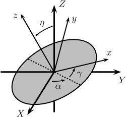
Figure 1: Euler angles relating the Sun frame $\{X,Y,Z\}$ and the orbit frame $\{x,y,z\}$.

	Merc.	Ven.	Earth	Mars	Jup.	Sat.	Ur.	Nept.
$\alpha$	$11.1^{\circ}$	$8.0^{\circ}$	$0^{\circ}$	$3.4^{\circ}$	$3.3^{\circ}$	$6.0^{\circ}$	$1.8^{\circ}$	$3.5^{\circ}$
$\eta$	$28.5^{\circ}$	$24.4^{\circ}$	$23.4^{\circ}$	$24.7^{\circ}$	$23.2^{\circ}$	$22.6^{\circ}$	$23.7^{\circ}$	$22.3^{\circ}$

Table 2: Euler angles of the planets planetangles .

To solve (40), we first seek force-free homogeneous solutions. Several homogeneous solutions exist that can be connected to conventional perturbations to circular orbits. The general homogeneous solution is

$$\delta x_{\rho}^{\text{hom}} = \delta R-R\varepsilon\cos\omega(t-t_{1})$$

$$\delta x_{\varphi}^{\text{hom}} = R\,\delta\varphi-\tfrac{3}{2}\delta R\,\omega t+2R\varepsilon\sin\omega(t-t_{1})\ ,$$

$$\delta x_{z}^{\text{hom}} = R\eta^{\prime}\sin\omega(t-t_{2})\ .$$ (43)

The constant $\delta\varphi$ represents a small translation along the orbit. The constant $\delta R$ gives a transition to a circular orbit that is larger or smaller by $\delta R$. To see this note that while $R$ and $\omega$ may change, the combination $R^{3}\omega^{2}$ is constant for Kepler orbits, so $\delta(R^{3}\omega^{2})=3R^{2}\omega^{2}\delta R+2R^{3}\omega\delta\omega=0$. Using this, we find that the change in position due to a change in radius is $\delta{\boldsymbol{x}}=\delta R\,\hat{\boldsymbol{e}}_{\rho}+R\delta\omega\,t\hat{\boldsymbol{e}}_{\varphi}=\delta R\,\hat{\boldsymbol{e}}_{\rho}-\tfrac{3}{2}\omega t\delta R\,\hat{\boldsymbol{e}}_{\varphi}$, matching the above result. This variation is only valid for sufficiently small times. The constant $\varepsilon$ adds small eccentricity with a pericenter at time $t_{1}$. It can be characterized using an eccentricity vector ${\boldsymbol{\varepsilon}}=\operatorname{Re}\big{(}i\varepsilon e^{-i\omega t_{1}}(\hat{\boldsymbol{e}}_{x}+i\hat{\boldsymbol{e}}_{y})\big{)}$, which has magnitude $\varepsilon$ and points to the pericenter. The perturbations in the position can be written as $\delta x_{\rho}=-R{\boldsymbol{\varepsilon}}\cdot\hat{\boldsymbol{e}}_{\rho},\ \delta x_{\varphi}=-2R{\boldsymbol{\varepsilon}}\cdot\hat{\boldsymbol{e}}_{\varphi}$. Setting $t_{1}$ to one quarter of the orbit period places the pericenter on the $x$ axis. The angle $\eta^{\prime}$ corresponds to a small inclination from the orbit-frame $x$-$y$ plane with the ascending node at time $t_{2}$. Using these results, we can distinguish between conventional perturbations of the orbit and those caused by Lorentz violation.

For the Lorentz-violating inhomogeneous problem, we first consider the $m=0$ and $m=1$ special cases separately since these harmonics also appear in the homogeneous solutions. For $m=0$, we find that $C^{[0]}_{\varphi\rho}=C^{[0]}_{z\rho}=0$. The solution in this case is $\delta x_{\rho}=-\tfrac{1}{3}RC^{[0]}_{\rho\rho}$. This gives a change in the size of the orbit without the corresponding change in the frequency required by Kepler’s third law. The effect mimics a small change in either Newton’s constant $G$ or the source mass. While it may be difficult to detect, this form of Lorentz violation could be sought, in principle, by comparing the third-law constant $R^{3}\omega^{2}$ of different satellites orbiting the same source.

For the $m=\pm 1$ case, two distinct effects arise. We first note that $C^{[1]}_{\rho\rho}=iC^{[1]}_{\varphi\rho}$ and neither of $C^{[1]}_{\rho\rho}$ or $C^{[1]}_{\varphi\rho}$ contain velocity-independent $k=2$ contributions. So only $C^{[1]}_{z\rho}$ gives effects that are unsuppressed by small orbital velocities. Nonetheless, the $C^{[1]}_{\rho\rho}=iC^{[1]}_{\varphi\rho}$ matrix element drives a speed-dependent change in the eccentricity. The inhomogeneous solution can be taken as

$$\delta x_{\rho} = -R\omega t\operatorname{Im}\big{(}C^{[1]}_{\rho\rho}e^{i\omega t}\big{)}$$

$$= -R\omega t\big{|}C^{[1]}_{\rho\rho}\big{|}\cos\omega(t-t_{3})$$

$$\delta x_{\varphi} = -2R\omega t\operatorname{Re}\big{(}C^{[1]}_{\rho\rho}e^{i\omega t}\big{)}$$ (44)

$$= 2R\omega t\big{|}C^{[1]}_{\rho\rho}\big{|}\sin\omega(t-t_{3})$$

where we parameterize the phase as $C^{[1]}_{\rho\rho}=i\big{|}C^{[1]}_{\rho\rho}\big{|}e^{-i\omega t_{3}}$. The above is only valid for small $t$, but the result is an eccentricity that increases a rate of $\dot{\varepsilon}=\omega\big{|}C^{[1]}_{\rho\rho}\big{|}$ with pericenter at time $t_{3}$. The rate of change in the eccentricity vector is

$$\dot{\boldsymbol{\varepsilon}}=\omega\operatorname{Re}\big{(}C^{[1]}_{\rho\rho}(\hat{\boldsymbol{e}}_{x}+i\hat{\boldsymbol{e}}_{y})\big{)}\ .$$ (45)

Note that this will add to the conventional eccentricity vector that may point in a different direction.

The small eccentricities of the planets lead to crude limits on the above effect. As an example, consider the Earth. The eccentricity added per orbit is $2\pi\big{|}C^{[1]}_{\rho\rho}\big{|}$, and the Earth has made roughly $N\approx 4.5\times 10^{9}$ orbits over the age of the Solar System. Taking the Earth’s eccentricity $\varepsilon\approx 0.017$ as an upper bound on the eccentricity due to Lorentz violation, we find the constraint $\big{|}C^{[1]}_{\rho\rho}\big{|}\lesssim\varepsilon/2\pi N\simeq 6\times 10^{-13}$. Since $k=2$ Lorentz violations do not contribute, the dominant effects would likely be from $k=3$, which are linear in speed. Earth’s speed is about $v\approx 10^{-4}$, implying potential sensitivity on the order of $10^{-9}$ to ${c}^{T}_{3jm}$ coefficients. Venus, with its smaller eccentricity and shorter year, is the only planet yielding a slightly better sensitivity.

The $C^{[1]}_{z\rho}$ coefficient combination gives the modification

$$\delta x_{z} = -R\omega t\operatorname{Im}\big{(}C^{[1]}_{z\rho}e^{i\omega t}\big{)}$$ (46)

$$= R\omega t\big{|}C^{[1]}_{z\rho}\big{|}\sin\omega(t-t_{4})\ ,$$

where we parameterize $C^{[1]}_{z\rho}=-\big{|}C^{[1]}_{z\rho}\big{|}e^{-i\omega t_{4}}$. This implies a rotation of the orbital plane at an instantaneous rate of $\Omega=\omega\big{|}C^{[1]}_{z\rho}\big{|}$ about an in-plane axis pointing towards the satellite at time $t_{4}$. We can account for both the rate and the direction by defining a rotation vector

$$\boldsymbol{\Omega}=\omega\operatorname{Im}\big{(}C^{[1]}_{z\rho}(\hat{\boldsymbol{e}}_{x}+i\hat{\boldsymbol{e}}_{y})\big{)}\ .$$ (47)

The orbit axes will gradually rotate according to $\dot{\hat{\boldsymbol{e}}}_{a}=\boldsymbol{\Omega}\times\hat{\boldsymbol{e}}_{a}$. The resulting secular variations in the Euler angles are

$$\dot{\alpha} = \omega\frac{\sin\gamma\operatorname{Im}C^{[1]}_{z\rho}+\cos\gamma\operatorname{Re}C^{[1]}_{z\rho}}{\sin\eta}\ ,$$

$$\dot{\eta} = \omega\big{(}\cos\gamma\operatorname{Im}C^{[1]}_{z\rho}-\sin\gamma\operatorname{Re}C^{[1]}_{z\rho}\big{)}\ ,$$

$$\dot{\gamma} = -\cos\eta\,\dot{\alpha}\ .$$ (48)

Note that the $C^{[1]}_{z\rho}$ coefficient combination also depends on the Euler angles. A demonstration of the above rotation is provided in Ref. clyburn , where the effects of $d=4$ violations on binary systems are simulated.

Assuming a small net effect, we can approximate the total rotation of the orbital plane after $N$ orbits as $2\pi N\big{|}C^{[1]}_{z\rho}\big{|}$. Given that the orbital planes of the eight planets and the Sun’s equator all differ by no more than about $10^{\circ}$, we take this as an upper bound on the change in inclination for each planet over the age of the Solar System. Mercury, with its short year, then produces the tightest constraint, $\big{|}C^{[1]}_{z\rho}\big{|}\lesssim 1.5\times 10^{-12}$. Unlike the change in eccentricity, velocity-independent $k=2$ violations contribute to the change in inclination. So planetary orbits could constrain ${c}^{T}_{22m}$ quadrupole coefficients at the level of $10^{-12}$. The different orientations of the different orbits could in principle be used to access different combinations of coefficients. However, the small inclinations imply the effects of Lorentz violation on all planets depend on similar combinations, reducing the sensitivity to the additional coefficient space accessible through a combined analysis.

Planetary ephemerides could be used to place more rigorous bounds at levels comparable to the simple estimate given above. For example, limits on the evolution of planetary orbits have been shown to constrain the dimensionless $\bar{s}^{\mu\nu}$ coefficients in the pure-gravity sector of the SME down to parts in $10^{12}$ iorio ; hees . Lunar laser ranging has also been used to test Lorentz symmetry in gravity llr1 ; llr2 and in matter-gravity couplings llr3 down to parts in $10^{12}$. The $\bar{s}^{\mu\nu}$ coefficients produce effects similar to those found above qbk06 , and we expect similar constraints on ${c}^{T}_{22m}$ coefficients. This implies sensitivities at the level of $\sim 10^{-12}\text{ GeV}^{4-d}$ to ${a^{\prime}_{npe}}^{(d)}_{kjm}$ and ${c^{\prime}_{npe}}^{(d)}_{kjm}$ SME coefficient combinations.

Binary pulsars provide another test of Lorentz invariance in orbital dynamics qbk06 ; jennings . These systems have been used to test Lorentz invariance to parts in $10^{11}$ in gravity shao_grav1 ; shao_grav2 and matter-gravity couplings shao_matter . They’ve also been used to search for velocity-dependent effects from dimension $d=5$ terms shao_d5 and from $d=8$ cubic terms in the gravity sector of the SME shao_d8 . We also note that Lorentz violation can be constrained with non-binary pulsars pulsar1 ; pulsar2 . Binary pulsar are unique among orbital tests in that they provide clean access to neutron coefficients for Lorentz violation and are therefore complementary to tests involving ordinary matter.

The perturbations driven at higher frequencies with $m>1$ are

$$\delta x_{\rho} = -\frac{2R}{m^{2}(m^{2}-1)}\operatorname{Re}\Big{(}\big{(}m^{2}C^{[m]}_{\rho\rho}-2imC^{[m]}_{\varphi\rho}\big{)}e^{im\omega t}\Big{)}\ ,$$

$$\delta x_{\varphi} = -\frac{2R}{m^{2}(m^{2}-1)}\operatorname{Re}\Big{(}\big{(}(3+m^{2})C^{[m]}_{\varphi\rho}+2imC^{[m]}_{\rho\rho}\big{)}e^{im\omega t}\Big{)}\ ,$$

$$\delta x_{z} = -\frac{2R}{m^{2}-1}\operatorname{Re}\Big{(}C^{[m]}_{z\rho}e^{im\omega t}\Big{)}\ .$$ (49)

Unlike the $m=1$ case, which gave a secular evolution of the orbit, violations with $m\geq 2$ produce periodic deviations from the conventional orbit. For example, $\delta x_{z}$ produces periodic oscillations about of the average orbital plane. Among the effects from $\delta x_{\rho}$ and $\delta x_{\varphi}$ displacements is a time-dependent change in the areal velocity $\delta\dot{A}=R\omega\delta x_{\rho}+\tfrac{1}{2}R\delta\dot{x}_{\varphi}=R^{2}\omega m^{-1}\operatorname{Im}\big{(}C^{[m]}_{\varphi\rho}e^{im\omega t}\big{)}$, violating Kepler’s second law. Again, these periodic variations are similar to ones arising in the gravity sector of the SME qbk06 and could be sought in planetary motion or in lunar laser ranging. Note that since $k\geq j\geq|m|$, the effects of Lorentz violation at frequencies greater than $2\omega$ necessarily involve the orbital speed of the satellite. Consequently, unsuppressed speed-independent periodic variations only arise at twice the orbital frequency.

3.3 Acoustic Resonators

This section considers the effects of Lorentz violation in continuous media with particular focus on acoustic resonances in piezoelectric materials. For continuous media, the Lorentz-violating hamiltonian density can be taken as

$$\delta{\mathcal{H}}=-\sum_{kjm}\rho^{1-k}|{\boldsymbol{{\mathcal{P}}}}|^{k}Y_{jm}(\hat{\boldsymbol{{\mathcal{P}}}})\,{c}^{T}_{kjm}\ ,$$ (50)

where $\rho$ is the mass density of the material, ${\boldsymbol{{\mathcal{P}}}}$ is the momentum density, and $\hat{\boldsymbol{{\mathcal{P}}}}={\boldsymbol{{\mathcal{P}}}}/|{\boldsymbol{{\mathcal{P}}}}|$. Using the above, we can find modifications to the Hamilton equations of motion. Alternatively, we could instead employ a lagrangian approach, where the leading-order change to the Lagrange density can be taken as

$$\delta{\cal L}=\sum_{kjm}\rho|{\boldsymbol{v}}|^{k}Y_{jm}(\hat{\boldsymbol{v}})\,{c}^{T}_{kjm}\ ,$$ (51)

where ${\boldsymbol{v}}={\boldsymbol{v}}({\boldsymbol{x}},t)$ is the local velocity of the medium, and $\hat{\boldsymbol{v}}={\boldsymbol{v}}/|{\boldsymbol{v}}|$. Denoting the mechanical displacement of the medium at equilibrium position ${\boldsymbol{x}}$ in a body-fixed frame as ${\boldsymbol{u}}={\boldsymbol{u}}({\boldsymbol{x}},t)$, the velocity is then given by ${\boldsymbol{v}}=\dot{\boldsymbol{u}}$. Note that ${\boldsymbol{v}}\approx{\boldsymbol{{\mathcal{P}}}}/\rho$, but differs slightly from the usual result due to Lorentz violation.

The conventional Lagrange density for a piezoelectric material is given by

$${\cal L}=\tfrac{1}{2}\rho\dot{{\boldsymbol{u}}}^{2}-\tfrac{1}{2}{\mathcal{S}}^{abcd}u^{a}_{,b}u^{c}_{,d}+\tfrac{1}{2}\epsilon^{ab}\phi_{,a}\phi_{,b}-e^{abc}\phi_{,a}u^{b}_{,c}\ ,$$ (52)

where $u^{a}_{,b}=\partial u^{a}/\partial x^{b}$ are spatial derivatives of the displacements $u^{a}$, $\phi_{,a}=\partial\phi/\partial x^{a}$ is the gradient of the electric potential $\phi$, ${\mathcal{S}}^{abcd}$ is the stiffness tensor, $\epsilon^{ab}$ is the permittivity tensor, and $e^{abc}$ is the piezoelectric tensor. The stiffness tensor ${\mathcal{S}}^{abcd}$ is taken to be symmetric in the first pair of indices and the last pair of indices and symmetric under interchange of the pairs, giving twenty-one independent components. The permittivity tensor $\epsilon^{ab}$ is symmetric, and the piezoelectric tensor $e^{abc}$ is symmetric in the last two indices. The equations of motion for the system including Lorentz violation are given by

$$\rho\ddot{u}^{a}+\rho C^{ab}\ddot{u}^{b}=T^{ab}_{,b}\ ,\quad 0=D^{a}_{,a}\ ,$$ (53)

where $T^{ab}={\mathcal{S}}^{abcd}u^{c}_{,d}+e^{cab}\phi_{,c}$ is the stress tensor, $D^{a}=-\epsilon^{ab}\phi_{,b}+e^{abc}u^{b}_{,c}$ is the electric displacement field, and $C^{ab}$ is the Lorentz-violating tensor from (24) evaluated at velocity ${\boldsymbol{v}}=\dot{{\boldsymbol{u}}}$.

Periodic solutions to (53) can be found using methods similar to those used for orbits. Solutions with period $2\pi/\omega$ will in general includes various harmonics of the fundamental frequency $\omega$. To find them, first expand each variable in Fourier modes: ${\boldsymbol{u}}=\sum_{m}{\boldsymbol{u}}^{[m]}e^{im\omega t}$, $\phi=\sum_{m}\phi^{[m]}e^{im\omega t}$, and $C^{ab}=\sum_{m}C^{[m]ab}e^{im\omega t}$. The equations of motion (53) lead to a set of coupled equations relating the various Fourier components, which can be solved perturbatively. However, we are primarily interested in changes to the frequency $\omega$, which can be found using a simpler method.

We begin by assuming the solution with Lorentz violation ${\boldsymbol{u}}$ has frequency and amplitudes that are close to those for a conventional solution ${\boldsymbol{u}}_{0}$. Manipulating the equations of motion for ${\boldsymbol{u}}$ and ${\boldsymbol{u}}_{0}$, one can show the relation

$$\rho\int_{V}d^{3}x\,\big{(}\ddot{{\boldsymbol{u}}}\cdot{\boldsymbol{u}}_{0}+\ddot{{\boldsymbol{u}}}\cdot C\cdot{\boldsymbol{u}}_{0}-{\boldsymbol{u}}\cdot\ddot{{\boldsymbol{u}}}_{0}\big{)}=\int_{\partial V}d{\boldsymbol{\sigma}}\cdot\big{(}T\cdot{\boldsymbol{u}}_{0}-T_{0}\cdot{\boldsymbol{u}}-{\boldsymbol{D}}_{0}\phi+{\boldsymbol{D}}\phi_{0}\big{)}\ ,$$ (54)

where the left-hand side is integrated over the volume $V$ of the resonator, and the right-hand side is integrated over the surface $\partial V$. The conventional stress tensor $T_{0}$ depends on ${\boldsymbol{u}}_{0}$, the conventional potential $\phi_{0}$, and the conventional displacement field ${\boldsymbol{D}}_{0}$. We then assume the surface terms vanish, giving

$$\int_{V}d^{3}x\,\big{(}\ddot{\boldsymbol{u}}\cdot{\boldsymbol{u}}_{0}-{\boldsymbol{u}}\cdot\ddot{\boldsymbol{u}}_{0}\big{)}=-\int_{V}d^{3}x\,\ddot{\boldsymbol{u}}\cdot C\cdot{\boldsymbol{u}}_{0}\ .$$ (55)

Assuming simple harmonic conventional solutions, this expression oscillates at frequencies $m\omega\pm\omega_{0}=(m\pm 1)\omega_{0}+m\delta\omega$, where $\delta\omega=\omega-\omega_{0}$ is the shift in the fundamental frequency from the usual frequency $\omega_{0}$. Writing the amplitudes as ${\boldsymbol{u}}^{[m]}={\boldsymbol{u}}_{0}^{[m]}+\delta{\boldsymbol{u}}^{[m]}$, where $\delta{\boldsymbol{u}}^{[m]}$ is the change due to Lorentz violation, we can expand the frequency components of (55) in small parameters depending on coefficients for Lorentz violation. The zeroth-order equations are identically satisfied. The first-order equations give

$$\int_{V}d^{3}x\,\big{(}(1-m^{2})\delta{\boldsymbol{u}}^{[m]}\cdot{\boldsymbol{u}}_{0}^{[\pm 1]}-2m^{2}\frac{\delta\omega}{\omega_{0}}\,{\boldsymbol{u}}_{0}^{[m]}\cdot{\boldsymbol{u}}_{0}^{[\pm 1]}\big{)}=\int_{V}d^{3}x\,\sum_{m^{\prime}}{m^{\prime}}^{2}{\boldsymbol{u}}_{0}^{[m^{\prime}]}\cdot C^{[m-m^{\prime}]}\cdot{\boldsymbol{u}}_{0}^{[\pm 1]}\ .$$ (56)

Note that ${\boldsymbol{u}}_{0}^{[m]}=0$ for $m\neq\pm 1$ since we assume ${\boldsymbol{u}}_{0}$ is simple harmonic. The shift in frequency $\delta\omega$ can be isolated by taking $m=\mp 1$, which gives

$$\frac{\delta\omega}{\omega_{0}} \approx -\frac{1}{2}\frac{\int_{V}d^{3}x\,\big{(}{\boldsymbol{u}}_{0}^{[-1]}\cdot C^{[0]}\cdot{\boldsymbol{u}}_{0}^{[1]}+{\boldsymbol{u}}_{0}^{[1]}\cdot C^{[-2]}\cdot{\boldsymbol{u}}_{0}^{[1]}\big{)}}{\int_{V}d^{3}x\,{\boldsymbol{u}}_{0}^{[1]}\cdot{\boldsymbol{u}}_{0}^{[-1]}}$$ (57)

$$= -\frac{1}{2}\frac{\int_{V}d^{3}x\,\langle{{\boldsymbol{u}}_{0}\cdot C\cdot{\boldsymbol{u}}_{0}}\rangle_{t}}{\int_{V}d^{3}x\,\langle{{\boldsymbol{u}}_{0}\cdot{\boldsymbol{u}}_{0}}\rangle_{t}}\ ,$$

where brackets $\langle{}\rangle_{t}$ indicate the time average. The $C$ tensor in this expression is calculated using the conventional velocity ${\boldsymbol{v}}_{0}=\dot{\boldsymbol{u}}_{0}$. The leading-order frequency shift is then completely determined by the coefficients for Lorentz violation and the usual solution ${\boldsymbol{u}}_{0}$.

The time averages in (57) may be difficult to calculate in general but are relatively simple in the case of standing waves with local linear polarization, where we can take ${\boldsymbol{u}}_{0}({\boldsymbol{x}},t)\rightarrow{\boldsymbol{u}}_{0}({\boldsymbol{x}})\sin(\omega_{0}t)$. The velocity is replaced with ${\boldsymbol{v}}_{0}({\boldsymbol{x}},t)\rightarrow\omega_{0}{\boldsymbol{u}}({\boldsymbol{x}})\cos(\omega_{0}t)$ and is parallel to the displacement ${\boldsymbol{u}}_{0}({\boldsymbol{x}})$. The time average in the denominator of (57) becomes $\langle{{\boldsymbol{u}}_{0}\cdot{\boldsymbol{u}}_{0}}\rangle_{t}\rightarrow\tfrac{1}{2}{\boldsymbol{u}}_{0}^{2}$. The numerator can be shown to vanish for odd values of $k$. For fixed even values of $k$, the time average in the numerator becomes

$$\langle{{\boldsymbol{u}}_{0}\cdot C\cdot{\boldsymbol{u}}_{0}}\rangle_{t} \rightarrow \langle{\sin^{2}(\omega_{0}t)\cos^{k-2}(\omega_{0}t)}\rangle_{t}\,{\boldsymbol{u}}_{0}\cdot C(\omega_{0}{\boldsymbol{u}}_{0})\cdot{\boldsymbol{u}}_{0}$$ (58)

$$= \frac{(k-3)!!}{k!!}{\boldsymbol{u}}_{0}\cdot C(\omega_{0}{\boldsymbol{u}}_{0})\cdot{\boldsymbol{u}}_{0}$$

The frequency shift is then given by

$$\frac{\delta\omega}{\omega_{0}}\approx-\sum_{kjm}\omega_{0}^{k-2}\frac{(k-1)!!}{(k-2)!!}\frac{\int_{V}d^{3}x\,|{\boldsymbol{u}}_{0}|^{k}Y_{jm}(\hat{\boldsymbol{u}}_{0})}{\int_{V}d^{3}x\,|{\boldsymbol{u}}_{0}|^{2}}{c}^{T,\text{lab}}_{kjm}$$ (59)

where $k$ is restricted to even values $k\geq 2$, and ${c}^{T,\text{lab}}_{kjm}$ are laboratory-frame coefficients. The dimensionless factors multiplying the ${c}^{T}_{kjm}$ coefficients determine the sensitivity of an acoustic-resonator experiment. Assuming oscillation amplitudes on the order of 100 angstrom and frequencies on the order of a MHz, these factors scale as $\sim 10^{-10(k-2)}$. This drastically reduces the sensitivity to violations with $k\neq 2$. We therefore focus on the $k=2$ case. The problem simplifies even further for cases in which the vibration direction $\hat{\boldsymbol{u}}_{0}({\boldsymbol{x}})$ is relatively constant over the volume of the resonator:

$$\frac{\delta\omega}{\omega_{0}} \approx -\sum_{jm}Y_{jm}(\hat{\boldsymbol{u}}_{0})\,{c}^{T,\text{lab}}_{2jm}$$ (60)

$$\approx \tfrac{1}{2}\sum_{dljm}M_{n}^{d-4}\left(\begin{smallmatrix}(d+2l-5)/2\\ l\end{smallmatrix}\right)Y_{jm}(\hat{\boldsymbol{u}}_{0})\,\big{(}{a^{\prime}_{npe}}^{(d)\text{lab}}_{(2-2l)jm}-{c^{\prime}_{npe}}^{(d)\text{lab}}_{(2-2l)jm}\big{)}\ ,$$

assuming in the last line that the medium is comprised of roughly equal numbers of neutrons, protons, and electrons. The frequency shift is then limited to quadrupole $j=2$ and isotropic $j=0$ violations.

The rotational and orbital motion of the Earth implies that the laboratory frame is noninertial. As a result, the laboratory-frame coefficients will change as the orientation and velocity of the laboratory changes, producing periodic variations in the frequency shift. We account for these changes using the transformation between the laboratory frame and Sun-centered frame discussed in Section 2.3. The rotations introduce sidereal variations in the laboratory-frame coefficients. The coefficients also vary with the angle of the resonator in the laboratory. In experiments involving rotating turntables, this produces variations at the turn rate. Annual changes in the velocity of Earth lead to annual variations in the signal. These, however, enter through boosts and are suppressed by the boost velocity $\beta\approx 10^{-4}$ relative to the other variations.

The fluctuations in the frequency shift take the form

$$\frac{\delta\omega}{\omega_{0}}=\sum_{{m_{\text{r}}}{m_{\text{s}}}{m_{\text{a}}}}A_{{m_{\text{r}}}{m_{\text{s}}}{m_{\text{a}}}}e^{i{m_{\text{r}}}\varphi+i{m_{\text{s}}}\omega_{\oplus}T_{\oplus}+i{m_{\text{a}}}\Omega_{\oplus}T}\ ,$$ (61)

where $\omega_{\oplus}=2\pi/\text{23hr 56min}$ and $\Omega_{\oplus}=2\pi/\text{1yr}$ are respectively the sidereal and annual frequencies. The time $T_{\oplus}$ is defined so that the laboratory zenith points at right ascension $\alpha=0$ when $T_{\oplus}=0$, and time $T=0$ at the vernal equinox. The angle $\varphi$ is between the laboratory-frame $x$ axis and south. The laboratory frame is fixed to the resonator, which may be affixed to a turntable. In this case, $\varphi$ changes at the turntable rotation rate ${\omega_{\text{r}}}$. The indices ${m_{\text{r}}}$, ${m_{\text{s}}}$, and ${m_{\text{a}}}$ are the harmonic numbers for variations at respectively the turntable rotation frequency ${\omega_{\text{r}}}$, sidereal frequency $\omega_{\oplus}$, and annual frequency $\Omega_{\oplus}$. The amplitudes obey the relation $A^{*}_{{m_{\text{r}}}{m_{\text{s}}}{m_{\text{a}}}}=A_{(-{m_{\text{r}}})(-{m_{\text{s}}})(-{m_{\text{a}}})}$, ensuring that the frequency shift is real.

Applying the Lorentz transformations outlined in Section 2.3 to the laboratory-frame coefficients in (60), we find that the modulation amplitudes due to rotations only are

$$A_{{m_{\text{r}}}{m_{\text{s}}}({m_{\text{a}}}=0)}=\tfrac{1}{2}\sum_{dlj}M_{n}^{d-4}\left(\begin{smallmatrix}(d+2l-5)/2\\ l\end{smallmatrix}\right)Y_{j{m_{\text{r}}}}(\hat{\boldsymbol{u}}_{0})\,d^{(j)}_{{m_{\text{r}}}{m_{\text{s}}}}(-\chi)\,\Big{(}{a^{\prime}_{npe}}^{(d)}_{(2-2l)j{m_{\text{s}}}}-{c^{\prime}_{npe}}^{(d)}_{(2-2l)j{m_{\text{s}}}}\Big{)}\ ,$$ (62)

in terms of the Sun-frame ${a^{\prime}_{npe}}^{(d)}_{kjm}$ and ${c^{\prime}_{npe}}^{(d)}_{kjm}$ coefficients. The isotropic $j=0$ violations produce a constant shift. The quadrupole $j=2$ violations give variations at frequencies ${m_{\text{r}}}{\omega_{\text{r}}}+{m_{\text{s}}}\omega_{\oplus}$ up to the second harmonic in both the turntable and sidereal rates: $|{m_{\text{r}}}|,|{m_{\text{s}}}|\leq 2$. Note, however, that $|{m_{\text{r}}}|=1$ variations will be absent in oscillators with horizontal or vertical vibrations.

Including leading-order boost effects due to the orbital motion of the Earth gives variations at frequencies ${m_{\text{r}}}{\omega_{\text{r}}}+{m_{\text{s}}}\omega_{\oplus}+{m_{\text{a}}}\Omega_{\oplus}$ with ${m_{\text{a}}}=\pm 1$. The amplitudes for these are given by

$$A_{{m_{\text{r}}}{m_{\text{s}}}({m_{\text{a}}}=\pm 1)} = \tfrac{1}{2}\sum_{dlj}M_{n}^{d-4}\left(\begin{smallmatrix}(d+2l-5)/2\\ l\end{smallmatrix}\right)Y_{j{m_{\text{r}}}}(\hat{\boldsymbol{u}}_{0})\,d^{(j)}_{{m_{\text{r}}}{m_{\text{s}}}}(-\chi)\,$$ (63)

$$\qquad\times\sum_{k^{\prime}j^{\prime}m^{\prime}m^{\prime\prime}}\Gamma^{(d)k^{\prime}j^{\prime}m^{\prime}m^{\prime\prime}}_{(2-2l)j{m_{\text{s}}}}\,B_{m^{\prime\prime}{m_{\text{a}}}}\Big{(}{a^{\prime}_{npe}}^{(d)}_{k^{\prime}j^{\prime}m^{\prime}}-{c^{\prime}_{npe}}^{(d)}_{k^{\prime}j^{\prime}m^{\prime}}\Big{)}\ ,$$

where the numerical $\Gamma^{(d)k^{\prime}j^{\prime}m^{\prime}m^{\prime\prime}}_{(2-2l)j{m_{\text{s}}}}$ constants are given in (35), and the $B_{m^{\prime\prime}{m_{\text{a}}}}$ boost factors are in (36). This gives sensitivity to other coefficients for Lorentz violation but at levels suppressed by the small boost velocity $\beta\approx 10^{-4}$ of the Earth.

Searches for Lorentz violation in quartz resonators have demonstrated sensitivities on the order of parts in $10^{14}$ to $d=4$ violations quartz1 and are expected to improve by two orders of magnitude quartz2 . We therefore expect sensitivities near $10^{-16}\text{ GeV}^{4-d}$ to the dimension-$d$ combinations ${a^{\prime}_{npe}}^{(d)}_{2jm}$ and ${c^{\prime}_{npe}}^{(d)}_{2jm}$.

4 Summary

A violation of Lorentz invariance would necessarily indicate new physics with potential origins in quantum gravity. High-precision experiments have limited violations in a large variety of systems tables . In this paper, we derive the effects of Lorentz violation on dynamics of ordinary matter. We include all linear dimension-$d$ violations in the electrons, protons, and neutrons, excluding violations involving electromagnetic and gravitational interactions.

The effective hamiltonian for a macroscopic test body is derived in Section 2.1. The Lorentz-violating contributions are given in (12) in terms of macroscopic coefficients for Lorentz violation ${c}^{T}_{kjm}$. Equation (14) relates these coefficients to underlying SME coefficients for electrons, protons, and neutrons. Ignoring internal kinetic energy, the result reduces to (15). Equation (16) gives ${c}^{T}_{kjm}$ for matter with equal numbers electrons and protons, and (18) is for matter with equal numbers of electrons, protons, and neutrons. The equations of motion are discussed in Section 2.2. A modified Newton’s second law is given in (23). Section 2.3 discusses observer Lorentz transformations of the coefficients, relating coefficients in the Sun-centered equatorial frame to a standard laboratory frame. The boosts are calculated to first order in velocity, resulting in (37).

Section 3 contains several applications. Tests of the the weak equivalence principle are discussed in Section 3.1, including tests involving free-fall experiments ff87 ; ff89 ; ff90 ; ff92 ; ff96 , the space-based MICROSCOPE experiment microscope and torsion-balance experiments Roll ; Braginskii ; Adelberger ; Su ; Schlamminger . Implied bounds on isotropic Lorentz violation from these experiments are given in Table 1, demonstrating sensitivities down to $\sim 10^{-13}\text{ GeV}^{4-d}$ to dimension $d$ violations.

Planetary orbits are discussed in Section 3.2. The effects of Lorentz violation include a drift in eccentricity, a rotation of the orbital plane, and periodic variations about conventional orbits. The small eccentricities of Earth and Venus limit Lorentz violation at the $\sim 10^{-9}\text{ GeV}^{4-d}$ level. The approximate alignment of the planets’ orbital planes leads to bounds of $\sim 10^{-12}\text{ GeV}^{4-d}$. Improvements on these rough constraints are expected in detailed studies of planetary ephemerides iorio ; hees and through lunar laser ranging llr1 ; llr2 ; llr3 . Binary pulsars offer another promising area of study that is particularly sensitive to Lorentz violations in neutrons qbk06 ; jennings ; shao_grav1 ; shao_grav2 ; shao_matter ; shao_d5 ; shao_d8 .

Section 3.3 gives the Lorentz-violating Lagrange density for continuous media (51). The shift in resonant frequency in piezoelectric acoustic resonators is calculated, including boost effects. The shifts vary periodically at frequencies involving the the turntable rotation rate, the Earth’s sidereal rotation rate, and the Earth’s orbital frequency. Experiments have demonstrated sensitivities at parts in $10^{14}$ to dimension $d=4$ Lorentz violations quartz1 and are expected to reach $10^{-16}\text{ GeV}^{4-d}$ to arbitrary dimension $d$ violations quartz2 .

These results show that extreme precision can be achieve in studies of spacetime symmetries in macroscopic matter. While not as sensitive as the best of the microscopic tests atomse1 ; atomse2 ; atomse3 ; atomspn1 ; atomspn2 , experiments involving ordinary matter rely on different assumptions and may provide access to different combinations of SME coefficients and therefore represent a powerful tool in our search for new physics.

This research was funded by the United States National Science Foundation grant number PHY-1819412.

The author declares no conflicts of interest.

no

Appendix A

This Appendix derives the symmetric product identity for spherical-harmonic tensors. See Ref. Yrjm for a detailed discussion of the ${\mathcal{Y}}^{\varrho}_{jm}$ tensors and the notation used here.

Expanding the symmetric product of two spherical-harmonic tensors in the basis of spherical-harmonic tensors, we can write

$${\mathcal{Y}}^{\varrho_{1}}_{j_{1}m_{1}}\odot{\mathcal{Y}}^{\varrho_{2}}_{j_{2}m_{2}}=\sum_{JM}{{\mathcal{A}}^{\varrho_{1}\varrho_{2}}_{j_{1}m_{1}j_{2}m_{2}JM}}{\mathcal{Y}}^{(\varrho_{1}+\varrho_{2})}_{JM}\ .$$ (64)

The ${{\mathcal{A}}^{\varrho_{1}\varrho_{2}}_{j_{1}m_{1}j_{2}m_{2}JM}}$ coefficients are nonzero for the usual angular-momentum-addition relations $M=m_{1}+m_{2}$ and $j_{1}+j_{2}\geq J\geq|j_{1}-j_{2}|$ and for $j_{1}+j_{2}-J=\text{even}$. The nonzero values are real and given by

$${{\mathcal{A}}^{\varrho_{1}\varrho_{2}}_{j_{1}m_{1}j_{2}m_{2}JM}} = {\mathcal{Y}}^{(\varrho_{1}+\varrho_{2})*}_{JM}\cdot({\mathcal{Y}}^{\varrho_{1}}_{j_{1}m_{1}}\odot{\mathcal{Y}}^{\varrho_{2}}_{j_{2}m_{2}})$$

$$= (2J+1)(J+M)!(J-M)!\frac{{{\mathcal{B}}^{\varrho_{1}+\varrho_{2}}_{JM}}}{{{\mathcal{B}}^{\varrho_{1}}_{j_{1}m_{1}}}{{\mathcal{B}}^{\varrho_{2}}_{j_{2}m_{2}}}}$$

$$\times\tfrac{(j_{1}+j_{2}-J-1)!!(j_{1}-j_{2}+J-1)!!(j_{2}-j_{1}+J-1)!!}{(j_{1}+j_{2}+J+1)!!}$$

$$\times\sum_{n}\tfrac{(-1)^{n}}{n!(n+J-j_{2}-m_{1})!(n+J-j_{1}+m_{2})!(j_{1}+j_{2}-J-n)!(j_{1}+m_{1}-n)!(j_{2}-m_{2}-n)!}\ ,$$

where the sum is limited to $n$ values that give nonnegative arguments in all factorials, and we define

$${{\mathcal{B}}^{\varrho}_{jm}}=(-1)^{j/2}\sqrt{\tfrac{(\varrho+j+1)!!(\varrho-j)!!}{(2j+1)\varrho!(j+m)!(j-m)!}}\ ,$$ (66)

for convenience.

Our derivation starts by considering the vector

$$\boldsymbol{\xi}=\frac{i\zeta}{\sqrt{2}}\hat{\boldsymbol{e}}_{\text{\scalebox{0.8}{$\uparrow$}}}+\frac{i}{\sqrt{2}\zeta}\hat{\boldsymbol{e}}_{\text{\scalebox{0.8}{$\downarrow$}}}+\hat{\boldsymbol{e}}_{z}$$ (67)

for arbitrary complex number $\zeta$. The unit vectors $\hat{\boldsymbol{e}}_{\text{\scalebox{0.8}{$\uparrow$}}}=(\hat{\boldsymbol{e}}_{x}+i\hat{\boldsymbol{e}}_{y})/\sqrt{2}$, $\hat{\boldsymbol{e}}_{\text{\scalebox{0.8}{$\downarrow$}}}=(\hat{\boldsymbol{e}}_{x}-i\hat{\boldsymbol{e}}_{y})/\sqrt{2}$, and $\hat{\boldsymbol{e}}_{z}$ form a spin-eigenbasis for quantization along the $z$ axis. A short calculation reveals that the $j$-fold symmetric product of $\boldsymbol{\xi}$ is

$$\boldsymbol{\xi}^{\,\odot j}=\sum_{m}C_{jm}\zeta^{m}{\mathcal{Y}}_{jm}\ ,$$ (68)

where ${\mathcal{Y}}_{jm}={\mathcal{Y}}^{j}_{jm}$ are the traceless spherical-harmonic tensors, and

$$C_{jm}=(-i)^{m}\sqrt{\tfrac{j!(2j-1)!!}{(j+m)!(j-m)!}}$$ (69)

for $|m|\leq j$. The symmetric product in (68) serves as a generating function for the traceless spherical-harmonic tensors. Note that $\boldsymbol{\xi}\cdot\boldsymbol{\xi}=0$, which confirming that it is traceless.

Next consider the inner product

$$\boldsymbol{\xi}^{\,\odot J}\cdot({\mathcal{Y}}_{j_{1}m_{1}}^{*}\odot{\mathcal{Y}}_{j_{2}m_{2}}^{*})=(\boldsymbol{\xi}^{\,\odot j_{1}}\cdot{\mathcal{Y}}_{j_{1}m_{1}}^{*})(\boldsymbol{\xi}^{\,\odot j_{2}}\cdot{\mathcal{Y}}_{j_{2}m_{2}}^{*})\ ,$$ (70)

where $J=j_{1}+j_{2}$. The two sides of this equation evaluate to

$$\sum_{M}C_{JM}\zeta^{M}{\mathcal{Y}}_{JM}\cdot({\mathcal{Y}}_{j_{1}m_{1}}^{*}\odot{\mathcal{Y}}_{j_{2}m_{2}}^{*})=C_{j_{1}m_{1}}C_{j_{2}m_{2}}\zeta^{m_{1}+m_{2}}\ ,$$ (71)

which implies

$${\mathcal{Y}}_{JM}\cdot({\mathcal{Y}}_{j_{1}m_{1}}^{*}\odot{\mathcal{Y}}_{j_{2}m_{2}}^{*})=\delta_{M,m_{1}+m_{2}}\frac{C_{j_{1}m_{1}}C_{j_{2}m_{2}}}{C_{JM}}\ .$$ (72)

The complex conjugate of this gives the ${{\mathcal{A}}^{j_{1}j_{2}}_{j_{1}m_{1}j_{2}m_{2}JM}}$ coefficients for traceless tensors.

To find the inner product for tensors of nonzero trace, we consider traces of the product

$$\boldsymbol{\xi}_{1}^{\odot j_{1}}\odot\boldsymbol{\xi}_{2}^{\odot j_{2}}=\sum_{m_{1}m_{2}}C_{j_{1}m_{1}}C_{j_{1}m_{1}}\zeta_{1}^{m_{1}}\zeta_{2}^{m_{2}}{\mathcal{Y}}_{j_{1}m_{1}}\odot{\mathcal{Y}}_{j_{2}m_{2}}\ .$$ (73)

Using $\boldsymbol{\xi}_{1}\cdot\boldsymbol{\xi}_{2}=-(\zeta_{1}-\zeta_{2})^{2}/2\zeta_{1}\zeta_{2}$, one can show that taking $N$ traces gives

$$(-\zeta_{1}\zeta_{2})^{N}g^{\odot N}\cdot(\boldsymbol{\xi}_{1}^{\odot j_{1}}\odot\boldsymbol{\xi}_{2}^{\odot j_{2}})=\frac{j_{1}^{\underline{N}}j_{2}^{\underline{N}}}{(j_{1}+j_{2})^{\underline{2N}}}(\zeta_{1}-\zeta_{2})^{2N}\boldsymbol{\xi}_{1}^{\odot(j_{1}-N)}\odot\boldsymbol{\xi}_{2}^{\odot(j_{2}-N)}\ ,$$ (74)

where $g$ is the euclidean metric, and $x^{\underline{n}}$ indicates the falling factorial. Matching terms by their powers in $\xi_{1}$ and $\xi_{2}$, we find

$$g^{\odot N}\cdot({\mathcal{Y}}_{j_{1}m_{1}}\odot{\mathcal{Y}}_{j_{2}m_{2}}) = \frac{(2N)!(-1)^{N}j_{1}^{\underline{N}}j_{2}^{\underline{N}}}{(j_{1}+j_{2})^{\underline{2N}}C_{j_{1}m_{1}}C_{j_{2}m_{2}}}\sum_{n=0}^{2N}\tfrac{(-1)^{n}}{n!(2N-n)!}C_{(j_{1}-N)(m_{1}+N-n)}C_{(j_{2}-N)(m_{2}-N+n)}$$ (75)

$$\times{\mathcal{Y}}_{(j_{1}-N)(m_{1}+N-n)}\odot{\mathcal{Y}}_{(j_{2}-N)(m_{2}-N+n)}\ .$$

Finally, the identities

$${\mathcal{Y}}^{\varrho}_{jm} = {{\mathcal{D}}^{\varrho}_{j}}{\mathcal{Y}}_{jm}\odot g^{\odot\frac{1}{2}(\varrho-j)}\ ,$$

$${{\mathcal{D}}^{\varrho}_{j}}g^{\odot N}\cdot{\mathcal{Y}}^{\varrho}_{jm} = {{\mathcal{D}}^{\varrho-2N}_{j}}{\mathcal{Y}}^{\varrho-2N}_{jm}\ ,$$ (76)

where

$${{\mathcal{D}}^{\varrho}_{j}}=\sqrt{\tfrac{\varrho!(2j+1)!!}{j!(\varrho+j+1)!!(\varrho-j)!!}}\ ,$$ (77)

can be used to show that

$${{\mathcal{D}}^{\varrho_{1}+\varrho_{2}}_{J}}{\mathcal{Y}}^{(\varrho_{1}+\varrho_{2})*}_{JM}\cdot({\mathcal{Y}}^{\varrho_{1}}_{j_{1}m_{1}}\odot{\mathcal{Y}}^{\varrho_{2}}_{j_{2}m_{2}})={{\mathcal{D}}^{\varrho_{1}}_{j_{1}}}{{\mathcal{D}}^{\varrho_{2}}_{j_{2}}}{{\mathcal{D}}^{j_{1}+j_{2}}_{J}}{{\mathcal{D}}^{j_{1}+j_{2}}_{J}}{\mathcal{Y}}_{JM}^{*}\cdot\big{(}g^{\odot\frac{1}{2}(j_{1}+j_{2}-J)}\cdot({\mathcal{Y}}_{j_{1}m_{2}}\odot{\mathcal{Y}}_{j_{2}m_{2}})\big{)}\ .$$ (78)

Combining (78) with identities (75) and (72) yields the final result in (64) and (LABEL:Acoeffs).

References

References

- (1) Kostelecký, V.A.; Samuel, S. Spontaneous Breaking of Lorentz Symmetry in String Theory. Phys. Rev. D 1989, 39, 683.
- (2) Kostelecký, V.A.; Potting, R. CPT and strings. Nucl. Phys. B 1991, 359, 545.
- (3) Colladay, D.; Kostelecký, V.A. CPT violation and the standard model. Phys. Rev. D 1997, 55, 6760.
- (4) Colladay, D.; Kostelecký, V.A. Lorentz violating extension of the standard model. Phys. Rev. D 1998, 58, 116002.
- (5) Kostelecký, V.A. Gravity, Lorentz violation, and the standard model. Phys. Rev. D 2004, 69, 105009.
- (6) Bluhm, R. Overview of the SME: Implications and phenomenology of Lorentz violation. Lect. Notes Phys. 2006, 702, 191.
- (7) Tasson, J.D. What Do We Know About Lorentz Invariance?. Rept. Prog. Phys. 2014, 77, 062901.
- (8) Hees, A.; Bailey, Q.G.; Bourgoin, A.; Bars, H.P.L.; Guerlin, C.; Le Poncin-Lafitte, C. Tests of Lorentz symmetry in the gravitational sector. Universe 2016, 2, 30.
- (9) Kostelecký, V.A.; Russell, N. Data Tables for Lorentz and CPT Violation. Rev. Mod. Phys. 2011, 83, 11.
- (10) Bluhm, R.; Kostelecký, V.A. Spontaneous Lorentz violation, Nambu-Goldstone modes, and gravity. Phys. Rev. D 2005, 71, 065008.
- (11) Bluhm, R.; Fung, W.H.; Kostelecký, V.A. Spontaneous Lorentz and Diffeomorphism Violation, Massive Modes, and Gravity. Phys. Rev. D 2008, 77, 065020.
- (12) Bailey, Q.G.; Kostelecký, V.A. Signals for Lorentz violation in post-Newtonian gravity. Phys. Rev. D 2006, 74, 045001.
- (13) Kostelecký, V.A.; Mewes, M. Electrodynamics with Lorentz-violating operators of arbitrary dimension. Phys. Rev. D 2009, 80, 015020.
- (14) Kostelecký, V.A.; Mewes, M. Neutrinos with Lorentz-violating operators of arbitrary dimension. Phys. Rev. D 2012, 85, 096005.
- (15) Kostelecký, V.A.; Mewes, M. Fermions with Lorentz-violating operators of arbitrary dimension. Phys. Rev. D 2013, 88, 096006.
- (16) Kostelecký, V.A.; Mewes, M. Testing local Lorentz invariance with gravitational waves. Phys. Lett. B 2016, 757, 510.
- (17) Kostelecký, V.A.; Tasson, J. Prospects for Large Relativity Violations in Matter-Gravity Couplings. Phys. Rev. Lett. 2009, 102, 010402.
- (18) Colladay, D.; McDonald, P. Redefining spinors in Lorentz violating QED. J. Math. Phys. 2002, 43, 3554.
- (19) Kostelecký, V.A.; Mewes, M. Signals for Lorentz violation in electrodynamics. Phys. Rev. D 2002, 66, 056005.
- (20) Kostelecký, V.A.; Mewes, M. Cosmological constraints on Lorentz violation in electrodynamics. Phys. Rev. Lett. 2001, 87, 251304.
- (21) Kostelecký, V.A.; Mewes, M. Sensitive polarimetric search for relativity violations in gamma-ray bursts. Phys. Rev. Lett. 2006, 97, 140401.
- (22) Kostelecký, V.A.; Mewes, M. Lorentz-violating electrodynamics and the cosmic microwave background. Phys. Rev. Lett. 2007, 99, 011601.
- (23) Brown, M.L.; Ade, P.; Bock, J.; Bowden, M.; Cahill, G.; Castro, P.G.; Church, S.; Culverhouse, T.; Friedman, R.B.; Ganga, K.; et al. Improved measurements of the temperature and polarization of the CMB from QUaD. Astrophys. J. 2009, 705, 978.
- (24) Hinshaw, G.; Larson, D.; Komatsu, E.; Spergel, D.N.; Bennett, C.L.; Dunkley, J.; Nolta, M.R.; Halpern, M.; Hill, R.S.; Odegard, N.; et al. Nine-Year Wilkinson Microwave Anisotropy Probe (WMAP) Observations: Cosmological Parameter Results. Astrophys. J. Suppl. 2013, 208, 19.
- (25) Kostelecký, V.A.; Mewes, M. Constraints on relativity violations from gamma-ray bursts. Phys. Rev. Lett. 2013, 110, 201601.
- (26) Aghanim, N.; Ashdown, M.; Aumont, J.; Baccigalupi, C.; Ballardini, M.; Banday, A.J.; Barreiro, R.B.; Bartolo, N.; Basak, S.; Benabed, K.; et al. Planck intermediate results. XLIX. Parity-violation constraints from polarization data. Astron. Astrophys. 2016, 596, A110.
- (27) Kislat, F.; Constraints on Lorentz Invariance Violation from Optical Polarimetry of Astrophysical Objects. Symmetry 2018, 10, 596.
- (28) Friedman, A.S.; Leon, D.; Crowley, K.D.; Johnson, D.; Teply, G.; Tytler, D.; Keating, B.G.; Cole, G.M. Constraints on Lorentz Invariance and Violation using Optical Photometry and Polarimetry of Active Galaxies BL Lacertae and S5 B0716+714. Phys. Rev. D 2019, 99, 035045.
- (29) Pogosian, L.; Shimon, M.; Mewes, M.; Keating, B. Future CMB constraints on cosmic birefringence and implications for fundamental physics. Phys. Rev. D 2019, 100, 023507.
- (30) Friedman, A.S; Gerasimov, R.; Kislat, F.; Leon, D.; Stevens, W.; Tytler, E.; Keating, B.G. Improved Constraints on Anisotropic Birefringent Lorentz Invariance and CPT Violation from Broadband Optical Polarimetry of High Redshift Galaxies. Phys. Rev. D 2020, 102, 043008.
- (31) Ding, Y.; Kostelecký, V.A. Lorentz-violating spinor electrodynamics and Penning traps. Phys. Rev. D 2016, 94, 056008.
- (32) Kostelecký, V.A.; Li, Z. Gauge field theories with Lorentz-violating operators of arbitrary dimension. Phys. Rev. D, 2019, 99, 056016.
- (33) Kostelecký, V.A.; Li, Z. Backgrounds in gravitational effective field theory. arXiv:2008.12206.
- (34) Kostelecký, V.A.; Tasson, J. Matter-gravity couplings and Lorentz violation. Phys. Rev. D, 2011, 83, 016013.
- (35) Altschul, B. Synchrotron and inverse compton constraints on Lorentz violations for electrons. Phys. Rev. D 2006, 74, 083003.
- (36) Altschul, B. Astrophysical limits on Lorentz violation for all charged species. Astropart. Phys. 2007, 28, 380.
- (37) Altschul, B. Limits on Neutron Lorentz Violation from the Stability of Primary Cosmic Ray Protons. Phys. Rev. D 2008, 78, 085018.
- (38) Stecker, F.W. Limiting superluminal electron and neutrino velocities using the 2010 Crab Nebula flare and the IceCube PeV neutrino events. Astropart. Phys. 2014, 56, 16.
- (39) Satunin, P. One-loop correction to the photon velocity in Lorentz-violating QED. Phys. Rev. D 2018, 97, 125016.
- (40) Shao, L. Lorentz-Violating Matter-Gravity Couplings in Small-Eccentricity Binary Pulsars. Symmetry 2019, 11, 1098.
- (41) Altschul, B. Limits on Neutron Lorentz Violation from Pulsar Timing. Phys. Rev. D 2007, 75, 023001.
- (42) Hohensee, M.A.; Leefer, N.; Budker, D.; Harabati, C.; Dzuba V.A.; Flambaum, V.V. Limits on Violations of Lorentz Symmetry and the Einstein Equivalence Principle using Radio-Frequency Spectroscopy of Atomic Dysprosium. Phys. Rev. Lett. 2013, 111, 050401.
- (43) Hohensee, M.A.; Mueller, H.; Wiringa, R.B. Equivalence Principle and Bound Kinetic Energy. Phys. Rev. Lett. 2013, 111, 151102.
- (44) Flowers, N.A.; Goodge, C.; Tasson, J.D. Superconducting-Gravimeter Tests of Local Lorentz Invariance. Phys. Rev. Lett. 2017, 119, 201101.
- (45) Lane, C.D. Probing Lorentz violation with Doppler-shift experiment. Phys. Rev. D 2005, 72, 016005.
- (46) Altschul, B. Laboratory Bounds on Electron Lorentz Violation. Phys. Rev. D 2010, 82, 016002.
- (47) Botermann, B.; Bing, D.; Geppert, C.; Gwinner, G.; Hänsch, T.W.; Huber, G.; Karpuk, S.; Krieger, A.; Kühl, T.; Nörtershäuser, W.; et al. Test of Time Dilation Using Stored Li+ Ions as Clocks at Relativistic Speed. Phys. Rev. Lett. 2014, 113, 120405.
- (48) Muller, H.; Herrmann, S.; Saenz, A.; Peters, A.; Lammerzahl, C. Optical cavity tests of Lorentz invariance for the electron. Phys. Rev. D 2003, 68, 116006.
- (49) Muller, H. Testing Lorentz invariance by use of vacuum and matter filled cavity resonators. Phys. Rev. D 2005, 71, 045004.
- (50) Muller, H.; Stanwix, P.L.; Tobar, M.E.; Ivanov, E.; Wolf, P.; Herrmann, S.; Senger, A.; Kovalchuk, E.; Peters, A. Relativity tests by complementary rotating Michelson-Morley experiments. Phys. Rev. Lett. 2007, 99, 050401.
- (51) Kostelecký, V.A.; Lane, C.D. Constraints on Lorentz violation from clock comparison experiments. Phys. Rev. D 1999, 60, 116010.
- (52) Wolf, P.; Chapelet, F.; Bize, S.; Clairon, A. Cold Atom Clock Test of Lorentz Invariance in the Matter Sector. Phys. Rev. Lett. 2006, 96, 060801.
- (53) Altschul, B. Testing Electron Boost Invariance with 2S-1S Hydrogen Spectroscopy. Phys. Rev. D 2010, 81, 041701.
- (54) Hohensee, M.A.; Chu, S.; Peters, A.; Muller, H. Equivalence Principle and Gravitational Redshift. Phys. Rev. Lett. 2011, 106, 151102.
- (55) Matveev, A. Parthey, C.G.; Predehl, K.; Alnis, J.; Beyer, A.; Holzwarth, R.; Udem, T.; Wilken, T.; Kolachevsky, N.; Abgrall, M.; et al. Precision Measurement of the Hydrogen 1S-2S Frequency via a 920-km Fiber Link. Phys. Rev. Lett. 2013, 110, 230801.
- (56) Dzuba, V.A.; Flambaum, V.V. Limits on gravitational Einstein equivalence principle violation from monitoring atomic clock frequencies during a year. Phys. Rev. D 2017, 95, 015019.
- (57) Pihan-Le Bars, H.; Guerlin, C.; Lasseri, R.D.; Ebran, J.P.; Bailey, Q.G.; Bize, S.; Khan, E.; Wolf, P. Lorentz-symmetry test at Planck-scale suppression with nucleons in a spin-polarized 133Cs cold atom clock. Phys. Rev. D 2017, 95, 075026.
- (58) Sanner, C.; Huntemann, N.; Lange, R.; Tamm, C.; Peik, E.; Safronova, M.S.; Porsev, S.G. Optical clock comparison for Lorentz symmetry testing. Nature 2019, 567, 204.
- (59) Pruttivarasin, T.; Ramm, M.; Porsev, S.G.; Tupitsyn, I.I.; Safronova, M.; Hohensee, M.A.; Haeffner, H. A Michelson-Morley Test of Lorentz Symmetry for Electrons. Nature 2015, 517, 592.
- (60) Megidish, E.; Broz, J.; Greene, N.; Häffner, H. Improved Test of Local Lorentz Invariance from a Deterministic Preparation of Entangled States. Phys. Rev. Lett. 2019, 122, 123605.
- (61) Smiciklas, M.; Brown, J.M.; Cheuk, L.W.; Romalis, M.V. A new test of local Lorentz invariance using 21Ne-Rb-K comagnetometer. Phys. Rev. Lett. 2011, 107, 171604.
- (62) Flambaum, V.V.; Romalis, M.V. Effects of the Lorentz invariance violation on Coulomb interaction in nuclei and atoms. Phys. Rev. Lett. 2017, 118, 142501.
- (63) Lo, A.; Haslinger, P.; Mizrachi, E.; Anderegg, L.; M uller, H.; Hohensee, M.; Goryachev, M; Tobar, M.E. Acoustic tests of Lorentz symmetry using quartz oscillators. Phys. Rev. X 2016, 6, 011018.
- (64) Kostelecký, V.A.; Vargas, A.J. Lorentz and CPT tests with hydrogen, antihydrogen, and related systems. Phys. Rev. D 2015, 92, 056002.
- (65) Kostelecký, V.A.; Vargas, A.J. Lorentz and CPT Tests with Clock-Comparison Experiments. Phys. Rev. D 2018, 98, 036003.
- (66) Schreck, M. Classical Lagrangians and Finsler structures for the nonminimal fermion sector of the Standard-Model Extension. Phys. Rev. D 2016, 93, 105017.
- (67) Ding, Y.; Rawnak, M.F. Lorentz and CPT tests with charge-to-mass ratio comparisons in Penning traps. Phys. Rev. D 2020, 102, 056009.
- (68) Ledesma, F.G.; Mewes, M. Spherical-harmonic tensors. Phys. Rev. Research 2020, 2, 043061.
- (69) Bertschinger, T.H.; Flowers, N.A.; Moseley, S.; Pfeifer, C.R.; Tasson, J.D.; Yang, S. Spacetime Symmetries and Classical Mechanics. Symmetry 2018, 11, 22.
- (70) Clyburn, M.; Lane, C.D. Lorentz Violation at the Level of Undergraduate Classical Mechanics. Symmetry 2020, 12, 1734.
- (71) Cavasinni, V.; Iacopini, E.; Polacco, E.; Stefanini, G. Galileo’s experiment on free falling bodies using modern optical techniques. Phys. Lett. A 1986, 116, 157.
- (72) Niebauer, T.M.; Mchugh, M.P.; Faller, J.E. Galilean Test for the Fifth Force. Phys. Rev. Lett. 1987, 59, 609.
- (73) Kuroda, K.; Mio, N. Test of a composition-dependent force by a free-fall interferometer. Phys. Rev. Lett. 1989, 62, 1941.
- (74) Kuroda, K.; Mio, N. Limits on a possible composition-dependent force by a Galilean experiment. Phys. Rev. D 1990, 42, 3903.
- (75) Carusotto, S.; Cavasinni, V.; Mordacci, A.; Perrone, F.; Polacco, E.; Iacopini, E.; Stefanini, G. Test of the g universality with a Galileo’s type experiment. Phys. Rev. Lett. 1992, 69, 1722.
- (76) Carusotto, S.; Cavasinni, V.; Perrone, F.; Polacco, E.; Iacopini, E.; Stefanini, G. g-universality test with a Galileo’s type experiment. Nuovo Cim. B 1996, 111, 1259.
- (77) Overduin, J.; Everitt, F.; Worden, P.; Mester, J. STEP and fundamental physics. Class. Quant. Grav. 2012, 29, 184012.
- (78) Nobili, A.M; Shao, M.; Pegna, R.; Zavattini, G.; Turyshev, S.G.; Lucchesi, D.M.; De Michele, A.; Doravari, S.; Comandi, G.L; Saravanan, T.R.; et al. ’Galileo Galilei’ (GG): Space test of the weak equivalence principle to 10(-17) and laboratory demonstrations. Class. Quant. Grav 2012, 29, 184011.
- (79) Touboul, P.; Métris, G.; Rodrigues, M.; André, Y.; Baghi, Q.; Bergé, J.; Boulanger, D.; Bremer, S.; Carle, P.; Chhun, R.; et al. MICROSCOPE Mission: First Results of a Space Test of the Equivalence Principle. Phys. Rev. Lett. 2017, 119, 231101.
- (80) Von Eötvös, R. Über die anziehung der erde auf verschiedene substanzen. Math. Naturwiss. Ber. Ung. 1890, 8, S65.
- (81) Roll, P.G.; Krotkov, R.; Dicke, R.H. The equivalence of inertial and passive gravitational mass. Annals Phys. 1964, 26, 442.
- (82) Braginskii, V.B; Panov, V.I. Verification of the equivalence of inertial and gravitational masses. Sov. Phys. JETP 1972, 34, 463.
- (83) Adelberger, E.G.; Stubbs, C.W.; Heckel, B.R.; Su, Y.; Swanson, H.E.; Smith, G.; Gundlach, J.H.; Rogers, W.F. Testing the equivalence principle in the field of the Earth: Particle physics at masses beloved 1 eV. Phys. Rev. D 1990, 42, 3267.
- (84) Su, Y.; Heckel, B.R.; Adelberger, E.G.; Gundlach, J.H.; Harris, M.; Smith, G.L.; Swanson, H.E. New tests of the universality of free fall. Phys. Rev. D 1994, 50, 3614.
- (85) Schlamminger, S.; Choi, K.Y.; Wagner, T.A.; Gundlach, J.H.; Adelberger, E.G. Test of the equivalence principle using a rotating torsion balance. Phys. Rev. Lett. 2008, 100, 041101.
- (86) Pihan-Le Bars, G.; Guerlin, C.; Hees, A.; Peaucelle, R.; Tasson, J.D.; Bailey, Q.G.; Mo, G.; Delva, P.; Meynadier, F.; Touboul, P.; et al. New Test of Lorentz Invariance Using the MICROSCOPE Space Mission. Phys. Rev. Lett. 2019, 123, 231102.
- (87) Sondag, A.; Dittus, H. Electrostatic Positioning System for a free fall test at drop tower Bremen and an overview of tests for the Weak Equivalence Principle in past, present and future. Adv. Space Res. 2016, 58, 644.
- (88) Iafolla, V.; Nozzoli, S.; Lorenzini, E.C.; Milyukov, V. Methodology and instrumentation for testing the weak equivalence principle in stratospheric free fall. Rev. Sci. Instrum. 1998, 69, 4146.
- (89) Reasenberg, R.D.; Phillips, J.D. A Laboratory Test of the Equivalence Principle as Prolog to a Spaceborne Experiment. Int. J. Mod. Phys. D 2007, 16, 2245.
- (90) Reasenberg, R.D.; Patla, B.R.; Phillips, J.D.; Thapa, R. Design and characteristics of a WEP test in a sounding-rocket payload. Class. Quant. Grav. 2012, 29, 184013.
- (91) The Euler angles are estimated using the data available at https://ssd.jpl.nasa.gov/horizons.cgi.
- (92) Iorio, L. Orbital effects of Lorentz-violating Standard Model Extension gravitomagnetism around a static body: a sensitivity analysis. Class. Quant. Grav. 2012 29, 175007.
- (93) Hees, A.; Bailey, Q.G.; Le Poncin-Lafitte, C.; Bourgoin, A.; Rivoldini, A.; Lamine, B.; Meynadier, F.; Guerlin, C.; Wolf, P. Testing Lorentz symmetry with planetary orbital dynamics. Phys. Rev. D 2015, 92, 064049.
- (94) Battat, J.B.R.; Chandler, J.F.; Stubbs, C.W. Testing for Lorentz Violation: Constraints on Standard-Model Extension Parameters via Lunar Laser Ranging. Phys. Rev. Lett. 2007, 99, 241103.
- (95) Bourgoin, A.; Hees, A.; Bouquillon, S.; Le Poncin-Lafitte, C.; Francou, G.; Angonin, M.C. Testing Lorentz symmetry with Lunar Laser Ranging. Phys. Rev. Lett. 2016, 117, 241301.
- (96) Bourgoin, A.; Le Poncin-Lafitte, C.; Hees, A.; Bouquillon, S.; Francou, G.; Angonin, M.C. Lorentz Symmetry Violations from Matter-Gravity Couplings with Lunar Laser Ranging. Phys. Rev. Lett. 2017, 119, 201102.
- (97) Jennings, R.J.; Tasson, J.D.; Yang, S. Matter-Sector Lorentz Violation in Binary Pulsars. Phys. Rev. D 2015, 92, 125028.
- (98) Shao, L. Tests of local Lorentz invariance violation of gravity in the standard model extension with pulsars. Phys. Rev. Lett. 2014, 112, 111103.
- (99) Shao, L. New pulsar limit on local Lorentz invariance violation of gravity in the standard-model extension. Phys. Rev. D 2014, 90, 122009.
- (100) Shao, L; Bailey, Q.G. Testing velocity-dependent CPT-violating gravitational forces with radio pulsars. Phys. Rev. D 2018, 98, 084049.
- (101) Shao, L.; Bailey, Q.G. Testing the Gravitational Weak Equivalence Principle in the Standard-Model Extension with Binary Pulsars. Phys. Rev. D 2019, 99, 084017.
- (102) Shao, L.; Caballero, R.N.; Kramer, M.; Wex, N.; Champion, D.J.; Jessner, A. A new limit on local Lorentz invariance violation of gravity from solitary pulsars. Class. Quant. Grav. 2013, 30, 165019.
- (103) Goryachev, M.; Kuang, Z.; Ivanov, E.N; Haslinger, P.; Muller, H.; Tobar, M.E. Next Generation of Phonon Tests of Lorentz Invariance using Quartz BAW Resonators. IEEE Trans. on UFFC 2018, 65, 991.