Noisy Deductive Reasoning: How Humans Construct Math, and How Math Constructs Universes

1 Introduction

Humans are imperfect reasoners. In particular, humans are imperfect mathematical reasoners. They are fallible, with a non-zero probability of making a mistake in any step of their reasoning. This means that there is a nonzero probability that any conclusion that they come to is mistaken. This is true no matter how convinced they are of that conclusion. Even brilliant mathematicians behave in this way; Poincaré wrote that he was “absolutely incapable of adding without mistakes” (1910, p. 323).

The mirthful banter of Poincaré aside, such unavoidable noise in human mathematical reasoning has some far-reaching consequences. An argument that goes back (at least) to Hume points out that since individual mathematicians are imperfect reasoners, the entire community of working mathematicians must also be one big, imperfect reasoner. This implies that there must be nonzero probability of a mistake in every conclusion that mathematicians have ever reached (Hume 2012, Viteri and DeDeo 2020). This noise in the output of communal mathematical research is unavoidable, inherent to any physical system (like a collection of human brains) that engages in mathematical reasoning. Indeed, one might argue that there will also be unavoidable noise in the mathematics constructed by any far-future, post-singularity hive of AI mathematicians, or by any society of demi-God aliens whose civilization is a billion years old. After all, awe-inspiring as those minds might be, they are still physical systems, subject to nonzero noise in the physical processes that underlie their reasoning.

By contrast, almost all work on the foundations and philosophy of mathematics to date has presumed that mathematics is the product of noise-free deductive reasoning. As Hilbert (1928) famously said, “mathematical existence is merely freedom from contradiction”.

In light of this discrepancy between the actual nature of mathematics constructed by physically-embodied intelligences and the traditional view of mathematics as noise-free, here we consider the consequences if we abandon the traditional view of “mathematical existence” as noise-free. We make a small leap, and identify what might be produced by any community of far-future, galaxy-spanning mathematicians as mathematics itself. We ask, what are the implications if mathematics itself, abstracted from any particular set of physical reasoners, is a stochastic system? What are the implications if we represent mathematics not only as inescapably subject to instances of undecidability and uncomputability, as Gödel (1934) first showed, but also inescapably unpredictable in its conclusions, since it is actually stochastic?

In fact, if you just ask them, many practicing human mathematicians will tell you that there is a broad probability distribution over mathematical truths. For example, if you ask them about any Clay prize question, most practicing mathematicians would say that any of the possible answers has nonzero probability of being correct. What if mathematicians are right to say there is a broad distribution over mathematical truths, not simply as a statement about their subjective uncertainty, but as a statement about mathematical reality? What if there is a non-degenerate objective probability distribution over mathematical truths, a distribution which “is the way things really are”, independent of human uncertainty? What if in this regard mathematics is just like quantum physics, in which there are objective probability distributions, distributions which are “the way things really are”, independent of human uncertainty?

In this essay we present a model of mathematical reasoning as a fundamentally stochastic process, and therefore of mathematics itself as a fundamentally stochastic system. We also present a (very) preliminary investigation of some of this model’s features. In particular, we show that this model:

• allows us to formalize the process by which actual mathematical researchers select questions to investigate.

• provides a Bayesian justification for the role that abductive reasoning plays in actual mathematical research.

• provides a Bayesian justification of the idea that a mathematical claim warrants a higher degree of belief if there are multiple lines of reasoning supporting that claim.

• can be used to investigate the mathematical multiverse hypothesis (i.e., the hypothesis that there are multiple physical realities, each of which is isomorphic to a formal system) thereby integrating the analysis of the inherent uncertainty in the laws of physics with analysis of the inherent uncertainty in the laws of mathematics.

If mathematics is “invented” by human mathematicians, then it obviously is a stochastic system, and should be modeled as such. (In this case, the distributions of mathematics are set by the inherent noise in human mathematical reasoning.) Going beyond this, we argue that even if mathematics is “discovered” rather than invented, that it may still prove fruitful to weaken the a priori assumption that what is being discovered is noise-free — just as it has often proven fruitful in the past to weaken other assumptions imposed upon mathematics. In this essay, we start to explore the implications if mathematics is a stochastic system, without advocating either that it is invented or that it is discovered — as described below, our investigation has implications in both cases.

2 Formal Systems

The concept of a “mathematical system” can be defined in several equivalent ways, e.g., in terms of model theory, Turing machines, formal systems, etc. Here we will follow Tegmark (1998) and use formal systems. Specifically, a (recursive) formal system can be summarized as any triple of the form

1. A finite collection of symbols, (called an alphabet), which can be concatenated into strings.

2. A (recursive) set of rules for determining which strings are well-formed formulas (WFFs).

3. A (recursive) set of rules for determining which WFFs are theorems.

As considered in (Tegmark, 1998, 2008), formal systems are equivalence classes, defined by all possible automorphisms of the symbols in the alphabet. A related point is that strictly speaking, if we change the alphabet then we change the formal system. To circumvent such issues, here we just assume that there is some large set of symbols that contains the alphabets of all formal systems of interest, and define our formal systems in terms of that alphabet. Similarly, for current purposes, it would take us too far afield to rigorously formalize what we mean by the term “rule” in (2, 3). In particular, here we take rules to include both what are called “inference rules” and “axioms” in (Tegmark, 1998).

As an example, standard arithmetic can be represented as a formal system (Tegmark, 1998). ‘$1+1=2$’ is a concatenation of five symbols from the associated alphabet into a string. In the conventional formal system representing standard arithmetic, ‘$1+1=2$’ is both a WFF and a theorem. However, ‘$+4-$’ is not a WFF in that formal system, despite being a string of symbols from its alphabet.

The community of real-world mathematicians does not spend their days just generating theorems in various formal systems. Rather they pose “open questions” in various formal systems, which they try to “answer”. To model this, here we restrict attention to formal systems that contain the Boolean $\sim$ (NOT) symbol, with its usual meaning. If in a given such formal system a particular WFF $\varphi$ is not a theorem, but $\sim\varphi$ is a theorem, we say that $\varphi$ is an antitheorem. For example, ‘$1+1=3$’ is an antitheorem in standard arithmetic. Loosely speaking, we formalize the “open questions” of current mathematics as pairs of a formal system ${\mathcal{S}}$ together with a WFF in ${\mathcal{S}}$, $\varphi$, where mathematicians would like to conclude that $\varphi$ is either a theorem or an antitheorem. Sometimes, $\varphi$ will be a WFF in ${\mathcal{S}}$ but neither a theorem nor an antitheorem. We call such strings $\varphi$ undecidable. As an example, Gödel (1934) showed that any formal system strong enough to axiomatize arithmetic must contain undecidable WFFs.

To use these definitions to capture the focus of mathematicians on “open questions”, in this essay we re-express formal systems as pairs rather than triples:

1. An alphabet;

2. A recursive set of rules for assigning one of four valences to all possible strings of symbols in that alphabet: ‘theorem (t)’, ‘antitheorem (a)’, ‘not a WFF (n)’, or ‘undecidable (u)’.

It will be convenient to refer to any pair $({\mathcal{S}},\varphi)$ where ${\mathcal{S}}$ is a formal system and $\varphi$ is a string in the alphabet of ${\mathcal{S}}$ as a question, and write it generically as $q$. We will also refer to any pair $(q,v)$ where $v$ is a valence as a claim.

3 A Stochastic Mathematical Reasoner

The physical Church-Turing thesis (PCT) states that the set of functions computable by Turing machines (TMs) include all those functions “that are computable using mechanical algorithmic procedures admissible by the laws of physics” (Wolpert 2019, p. 17). If we assume that any mathematician’s brain is bound by the laws of physics, and so their reasoning is also so bound, it follows that any reasoning by a mathematician may be emulated by a TM. However, as discussed above, we wish to allow the reasoning of human mathematicians to be inherently stochastic. In addition, since a TM is itself a system for carrying out mathematical reasoning, we want to allow the operation of a TM to be stochastic.

Accordingly, in this essay we amend the PCT to suppose that any reasoning by mathematical reasoner – human or otherwise — may be emulated by a special type of probabilistic Turing Machine (PTM) (see appendix for discussion of TMs and PTMs). We refer to PTMs of this special type as noisy deterministic reasoning machines (NDR machines). Any NDR machine has several tapes. The questions tape always contains a finite sequence of unambiguously delineated questions (specified using any convenient, implicit code over bit strings). We write such a sequence as $Q$, and interpret it as the set of all “open questions currently being considered by the community of mathematicians” at any iteration of the NDR machine. The separate claims tape always contains a finite sequence of unambiguously delineated claims, which we refer to as a claims list. We write the claims list as $C$, and interpret it as the set of all claims “currently accepted by the community of mathematicians” at any iteration of the NDR machine. In addition to the questions and claims tapes, any NDR machine that models the community of real human mathematicians in any detail will have many work tapes, but we do not need to consider such tapes here.

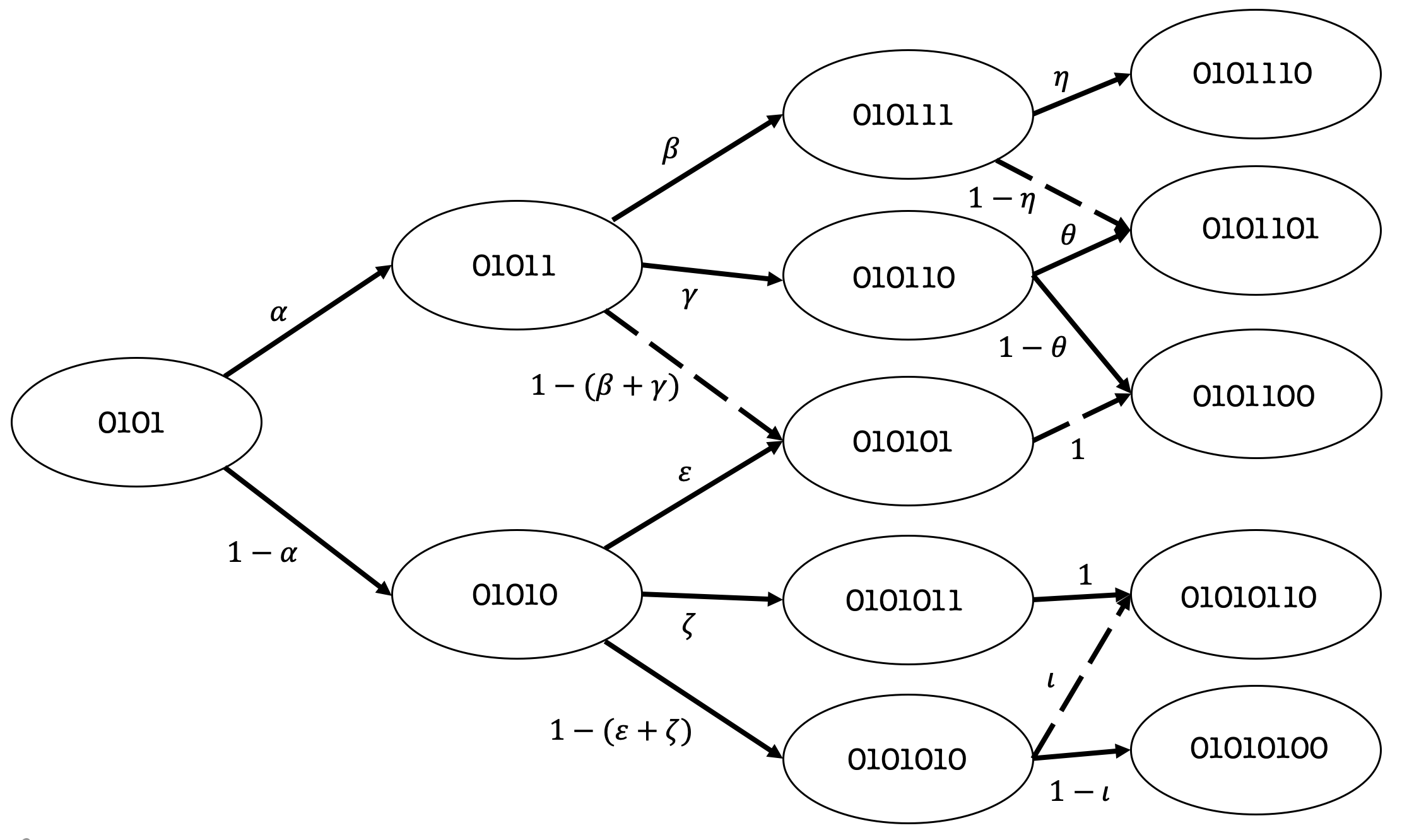
Figure 1: Directed graph showing several possible evolutions of the claims tape of an NDR machine for a binary alphabet. Dashed arrows denote both the deletion of bits on the claims tape and concatenation of additional bits onto the claims tape, whereas solid arrows denote only the concatenation of bits. Labels on arrows show transition probabilities from each claims list to the next, which are determined by the update distribution of the NDR machine.

The NDR machine starts with the questions and claims tapes blank. Then the NDR machine iterates a sequence of three steps. In the first step, it adds new questions to $Q$. In the second step the NDR machine “tries” to determine the valences of the questions in $Q$. In the third step, if the valence $v$ of one or more questions $q$ has been found, then the pair $(q,v)$ is added to the end of $C$, and $q$ is removed from $Q$. We also allow the possibility that some claims in $C$ are removed in this third step. The NDR machine iterates this sequence of three steps forever, i.e., it never halts. In this way the NDR machine randomly produces sequences of claims lists. We write the (random) claims list produced by an NDR machine after $k$ iterations as $C^{k}$, generated by a distribution $P^{k}$. (Note that $P^{k}(C)$ can be nonzero even if $|C|\neq k$, i.e., if the number of claims in $C$ differs from $k$.)

As an illustration, for any NDR machine that accurately models the real community of practicing mathematicians, the precise sequence of questions in the current claims list $C$ must have been generated in a somewhat random manner, reflecting randomness in which questions the community of mathematicians happened to consider first. The NDR machine models that randomness in the update distribution of the underlying PTM. In addition, in that NDR machine it is extremely improbable that a claim on the claims tape ever gets removed.

There are several restrictions on NDR machines which are natural to impose in certain circumstances, especially when using NDR machines to model the community of human mathematicians. In particular, we say that a claims list $C$ is non-repeating if it does not contain two claims that have the same question, otherwise it is repeating. We say that an NDR machine is non-repeating if it produces non-repeating claims lists with probability $1$. As an example, if the NDR machine of the community of mathematicians is non-repeating, then there might be hidden contradictions lurking in the set of all claims currently accepted by mathematicians, but there are not any explicit contradictions.

For each counting number $n$, let $\mathcal{C}_{n}$ be the set of all sequences of $n$ claims. For any current $C$ and any $n\leq|C|$, define $C(n)$ to be the sequence of the first $n$ claims in $C$. We say that a finite claims list $C$ is mistake-free if for every claim $(q,v)\in C$, $v$ is either $t,a,n,u$, depending on whether the question $q$ is $t$, $a,n$ or $u$, respectively. In other words, a claims list is mistake-free if every claim $(q,v)$ in that list, if $q=(\mathcal{S},\varphi)$, then $v$ is the syntactic valence assigned to $\varphi$ by $\mathcal{S}$. As an example, most (all?) current mathematicians view the “currently accepted body of mathematics” as a mistake-free claims list. (However, even if it so happened that that current claims list actually were mistake-free, we do not assume that humans can determine that fact; in fact, we presume that humans cannot make that determination in many instances.) We say that an NDR machine is mistake-free if for all finite $n$, the probability is $1$ that any claims list $C$ produced by the NDR machine will be mistake-free.

We want to analyze the stochastic properties of the claims list, in the limit that the mathematical reasoner has been running for very many iterations. To do that, we require that for any $n$, the probability distribution of sequences of claims $C^{k}(n)\in\mathcal{C}_{n}$ at the beginning of the claims list $C$ that has been produced by the NDR machine at its $k$’th iteration after starting from its initial state converges in probability in the limit of $k\rightarrow\infty$. We also require that the set of all repeating claims lists has probability $0$ under that limiting distribution. (Note though that we do not forbid repeating claims lists for finite $k$.) We further require that for all $n>0$, the infinite $k$ limit of the distribution over $C^{k}(n)$ is given by marginalizing the last (most recent) claim in the infinite $k$ limit of the distribution over $C^{k}({n+1})$. We write those limiting distributions as $P^{\infty}(C(n))$, one such distribution for each $n$.

For each $n$, the distribution $P^{\infty}(C(n))$ over all $n$-element claim sequences defines a probability distribution over all (unordered) claims sets $c=\{c_{i}\}$ containing $m\leq n$ claims:

$$P^{\infty}_{n}(c):=\sum_{C(n):\forall i,c_{i}\in C(n)}P^{\infty}(C(n))$$ (1)

(where $c_{i}\in C(n)$ means that claim $c_{i}$ occurs as one of the claims in the sequence $C(n)$). Under the assumptions of this essay, the $n\rightarrow\infty$ limit of this distribution over claims sets of size $m\leq n$ specifies an associated distribution over all finite claims sets, i.e., $\lim_{n\rightarrow\infty}P^{\infty}_{n}(c)$ is well-defined for any fixed, finite claims set $c$. We refer to this limiting distribution as the claims distribution of the underlying NDR machine, and write it as ${\overline{P}}(c)$. Intuitively, the claims distribution is the probability distribution over all possible bodies of mathematics that could end up being produced if current mathematicians kept working forever. We say that a claims list (resp., claims set) is maximal if it has nonzero probability under $P^{\infty}$ (resp., $\overline{P}$), and if it is not properly contained in a larger claims list (resp., claims set) that has nonzero probability.

Due to our assumption that there is zero probability of a repeating claims list under the claims distribution, the conditional distribution

$${\overline{P}}(v\;|\;q) :=\dfrac{{\overline{P}}((q,v))}{{\overline{P}}(q)}$$ (2)

$$=\dfrac{\lim_{n\rightarrow\infty}\sum_{C(n):(q,v)\in C(n)}P^{\infty}(C(n))}{\lim_{n\rightarrow\infty}\sum_{v^{\prime}}\sum_{C(n):(q,v^{\prime})\in C(n)}P^{\infty}(C(n))}$$ (3)

is well-defined for all $q$ that have nonzero probability of being in a claims set generated under the claims distribution. We refer to this conditional distribution ${\overline{P}}(v\;|\;q)$ as the answer distribution of the NDR machine. We will sometimes abuse terminology and use the same expression, “answer distribution”, even if we are implicitly considering ${\overline{P}}(v\;|\;q)$ restricted to a proper subset of the questions $q$ that can be produced by the NDR machine. As shorthand we will sometimes write answer distributions as ${{\cal{A}}}$.

A mistake-free answer distribution is one that can be produced by some mistake-free NDR machine. In general, there are an infinite number of NDR machines that all result in the same answer distribution ${\cal{A}}$. However, all NDR machines that result in a mistake-free answer distribution must themselves be mistake-free. For any claims list $C$ and question $q$ such that ${\overline{P}}(q,C)\neq 0$, we define

$${\overline{P}}(v\;|\;q,C) :=\dfrac{{\overline{P}}((q,v),C)}{{\overline{P}}(q,C)}$$ (4)

$$:=\dfrac{\lim_{n\rightarrow\infty}\sum_{C(n):(q,v)\cup C\in C(n)}P^{\infty}(C(n))}{\lim_{n\rightarrow\infty}\sum_{C(n),v^{\prime}:(q,v^{\prime})\cup C\in C(n)}P^{\infty}(C(n))}$$ (5)

and refer to this as a generalized answer distribution. (In the special case that $C$ is empty, the generalized answer distribution reduces to the answer distribution defined in (3).)

Claims distributions and (generalized) answer distributions are both defined in terms of the stochastic process that begins with the PTM’s question and claims tapes in their initial, blank states. We make analogous definitions conditioned on the PTM having run long enough to have produced a particular claims list $C$ at some iteration. (This will allow us to analyze the far-future distribution of claims of the actual current community of human mathematicians, conditioned on the actual claims list $C$ that that community has currently produced.)

Paralleling the definitions above, choose any pair $n_{1},n_{2}>n_{1}$ and any $C_{n_{1}}\in\mathcal{C}_{n_{1}}$ such that there is nonzero probability that the NDR machine will produce a sequence of claims lists one of which is $C_{n_{1}}$. We add the requirement that the probability distribution of sequences of claims $C^{k}(n_{2})\in\mathcal{C}_{n_{2}}$ at the beginning of the claims list $C$ that has been produced by the NDR machine at its $k$’th iteration after starting from its initial state, conditioned on its having had the claims list $C_{n_{1}}$ on its claims tape at some iteration $<k$, converges in probability in the limit of $k\rightarrow\infty$. With abuse of notation, we write that probability distribution as $P^{\infty}_{C_{n_{1}}}(C(n_{2}))$, and require that $P^{\infty}_{C_{n_{1}}}(C(n_{2}))$ is given by marginalizing out the last claim in $P^{\infty}_{C_{n_{1}}}(C(n_{2}+1))$. This distribution defines a probability distribution over all (unordered) claims sets $c=\{c_{i}:i=1,\ldots,m\}$ containing $m\leq n_{2}$ claims:

$$P^{\infty}_{C_{n_{1}};n_{2}}(c) :=\sum_{C(n_{2}):\forall i,c_{i}\in C(n_{2})}P^{\infty}_{C_{n_{1}}}(C(n_{2}))$$ (6)

We assume that $\lim_{n_{2}\rightarrow\infty}P^{\infty}_{C_{n_{1}};n_{2}}(c)$ is well-defined for any finite claims set $c$ (for all $C_{n-1}$ that are produced by the NDR machine with nonzero probability). We refer to this as a list-conditioned claims distribution, for conditioning claims list $C_{n_{1}}$, and write it as ${\overline{P}}_{C_{n_{1}}}(c)$. It defines an associated list-conditioned answer distribution, which we write as ${\cal{A}}_{C_{n_{1}}}(v\;|\;q)={\overline{P}}_{C_{n_{1}}}(v\;|\;q)$. We define the list-conditioned generalized answer distribution analogously. Intuitively, these are simply the distributions over bodies of mathematics that might be produced by the far-future community of mathematicians, conditioned on their having produced the claims list $C_{n_{1}}$ sometime in their past, while they were still young.

Note that the generalized answer distribution ${\overline{P}}(v\;|\;q,c)$ is defined in terms of a claims set $c$ which might have probability zero of being a contiguous sequence of claims, i.e., a claims list. In contrast, ${\overline{P}}_{C_{n_{1}}}(v\;|\;q)$ is defined in terms of a contiguous claims list $C_{n_{1}}$. Moreover, the claims in $C_{n_{1}}$ might have zero probability under the claims distribution, e.g., if the NDR machine removes them from the claims tape during the iterations after it first put them all onto the claims tape. Finally, note that both ${\overline{P}}(v\;|\;q,\{c\})$ and ${\overline{P}}_{C_{n_{1}}}(v\;|\;q)$ are limiting distributions, of the final conclusions of the far-future community of mathematicians. Both of these differ from the probability that as the NDR machine governing the current community of mathematicians evolves, starting from a current claims list and with a current open question $q$, it generates the answer $v$ for that question. (That answer might get overturned by the far-future community of mathematicians.)

4 Connections to Actual Mathematical Practice

In this section we show how NDR machines can be used to quantify and investigate some of the specific features of the behavior of human mathematicians (see also Viteri and DeDeo (2020)). Most of the analysis in this section holds even if we restrict attention to NDR machines whose answer distribution ${\cal{A}}$ is a probabilistic mixture of single-valued functions from $q\rightarrow v$. Intuitively, such NDR machines model scenarios where each question $({\mathcal{S}},\varphi)$ is mapped to a unique valence, but we are uncertain what that map from questions to valences is.

4.1 Generating New Research Questions

Given our supposition that the community of practicing mathematicians can be modeled as an NDR machine, what is the precise stochastic process that that NDR machine uses in each iteration, in the step where it adds new questions to $Q$. Phrased differently, what are the goals that guide how the community of mathematicians decides which open questions to investigate at any given moment?

This is obviously an extremely complicated issue, ultimately involving elements of sociology and human psychology. Nonetheless, it is possible to make some high-level comments. First, most obviously, one goal of human mathematicians is that there be high probability that they generate questions whose valence is either $t,a$ or $u$. Human mathematicians don’t want to “waste their time” considering questions $({\mathcal{S}},\varphi)$ where it turns out that $\varphi$ is not a WFF under ${\mathcal{S}}$. So we would expect there to be low probability that any such question is added to $Q$. Another goal is that mathematicians prefer to consider questions whose answer would be a “breakthrough”, leading to many fruitful “insights”. One way to formalize this second goal is that human mathematicians want to add questions $q$ to $Q$ such that, if they were able to answer $q$ (i.e., if they could determine the valence $v$ of $q$), then after they did so, and $C$ was augmented with that question-answer pair, the NDR machine would rapidly produce answers to many of the other open questions $q\in Q$.

4.2 Bayesian models of heuristics of human mathematicians – general considerations

Human mathematicians seem to act somewhat like Bayesian learners; as mathematicians learn more by investigating open mathematical questions — as their data set of mathematical conclusions grows larger — they update their probability distributions over those open questions. For example, modern computer scientists assign a greater probability to the claim $\mathsf{NP}\neq\mathsf{P}$ than did computer scientists of several decades ago. In the remainder of this section we show how to model this behavior in terms of NDR machines, and thereby gain new perspectives on some of the heuristic rules that seem to govern the reasoning of the human mathematical community

First, note that the subjective relative beliefs of the current community of mathematicians do not arise in the analysis up to this point. All probability distributions considered above concern what answers mathematicians are in fact likely to make, as the physical universe containing them evolves, not the answers that mathematicians happen to currently believe. Rather than introduce extra notation to explicitly model the current beliefs of mathematicians, for simplicity we suppose that the subjective relative beliefs of the current community of mathematicians, of what the answer is to all questions in the current questions tape, matches the actual answer distribution of the far-future community of mathematicians. As an example, under this supposition, if $C$ is the current claims list of the community of mathematicians and $\phi$ is the WFF, “$\mathsf{NP}\neq\mathsf{P}$” phrased in some particular formal system ${\mathcal{S}}$, then the current relative beliefs of the community of mathematicians concerning whether $\mathsf{NP}\neq\mathsf{P}$ just equals ${\overline{P}}(v=t\;|\;\phi,{\mathcal{S}})$.

4.3 A Bayesian Justification of Abduction in Mathematical Reasoning

Adopting this perspective, it is easy to show that the heuristic technique of “abductive reasoning” commonly used by human mathematicians is Bayes rational. To begin, let $q=({\mathcal{S}},\varphi),q^{\prime}=({\mathcal{S}},\varphi^{\prime})$ be two distinct open questions which share the same formal system ${\mathcal{S}}$ and are both contained in the current set of open questions of the community of mathematicians, $Q$, and so neither of which are contained in the current claims list of the community of mathematicians, $C$. Suppose as well that both $q$ and $q^{\prime}$ occur in ${\overline{P}}_{C}$ with probability $1$, i.e., the far-future community of mathematicians definitely has answers to both questions. Suppose as well that if $q^{\prime}$ were a theorem under ${\mathcal{S}}$, that would make it more likely that $q$ was also a theorem, i.e., suppose that

$${\overline{P}}_{C}\left(v=t\;|\;q,(q^{\prime},t)\right)>{\overline{P}}_{C}\left(v=t\;|\;q\right)$$ (7)

i.e.,

$$\dfrac{{\overline{P}}_{C}\left((q,t),(q^{\prime},t)\right)}{{\overline{P}}_{C}\left(q,(q^{\prime},t)\right)} >\dfrac{{\overline{P}}_{C}\left((q,t\right))}{{\overline{P}}_{C}(q)}$$ (8)

and so repeatedly using our assumption that both $q$ and $q^{\prime}$ occur with probability $1$,

$$\dfrac{{\overline{P}}_{C}\left((q,t),(q^{\prime},t)\right)}{{\overline{P}}_{C}\left((q^{\prime},t)\right)} >{\overline{P}}_{C}\left((q,t)\right)$$ (9)

$$\dfrac{{\overline{P}}_{C}\left((q,t),(q^{\prime},t)\right)}{{\overline{P}}_{C}\left((q,t)\right)} >{\overline{P}}_{C}\left((q^{\prime},t)\right)$$ (10)

$$\dfrac{{\overline{P}}_{C}\left((q,t),(q^{\prime},t)\right)}{{\overline{P}}_{C}\left(q^{\prime},(q,t)\right)} >\dfrac{{\overline{P}}_{C}\left((q^{\prime},t)\right)}{{\overline{P}}_{C}(q^{\prime})}$$ (11)

i.e.,

$${\overline{P}}_{C}\left(v=t\;|\;q^{\prime},(q,t)\right)>{\overline{P}}_{C}\left(v=t\;|\;q^{\prime}\right)$$ (12)

So no matter what the (list-conditioned, generalized) answer distribution of the far-future community of mathematicians ${\overline{P}}_{C}$ is, the probability that $q^{\prime}$ is true goes up if $q$ is true. Therefore under our supposition that the subjective beliefs of the current community of mathematicians are given by the claims distribution ${\overline{P}}_{C}$, not only is it Bayes-rational for them to increase their belief that $q^{\prime}$ is true if they find that $q$ is — modifying their beliefs this way will also lead them to mathematical truths (if we define “mathematical truths” by the claims distribution of the far-future community of mathematicians).

Stripped down, this inference pattern can be explained in two simple steps. First, suppose that mathematicians believe that some hypothesis $H$ would be more likely to be true if a different hypothesis $H^{\prime}$ were true. Then if they find out that $H$ actually is true, they must assign higher probability to $H^{\prime}$ also being true. This general pattern of reasoning, in which we adopt a greater degree of belief in one hypothesis because it would lend credence to some other hypothesis that we already believe to be true, is known as “abduction” (Peirce, 1960), and plays a prominent role in actual mathematical practice (Viteri and DeDeo, 2020). As we have just shown, it is exactly the kind of reasoning one would expect mathematicians to use if they were Bayesian reasoners making inferences about their own answer distribution ${\cal{A}}$.

4.4 A Bayesian Formulation of the Value of Multiple Proof Paths in Mathematical Reasoning

Real human mathematicians often have higher confidence that some question $q$ is a theorem if many independent paths of reasoning suggest that it is a theorem. To understand why this might be Bayes-rational, as before, let $C$ be the current claims list of the community of mathematicians and let $Q$ be the current list of open questions. Let $\{\{c\}_{1},\dots\{c\}_{n}\}$ be a set of sets of claims, none of which are in $C$. By Bayes’ theorem,

$${\overline{P}}_{C}\big{(}v=t\,|\,q,\{c\}_{1},\dots,\{c\}_{n}\big{)}=\frac{{\overline{P}}_{C}\big{(}\{c\}_{1},\dots,\{c\}_{n}\,|\,\big{(}q,t\big{)}\big{)}{\overline{P}}_{C}\big{(}v=t\,|\,q\big{)}}{{\overline{P}}_{C}\big{(}\{c\}_{1},\dots,\{c\}_{n}\,|\,q\big{)}}$$ (13)

Expanding ${\overline{P}}_{C}\big{(}\{c\}_{1},\dots,\{c\}_{n}\,|\,q\big{)}$ in the denominator gives

$${\overline{P}}_{C}\big{(}v=t\,|\,q,\{c\}_{1},\dots,\{c\}_{n}\big{)}$$

$$\qquad=\frac{{\overline{P}}_{C}\big{(}\{c\}_{1},\dots,\{c\}_{n}\,|\,(q,v=t)\big{)}{\overline{P}}_{C}\big{(}v=t\,|\,q\big{)}}{{\overline{P}}_{C}\big{(}\{c\}_{1},\dots,\{c\}_{n}\,|\,(q,v\neq t)\big{)}{\overline{P}}_{C}\big{(}v\neq t\,|\,q\big{)}\;+\;{\overline{P}}_{C}\big{(}\{c\}_{1},\dots,\{c\}_{n}\,|\,(q,v=t)\big{)}{\overline{P}}_{C}\big{(}v=t\,|\,q\big{)}}$$ (14)

Next, for all $1<i\leq n$ define

$$\alpha_{i} :=\dfrac{{\overline{P}}_{C}\big{(}\{c\}_{1},\dots,\{c\}_{i}\,|\,(q,v=t)\big{)}}{{\overline{P}}_{C}\big{(}\{c\}_{1},\dots,\{c\}_{i-1}\,|\,(q,v=t)\big{)}}$$ (15)

$$={\overline{P}}_{C}\big{(}\{c\}_{i}\,|\,\{c\}_{1},\dots,\{c\}_{i-1},(q,v=t)\big{)}$$ (16)

$$\beta_{i} :=\dfrac{{\overline{P}}_{C}\big{(}\{c\}_{1},\dots,\{c\}_{i}\,|\,(q,v\neq t)\big{)}}{{\overline{P}}_{C}\big{(}\{c\}_{1},\dots,\{c\}_{i-1}\,|\,(q,v\neq t)\big{)}}$$ (17)

$$={\overline{P}}_{C}\big{(}\{c\}_{i}\,|\,\{c\}_{1},\dots,\{c\}_{i-1},(q,v\neq t)\big{)}$$ (18)

Note that due to Eqs. 16 and 18, we can write

$$\dfrac{\alpha_{i}}{\beta_{i}} =\dfrac{{\overline{P}}_{C}\left(v=t\,|\,q,\{c\}_{1},\ldots,\{c\}_{i-1}\right)}{{\overline{P}}_{C}\left(v\neq t\,|\,q,\{c\}_{1},\ldots,\{c\}_{i-1}\right)}$$ (19)

So $\alpha_{i}\geq\beta_{i}$ iff ${\overline{P}}_{C}\left(v=t\,|\,q,\{c\}_{1},\ldots,\{c\}_{i-1}\right)\geq 1/2$. We say that all $\{c\}_{i}$ in the set $\{\{c\}_{i}\}$ are proof paths if $\alpha_{i}\geq\beta_{i}$ for all $1<i\leq n$.

As an example, suppose that in fact for all $1<i\leq n$,

$${\overline{P}}_{C}\big{(}\{c\}_{i}\,|\,\{c\}_{1},\dots,\{c\}_{i-1},(q,v=t)\big{)} ={\overline{P}}_{C}\big{(}\{c\}_{i}\,|\,(q,v=t)\big{)}$$ (20)

$${\overline{P}}_{C}\big{(}\{c\}_{i}\,|\,\{c\}_{1},\dots,\{c\}_{i-1},(q,v\neq t)\big{)} ={\overline{P}}_{C}\big{(}\{c\}_{i}\,|\,(q,v\neq t)\big{)}$$ (21)

In this case, $\{c\}_{i}$ is a proof path so long as the probability that the far-future community of mathematicians concludes the claims in $\{c\}_{i}$ are all true is larger if they also conclude that $q$ is true than it is if they conclude that $q$ is not true. Intuitively, if the claims in $\{c\}_{i}$ are more likely to lead to the conclusion that $q$ is true (i.e., are more likely to be associated with the claim $(q,t)$) than to the conclusion that $q$ is false, then $\{c\}_{i}$ is a proofs path.

Plugging Eqs. 15 and 18 into Eq. 14 gives

$${\overline{P}}_{C}\big{(}v=t\,|\,q,\{c\}_{1},\dots,\{c\}_{n}\big{)}$$

$$\qquad=\dfrac{\alpha_{n}}{\beta_{n}}\frac{{\overline{P}}_{C}\big{(}\{c\}_{1},\dots,\{c\}_{n-1}\,|\,(q,v=t)\big{)}{\overline{P}}_{C}\big{(}v=t\,|\,q\big{)}}{{\overline{P}}_{C}\big{(}\{c\}_{1},\dots,\{c\}_{n-1}\,|\,(q,v\neq t)\big{)}{\overline{P}}_{C}\big{(}v\neq t\,|\,q\big{)}\;+\;\dfrac{\alpha_{n}}{\beta_{n}}{\overline{P}}_{C}\big{(}\{c\}_{1},\dots,\{c\}_{n-1}\,|\,(q,v=t)\big{)}{\overline{P}}_{C}\big{(}v=t\,|\,q\big{)}}$$ (22)

If we evaluate Eq. 14 for $n-1$ rather than $n$ and then rearrange it to evaluate the numerator in Eq. 22, we get

$$\dfrac{{\overline{P}}_{C}\big{(}v=t\,|\,q,\{c\}_{1},\dots,\{c\}_{n}\big{)}}{{\overline{P}}_{C}\big{(}v=t\,|\,q,\{c\}_{1},\dots,\{c\}_{n-1}\big{)}}$$

$$\;\;=\dfrac{\alpha_{n}}{\beta_{n}}\frac{{\overline{P}}_{C}\big{(}\{c\}_{1},\dots,\{c\}_{n-1}\,|\,(q,v\neq t)\big{)}{\overline{P}}_{C}\big{(}v\neq t\,|\,q\big{)}\;+\;{\overline{P}}_{C}\big{(}\{c\}_{1},\dots,\{c\}_{n-1}\,|\,(q,v=t)\big{)}{\overline{P}}_{C}\big{(}v=t\,|\,q\big{)}}{{\overline{P}}_{C}\big{(}\{c\}_{1},\dots,\{c\}_{n-1}\,|\,(q,v\neq t)\big{)}{\overline{P}}_{C}\big{(}v\neq t\,|\,q\big{)}\;+\;\dfrac{\alpha_{n}}{\beta_{n}}{\overline{P}}_{C}\big{(}\{c\}_{1},\dots,\{c\}_{n-1}\,|\,(q,v=t)\big{)}{\overline{P}}_{C}\big{(}v=t\,|\,q\big{)}}$$ (23)

$$\;\;:=\epsilon_{n}$$ (24)

Iterating gives

$${\overline{P}}_{C}\big{(}v=t\,|\,q,\{c\}_{1},\dots,\{c\}_{n}\big{)} ={\overline{P}}_{C}\big{(}v=t\,|\,q,\{c\}_{1}\big{)}\prod_{i=2}^{n}\epsilon_{i}$$ (25)

Next, note that $\alpha_{i}\geq\beta_{i}$ implies that $\epsilon_{i}\geq 1$. So Eq. 25 tells us that if each $\{c\}_{i}$ is a proof path, i.e., $\epsilon_{i}>1$ for all $i>1$, then the posterior probability of $q$ being true keeps growing as more of the $n$ proof paths are added to the set of claims accepted by the far-future community of mathematicians.

This formally establishes the claim in the introduction, that the NDR machine model of human mathematicians lends formal justification to the idea that, everything else being equal, a mathematical claim should be believed more if there are multiple distinct lines of reasoning supporting that claim.

5 Measures over Multiverses

The mathematical universe hypothesis (MUH) argues that our physical universe is just one particular formal system, namely, the one that expresses the laws of physics of our universe (Schmidhuber, 1997, Tegmark, 1998, Hut et al., 2006, Tegmark, 2008, 2009, 2014). Similar ideas are advocated by Barrow (1991, 2011), who uses the phrase “pi in the sky” to describe this view. Somewhat more precisely, the MUH is the hypothesis that our physical world is isomorphic to a formal system. A key advantage of the MUH is that it allows for a straightforward explanation of why it is the case that, to use Wigner’s (1960) phrase, mathematics is “unreasonably effective” in describing the natural world. If the natural world is, by definition, isometric to mathematical structures, then the isometry between nature and mathematics is no mystery; rather, it is a tautology. While the MUH is accepted (implicitly or otherwise) by many theoretical physicists working in cosmology, some disagree with various aspects of it; for an overview of the controversy, see Hut et al. (2006).

Here, we adapt the MUH into the framework of NDR machines. Suppose we have a claims distribution that is a delta function about some formal system ${\mathcal{S}}$, in the sense that the probability of any claim whose question does not specify the formal system ${\mathcal{S}}$ is zero under that distribution. Similarly, suppose that any string $\varphi$ which is a WFF under ${\mathcal{S}}$ has nonzero probability under the claims distribution. (The reason for this second condition is to ensure that the answer distribution, ${\cal{A}}(v\;|\;({\mathcal{S}},\varphi))={\overline{P}}(v\;|\;({\mathcal{S}},\varphi))$, is well-defined for any $\varphi$ which is a WFF under ${\mathcal{S}}$.) We refer to the associated pair $({\mathcal{S}},{\cal{A}})$ of any such claims distribution as an NDR world. Similarly, we define an NDR world instance of an NDR machine as any associated pair $({\mathcal{S}},c)$ where $c$ is a maximal claims set of that NDR machine.

Intuitively, an NDR world is the combination of a formal system and the set of answers that some NDR machine would provide to questions formulated in terms of that formal system, without specifying a distribution over such questions. An NDR world instance is a sample of that NDR machine. (It is not clear what a distribution over questions would amount to in a physical universe, which is why we exclude such distributions from both definitions.) A mistake-free NDR world is any NDR world with a mistake-free answer distribution, and similarly for an NDR world instance. Note that while a mistake-free NDR world can only produce an NDR world instance that is mistake-free, mistake-free NDR world instances can be produced by NDR worlds that are not mistake free.

Rephrased in terms of our framework, previous versions of the MUH hold that our physical universe is a mistake-free NDR world. That is, the physical universe is isomorphic to a particular formal system $\mathcal{S}$ which in turn assigns, with certainty, a specific syntactic valence to each possible string in the alphabet of $\mathcal{S}$. Our approach can be used to generalize this in two ways. First, it allows for the possibility that the physical world is isomorphic to an NDR world that is not mistake-free. Second, it allows for the possibility that the physical world is isomorphic to an NDR world instance that is not mistake-free. In such a world, some strings would have their syntactic valence not because of the perfect application of the rules of some formal system, but rather because of the stochastic application of those very rules.

Thus, our augmented version of the MUH allows for the possibility that mathematical reality is fundamentally stochastic. So in particular, the mathematical reality governing our physical universe may be stochastic. This is similar to the fact that physical reality is fundamentally stochastic (or at least can be interpreted that way, under some interpretations of quantum mechanics).

An idea closely related to the MUH as just defined is the mathematical multiverse hypothesis (MMH). The MMH says that some non-singleton subset of formal systems is such that there is a physical universe that is isomorphic to each element of that subset. Each of these possible physical universes is taken to be perfectly real, in the sense that the formal system to which that universe is isomorphic is not just the fictitious invention of a mathematician, but rather a description of a physical universe. In this view, the world that we happen to live in is unique not because it is uniquely real, but because it is our actual world. Following Lewis (1973), defenders of the MMH understand claims about ‘the actual universe’ as indexical expressions, i.e. expressions whose meaning can shift depending on contingent properties of their speaker (pp. 85-86).

A central concern of people working on the MMH (e.g. Schmidhuber 1997 and Tegmark 2014) is how to specify a probability measure over the set of all universes, which we will refer to as an MMH measure. Implicitly, the concern is not merely to specify the subjectivist, degree of belief of us humans about what the laws of physics are in our particular universe. (After all, the MMH measures considered in the literature assign nonzero prior probability to formal systems that are radically different from the laws of our universe, supposing such formal systems are just as “real” as the one that governs our universe.) Rather the MMH measure is typically treated as more akin to the objective probability probability distributions that arise in quantum mechanics, as quantifying something about reality, not just about human ignorance.

In existing approaches to MMH measures, it is assumed that any physical reality is completely described by a set of recursive rules that assign, with certainty, a particular syntactic valence to any string. As mentioned above, this amounts to the assumption that all physical universes are mistake-free NDR worlds. So the conventional conception of an MMH measure is a distribution over mistake-free NDR worlds, i.e., over NDR world instances that are mistake-free. A natural extension, of course, is to have the MMH measure be a distribution over all NDR world instances, not just those that are mistake-free. A variant would be to have the MMH measure be a distribution over all NDR worlds, not just those that are mistake-free. Another possibility, in some ways more elegant than these two, would be to use a single NDR machine to define a measure over NDR world instances, and identify that measure as the MMH measure.

6 Future research directions

There are many possible directions for future research. For example, in general, for any $q$ produced with nonzero probability, the PTM underlying the NDR machine of the community of mathematicians will cause the answer distribution ${\overline{P}}(v\,|\,q)$ not to be a delta function about one particular valence $v$. This is also true for distributions concerning the current community of mathematicians: letting $((q,v),C)$ be the current sequence of claims actually accepted by that community, and supposing it was produced by $k$ iterations of the underlying PTM, $P^{k}(v\,|\,q,C)$ need not equal $1$. In other words, if we were to re-sample the stochastic process that resulted in the current claims list of the community of mathematicians, then even conditioning on the question $q$ being on that claims list, and even conditioning on the other, earlier claims in that list, $C$, there may be nonzero probability of producing a different answer to $q$ from the one actually accepted by the current community of mathematicians.

This raises the obvious question of how $P^{k}(v\,|\,q,C)$ would change if we modified the update distribution of the PTM underlying that NDR machine. In particular, there are many famous results in the foundations of mathematics that caused dismay when they were discovered, starting with the problems that were found in naive set theory, through Godel’s incompleteness theorems on to the proof that both the continuum hypothesis and its negation are consistent with the axioms of modern set theory. A common feature of these mathematical results is that they restrict mathematics itself, in some sense, and so have implications for the answers to many questions. Note though that all of those results were derived using deductive reasoning, expressible in terms of a formal system. So they can be formulated as claims by an NDR machine. This raises the question of how robust those results are with respect to the noise level in that NDR machine. More precisely, if those results are formulated as claims of the NDR machine, and some extremely small extra stochasticity is introduced into the PTM underlying the NDR machine, do the probabilities of those results – the probability distribution over the valences associated with the questions – change radically? Can we show that the far-ranging results in mathematics that restrict its own capabilities are fragile with respect to errors in mathematical reasoning? Or conversely, can we show that they are unusually robust with respect to such errors?

As another example of possible future research, the field of epistemic logic is concerned with how to formally model what it means to “know” that a proposition is true. Most epistemic logic models require that knowledge be transitive, meaning that if one knows some proposition $A$, and knows that $A\Rightarrow B$, then one knows $B$ (Fagin et al., 2003, Aaronson, 2013). Such models are subject to an infamous problem known as logical omniscience: supposing only that one knows the axioms of standard number theory and Boolean algebra, by recursively applying transitivity it follows that one “knows” all theorems in number theory — which is clearly preposterous.

Note though that any such combination of standard number theory and Boolean algebra is a formal system. This suggests that we replace conventional epistemic logic with an NDR machine version of epistemic logic, where the laws of Boolean algebra are only stochastic rather than iron-clad. In particular, by doing that, the problem of logical omniscience may be resolved: it may be that for any non-zero level of noise in the NDR machine, and any $0<\epsilon<1$, there is some associated finite integer $n$ such that one knows no more than $n$ theorems of number theory with probability greater than $\epsilon$.

As another example of possible future work, the models of practicing mathematicians as NDR machines introduced in Section 4 are very similar to the kind of models that arise in active learning (Settles, 2009), a subfield of machine learning. Both kinds of model are concerned with an iterated process in which one takes a current data set $C$, consisting of pairs of inputs (resp., questions) and associated outputs (resp., valences); uses $C$ to suggest new inputs (resp., questions); evaluates the output (resp., valence) for that new input (resp., question); and adds the resulting pair to the data set $C$. This formal correspondence suggests that it may be fruitful to compare how modern mathematical research is conducted with the machine learning techniques that have been applied to active learning, etc.

In this regard, recall that the no free lunch theorems are a set of formal bounds on how well any machine learning algorithm or search algorithm can be guaranteed to perform if one does not make assumptions for the prior probability distribution of the underlying stochastic process (Wolpert, 1996, Wolpert and Macready, 1997). Similar bounds should apply to active learning. Given the formal correspondence between the model of mathematicians as NDR machines and active learning algorithms, this suggests that some version of the NFL theorems should be applicable to the entire enterprise of mathematics research. Such bounds would limit how strong any performance guarantees for modern mathematical research practices can be without making assumptions for the prior distribution over the possible answer distributions of the infinite-future community of mathematicians, ${\overline{P}}({\cal{A}})$.

7 Conclusion

Starting from the discovery of non-Euclidean geometry, mathematics has been greatly enriched whenever it has weakened its assumptions and expanded the range of formal possibilities that it considers. Following in that spirit of weakening assumptions, we introduced a way to formalize mathematics in a stochastic fashion, without the the assumption that mathematics itself is fully deterministic. We showed that this formalism justifies some common heuristics of actual mathematical practice. We also showed how it extends and clarifies some aspects of the multi-universe hypothesis.

Appendix A Probabilistic Turing Machines

Perhaps the most famous class of computational machines are Turing machines. One reason for their fame is that it seems one can model any computational machine that is constructable by humans as a Turing machine. A bit more formally, the Church-Turing thesis states that “a function on the natural numbers is computable by a human being following an algorithm, ignoring resource limitations, if and only if it is computable by a Turing machine.”

There are many different definitions of Turing machines (TMs) that are “computationally equivalent” to one another. For us, it will suffice to define a TM as a 7-tuple $(R,\Lambda,b,v,r^{\varnothing},r^{A},\rho)$ where:

1. $R$ is a finite set of computational states;

2. $\Lambda$ is a finite alphabet containing at least three symbols;

3. $b\in\Lambda$ is a special blank symbol;

4. $v\in{\mathbb{Z}}$ is a pointer;

5. $r^{\varnothing}\in R$ is the start state;

6. $r^{A}\in R$ is the halt state; and

7. $\rho:R\times{\mathbb{Z}}\times\Lambda^{\infty}\rightarrow R\times{\mathbb{Z}}\times\Lambda^{\infty}$ is the update function. It is required that for all triples $(r,v,T)$, that if we write $(r^{\prime},v^{\prime},T^{\prime})=\rho(r,v,T)$, then $v^{\prime}$ does not differ by more than $1$ from $v$, and the vector $T^{\prime}$ is identical to the vectors $T$ for all components with the possible exception of the component with index $v$;

We sometimes refer to $R$ as the states of the “head” of the TM, and refer to the third argument of $\rho$ as a tape, writing a value of the tape (i.e., of the semi-infinite string of elements of the alphabet) as $T$.

Any TM $(R,\Sigma,b,v,r^{\varnothing},r^{A},\rho)$ starts with $r=r^{\varnothing}$, the counter set to a specific initial value (e.g, $0$), and with $T$ consisting of a finite contiguous set of non-blank symbols, with all other symbols equal to $b$. The TM operates by iteratively applying $\rho$, until the computational state falls in $r^{A}$, at which time it stops, i.e., any ID with the head in the halt state is a fixed point of $\rho$.

If running a TM on a given initial state of the tape results in the TM eventually halting, the largest blank-delimited string that contains the position of the pointer when the TM halts is called the TM’s output. The initial state of $T$ (excluding the blanks) is sometimes called the associated input, or program. (However, the reader should be warned that the term “program” has been used by some physicists to mean specifically the shortest input to a TM that results in it computing a given output.) We also say that the TM computes an output from an input. In general, there will be inputs for which the TM never halts. The set of all those inputs to a TM that cause it to eventually halt is called its halting set.

The set of triples that are possible arguments to the update function of a given TM are sometimes called the set of instantaneous descriptions (IDs) of the TM. Note that as an alternative to the definition in (7) above, we could define the update function of any TM as a map over an associated space of IDs.

In one particularly popular variant of this definition of TMs the single tape is replaced by multiple tapes. Typically one of those tapes contains the input, one contains the TM’s output (if and) when the TM halts, and there are one or more intermediate “work tapes” that are in essence used as scratch pads. The advantage of using this more complicated variant of TMs is that it is often easier to prove theorems for such machines than for single-tape TMs. However, there is no difference in their computational power. More precisely, one can transform any single-tape TM into an equivalent multi-tape TM (i.e., one that computes the same partial function), as shown by Arora and Barak (2009).

A universal Turing machine (UTM), $M$, is one that can be used to emulate any other TM. More precisely, in terms of the single-tape variant of TMs, a UTM $M$ has the property that for any other TM $M^{\prime}$, there is an invertible map $f$ from the set of possible states of the tape of $M^{\prime}$ into the set of possible states of the tape of $M$, such that if we:

1. apply $f$ to an input string $\sigma^{\prime}$ of $M^{\prime}$ to fix an input string $\sigma$ of $M$;

2. run $M$ on $\sigma$ until it halts;

3. apply $f^{-1}$ to the resultant output of $M$;

then we get exactly the output computed by $M^{\prime}$ if it is run directly on $\sigma^{\prime}$.

An important theorem of computer science is that there exist universal TMs (UTMs). Intuitively, this just means that there exists programming languages which are “universal”, in that we can use them to implement any desired program in any other language, after appropriate translation of that program from that other language. The physical CT thesis considers UTMs, and we implicitly restrict attention to them as well.

Suppose we have two strings $s^{1}$ and $s^{2}$ where $s^{1}$ is a proper prefix of $s^{2}$. If we run the TM on $s^{1}$, it can detect when it gets to the end of its input, by noting that the following symbol on the tape is a blank. Therefore, it can behave differently after having reached the end of $s^{1}$ from how it behaves when it reaches the end of the first $\ell(s^{1})$ bits in $s^{2}$. As a result, it may be that both of those input strings are in its halting set, but result in different outputs. A prefix (free) TM is one in which this can never happen: there is no string in its halting set that is a proper prefix of another string in its halting set. For technical reasons, it is conventional in the physics literature to focus on prefix TMs, and we do so here.

The coin-flipping distribution of a prefix TM $M$ is the probability distribution over the strings in $M$’s halting set generated by IID “tossing a coin” to generate those strings, in a Bernoulli process, and then normalizing. So any string $\sigma$ in the halting set has probability $2^{-\;|\;\sigma\;|\;}/\Omega$ under the coin-flipping prior, where $\Omega$ is the normalization constant for the TM in question.

Finally, for our purposes, a Probabilistic Turing Machine (PTM) is a conventional TM as defined by conditions (1)-(7), except that the update function $\rho$ is generalized to be a conditional distribution. The conditional distribution is not arbitrary however. In particular, we typically require that there is zero probability that applying such an update conditional distribution violates condition (7). Depending on how we use a PTM to model NDR machines, we may introduce other requirements as well.

References

- Aaronson (2013) S. Aaronson. Why philosophers should care about computational complexity. In Computability: Turing, Gödel, Church, and Beyond, pages 261–327. MIT Press, 2013.
- Arora and Barak (2009) S. Arora and B. Barak. Computational complexity: a modern approach. Cambridge University Press, 2009.
- Barrow (1991) J. D. Barrow. Theories of everything: The quest for ultimate explanation. Clarendon Press Oxford, 1991.
- Barrow (2011) J. D. Barrow. Godel and physics. Kurt Gödel and the Foundations of Mathematics: Horizons of Truth, page 255, 2011.
- Carroll (2010) J. L. Carroll. A bayesian decision theoretical approach to supervised learning, selective sampling, and empirical function optimization. 2010.
- Fagin et al. (2003) R. Fagin, Y. Moses, J. Y. Halpern, and M. Y. Vardi. Reasoning about knowledge. MIT press, 2003.
- Gödel (1934) K. Gödel. On undecidable propositions of formal mathematics systems. Institute for Advanced Study, 1934.
- Grunwald and Vitányi (2004) P. Grunwald and P. Vitányi. Shannon information and kolmogorov complexity. arXiv preprint cs/0410002, 2004.
- Hilbert (1928) D. Hilbert. Die grundlagen der mathematik. In Die Grundlagen der Mathematik, pages 1–21. Springer, 1928.
- Hume (2012) D. Hume. A treatise of human nature. Courier Corporation, 2012. Book 1, Part 4, Section 1.
- Hut et al. (2006) P. Hut, M. Alford, and M. Tegmark. On math, matter and mind. Foundations of Physics, 36(6):765–794, 2006.
- Lewis (1973) D. Lewis. Counterfactuals. Oxford: Basil Blackwell, 1973.
- Peirce (1960) C. S. Peirce. Collected papers of charles sanders peirce, volume 2. Harvard University Press, 1960.
- Poincaré (1910) H. Poincaré. Mathematical creation. The Monist, pages 321–335, 1910.
- Schmidhuber (1997) J. Schmidhuber. A computer scientist’s view of life, the universe, and everything. In Foundations of computer science, pages 201–208. Springer, 1997.
- Settles (2009) B. Settles. Active learning literature survey. Technical report, University of Wisconsin-Madison Department of Computer Sciences, 2009.
- Tegmark (1998) M. Tegmark. Is “the theory of everything” merely the ultimate ensemble theory? Annals of Physics, 270(1):1–51, 1998.
- Tegmark (2008) M. Tegmark. The mathematical universe. Foundations of physics, 38(2):101–150, 2008.
- Tegmark (2009) M. Tegmark. The multiverse hierarchy. arXiv preprint arXiv:0905.1283, 2009.
- Tegmark (2014) M. Tegmark. Our mathematical universe: My quest for the ultimate nature of reality. Vintage, 2014.
- Viteri and DeDeo (2020) S. Viteri and S. DeDeo. Explosive proofs of mathematical truths. arXiv preprint arXiv:2004.00055, 2020.
- Wigner (1960) E. P. Wigner. The unreasonable effectiveness of mathematics in the natural sciences. 13:1–14, 1960.
- Wolpert (1996) D. H. Wolpert. The lack of a priori distinctions between learning algorithms. Neural computation, 8(7):1341–1390, 1996.
- Wolpert (2019) D. H. Wolpert. The stochastic thermodynamics of computation. Journal of Physics A: Mathematical and Theoretical, 52(19):193001, 2019.
- Wolpert and Macready (1997) D. H. Wolpert and W. G. Macready. No free lunch theorems for optimization. IEEE Transactions on Evolutionary Computation, 1(1):67–82, 1997.