A Trajectory-Based Approach to Discrete-Time Flatness

Abstract

For discrete-time systems, flatness is usually defined by replacing the time-derivatives of the well-known continuous-time definition by forward-shifts. With this definition, the class of flat systems corresponds exactly to the class of systems which can be linearized by a discrete-time endogenous dynamic feedback as it is proposed in the literature. Recently, verifiable necessary and sufficient differential-geometric conditions for this property have been derived. In the present contribution, we make an attempt to take into account also backward-shifts. This extended approach is motivated by the one-to-one correspondence of solutions of flat systems to solutions of a trivial system as it is known from the continuous-time case. If we transfer this idea to the discrete-time case, this leads to an approach which also allows backward-shifts. To distinguish the classical definition with forward-shifts and the approach of the present paper, we refer to the former as forward-flatness. We show that flat systems (in the extended sense with backward-shifts) still share many beneficial properties of forward-flat systems. In particular, they still are reachable/controllable, allow a straightforward planning of trajectories and can be linearized by a certain subclass of dynamic feedbacks.

I Introduction

In the 1990s, the concept of flatness has been introduced by Fliess, Lévine, Martin and Rouchon for nonlinear continuous-time systems (see e.g. [1] and [2]). Flat continuous-time systems have the characteristic feature that all system variables can be parameterized by a flat output and its time derivatives. This leads to a one-to-one correspondence of solutions of a flat system to solutions of a trivial system with the same number of inputs. Flat systems form an extension of the class of static feedback linearizable systems and can be linearized by an endogenous dynamic feedback. Their popularity stems from the fact that many physical systems possess the property of flatness and that the knowledge of a flat output allows an elegant solution to motion planning problems and design of tracking controllers.

For nonlinear discrete-time systems, flatness is usually defined by replacing the time-derivatives of the well-known continuous-time definition by forward-shifts. More precisely, the flat output is a function of the state variables, input variables, and forward-shifts of the input variables. Conversely, the state- and input variables can be expressed as functions of the flat output and its forward-shifts. This point of view has been adopted in [3], [4] and [5]. With this definition, the class of flat systems corresponds exactly to the class of systems which can be linearized by a discrete-time endogenous dynamic feedback as it is proposed e.g. in [6]. Recently, verifiable necessary and sufficient differential-geometric conditions have been derived in [7] and [8]. Furthermore, in [9] it has been shown that in the two-input case even a transformation into a certain normal form is always possible.

In this contribution, we focus solely on the one-to-one correspondence of solutions of flat systems to solutions of a trivial system (arbitrary trajectories that need not satisfy any equation) with the same number of inputs, as it is known from the continuous-time case. For discrete-time systems, this would mean that the flat output may depend both on forward- and backward-shifts of the system variables. Conversely, the state- and input variables could be expressed as functions of both forward- and backward-shifts of the flat output. To distinguish the usual definition of [3], [4] and [5] with forward-shifts from the alternative approach of the present paper, we refer to the former as forward-flatness. A special case of this alternative definition has already been suggested in [10], where the flat output may depend also on backward-shifts of the input variables but not on backward-shifts of the state variables. To justify our alternative approach, we show that flat systems (in the extended sense with backward-shifts) still share many beneficial properties of forward-flat systems. In particular, we show that they still are reachable (and hence controllable) and allow a straightforward planning of trajectories to connect arbitrary points of the state space. Furthermore, we show that they can be linearized by a dynamic feedback which shares the beneficial properties of the class of continuous-time endogenous feedback. With respect to the classical dynamic feedback linearization problem, the following inclusions hold: (static feedback linearizable systems) $\subset$ (forward-flat systems) $\subset$ (flat systems) $\subset$ (dynamic feedback linearizable systems). We show that for single-input and linear systems the properties of flatness, forward-flatness and static feedback linearizability are equivalent, and present an example which shows that the class of forward-flat systems is a strict subset of the class of flat systems in the extended sense.

The paper is organized as follows: In Section II we introduce the extended concept of flatness with both forward- and backward-shifts and illustrate it by an example. Subsequently, we discuss the special case of single-input systems. In Section III we first demonstrate the planning of trajectories, prove the reachability of flat systems and apply the concept to the sampled-data model of an induction motor. Second, we show that flat systems can be linearized by a particular subclass of dynamic feedbacks.

II Discrete-Time Flatness with Forward- and Backward-Shifts

Throughout this contribution, we consider time-invariant discrete-time nonlinear systems in state representation of the form

$$x^{i,+}=f^{i}(x,u)\,,\quad i=1,\dots,n$$ (1)

with $\dim(x)=n$, $\dim(u)=m$ and smooth functions $f^{i}(x,u)$. We assume that the systems meet the submersivity condition, i.e. that the Jacobian-matrix of $f$ with respect to $(x,u)$ meets

$$\operatorname{rank}(\partial_{(x,u)}f)=n\,.$$ (2)

This condition is necessary for reachability and consequently also for flatness. However, we want to emphasize that we do not require $\operatorname{rank}(\partial_{x}f)=n$. As mentioned in [6], this property is always met by systems which stem from the exact or approximate discretization of continuous-time systems. However, we want to consider discrete-time systems in general, no matter whether they stem from a discretization or not.

II-A Equivalence of Solutions

To motivate our trajectory-based approach, we want to recall that a continuous-time system $\dot{x}=f(x,u)$ is flat if there exists a one-to-one correspondence between its solutions $(x(t),u(t))$ and solutions $y(t)$ of a trivial system (sufficiently smooth but otherwise arbitrary trajectories) with the same number of inputs (see e.g. [2]).

In the following, we attempt to define flatness for discrete-time systems in exactly the same way. Within this paper, we call a discrete-time system (1) flat if there exists a one-to-one correspondence between its solutions $(x(k),u(k))$ and solutions $y(k)$ of a trivial system (arbitrary trajectories that need not satisfy any difference equation) with the same number of inputs.

$$\begin{array}[]{ccc}x^{+}=f(x,u)&&\begin{aligned} \text{trivial system}\end{aligned}\\ \downarrow&&\downarrow\\ (x(k),u(k))&\overset{\text{one-to-one}}{\Longleftrightarrow}&(y(k))\end{array}$$

By one-to-one correspondence, we mean that the values of $x(k)$ and $u(k)$ at some fixed time step $k$ may depend on an arbitrary but finite number of future and past values of $y(k)$, i.e. on the whole trajectory in an arbitrarily large but finite interval. Conversely, the value of $y(k)$ at some fixed time step $k$ may depend on an arbitrary but finite number of future and past values of $x(k)$ and $u(k)$. Thus, the one-to-one correspondence of the solutions can be expressed by maps of the form

$$(x(k),u(k))=F(k,y(k-r_{1}),\ldots,y(k),\ldots,y(k+r_{2}))$$ (3)

and

$$y(k)=\varphi(k,x(k-q_{1}),u(k-q_{1}),\ldots,$$ (4)

$$x(k),u(k),\ldots,x(k+q_{2}),u(k+q_{2}))$$

with suitable integers $r_{1},r_{2},q_{1},q_{2}$. These maps must satisfy two conditions. First, in order to ensure the one-to-one correspondence, the composition of (3) with the occurring shifts of (4), or vice versa, must yield the identity map. Second, since the trajectory $y(k)$ of the trivial system is arbitrary, after substituting (3) into the system equations (1) they also must be satisfied identically. Because of the time-invariance of the system (1), within this paper we only consider maps

$$(x(k),u(k))=F(y(k-r_{1}),\ldots,y(k),\ldots,y(k+r_{2}))$$ (5)

and

$$y(k)=\varphi(x(k-q_{1}),u(k-q_{1}),\ldots,x(k),u(k),\ldots,$$ (6)

$$x(k+q_{2}),u(k+q_{2}))\,.$$

which do not depend explicitly on the time step $k$.

Remark 1

The number of forward- and backward-shifts in (5) and (6) can of course be different for the individual components of $y$, $x$ and $u$. Thus, where it is necessary we will use appropriate multi-indices.

It is also important to note that the trajectories $x(k)$ and $u(k)$ are of course not independent. Since (1) must hold at every time step $k$, it is obvious that all forward-shifts $x(k+j)$ with $j\geq 1$ of the state variables are determined by $x(k)$ and forward-shifts $u(k+j-1)$, $j\geq 1$ of the input variables, i.e.

$$\begin{aligned} x(k+1)&=f(x(k),u(k))\\ x(k+2)&=f(f(x(k),u(k)),u(k+1))\,.\\ &\hphantom{a}\vdots\end{aligned}$$ (7)

Thus, the forward-shifts of the state variables in (6) are redundant. A similar argument holds for the backward-direction. Since (1) meets the submersivity condition (2), there always exist $m$ functions $g(x,u)$ such that the map

$$\begin{aligned} x^{+}&=f(x,u)\,,\end{aligned} \zeta=g(x,u)$$ (8)

is locally a diffeomorphism and hence invertible. If we denote by $(x,u)=\psi(x^{+},\zeta)$ its inverse

$$\begin{aligned} x&=\psi_{x}(x^{+},\zeta)\,,\end{aligned} u=\psi_{u}(x^{+},\zeta)\,,$$ (9)

then all backward-shifts $x(k-j)$ and $u(k-j)$ of the state- and input variables with $j\geq 1$ are uniquely determined by $x(k)$ and the backward-shifts $\zeta(k-j)$, $j\geq 1$ of the system variables $\zeta$ defined by (8). This can be seen immediately by a repeated evaluation of (9), which yields

$$(x(k-1),u(k-1)) =\psi(x(k),\zeta(k-1))$$

$$(x(k-2),u(k-2)) =\psi(\psi(x(k),\zeta(k-1)),\zeta(k-2))\,.$$

$$\hphantom{a}\vdots$$ (10)

Thus, with (7) and (10) the map (6) can be written as

$$y(k)=\varphi(\zeta(k-q_{1}),\dots,\zeta(k-1),x(k),u(k),\dots,u(k+q_{2}))\,.$$ (11)

We conclude that in the trajectory-based approach the flat output (11) is not only a function of $x$, $u$ and forward-shifts of $u$, but also a function of backward-shifts of $\zeta$. Thus, it extends the usual definition.

Remark 2

It is important to emphasize that the flatness of the system (1) does not depend on the choice of the functions $g(x,u)$. Only the representation (11) of the flat output may differ, while the parameterization (5) of $x$ and $u$ is not affected. If we would restrict ourselves to sampled data systems with $\operatorname{rank}(\partial_{x}f)=n$, we could always choose $g(x,u)=u$. This approach leads to a definition of flatness as proposed in [10], where the flat output is a function of $x$, $u$, and forward- and backward-shifts of $u$.

Before we give a precise geometric definition of flatness, we also want to mention that considering both forward- and backward-shifts in the parameterizing map (5) is actually not necessary. Indeed, if there exists a parameterizing map (5) and a flat output (11), then one can always define a new flat output as the $r_{1}$-th backward-shift of the original flat output. The corresponding parameterizing map is then of form

$$(x(k),u(k))=F(y(k),\dots,y(k+r))$$ (12)

with $r=r_{1}+r_{2}$. Thus, without loss of generality, in the remainder of the paper we assume that the parameterizing map (5) is of the form (12) and contains only forward-shifts.

II-B Geometric Approach

In order to give a concise definition of flatness including backward-shifts, we use a space with coordinates $(\dots\zeta_{[-1]},x,u,u_{[1]}\dots)$, where the subscript denotes the corresponding shift. Because of (7) and (10), every point of this space corresponds to a unique trajectory $(x(k),u(k))$ of the system (1). In accordance with (8), we have a forward-shift operator $\delta$ defined by the rule

$$\begin{aligned} \delta(h(\dots,\zeta_{[-2]},\zeta_{[-1]},x,u,u_{[1]},\dots))=\hphantom{aaaaaaaaaa}\\ h(\dots,\zeta_{[-1]},g(x,u),f(x,u),u_{[1]},u_{[2]},\dots)\end{aligned}$$

for an arbitrary function $h$. Because of (9), its inverse is given by the backward-shift operator

$$\delta^{-1}(h(\dots,\zeta_{[-1]},x,u,u_{[1]},u_{[2]},\dots))=$$

$$h(\dots,\zeta_{[-2]},\psi_{x}(x,\zeta_{[-1]}),\psi_{u}(x,\zeta_{[-1]}),u,u_{[1]},\dots)\,.$$

Likewise, every point of a space with coordinates $(\ldots,y_{[-1]},y,y_{[1]},\dots)$ corresponds to a unique trajectory $y(k)$ of a trivial system. Here the shift operators have the simple form

$$\delta_{y}(H(\ldots,y_{[-1]},y,y_{[1]},\dots)) =H(\ldots,y,y_{[1]},y_{[2]},\dots)\,,$$

$$\delta_{y}^{-1}(H(\ldots,y_{[-1]},y,y_{[1]},\dots)) =H(\ldots,y_{[-2]},y_{[-1]},y,\dots)\,.$$

and $\beta$-fold application of $\delta$ and $\delta_{y}$ or their inverses will be denoted by $\delta^{\beta}$ and $\delta_{y}^{\beta}$, respectively.

With these preliminaries, we can give a geometric characterization for the trajectory-based approach to discrete-time flatness suggested in Section II-A. In accordance with the literature on static and dynamic feedback linearization for discrete-time systems, we consider a suitable neighborhood of an equilibrium $x_{0}=f(x_{0},u_{0})$, see e.g. [11] or [6]. However, we want to emphasize that for many systems the concept may be useful even if the conditions fail to hold at an equilibrium.

Definition 1

The system (1) is said to be flat around an equilibrium $(x_{0},u_{0})$, if the $n+m$ coordinate functions $x$ and $u$ can be expressed locally by an $m$-tuple of functions

$$y^{j}=\varphi^{j}(\zeta_{[-q_{1}]},\dots,\zeta_{[-1]},x,u,\dots,u_{[q_{2}]})\,,$$ (13)

$j=1,\ldots,m$ and their forward-shifts

$$\begin{aligned} y_{[1]}&=\delta(\varphi(\zeta_{[-q_{1}]},\dots,\zeta_{[-1]},x,u,\dots,u_{[q_{2}]}))\\ y_{[2]}&=\delta^{2}(\varphi(\zeta_{[-q_{1}]},\dots,\zeta_{[-1]},x,u,\dots,u_{[q_{2}]}))\\ &\hphantom{a}\vdots\end{aligned}$$ (14)

up to some finite order. The $m$-tuple (13) is called a flat output.

If (13) is a flat output, then the representation of $x$ and $u$ by the flat output is unique and a submersion of the form

$$\begin{aligned} x^{i}&=F_{x}^{i}(y,\dots,y_{[R-1]})\,,\quad i=1,\dots,n\\ u^{j}&=F_{u}^{j}(y,\dots,y_{[R]})\,,\hphantom{ia}\quad j=1,\dots,m\,.\end{aligned}$$ (15)

We only sketch the proof of this statement. Since $x$ and $u$ can be expressed by $\varphi,\delta(\varphi),\dots,\delta^{r}(\varphi)$, also all forward-shifts of $u$ and all backward-shifts of $\zeta$ can be expressed by $\dots,\delta^{-1}(\varphi),\varphi,\delta(\varphi),\dots$. By using the fact that the coordinate functions $u,u_{[1]},\dots$ and $\zeta_{[-1]},\zeta_{[-2]},\dots$ are functionally independent, it can be shown with basic geometric concepts that also all forward- and backward-shifts of $\varphi$ must be functionally independent. The functional independence of $\dots,\delta^{-1}(\varphi),\varphi,\delta(\varphi),\dots$ guarantees that (15) is unique. Based on the identity $(x,u)=F(\varphi,\delta(\varphi),\dots,\delta^{r}(\varphi))$ it can be shown that (15) is a submersion. The fact that the Jacobian matrix $\partial_{(x,u)}F(\varphi,\delta(\varphi),\dots,\delta^{r}(\varphi))$ results in an identity matrix implies that the rows of the Jacobian matrix of $F$ with respect to $(y,\dots,y_{[R]})$ are linearly independent. The special structure that $F_{x}$ is independent of $y_{[R]}$ is a consequence of the identity $\delta_{y}(F_{x})=f(F_{x},F_{u})$.

If we restrict ourselves to forward-shifts in the flat output, then Definition 1 leads to the special case of forward-flatness.

Definition 2

The system (1) is said to be forward-flat, if it meets the conditions of Definition 1 with a flat output of the form $y^{j}=\varphi^{j}(x,u,\dots,u_{[q_{2}]})$.

The class of forward-flat systems has already been analyzed in detail in the literature, see e.g. [3], [4] and [5]. In [7], it has been shown that every forward-flat system can be decomposed into a smaller dimensional forward-flat subsystem and an endogenous dynamic feedback by a suitable state- and input-transformation. Thus, a repeated decomposition allows to check whether a system is forward-flat or not. In [8], this test has been formulated in terms of certain sequences of distributions, similar to the test for static-feedback linearizability in [11]. Thus, the property of forward-flatness can be checked in a computationally efficient way. For flat systems that are not forward-flat, the decomposition procedure as stated in [7] necessarily fails in one step, likewise the test as proposed in [8].

In the following, we present a simple academic example that is flat according to Definition 1 but not forward-flat. In fact, the test for forward-flatness stated in [8] fails already in the first step. Hence, the example already shows that the class of forward-flat systems is indeed a strict subset of the class of flat systems.

Example 1

Consider the system

$$\begin{aligned} x^{1,+}&=u^{1}\\ x^{2,+}&=u^{2}\\ x^{3,+}&=x^{3}+x^{1}u^{2}+x^{2}u^{1}\,.\end{aligned}$$ (16)

With the choice $\zeta^{j}=g^{j}(x,u)=x^{j}$ for $j=1,2$, the combined map (8) forms a diffeomorphism and we claim that the system has a flat output of the form

$$y=(\zeta_{[-1]}^{1},x^{3}-x^{2}\zeta_{[-1]}^{1})\,.$$ (17)

In order to prove that the system is flat, we need to show that $x$ and $u$ can be expressed by (17) and its forward-shifts. A repeated application of the shift operators to (17) yields the set of equations

$$\begin{aligned} y^{1}&=\zeta_{[-1]}^{1}\,,\\ y_{[1]}^{1}&=x^{1}\,,\\ y_{[2]}^{1}&=u^{1}\,,\\ y_{[3]}^{1}&=u_{[1]}^{1}\,,\end{aligned} \begin{aligned} \hphantom{aaa}y^{2}&=x^{3}-x^{2}\zeta_{[-1]}^{1}\,,\\ y_{[1]}^{2}&=x^{3}+x^{2}u^{1}\,,\\ y_{[2]}^{2}&=x^{3}+x^{2}u^{1}+u^{2}(x^{1}+u_{[1]}^{1})\,,\\ \\ \end{aligned}$$

which can be solved for $x^{1},x^{2},x^{3},u^{1},u^{2},\zeta_{[-1]}^{1}$ and $u_{[1]}^{1}$,

$$\begin{aligned} x^{1}&=y_{[1]}^{1}\,,&u^{1}&=y_{[2]}^{1}\,,&\zeta_{[-1]}^{1}&=y^{1}\,,\\ x^{2}&=\tfrac{y_{[1]}^{2}-y^{2}}{y_{[2]}^{1}+y^{1}}\,,&u^{2}&=\tfrac{y_{[2]}^{2}-y_{[1]}^{2}}{y_{[3]}^{1}+y_{[1]}^{1}}\,,&u_{[1]}^{1}&=y_{[3]}^{1}\vphantom{\tfrac{y_{[1]}^{2}-y^{2}}{y_{[2]}^{1}+y^{1}}}\,.\\ x^{3}&=\tfrac{y^{1}y_{[1]}^{2}+y_{[2]}^{1}y^{2}}{y^{1}+y_{[2]}^{1}}\,,\end{aligned}$$ (18)

Hence, the system (16) is flat with a flat output (17) and the corresponding parameterization (15) contained in (18).

We conclude this section with the following result for the special case of single-input systems.

Theorem 1

For single-input systems (1) with $m=1$, the properties flatness, forward-flatness, and static feedback linearizability are equivalent.

Proof:

The implication static feedback linearizability $\Rightarrow$ forward-flatness $\Rightarrow$ flatness follows directly from the corresponding definitions. For the other direction, consider a general flat output

$$y=\varphi(\zeta_{[-q_{1}]}^{1},\dots,\zeta_{[-1]}^{1},x,u^{1},\dots,u_{[q_{2}]}^{1})$$ (19)

of a system with $m=1$ input. Since the forward-shifts of (19) are independent of $\zeta_{[-q_{1}]}^{1}$, (19) would be the only function in the parameterization (15) depending on this variable. Thus, $\zeta_{[-q_{1}]}^{1}$ could not cancel out and accordingly (19) itself must not be present in the parameterization (15). Repeating this argumentation shows that (15) can only contain forward-shifts of (19) which are already independent of $\zeta_{[-q_{1}]}^{1},\dots,\zeta_{[-1]}^{1}$. However, the first such forward-shift of (19) is obviously a forward-flat output

$$y=\varphi(x,u^{1},\dots,u_{[q_{2}]}^{1})\,.$$ (20)

A similar argumentation shows that (20) can actually only depend on $x$, and $u^{1}$ only appears in the $n$-th forward-shift. Otherwise, the forward-shifts of u could not cancel out and a parameterization (15) would not be possible. Thus, (20) is a linearizing output in the sense of static feedback linearizability. ∎

Remark 3

With Theorem 1, the question whether flatness is preserved under exact discretization can be reduced to the question whether static feedback linearizability is preserved for single-input systems. However, as shown in [12] by a counterexample, this is in general not true. A practical nonlinear system which remains flat under exact discretization is e.g. the wheeled mobile robot discussed in [6].

III Trajectory Planning and Dynamic Feedback Linearization

In this section, we show that flat systems (in the extended sense with backward-shifts) still allow straightforward trajectory planning and dynamic feedback linearization.

III-A Trajectory Planning

The popularity of differentially flat systems is mainly due to the fact that the knowledge of a flat output allows an elegant solution to motion planning problems. In this section, we show that also discrete-time flat systems according to Definition 1 allow a straightforward planning of trajectories.

Usually the motion planning problem consists in finding trajectories $(x(k),u(k))$ that satisfy the system equations (1) and some initial and final conditions

$$\begin{aligned} (x(k_{i}),u(k_{i}))&=(x_{i},u_{i})\,,\end{aligned} (x(k_{f}),u(k_{f}))=(x_{f},u_{f})\,,$$

with $k_{f}>k_{i}$. For flat systems, this task can be formulated in terms of trajectories $y(k)$ for the flat output. Since every trajectory $y(k)$ corresponds to a solution of (1), it remains to require that the trajectory $y(k)$ meets

$$\begin{aligned} (x_{i},u_{i})&=F(y(k_{i}),y(k_{i}+1),\dots,y(k_{i}+r))\\ (x_{f},u_{f})&=F(y(k_{f}),y(k_{f}+1),\dots,y(k_{f}+r))\,.\end{aligned}$$ (21)

If we assume that $k_{f}>k_{i}+r$ holds, then since the parameterization (15) is a submersion, the set of equations (21) can be solved independently for $2(n+m)$ values of $y(k_{i}),\dots,y(k_{f}+r)$. The remaining values of $y(k_{i}),\dots,y(k_{f}+r)$ can be chosen arbitrarily, and thus the trajectories $y(k)$ are in general not unique. Once the trajectories $y(k)$ are determined, the corresponding state- and input-trajectories are also uniquely determined by

$$(x(k),u(k))=F(y(k),y(k+1),\dots,y(k+r))\,,$$

for $k=k_{i},\dots,k_{f}$. Since this procedure allows to connect any two points of the state space (locally, where the system is flat), we immediately get the following result.

Theorem 2

Flat systems according to Definition 1 are locally reachable.

With Theorem 2 and the fact that every reachable linear system can be transformed into Brunovsky normal form, we get the following corollary.

Corollary 1

For linear time-invariant systems the properties flatness, forward-flatness and static feedback linearizability are equivalent.

To illustrate the practical applicability of discrete-time flatness, in the following we present a simulation result for the sampled-data model of an induction motor. Similar to [13], we compute a feedforward control which transfers the rotor speed between two stationary set-points. However, instead of the classical approach to sample and hold a feedforward control obtained from the continuous-time model, we directly compute a discrete-time feedforward control based on an implicit Euler-discretization of the system.

Example 2

We consider the reduced-order continuous-time model of an induction motor discussed in [14], with the state $x=(\omega,\psi_{d},\rho)$, the input $u=(i_{d},i_{q})$, and the same constant values $\mu,\tau_{L},J,\eta,M,n_{p}$ as in [13]. It is well-known that the continuous-time system possesses a flat output which consists of the rotor speed $\omega$ and the flux angle $\rho$. Based on an implicit Euler-discretization given by

$$\tfrac{1}{T_{s}}(x^{1,+}-x^{1}) =\mu x^{2,+}u^{2}-\tfrac{\tau_{L}}{J}$$ (22)

$$\tfrac{1}{T_{s}}(x^{2,+}-x^{2}) =-\eta x^{2,+}+\eta Mu^{1}$$

$$\tfrac{1}{T_{s}}(x^{3,+}-x^{3}) =n_{p}x^{1,+}+\eta M\tfrac{u^{2}}{x^{2,+}}$$

with sampling time $T_{s}$, a discrete-time system (1) can be derived by solving (22) for $x^{1,+},x^{2,+}$ and $x^{3,+}$. The obtained system is flat in the sense of Definition 1, and with the choice $\zeta^{j}=g^{j}(x,u)=u^{j}$ for $j=1,2$, a flat output is given by

$$y=(x^{1}+T_{s}(\tfrac{\tau_{L}}{J}-\mu x^{2}\zeta_{[-1]}^{2}),x^{3}-T_{s}(n_{p}x^{1}+\tfrac{M\eta\zeta_{[-1]}^{2}}{x^{2}}))\,.$$

This flat output has the beneficial property $y_{[1]}=(x^{1},x^{3})$, i.e., its first forward-shift coincides with the continuous-time flat output. From the corresponding parametrization (15), a discrete-time feedforward control has been computed that transfers the rotor speed between two stationary set-points like in [13]. Applying the calculated feedforward control (piecewise constant during the sampling intervals) to the continuous-time system yields the simulation result shown in Fig. 1. It can be observed that the reference trajectory is perfectly tracked.

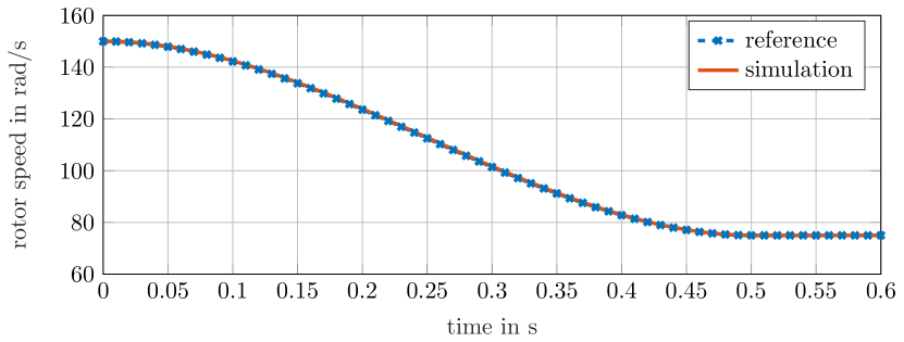
Figure 1: Open-loop simulation result ($T_{s}=10\mathrm{ms}$, as in [13]).

III-B Dynamic Feedback Linearization

In the continuous-time framework, flatness is closely related to the dynamic feedback linearization problem. To be precise, the class of differentially flat systems is equivalent to the class of systems linearizable via endogenous dynamic feedback. A continuous-time dynamic feedback $\dot{z}=\alpha(x,z,v)$ with $u=\beta(x,z,v)$ is said to be endogenous, if there exists a one-to-one correspondence between trajectories of the closed-loop system and trajectories of the original system. As a consequence, $z$ and $v$ can be expressed as functions of $x$, $u$ and time derivatives of $u$.

According to [6], a discrete-time dynamic feedback is said to be endogenous, if its states $z$ and inputs $v$ can be expressed as functions of $x$, $u$ and forward-shifts of $u$. It can be shown that the class of discrete-time systems that is linearizable via endogenous dynamic feedback in the sense of [6] exactly corresponds to the class of forward-flat systems. In the following, we show that also for flat systems according to Definition 1 there always exists a linearizing discrete-time dynamic feedback. However, in general the required feedback is not contained within the class of endogenous dynamic feedbacks proposed in [6].

Theorem 3

A flat system (1) can be linearized by a dynamic feedback

$$\begin{aligned} z^{+}&=\alpha(x,z,v)\,,\end{aligned}\hphantom{a} u=\beta(x,z,v)$$ (23)

with the following properties:

1. The closed-loop system is submersive.

2. The trajectories of the closed-loop system are in one-to-one correspondence to the trajectories of the original system.

Proof:

The fact that the parameterizing map (15) is a submersion implies that also the parameterization $F_{x}$ is a submersion. Consequently, there exists a map $z=F_{z}(y,\dots,y_{[R-1]})$, such that the combined map $(x,z)=(F_{x},F_{z}):=F_{xz}$ forms a diffeomorphism, with $\dim(z)=p\leq mr-n$. We define the map $\Phi(y,\dots y_{[R]})$ given by

$$x =F_{x}(y,\dots,y_{[R-1]})\,, v =y_{[R]}\,,$$ (24)

$$z =F_{z}(y,\dots,y_{[R-1]})$$

and its inverse $\hat{\Phi}(x,z,v)$ given by

$$\begin{array}[]{c}\begin{aligned} (y,\dots,y_{[R-1]})&=\hat{F}_{xz}(x,z)\,,\end{aligned}\end{array} y_{[R]}=v\,.$$ (26)

Based on (26), a linearizing dynamic feedback is given by

$$\begin{aligned} z^{+}&=\delta_{y}(F_{z})\circ\hat{\Phi}(x,z,v)\,,\end{aligned} u=F_{u}\circ\hat{\Phi}(x,z,v)\,,$$ (27)

as we prove next by transforming the closed-loop dynamics

$$\begin{aligned} x^{+}&=f(x,F_{u}\circ\hat{\Phi}(x,z,v))\\ z^{+}&=\delta_{y}(F_{z})\circ\hat{\Phi}(x,z,v)\end{aligned}$$ (28)

into Brunovsky normal form. With the state-transformation $(x,z)=F_{xz}(y,\dots,y_{[R-1]})$ and the input-transformation $v=y_{[R]}$ we get

$$(y^{+},\dots,y_{[R-1]}^{+})=\hat{F}_{xz}\circ\left[\begin{array}[]{c}f(x,F_{u}\circ\hat{\Phi}(x,z,v))\\ \delta_{y}(F_{z})\circ\hat{\Phi}(x,z,v)\end{array}\right]\circ\Phi\,,$$

which can be rewritten as

$$\begin{aligned} (y^{+},\dots,y_{[R-1]}^{+})&=\hat{F}_{xz}\circ\left[\begin{array}[]{c}f(F_{x},F_{u})\\ \delta_{y}(F_{z})\end{array}\right]\,.\end{aligned}$$ (29)

Since the parameterization (15) satisfies the system equations identically, by substituting $F$ into $\delta(x)=f(x,u)$ we get the relation $\delta_{y}(F_{x})=f(F_{x},F_{u})$ and may rewrite (29) as

$$(y^{+},\dots,y_{[R-1]}^{+})=\hat{F}_{xz}\circ\left[\begin{array}[]{c}\delta_{y}(F_{x})\\ \delta_{y}(F_{z})\end{array}\right]\,.$$

Due to $\hat{F}_{xz}\circ(\delta_{y}(F_{x}),\delta_{y}(F_{z}))=\delta_{y}(\hat{F}_{xz}\circ(F_{x},F_{z}))$, and since per definition $\hat{F}_{xz}\circ(F_{x},F_{z})$ yields identically $(y,\dots,y_{[R-1]})$, the Brunovsky normal form follows as

$$(y^{+},\dots,y_{[R-1]}^{+})=\delta_{y}(y,\dots,y_{[R-1]})=(y_{[1]},\dots,y_{[R]})\,.$$

Since the closed-loop system can be transformed into Brunovsky normal form, the dynamic feedback (27) preserves both submersivity and reachability, and it remains to show condition (b). Due to (24) we have a one-to-one correspondence between trajectories of the closed-loop system and trajectories of the trivial system. However, the trajectories of the trivial system are by the definition of flatness in one-to-one correspondence to the trajectories of the original system, which completes the proof. ∎

Since two submersive systems (1) with a one-to-one correspondence between their trajectories are either both flat or non-flat, we get the following corollary.

Corollary 2

Applying a discrete-time dynamic feedback (23) with the properties (a) and (b) of Theorem 3 does not affect the flatness of a system (1).

In contrast to a continuous-time endogenous dynamic feedback, the additional condition (a) is required. Otherwise, the reachability and hence also flatness could be lost. The difference to the notion of discrete-time endogenous dynamic feedback introduced in [6] is that in our case the variables $z$ and $v$ of (23) may depend on both forward- and backward-shifts $(\dots,\zeta_{[-1]},x,u_{[1]},\dots)$ of the system variables.

Remark 4

In the classical dynamic feedback linearization problem, the one-to-one correspondence between trajectories of the closed-loop system and the original system is not required. Thus, the linearizing output of the closed-loop system can possibly not be expressed in terms of forward- and backward-shifts of the original system variables.

IV Conclusion

In this contribution, we have investigated the extension of the notion of discrete-time flatness to both forward- and backward-shifts. We have shown that adding backward-shifts fits very nicely with the concept of one-to-one correspondence of solutions of the original system and a trivial system, as it is well-known from the continuous-time case. Even with backward-shifts, reachability and controllability still hold and trajectories can be planned in a straightforward way. Furthermore, such systems can be linearized by a particular subclass of dynamic feedbacks. Thus, from an application point of view, the basic properties of forward-flat systems are preserved. Since we expect that the class of flat systems in the extended sense including backward-shifts is significantly larger than the class of forward-flat systems, this opens many new perspectives for practical applications as illustrated by the presented induction motor. Future research will deal with the systematic construction of flat outputs and finding necessary and/or sufficient conditions as they already exist for forward-flat systems. Another open question, which is motivated by the continuous-time case, is whether the class of flat systems is only a subset of or equivalent to the class of systems linearizable by dynamic feedback, see Remark 4.

References

- [1] M. Fliess, J. Lévine, P. Martin, and P. Rouchon, “Flatness and defect of non-linear systems: introductory theory and examples,” International Journal of Control, vol. 61, no. 6, pp. 1327–1361, 1995.
- [2] ——, “A Lie-Bäcklund approach to equivalence and flatness of nonlinear systems,” IEEE Transactions on Automatic Control, vol. 44, no. 5, pp. 922–937, 1999.
- [3] A. Kaldmäe and Ü. Kotta, “On flatness of discrete-time nonlinear systems,” in Proceedings 9th IFAC Symposium on Nonlinear Control Systems, 2013, pp. 588–593.
- [4] H. Sira-Ramirez and S. Agrawal, Differentially Flat Systems. New York: Marcel Dekker, 2004.
- [5] B. Kolar, A. Kaldmäe, M. Schöberl, Ü. Kotta, and K. Schlacher, “Construction of flat outputs of nonlinear discrete-time systems in a geometric and an algebraic framework,” in Proceedings 10th IFAC Symposium on Nonlinear Control Systems, 2016, pp. 808–813.
- [6] E. Aranda-Bricaire and C. Moog, “Linearization of discrete-time systems by exogenous dynamic feedback,” Automatica, vol. 44, no. 7, pp. 1707–1717, 2008.
- [7] B. Kolar, M. Schöberl, and J. Diwold, “Differential-geometric decomposition of flat nonlinear discrete-time systems,” arXiv e-prints, 2019, arXiv:1907.00596 [math.OC].
- [8] B. Kolar, J. Diwold, and M. Schöberl, “Necessary and sufficient conditions for difference flatness,” arXiv e-prints, 2019, arXiv:1909.02868v2 [math.OC].
- [9] J. Diwold, B. Kolar, and M. Schöberl, “A normal form for two-input forward-flat nonlinear discrete-time systems,” International Journal of Systems Science, 2021.
- [10] P. Guillot and G. Millérioux, “Flatness and submersivity of discrete-time dynamical systems,” IEEE Control Systems Letters, vol. 4, no. 2, pp. 337–342, 2020.
- [11] H. Nijmeijer and A. van der Schaft, Nonlinear Dynamical Control Systems. New York: Springer, 1990.
- [12] J. Grizzle, “Feedback linearization of discrete-time systems,” in Analysis and Optimization of Systems, ser. Lecture Notes in Control and Information Sciences, A. Bensoussan and J. Lions, Eds. Berlin: Springer, 1986, vol. 83, pp. 273–281.
- [13] P. Martin and P. Rouchon, “Flatness and sampling control of induction motors,” IFAC Proceedings Volumes, vol. 29, no. 1, pp. 2786–2791, 1996.
- [14] J. Chiasson, “A new approach to dynamic feedback linearization control of an induction motor,” IEEE Transactions on Automatic Control, vol. 43, pp. 391–397, 1998.