On simplification of Dual-Youla approach for closed-loop identification
Abstract
The dual Youla method for closed loop identification is known to have several practically important merits. Namely, it provides an accurate plant model irrespective of noise models, and fits inherently to handle unstable plants by using coprime factorization. In addition, the method is empirically robust against the uncertainty of the controller knowledge. However, use of coprime factorization may cause a big barrier against industrial applications. This paper shows how to derive a simplified version of the method which identifies the plant itself without coprime factorization, while enjoying all the merits of the dual Youla method. This simplified version turns out to be identical to the stabilized prediction error method which was proposed by the authors recently. Detailed simulation results are given to demonstrate the above merits.
keywords:
system identification, closed loop identification, coprime factorization, linear systems1 Introduction
Closed loop identification is often inevitable in real world. When the plant to be estimated is unstable in open loop, the I/O data should be collected in closed loop setting. Even if it is stable, it is often the case that the plant must be operated in the presence of feedback controller due to safety and economic reasons. Since it is well known that closed loop identification is difficult due to the correlation between the measurement noise and the input, various methods have been proposed so far to overcome the difficulty (see e.g., Van den Hof and Schrama (1995); Forssell and Ljung (1999); van der Veen et al. (2013)).
These methods may be classified as direct and indirect ones. Direct methods ignore the presence of feedback controller, and identify the plant model using the I/O data only. However, they require the exact knowledge of noise model structure. It is not easy to obtain such knowledge in most cases. Instead, the knowledge of feedback controller is often available. In this case, it would be reasonable to exploit the knowledge. Indirect methods use the exact controller knowledge to obtain an accurate plant model subject to noise under modeling. Most of them identify the closed loop transfer function first, then the plant model is calculated. In order to obtain accurate plant model, the exact knowledge of the controller is necessary. Furthermore, it requires some techniques to identify unstable plants as pointed out by Forssell and Ljung (2000). Though this fact may not be well recognized, this could be a serious problem in some cases.
Among various indirect methods, we focus on the dual Youla method (Hansen and Franklin (1988); Hansen et al. (1989); Van den Hof and de Callafon (1996)). The method transforms the original closed loop identification into an open loop identification for a stable system by using Youla parametrization based on coprime factorization. This method is inherently robust in identifying unstable plants, irrespective of the noise models. Moreover, it is not sensitive to the accuracy of the controller knowledge, which is very important in practice. There are few methods which enjoy both of these merits, except Agüero et al. (2011). Unfortunately, the dual-Youla method has some problems to overcome. First, it relies on coprime factorization over a proper stable rational ring (see Vidyasagar (2011)). Since most engineers in industry are not familiar with such coprime factorization, this could be a big barrier for them to use the dual-Youla method. Also, the identified plant model tends to be of high order because of Youla parametrization (unless adopting some technique like the tailor-made parametrization proposed by van Donkelaar and Van den Hof (2000)). Second, the method tries to identify a virtual system (so called Youla parameter) instead of the plant itself. This is not transparent at all conceptually. Furthermore, it is difficult to exploit prior information of the plant (e.g, integrator type, system order) even if it is available.
The purpose of this paper is to derive a simplified identification method which overcomes the above drawbacks based on the dual Youla method for MIMO systems. More precisely, starting from the dual Youla method, we show how to identify the plant itself without coprime factorization.This method turns out to be nothing but the stabilized PEM (prediction error method) developed by Maruta and Sugie (2018). Furthermore, we will demonstrate the merit to identify the plant itself without coprime factorization, and the robustness against the uncertainty of the controller knowledge and noise model structure through detailed simulation.
2 Dual Youla method
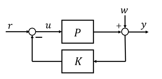
First, we briefly describe the dual Youla method. Consider the closed loop system shown in Fig 1, which is described by
| (1) | ||||
| (2) |
where is the plant to be identified with -dimensional output and -dimensional input which may be unstable, and is contaminated by noise which could be colored. is a given stabilizing controller, and is an -dimensional exogenous signal. We will identify based on the information of the I/O data with the knowledge of .
Let and be lcf (left coprime factorization) and rcf (right coprime factorization) of over the proper stable rational ring , respectively. Since is stabilized by ,
| (3) |
holds for some , where and satisfy the Bézout identity
| (4) |
Hence the plant can be represented by the block diagram shown in Fig. 2.
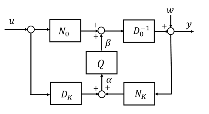
Let and be the input and output of , respectively. Then it is easy to see that
| (5) | ||||
| (6) |
hold. Let , then we have
| (7) |
Here both and can be calculated from I/O data . Moreover, is not correlated with noise at all because
| (8) |
holds from (2) and (5). This is very important. Hence we can obtain consistent model of from and in an open loop setting as shown in Fig. 3. Consequently, we can identify the (possibly unstable) plant in closed loop by using the conventional open loop identification technique.
Remark 1: The dual Youla method in MIMO case can be found in Van den Hof and de Callafon (1996); Forssell and Ljung (1999). However, they use rcf of . So the block-diagram representation is different from the original one in Hansen and Franklin (1988). By using lcf representation of , Fig. 2 is the same as Hansen’s one. This enables us to argue the simplification of the dual Youla method as shown below.
Remark 2: Let be any controller which stabilizes , and and be lcf and rcf of , respectively. Then the above argument still holds. Hence, the original closed loop identification is transformed to an open loop identification of a stable . However, in this case, (8) should be replaced by
This implies that is correlated with noise in case of . As a result, the accuracy of the model may be degraded due to this correlation. However, the effect of is not so direct as the conventional indirect methods. This might give an intuitive reason why the dual Youla method is not so sensitive with respect to the controller accuracy. The numerical example given later supports this insensitivity.
3 Simplification without coprime factorization
The above idea is very nice. Furthermore, it is known that the method works well even if the controller knowledge is not so accurate. However, there are some drawbacks. Since the model of is calculated from (3) with , the plant order tends to be higher. Though there are infinitely many ways of coprime factorization, how to choose them is not clear. Above all, most engineers are not familiar with coprime factorization over the proper stable rational ring. So, it is not easy for them to use this method. From these observations, we consider a way to identify the plant itself directly in the same spirit of the dual Youla method in what follows.
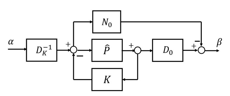
Let be the identified model and be the corresponding plant model, namely
| (9) |
Then we have
| (10) |
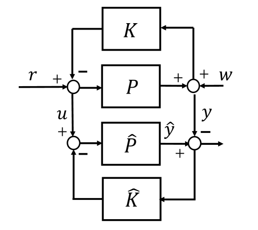
This corresponds to the block diagram shown in Fig. 4. Since hold, the bock-diagram can be transformed into Fig. 5.
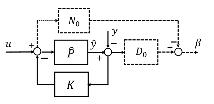
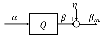
Now the closed loop part consisting of is stable and the input of is not correlated with noise as in the dual Youla method, we can identify the model from by minimizing, e.g.,
| (11) |
This turns out to be nothing but the stabilized PEM (in the case of ) introduced by Maruta and Sugie (2018) which is shown in Fig. 6.
4 Numerical examples
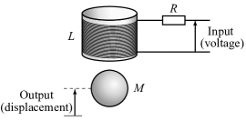
We will demonstrate the effectiveness of the simplified identification method (i.e, stabilized PEM) through a numerical example. The example shown here is based on a linearized model of the magnetic levitation system (see Fig. 7) and controller given in Sugie et al. (1993). The system and controller are described by
| (12) | ||||
| (13) | ||||
| (14) | ||||
| (15) |
where denotes the differential operator. Since it is known that the mag. lev. system is order of three without any zeros in continuous-time, we try to estimate the four parameters . The closed-loop system for data acquisition is described by
| (16) | ||||
| (17) |
where the input of is the voltage applied to the electromagnet coil; the output is the displacement of the steel ball; and is the target displacement and excites the system for identification. The measurement noise and the disturbance are sampled from the standard normal distribution at regular sampling intervals , and are kept for the interval.
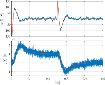
An example of I/O data sampled for identification is shown in Fig. 8. Here, the target displacement was set to a pulse signal with a width of and a height of . These signals are sampled at intervals , and the first-order held signal is used to compute the prediction error with and . And, the model is obtained by minimizing the stabilized prediction error (the output of the system in Fig. 6) with respect to the parameter estimate .
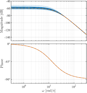
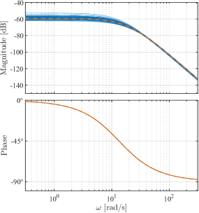
Applying the proposed identification method to 100 sets of I/O data, 100 sets of frequency responses of the models are obtained and are shown as blue lines in Fig. 9. In the figure, the dashed orange line is the true characteristics of the target system, and the red solid line shows the result obtained from I/O data without disturbance and noise (red lines in Fig. 8). To minimize the prediction error about , the Particle Swarm Optimization implementation included in the Global Optimization Toolbox of MATLAB 2020b is used.

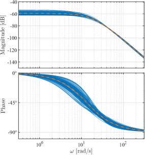
To check the sensitivity to the difference between and , the results obtained using the PID controller
| (18) |
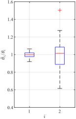
which is different from , as virtual controller are shown in Fig. 9. Also, the distributions of the obtained estimates are shown in Fig. 10 as a box plot.
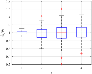
These results show that the stabilized PEM produces a fairly good model, and there is no significant bias in the parameter estimates, as seen in Fig. 10.
For comparison, we also apply a direct method with well-established (discrete-time) models
(with sampling period ), that is,
ARX model:
| (19) |
ARMAX model:
| (20) |
Here,
| (21) | ||||
| (22) | ||||
| (23) |
are polynomials of the unit time delay operator , and is the order of the polynomials. The model parameters , , , , , , and , , are obtained by minimizing the prediction error . The order of each model is determined based on AIC. For the implementation of the conventional methods, we used the ones provided in System Identification Toolbox of MATLAB 2020b with the default settings.
Here, one hundred identification attempts were made for the I/O data that is identical to that for the stabilized PEM, and the frequency response of the transfer function from to of each estimated model is shown as a blue line in Fig. 11. The dashed orange line in the figure is the true characteristics of the target system, and the red solid line shows the result obtained from I/O data without disturbance and noise (red lines in Fig. 8).
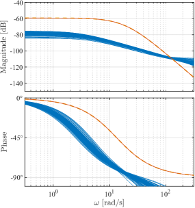
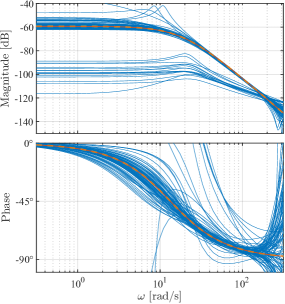
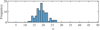
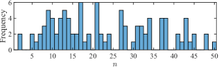
As for the order of the model , the one with the smallest AIC is selected for each data, and the histogram of the selected order is shown in Fig. 12.
The results show that the stabilized PEM produces better models than the direct methods, which can not use the information on the stabilizing controller.
In practical applications, one often wants to obtain a good model by performing system identification based on a gray box model that reflects prior information of the target system. We next confirm the effectiveness of the stabilized PEM in such case.
In this example, based on the physical structure of the magnetic levitation system, we can also consider a gray box model of the following structure:
| (24) | ||||
| (25) |
Here, and are the resistance and inductance of the electromagnet, respectively; is mass of the ball; and are constants related to the electromagnetic force at the equilibrium point. Since direct measurements are possible for , and , our problem here is to estimate and while assuming , and are given.
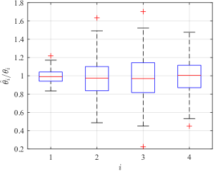
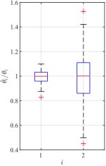
The results obtained based on this gray box model from the aforementioned data are shown in Figs. 13 and 14. As can be seen by comparing Figs. 9 and 13, the variance of the estimates is effectively reduced by using the known information about the structure. Also, the results are not much affected by the choice of the virtual controller .
5 Conclusion
This paper has shown how to derive a simplified version of the dual Youla method which identifies the plant itself (instead of Youla parameter ) without coprime factorization, while enjoying all the merits (such as robustness against both controller parameter uncertainty and noise model structure, and easiness to handle unstable plants) of the dual Youla method. This simplified version turned out to be identical to the stabilized PEM which was proposed by the authors recently. Since coprime factorization nor any special identification technique is not necessary at all, it is easy for most engineers (i.e., non-experts on identification) to use it with numerical optimization. Detailed simulation results have been given to demonstrate the above merits.
References
- Agüero et al. (2011) Agüero, J.C., Goodwin, G.C., and Van den Hof, P.M.J. (2011). A virtual closed loop method for closed loop identification. Automatica, 47(8), 1626 – 1637. 10.1016/j.automatica.2011.04.014.
- Forssell and Ljung (1999) Forssell, U. and Ljung, L. (1999). Closed-loop identification revisited. Automatica, 35(7), 1215 – 1241. 10.1016/S0005-1098(99)00022-9.
- Forssell and Ljung (2000) Forssell, U. and Ljung, L. (2000). Identification of unstable systems using output error and box-jenkins model structures. IEEE Transactions on Automatic Control, 45(1), 137–141. 10.1109/9.827371.
- Hansen and Franklin (1988) Hansen, F.R. and Franklin, G.F. (1988). On a fractional representation approach to closed-loop experiment design. In Proceedings of 1988 American Control Conference, 1319–1320. 10.23919/ACC.1988.4789924.
- Hansen et al. (1989) Hansen, F., Franklin, G., and Kosut, R. (1989). Closed-loop identification via the fractional representation: Experiment design. In Proceedings of 1989 American Control Conference, 1422–1427.
- Maruta and Sugie (2018) Maruta, I. and Sugie, T. (2018). Stabilized prediction error method for closed-loop identification of unstable systems. IFAC-PapersOnLine, 51(15), 479 – 484. 10.1016/j.ifacol.2018.09.191. 18th IFAC Symposium on System Identification SYSID 2018.
- Sugie et al. (1993) Sugie, T., Simizu, K., and Imura, J. (1993). control with exact linearization and its application to magnetic levitation systems. IFAC Proceedings Volumes, 26(2, Part 1), 47–50. 12th Triennal World Congress of the International Federation of Automatic Control.
- Van den Hof and de Callafon (1996) Van den Hof, P.M.J. and de Callafon, R.A. (1996). Multivariable closed-loop identification: from indirect identification to dual-youla parametrization. In Proceedings of 35th IEEE Conference on Decision and Control, volume 2, 1397–1402 vol.2. 10.1109/CDC.1996.572706.
- Van den Hof and Schrama (1995) Van den Hof, P.M. and Schrama, R.J. (1995). Identification and control — closed-loop issues. Automatica, 31(12), 1751 – 1770. Trends in System Identification.
- van der Veen et al. (2013) van der Veen, G.J., van Wingerden, J., Bergamasco, M., Lovera, M., and Verhaegen, M. (2013). Closed-loop subspace identification methods: an overview. IET Control Theory Applications, 7(10), 1339–1358. 10.1049/iet-cta.2012.0653.
- van Donkelaar and Van den Hof (2000) van Donkelaar, E.T. and Van den Hof, P.M. (2000). Analysis of closed-loop identification with a tailor-made parameterization. European Journal of Control, 6(1), 54 – 62. 10.1016/S0947-3580(00)70910-1.
- Vidyasagar (2011) Vidyasagar, M. (2011). Control System Synthesis: A Factorization Approach. Morgan & Claypool Publishers, 1st edition.