Generalized Feynman-Kac Formula under volatility uncertainty
Abstract
In this paper we provide a generalization of a Feynmac-Kac formula under volatility uncertainty in presence of a linear term in the PDE due to discounting. We state our result under different hypothesis with respect to the derivation given by Hu, Ji, Peng and Song (Comparison theorem, Feynman-Kac formula and Girsanov transformation for BSDEs driven by G-Brownian motion, Stochastic Processes and their Application, 124 (2)), where the Lipschitz continuity of some functionals is assumed which is not necessarily satisfied in our setting. In particular, we show that the -conditional expectation of a discounted payoff is a viscosity solution of a nonlinear PDE. In applications, this permits to calculate such a sublinear expectation in a computationally efficient way.
Keywords:
Feynmac-Kac formula, sublinear conditional expectation, nonlinear PDEs
Mathematics Subject Classification (2020): 35K55, 60G65, 60H30
1 Introduction
In this paper we provide a Feynman-Kac formula under volatility uncertainty to include an additional linear term in the associated PDE due to discounting. The presence of the linear term in the PDE prevents the conditions under which a Feynman-Kac formula in the -setting is proved in [11]. Up to our knowledge, there are no contributions in the literature where such a relation between -conditional expectation and solutions of (nonlinear) PDEs is given in a setting not satisfying the hypothesis of [11]. Here, we establish for the first time a relation between nonlinear PDEs and -conditional expectation of a discounted payoff. We introduce a family of fully nonlinear PDEs identified by a regularizing parameter with terminal condition at time , and obtain the -conditional expectation of a discounted payoff as the limit of the solutions of such a family of PDEs when the regularity parameter goes to zero. Using a stability result, we can prove that such a limit is a viscosity solution of the limit PDE. Therefore, we are able to show that the -conditional expectation of the discounted payoff is a solution of the PDE.
More specifically we consider the -setting introduced in [18], a -Itô process and the -conditional expectation
| (1.1) |
for any . Here is a real-valued function, supposed to be continuous with polynomial growth, which may represent the payoff of an interest rate derivative or of a life insurance liability in applications.
In the classical framework, the well known Feynman-Kac representation theorem establishes -under some integrability conditions on their coefficients- a connection between SDEs and parabolic PDEs by the formula
| (1.2) |
where is a given payoff function, is an Itô process solution to a given SDE and is the unique classical solution to a parabolic PDE associated to the SDE solved by , with final condition .
An analogous of a Feynman-Kac formula within the framework of -expectation is given in Theorem 4.5 of [11]. This result connects the solution of a -BSDE to the unique viscosity solution of a fully nonlinear PDE, whose nonlinearity is given by a term that depends on the function representing the uncertainty about the volatility. The authors are able to deal with viscosity (i.e., non necessarily classical) solutions to the associated PDEs assuming the Lipschitz continuity of the coefficients of the -BSDE. However, due to the presence of the discounting term in (1.1), these conditions are not satisfied in our framework, so that we cannot apply this formula directly.
In the setting of short rate models under a fixed probability measure, a Feynman-Kac formula is proposed in [7] which derives (1.2) starting from the PDE associated to the SDE solved by , and proving that its solution can be seen as the conditional expectation of the discounted payoff. On the contrary in [11], the authors start from a -conditional expectation and prove that this solves a fully nonlinear PDE. In the present work, we aim to extend the approach in [7] to the -setting.
In particular, we assume that is quasi-surely strictly positive and solves a given -SDE, with Lipschitz coefficients. We then consider a fully nonlinear, non-degenerate parabolic PDE associated to this -SDE. This PDE contains a linear term due to discounting, which requires to consider a quasi-surely strictly positive process in order to apply the associated PDE theory from [14]. In general such a PDE does not admit a classical solution. For this reason, we substitute the coefficients of the original PDE with some bounded and cut-off functions depending on a parameter . In this way, we are able to show that the approximated PDE admits a viscosity solution defined on an unbounded domain, which is additionally inside a bounded domain depending on . We can then apply the -version of the Itô’s formula to prove the martingale property of the stopped process defined by for every , where the stopping time is the exit time from . We then show that the sublinear conditional expectation in can be obtained as the limit of for going to zero for any , see Theorem 4.15. This is obtained by using a probabilistic approach exploiting the martingale property of , , together with some properties of the family of stopping times . Using a stability result, we are then able to prove that is a viscosity solution of the original PDE, getting the representation
| (1.3) |
for any . For this first analysis we assume to be bounded, then we extend these results to the case when has polynomial growth. In particular, we consider a family of bounded functions approximating , use a version of the dominate convergence theorem for the -setting and employ a stability result in order to get Theorems 4.27 and 4.28, which are the main outcomes of the paper. Note that in general it is not possible to prove uniqueness of the viscosity solution. However, we provide an error estimate in approximating the -expectation by the unique viscosity solution for any and any bounded .
These findings are also relevant for financial applications, in particular for the pricing of contingent claims in fixed income markets or in insurance modeling under volatility uncertainty, a topic which has been investigated in [9], [8] and [10] in the -setting and in [2] by considering nonlinear affine processes under model uncertainty which were introduced in [6].
In order to perform the analysis illustrated above, we have to use both stochastic calculus in the -setting and the theory of nonlinear PDEs. In particular, one of the main technical difficulties is to prove the existence of a solution to the regularized PDEs which is also on a bounded domain depending on the regularizing parameter, by following [14]. For the reader’s convenience, we recall some results of [14] in Section 3 on regularity of solutions of nonlinear PDEs, whereas we devote Section 2 to an introduction to the -setting and to the theory of stopping times in this framework, see [4], [11], [18], [19], [16]. Section 4 contains the main contributions of the paper about a Feynmac-Kac formula in the -setting, see Theorems 4.22 and 4.28. Here, a consistent effort is devoted to verify that the stopped process is well defined and a -martingale for any , and to show that (1.1) is equal to the limit of solutions of the regularized PDEs when goes to zero.
It is also crucial to obtain a stability result in order to prove that such a limit is itself a solution of the limit PDE.
In Section 5 we solve numerically the PDE and plot the approximated value of the -expectation in (1.3), for some choices of the payoff functions and of the coefficients of the -SDE identifying the underlying. This is also a further contribution since it is well known that the strong law of large numbers in the -setting differs from the one in the classical framework, see Theorem 2.4.1 in [18], and this may cause some issues in the application of Monte-Carlo algorithms to approximate -expectations, see for example [20].
2 -Setting
We now recall the basic concepts for the -setting based on [18].
Definition 2.1.
Let be a given set and let be a vector lattice of -valued functions defined on such that for all constants , and if . is considered as the space of random variables. A sublinear expectation on is a functional satisfying the following properties: for all , we have
-
1.
Monotonicity: If then .
-
2.
Constant preserving: .
-
3.
Subadditivity: .
-
4.
Positive homogenity: , .
The triple is called a sublinear expectation space.
Let be a space of random variables such that if , then
where denotes the linear space of functions satisfying for each ,
| (2.1) |
for some depending on . In the following we only consider random-variables with values in i.e., we fix .
We now introduce the -Brownian motion by giving the following definitions.
Definition 2.2.
A random variable is said to be independent from a random variable if , for .
Definition 2.3.
Two random variables and are identical distributed if for all . In this case, we write .
Definition 2.4.
A random variable in a sublinear expectation space is called -normal distributed if for each it holds
where is an independent copy of . The letter denotes the function defined by
| (2.2) |
From now on we assume that there exists such that for all with we have
| (2.3) |
Condition (2.3) is called the uniformly elliptic condition.
Definition 2.5.
Let be a given monotonic and sublinear function. A stochastic process on a sublinear expectation space is called a -Brownian motion if it satisfies the following conditions:
-
1.
;
-
2.
for each ;
-
3.
For each the increment is independent of for each and . Moreover, is -normally distributed.
Fix now a time horizon and introduce the space of all -valued continuous paths with . We equip this space with the uniform convergence on compact intervals topology and denote by the Borel -algebra. Moreover, the canonical process on is given by for . For we define and .
Definition 2.6.
Introduce as
for . Then the space is the completion of , , under the norm for .
Next we introduce the definition of the -expectation and the -conditional expectation.
Definition 2.7.
A -expectation is a sublinear expectation on defined as follows: For of the form
we set
where are -dimensional random variables on a sublinear expectation space such that for each , is -normally distributed and independent of .
The corresponding canonical process is a -Brownian motion on the sublinear expectation space .
Definition 2.8.
Let have the representation
Then the -conditional expectation under is defined as
where
The -expectation and the -conditional expectation can be extended to sublinear operators and , , see Section 3.2 in [18].
It is shown in Theorem 6.2.5 in [18] that the -expectation is an upper expectation, i.e., there exists a weakly compact set of probability measures such that
| (2.4) |
Related to this set we introduce the Choquet capacity defined by
| (2.5) |
In the following definitions we introduce the most important spaces we will work with.
Definition 2.9.
For we denote by the space of simple integrands. Specifically, for a given partition of , , we define an element by
where .
Definition 2.10.
For we let be the completion of under the norm , and be the completion of under the norm .
Note that . Similar as in the classical Itô case the integral with respect to is first defined for the simple integrands in by the mapping . Then this mapping can be continuously extended to , see Lemma 3.3.4 in [18]. As in the classical case the quadratic variation of the -Brownian motion is defined as the process with for . The integral with respect to the quadratic variation is introduced first for and then extended to , see Section 3.4 in [18].
Definition 2.11.
A process is called a -martingale (respectively, -supermartingale, -submartingale) if for each , and for each , we have
If in addition it holds also
then is called a symmetric -martingale.
2.1 Exit times in the -setting
In the following we summarize some results given in [16] about exit times for semimartingales in the -setting, which we use in Section 4. In [16], a general nonlinear expectation is considered, however for simplicity we now state the results for the -dimensional -expectation. Moreover, instead of dealing with open sets in we only work with open intervals in .
Let be introduced as in Definition 2.1 and be the weakly compact set of probability measures generating the -expectation as in . Consider a one-dimensional -semimartingale , i.e., suppose that under each , has the decomposition
| (2.6) |
where is a continuous local martingale and a finite variation process. Given an open interval in , define the following exit times
where and denote the complement of and of the closure of in , respectively. Introduce the space
Assumption 2.12.
(Local growth condition (H)) Let be an open interval in . We say that the stochastic process in (2.6) satisfies the local growth condition if the following holds. For each there exists a -null set such that, if satisfies , then there exist some stopping time and constants so that
-
1.
for ;
-
2.
For , on the interval , it holds that
Moreover, these three quantities and can depend on and are supposed to be uniform for all .
We now recall the definition of a quasi-continuous function on a measurable space , see Definition 6.1.26 in [18], and of a quasi-continuous process, see p. 13 in [16]. The capacity is introduced in .
Definition 2.13.
-
1.
A mapping on with values in a topological space is said to be quasi-continuous (q.c.) if for all there exists an open set with such that is continuous.
-
2.
A process is quasi-continuous on if for each , there exists an open set with such that is continuous on .
Proposition 2.14.
Corollary 2.15.
(Corollary 4.8 in [16]) Let be a quasi-continuous stopping time. If is a -martingale, then is still a -martingale.
Proposition 2.16.
Let be a quasi-continuous stopping time. Then for each , we have
Moreover, for any it holds and
By combining Example 5.1(i) and Remark 5.2 from [16], we can characterize under which conditions a solution of a -SDE satisfies Assumption 2.12.
Lemma 2.17.
Let be the unique solution to the -dimensional -SDE
where and satisfy the following conditions:
-
1.
the functions are Lipschitz continuous for all and the functions are continuous for all .
-
2.
is non-degenerate, i.e., there exists such that
Then the process is quasi-continuous and Assumption 2.12 is satisfied.
Proof.
It follows by Example 5.1 (i) and Remark 5.2 of [16]. ∎
Remark 2.18.
Given an open interval in , note that all results stated in this subsection are also valid for the exit times
where is fixed and is a process starting at time , with .
3 Nonlinear PDEs
We here recall some results of [14] which are fundamental for our analysis in Section 4 and add some new properties. Introduce an -valued Borel function . Moreover, let be a (possibly unbounded) open interval of and be a cylindrical domain in , with . We introduce the following notation
Then the parabolic boundary of is defined as . For , the parabolic boundary of is given by
Note that in this paper . Moreover, for all -valued functions with , we use the notation , where denotes the absolute value. This section is devoted to the analysis of conditions that provide the existence of a classic solution to the PDE
| (3.1) | ||||
| (3.2) |
where we set
for the sake of simplicity. In the following we use the notation of [14], where , , have not to be understood as dependent on but only as arguments of .
First, we introduce the sets of functions and for constants .
Definition 3.1.
(Definition 1, Section 5.5 in [14]) Introduce the constants .
-
1.
We say that if the following properties are satisfied:
-
•
for every the function is twice continuously differentiable with respect to ;
-
•
for all and the following inequalities hold:
where we omit the arguments of and its derivatives, and
Moreover, and are here some continuous functions which grow with and , and such that .
-
•
-
2.
We say that if the following properties are satisfied:
-
•
is continuously differentiable with respect to all arguments;
-
•
;
-
•
for each and we have
where is a continuous function growing with and .
-
•
Definition 3.2.
(Definition 1, Section 6.1 in [14]) Introduce the constants and define the set as
We say that if there exists a sequence of functions converging to as at every point of the set such that
-
1.
-
2.
for any the function is infinitely differentiable with respect to and the derivative of any order of the function with respect to is bounded on for any ;
-
3.
there exist constants such that
for all , and .
Note that the following results also hold for .
Theorem 3.3.
(Theorem 3 and 4 in Section 6.4 in [14]) Fix , , , and introduce an interval and a domain . Moreover, let . Suppose that and on . Then Problem (3.1)-(3.2) has a solution with the following properties:
-
1.
, on ;
-
2.
for every , the function belongs to the space where , and the norm of in this space is bounded by a constant depending only on and the function .
- 3.
Theorem 3.4.
(Theorem 5 (d), Section 6.1 in [14]) Fix , , , and introduce an interval and a domain . Fix a set of indices and introduce a function for every , such that are independent of . Then . Moreover, can be replaced by (for any ).
Using Theorem 3.4 several examples of functions in can be constructed.
Example 3.5.
(Example 8, Section 6.1 in [14]) Let be a set of indices. Consider two functions . Suppose that, for every fixed , the functions and are continuously differentiable with respect to , and twice continuously differentiable with respect to , for every fixed .
In addition, let the second derivatives of and with respect to and the first derivatives with respect to be bounded on every set . Moreover, suppose that for all the following inequalities hold:
| (3.3) | |||
| (3.4) | |||
| (3.5) |
where is a continuous function. Finally assume that the inequalities
| (3.6) |
hold for some constants with . Then it can easily be seen that by Theorem 3.4, we have
The constants and introduced in Theorem 3.4 are equal to and , respectively. Moreover, can be chosen to be dependent on , on the functions of which dominate the second derivatives of with respect to and on their first derivatives with respect to on .
We now prove a new result that we use in Section 4.
Lemma 3.6.
Let be a family of Borel measurable functions such that
| (3.7) |
for , , where is an index set. Then the PDE
| (3.8) |
has a solution if and only if the PDE
| (3.9) |
has a solution .
4 Feynman-Kac formula in the -setting
In this section we prove a generalized Feynman-Kac formula in the -setting, in presence of a linear term in the associated PDE. In this way we complement the results of [11] which hold without the linear term in the PDE and under different conditions. More precisely, we do not consider a -BSDE as in [11], but solely a -SDE. Moreover, we do not assume that the payoff function satisfies a Lipschitz condition, and the presence of a discounting term in the -expectation prevents a further Lipschitz assumption involving the coefficients of an associated -BSDE to hold, which is crucial in [11]. On the other hand, we consider some other assumptions on the coefficients of the PDE which are stated in Assumption 4.1, and which are not necessary in [11].
For fixed and consider the -Itô process given by
| (4.1) |
where are deterministic functions such that are Lipschitz-continuous functions for every and are continuous in for every . Our aim is to show that
| (4.2) |
satisfies the PDE
| (4.3) | ||||
| (4.4) |
for and for suitable terminal payoffs satisfying suitable conditions which we discuss in the sequel.
From now on, we work under the following assumption.
Assumption 4.1.
The functions belong to the space . Moreover, is bounded away from zero on every subset , , and for every , . Finally, for all .
As stated in [11] and in Chapter 5 in [18], there exists a unique solution of the -SDE (4.1). Moreover, the following estimates hold for any and :
| (4.5) | ||||
| (4.6) |
where the constant depends on and the Lipschitz constant of . Note that the conditions in Assumption 4.1 on the function are necessary to apply the PDE theory introduced in Section 3. Moreover, the assumption on is necessary for technical reasons in Definition 4.2 and Lemma 4.3.
Definition 4.2.
For fixed define by
for introduced in . Define then for , as given by
| (4.7) |
for . Moreover, define as
| (4.8) |
where is given by
| (4.9) |
setting if and taking such that if . Note that for such a constant exists, as for fixed the function is . Finally, we introduce the function given by
| (4.10) |
Lemma 4.3.
Under Assumption 4.1 the following holds for any :
-
1.
and their first and second derivatives are bounded, for every .
-
2.
, for every , and .
-
3.
is bounded away from zero.
Proof.
Fix and let . By Assumption 4.1, is bounded on and is also bounded for . Therefore, in is bounded. Moreover, and for . Furthermore, for it holds
In particular, , , . Hence, with bounded first and second derivatives for . With similar calculations it can be shown that , with bounded first and second derivatives. Note that by the definition of in and as for all , it follows for all , where is a constant which only depends on . Thus is bounded away from zero. By the definition of in we have with bounded first and second derivatives. ∎
4.1 Feynman-Kac formula for a bounded payoff
In this section we prove a Feynman-Kac formula for a continuous and bounded payoff in (4.4). However, based on the results we find under this assumption and in particular on Theorem 4.22, we are able to extend this result to the case of an unbounded payoff with polynomial growth in Section 4.2.
Assumption 4.4.
The function in (4.4) belongs to and is bounded by a constant .
In order to apply Theorem 3.3, we need the terminal condition of the PDE (3.1)-(3.2) to be bounded and more than twice differentiable on a suitable interval, see the final part of the proof of Proposition 4.8. For this reason, we first approximate with a family of functions satisfying this property.
Definition 4.5.
Let . By the Weierstrass approximation theorem, for any there exists a polynomial function on such that
| (4.11) |
We then define the function as
| (4.12) |
Lemma 4.6.
Proof.
Points 3. and 4. immediately follow by the definition of in (4.12) and since is a polynomial. Moreover, inequality (4.13) is a consequence of (4.11) and the fact that is bounded by the constant .
To prove Point 1., fix and . We want to show that for all there exists a constant such that for all it holds .
Choose and let . Then, since , we have
∎
The following lemma will be useful to derive our convergence results, see the proof of Theorem 4.15.
Lemma 4.7.
Proof.
Set from now on. For we then consider the following PDE
| (4.14) | ||||
| (4.15) |
where is defined as in (2.2).
Condition guarantees that the PDE in - admits a unique viscosity solution , see also Appendix C in [18]. Together with Assumption 4.1, it also guarantees that the PDE in is non-degenerate. Define the function by .
Indeed for it holds
| (4.16) |
where we used for the first inequality and the fact that is bounded away from for the strict inequality in (4.16). Note that in order to ensure non-degeneracy, it would be enough to assume for every . However, we need the restriction to be bounded away from zero later on, see (4.21).
Proposition 4.8.
Proof.
Let . Equation (4.14) can be written as
where
Note that it holds
| (4.17) |
Since is linear in the arguments , it satisfies condition . Thus, by Lemma 3.6, the PDE - has a -solution if and only if the problem
has a -solution. By applying Example 3.5 we now show that for all the function given by
| (4.18) |
is an element in . We set
| (4.19) | ||||
| (4.20) |
Note that by Lemma 4.3 the functions and are continuously differentiable111See computations in Section A.2 in Appendix. with respect to and twice continuously differentiable with respect to .
By Lemma 4.3 we obtain that the second derivatives of and with respect to , i.e., and for , and the first derivative with respect to are bounded on .
We now show that for all , inequalities - are satisfied.
We first prove that
| (4.21) |
for some . By definition of , Assumption 4.1 and Lemma 4.3 this is equivalent to show
| (4.22) |
By condition applied to there exists such that . As , we can find such that the first inequality in holds. Moreover, the second inequality follows by .
Next, we need to find an upper bound for . We have that
| (4.23) |
where the constants exist by Lemma 4.3. Moreover, we used that . Inequality holds, as
| (4.24) |
by Lemma 4.3. We now prove . It holds
| (4.25) |
for a constant which we get from Lemma 4.3. It is obvious that for all we have . Thus, it follows by that , which is a necessary condition in Example 3.5.
For the inequalities in fix such that and choose . As it holds
By Example 3.5 and Theorem 3.4 we can conclude that .
Then Theorem 3.3 and Point 3. of Lemma 4.6 imply the existence of a solution for the PDE - such that and on . Furthermore, by Point 2. of Theorem 3.3 together with Remark 2.1.3 in [18] it follows that is a viscosity solution.
Moreover, we can apply Point 3. of Theorem 3.3, by setting , and , to show that there exists such that .
Indeed, by definition of we have that
as , and by point 4. of Lemma 4.6 that . So we have verified that the conditions of Point 3. of Theorem 3.3 are satisfied.∎
For fixed , define the intervals and the random time
| (4.26) |
where we use the convention . We now state the following result about stopping times.
Lemma 4.9.
Proof.
Fix and define the auxiliary stopping time , so that . By Lemma 2.17 and Remark 2.18 it follows that the process is quasi-continuous, and as is also -adapted, the exit time is a stopping time. Moreover, Assumption 2.12 is satisfied, again by Lemma 2.17 applied to . Thus, it follows directly by Proposition 2.14 that is quasi-continuous as is constant. ∎
Proposition 4.10.
Let satisfy Assumption 4.4 and be the family of functions constructed in Definition 4.5. Given , consider the solution of the -SDE (4.1). Moreover, let Assumption 4.1 hold and be the viscosity solution of the PDE , for given . Then for every , we have that
| (4.27) |
is a -martingale, where the stopping time is given in .
Proof.
Fix . We need to verify that the stopped process with for is well-defined. By definition of in we have to look at
| (4.28) |
Since is quasi-continuous by Lemma 4.9, by Proposition 2.16 we get for
| (4.29) |
Moreover, by Proposition 2.16 it follows that .
By the definition of in we know that for . Moreover, by Proposition 4.8. Thus, we can apply G-Itô’s formula from Theorem 3.6.3 in [18] to the process given by
Note that the conditions of Theorem 3.6.3 in [18] are satisfied as implies that is bounded on and therefore satisfies a polynomial growth condition. Moreover, are bounded, as for any and then Assumption 4.1 implies that are bounded. So we get
| (4.30) | ||||
where we used in that for it holds and
for all by and
For we have
| (4.31) | ||||
| (4.32) | ||||
| (4.33) | ||||
| (4.34) |
where we used Proposition 2.16 in and Remark 3.2.4 in [18] together with the fact that is -measurable in and Proposition 3.3.6. in [18] in .
By Proposition 3.2.9 in [18] for such that , we have
| (4.35) |
We now apply this result to for
with
First, note that , as by Theorem 3.6.3 in [18] and Proposition 2.16. Moreover, by these results it also follows that for all
Thus, as in Proposition 4.1.4 in [18] it holds . As is the solution of the PDE in and for for every , it holds and . As a consequence we have
Thus, it follows by and
| (4.36) |
By Proposition 4.1.4 in [18] we know that for any the process given by
| (4.37) |
is a -martingale. Thus, for it follows
| (4.38) |
where we used for the first equality Remark 3.2.4 in [18]. Note that, as is quasi-continuous, it follows by Corollary 2.15 that is also a -martingale. By applying to and by using the same arguments as in - we get by that
∎
Lemma 4.11.
Proof.
This follows directly by Proposition 4.10 as . ∎
Remark 4.12.
Note that the -conditional expectation on the right-hand side in (4.39) is deterministic, as the process starts in at time .
Lemma 4.13.
Proof.
By Lemma 2.17 we have that is quasi-continuous and therefore quasi-surely finite on . In particular, there exists a quasi-null set such that for all the function , is continuous, and bounded from below from and from above on , as is also quasi-surely positive. Fix . Then there exists such that for every it holds . Therefore, the result follows by the dominated convergence theorem stated in Theorem 3.2 in [12]. ∎
Proposition 4.14.
Proof.
Given , let be the solution to the -SDE (4.1). For any such that it holds
| (4.41) | |||
| (4.42) | |||
| (4.43) |
Note that in we use Proposition 3.2.3 in [18], whereas (4.41) immediately follows from (4.39). For the second term in (4.43) we get
| (4.44) | |||
| (4.45) |
where we use in (4.44) that for we have . For the first term in (4.43) we have
| (4.46) |
Moreover, we get
| (4.47) |
Thus, putting together (4.43)- (4.47) it follows
| (4.48) |
where (4.48) follows because the process is continuous and thus . ∎
Theorem 4.15.
We now establish a Feynman-Kac formula for the -conditional expectations
by providing a stability result on the limits of the modified PDE (4.14)-(4.15) and of Theorem 4.15. To prove the main result of this section, we make use of the following definition of uniform convergence.
Definition 4.16.
For , consider functions . We say that converges locally uniformly for to a function if for every there exists a neighborhood of the point such that converges to uniformly on for , i.e.,
for .
In the sequel we write to indicate convergence of to .
Remark 4.17.
As is a locally compact space, converges to locally uniformly for is equivalent to compactly, i.e., for every compact set , uniformly for .
We start with two lemmas.
Lemma 4.18.
-
1.
For any , define as
and define by
Then locally uniformly for .
-
2.
locally uniformly for .
Proof.
1. Let for . Choose small enough in such that . Let . By the definition of in equations (4.7)-(4.10), we have that for and , for . Moreover, for and . Therefore, for we have
for any The result then follows by Remark 4.17.
2. Let for . Choose small enough in such that . Let . By Definition 4.5 it follows that for any
for . ∎
Lemma 4.19.
For fixed , and , define the stopping times
| (4.50) |
Then for any and , we have
| (4.51) |
and
| (4.52) |
Proof.
First we note that and are quasi-continuos by similar arguments as in Lemma 4.9. For define the exit time
Again by similar arguments as in Lemma 4.9 it follows that is quasi-continuous, as the process is quasi-continuous. We first consider the case . Since and are both quasi-continuous processes, it follows that quasi-surely. Thus, for each we have
which implies that for . Therefore, we get (4.51) by definition of and . If it holds that for all and thus (4.51) holds. The proof of (4.52) is fully analogous. ∎
In order to prove the Feynman-Kac formula in Theorem 4.22, we need to introduce a further hypothesis.
Assumption 4.20.
Remark 4.21.
Note that Assumption 4.20 is very weak, and is for example satisfied if for any and any there exist and such that
| (4.53) |
for any and any . For most common models the latter condition holds (in most cases taking ). Moreover, Assumption 4.20 holds for every solution of a -SDE with time independent coefficients.
Theorem 4.22.
Proof.
In order to get the result, we prove that converges locally uniformly to for . By Remark 4.17, this boils down to prove that for every fixed and , for all there exists a constant such that for every it holds
We have
| (4.57) |
Let . Then for any , for an appropriate choice of , it holds
| (4.58) | |||
| (4.59) | |||
| (4.60) |
Note that both (4.58) and the fact that the term (4.59) is bounded by follow by Definition 4.5.
Remark 4.23.
Note that the presence of the linear term in (4.55) does not allow to apply the comparison principle in Appendix C in [18], which guarantees uniqueness of a viscosity solution. However, Proposition 4.14 provides an estimate for the error in approximating the -expectation with the unique viscosity solution to the PDE for a given .
4.2 Feynman-Kac Formula for unbounded payoffs
In the following we extend the results of Section 4.1 to the case of a continuous payoff function with polynomial growth.
Assumption 4.24.
Let be a constant. The function satisfies a polynomial growth condition of order less or equal in the second variable uniformly in , i.e., there exists a constant only depending on the final time such that it holds
for any .
Assumption 4.24 is now general enough to be satisfied by all the common derivatives on the market. We now prove a Feynman-Kac formula for payoffs satisfying the less restrictive Assumption 4.24 by applying Theorem 4.22 for the (bounded) payoff functions approximating as in Definition 4.5, and then passing to the limit for . The next lemma states that the functions are indeed bounded, and also provides an explicit form for such a bound.
Lemma 4.25.
Proof.
The specific form of the bound given in (4.65) will be crucial to prove Theorem 4.27 and Theorem 4.28. The latter constitutes the main result of the paper. We start by extending the result of Lemma 4.7 to the case when is not bounded.
Lemma 4.26.
Proof.
We have
| (4.68) |
In particular, for any it holds
| (4.69) | |||
| (4.70) | |||
| (4.71) | |||
| (4.72) |
where we use Assumption 4.24 and (4.65) in (4.69). Moreover, we have that (4.70) and (4.71) follow as on the event . In (4.72) we set . Since by (4.5), we can use Proposition 6.3.2 in [18] and Theorem 25 of [5] to get
| (4.73) |
Together with (4.72), this implies that for any there exists such that
| (4.74) |
for any . Moreover, by (4.11) we have
| (4.75) |
for any . For any , by (4.68), (4.74) and (4.75) we get
for any with . ∎
We now get the following result.
Theorem 4.27.
Let satisfy Assumption 4.24 and be the family of functions constructed in Definition 4.5. Given , assume that the process in is quasi-surely strictly positive. Moreover, let Assumptions 4.1 and 4.20 be satisfied. Then there exists a family of viscosity solutions for the PDEs
| (4.76) | ||||
| (4.77) |
for , with the property that
for every .
Proof.
Theorem 4.28.
Proof.
We apply a stability result similar as in the proof of Theorem 4.22. In order to do that, we need to prove that the family introduced in Theorem 4.27 converges locally uniformly to for . This means that for every fixed and , for all there exists a constant such that for every it holds
Let be the family of approximating functions for from Definition 4.5. For we have
| (4.82) |
We now focus on the first term in (4.82). We prove here that for all there exist such that for it holds
| (4.83) |
for all . We have
| (4.84) | |||
| (4.85) | |||
| (4.86) | |||
| (4.87) | |||
| (4.88) |
We used Assumption 4.24 and (4.65) in (4.84) and set in (4.85). Furthermore, (4.86) holds by similar arguments as in Lemma 4.19. Moreover, (4.87) follows by Hoelder’s inequality. For the first term in (4.88) we have
| (4.89) | ||||
| (4.90) |
where we use (4.6) in (4.89) and denotes a suitable constant. Putting together (4.88), (4.90), it follows
| (4.91) | |||
| (4.92) |
for . Here, (4.91) follows as
Moreover, (4.92) holds as is increasing and continuous and by Assumption 4.20. Thus (4.83) holds. Moreover, for the second term in (4.82) for any and any it holds
Thus, we conclude that converges locally uniformly to for . Moreover, by the second point of Lemma 4.18 it follows by the same stability arguments as in the proof of Theorem 4.22 that is a viscosity solution of the PDE (4.80)-(4.81). ∎
Next, we prove a generalization of Proposition 4.10, i.e. we show that the process for defined by
| (4.93) |
is a -martingale. Here, the function is given in (4.79).
Proposition 4.29.
Proof.
First, we prove that for any . Since and
| (4.94) |
it is enough to show that
By the characterization of in Exercise 6.5.2 in [18], we need to show that is a quasi-continuous random variable and that
| (4.95) |
As is a quasi-continuous process, it follows that is a quasi-continuous random variable. Thus, is quasi-continuous by the continuity of and . Moreover, by Assumption 4.24 and by (4.73), we have
We have then proved that . Fix now . By (4.94) we have
| (4.96) |
which shows that satisfies the -martingale property. ∎
In particular, Proposition 4.29 provides the dynamic programming principle
where is given in (4.79).
Remark 4.30.
In financial applications the results derived in Section 4 are especially of interest when models a short rate or default/mortality intensity. In this case, the results in Theorems 4.22 and 4.28 allow to represent the price of a zero-coupon bond with maturity by a solution of a nonlinear PDE. However, compared to the classical case the -SDE in contains an additional term, namely the integral with respect to the quadratic variation of the -Brownian motion. This extra term can be regarded as an additional uncertain drift term, as the process represents mean-uncertainty in the -setting.
Remark 4.31.
Most of the previous results only hold for a quasi-surely strictly positive process in . This assumption is for example satisfied for all process of the form , where is a process such that quasi-surely. In Section 5 we give an example of such a process, namely a generalized version of the exponential Vasicek model.
Remark 4.32.
The aim of this paper is to provide a Feynman-Kac formula in the -setting which allows to numerically compute the following -conditional expectation
To do so, we start from the -SDE in (4.1) under the standard assumption of Lipschitz continuous coefficients in the -setting. To the best of our knowledge there are no general results without the Lipschitz assumption which guarantee existence and uniqueness of the solution for a -SDE. The only contributions dealing with -SDEs with non-Lipschitz coefficients are [1], [15].
In order to model interest rates under model uncertainty there exist two different approaches in the literature. First, [6] introduces non-linear affine processes by considering a family of continuous semimartingale laws as a starting points, such that the differential characteristics are bounded from below and above from affine functions. However, this approach is not applicable in our setting as it does not consider -SDEs. Second, in [9], [8], [10] a HJM framework in the -setting is considered. More specifically, the forward rate dynamics is modeled by a -SDE. However, also here only Lipschitz continuous coefficients in the corresponding -SDEs are considered.
5 Numerical applications
In this section we use an explicit Euler scheme to numerically approximate the solution to the PDE (4.80)-(4.81) for some choices of its coefficients, of the payoff function and of the volatility uncertainty interval . By Theorem 4.28, such solution represents the -expectation of the discounted payoff with underlying given by (4.1).
Remark 5.1.
We choose to numerically solve (4.80)-(4.81) with an explicit Euler scheme in order to avoid artificial boundary conditions, since the domain is unbounded and it is hard to guess a possible behaviour of the solution for large values of the spatial coordinate.
Using the explicit Euler scheme we are of course left with the problem of the stability of the numerical solution. Computing stability conditions in our case appears to be a difficult task, since the PDE is fully nonlinear and with nonconstant coefficients. This goes beyond the scope of this paper and can be object of further investigation. However, for the time discretization step we choose for our numerical simulations, we observe a behavior in line with the theory. For example, the values we find for the classical case for a call option with an underlying following log-normal dynamics agree with the well known analytical formulas.
We focus on two examples.
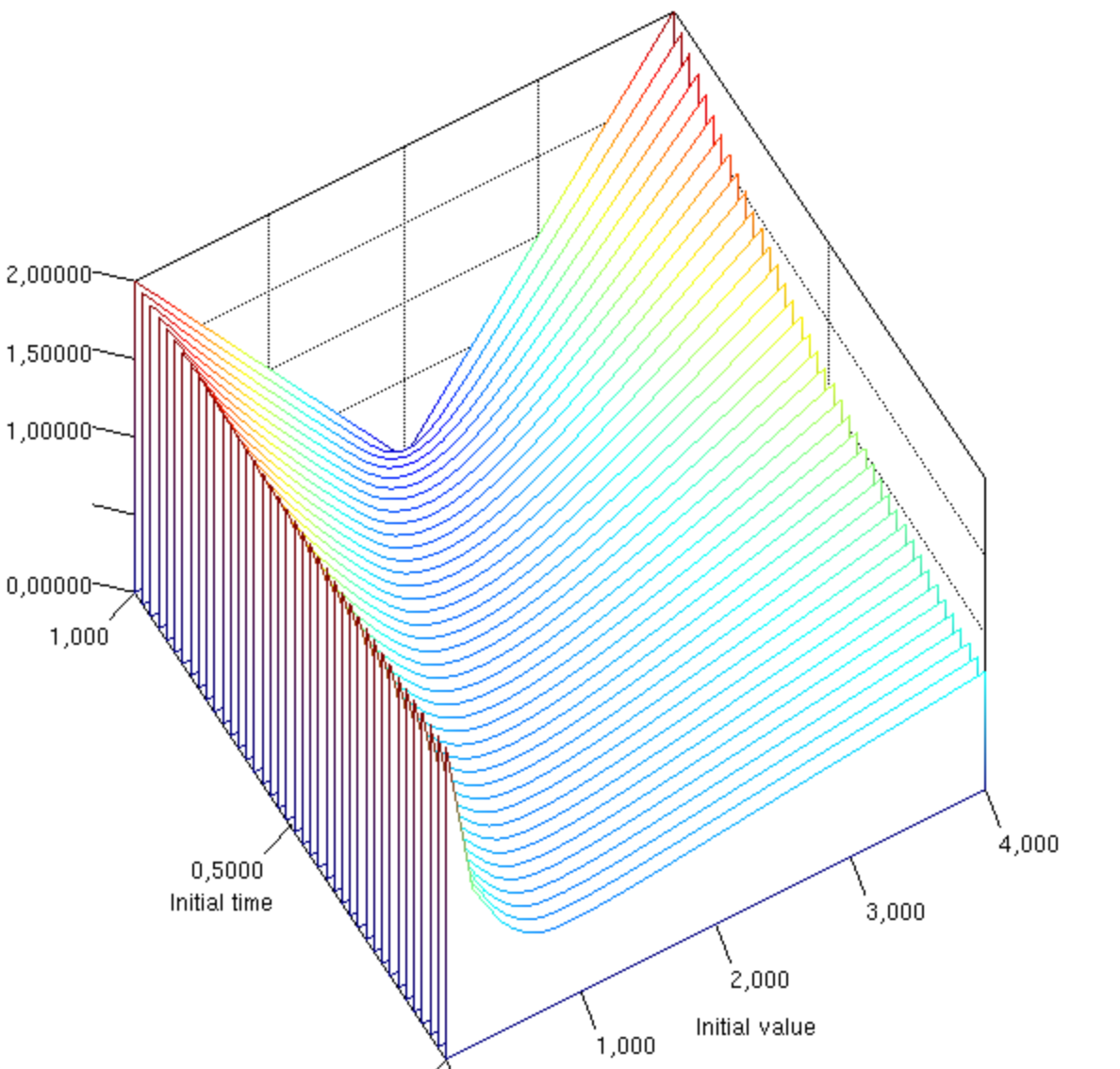
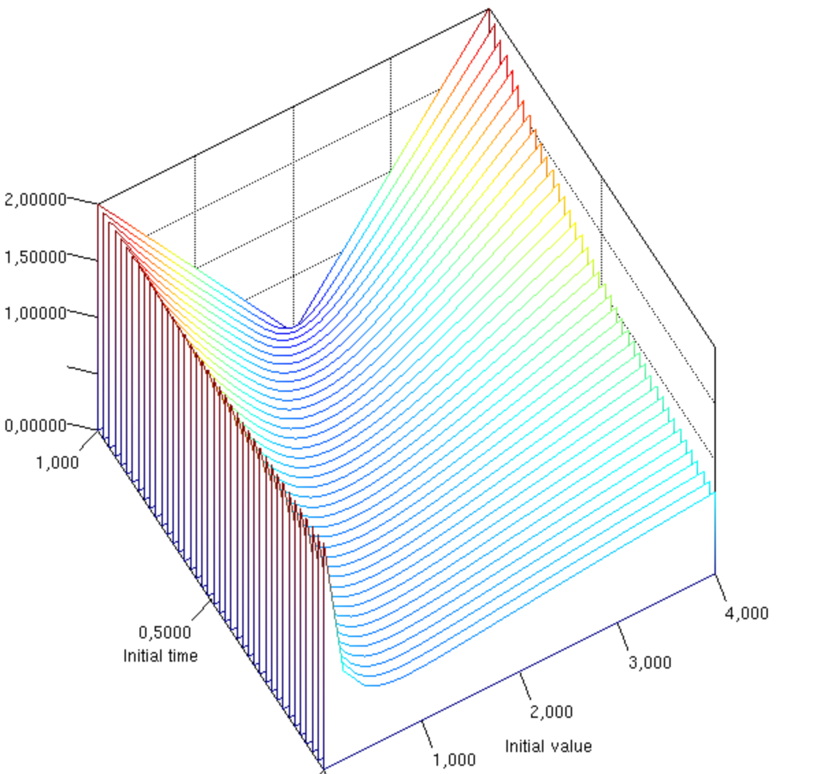
5.1 Dothan model with quadratic variation term
We here consider the stochastic process which follows the -SDE
| (5.1) | ||||
| (5.2) |
with and .
As is quasi-surely strictly positive, we can apply Theorem 4.28 to approximate the -expectation
for a given payoff function satisfying Assumption 4.24, as a numerical solution to the PDE (4.80)-(4.81) associated to (5.1), i.e., with coefficients
We also set
In financial applications, represents the payoff of a call option on (or of a caplet on , if models an interest rate).
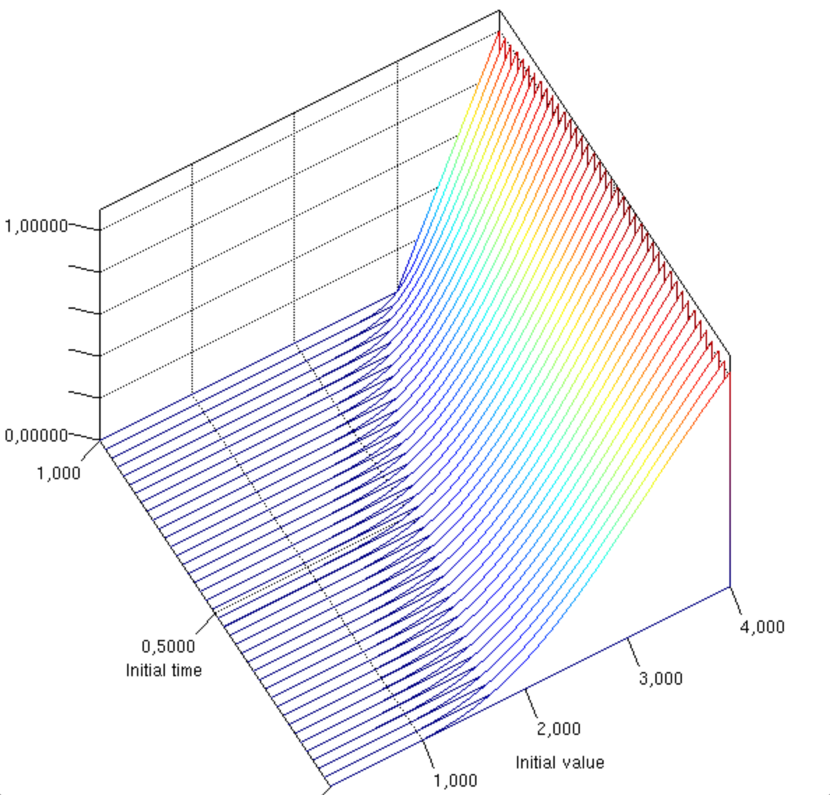
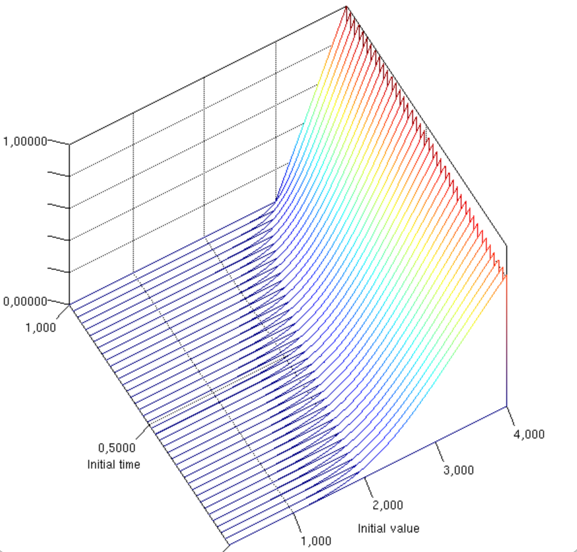
We take parameters , , , , , and let vary in , in . The right boundary of our approximated domain is .
Remark 5.2.
Having to consider a bounded domain represents a further approximation of our solution with respect to the analytic one. As commented above, we avoid to fix artificial boundary conditions since we apply an Explicit Euler scheme. In our plots we represent the approximated solution up to , which is far away from the right boundary of the approximated domain.
Figures 1 and 2 show the values of the approximated solutions for . We note that the values of the approximated expectations are increasing with the uncertainty on the volatility. Moreover, the expectation is higher for and smaller for . This is not surprising at least for the classical case (i.e., when ), where gets just summed to the drift term since .


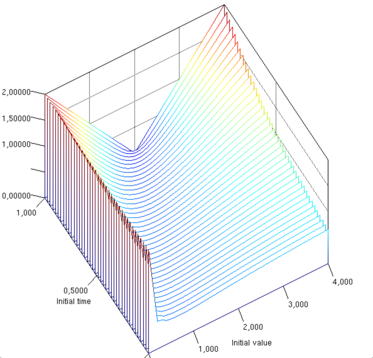
5.2 Exponential Vasicek model with quadratic variation term
Consider now the process given by the -SDE
for , which has a unique solution by Theorem 5.1.3 in [18], and set
for and . Since quasi-surely for any because it is quasi-continuous, is quasi-surely strictly positive for any as required in Theorem 4.15.
We apply the -Itô’s formula to , in order to compute the coefficients of the PDE. Since the function is not bounded on the whole real line, we choose a big enough constant such that and stop the process at stopping times given by
so that using similar arguments as in Lemma 4.9 it follows that is a quasi-continuous stopping time for every and any . Then we have that
| (5.3) |
Note that the SDE (5.3) has non Lipschitz coefficients. However, the existence and uniqueness of follows as . We then numerically solve the PDE (4.80)-(4.81) with
We consider the sum of a call and of a put option with same strike, i.e., we fix the final condition
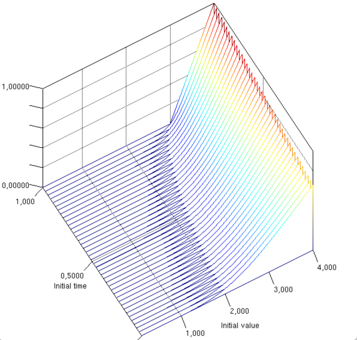
We take parameters , , , , , , . As above, we let vary in . The right boundary of our approximated domain is . Figure 3 shows the values of the approximated solutions for . Again, we note that the values of the approximated expectations is increasing with the uncertainty on the volatility.

Appendix A Computations of the partial derivatives for in Proposition 4.8
Appendix B Risky asset and short rate driven by a -dimensional -Brownian motion
The techniques developed in Section 4 can also be applied to derive a Feynman-Kac formula when the underlying is a -Itô process driven by a -dimensional -Brownian motion. This allows to apply our results for more complex applications such as market models with multiple risk factors or stochastic discounting factors. To illustrate how to generalize our techniques we consider -Itô processes and representing a risky asset and a stochastic interest rate, respectively.
For fixed and consider the -Itô processes , given by
| (B.1) |
and
| (B.2) |
where is a -dimensional -Brownian motion and are deterministic functions such that are continuous in for every and are Lipschitz-continuous functions for every , .
Assumption B.1.
For all the functions belong to the space and belong to the space . Moreover, for all are bounded away from zero on every subset and for all . Furthermore, for all .
Assumption B.2.
Let be bounded by a constant or with polynomial growth of order less or equal for , i.e., there exists a constant depending only on the the final time such that it holds
for any .
We are now interested in evaluating the -conditional expectation
Define the function by
| (B.3) |
where and . Here,
| (B.4) |
where is bounded, closed and convex such that is non-degenerate.
Assumption B.3.
For fixed , and , define the stopping times
| (B.5) | |||
| (B.6) |
We assume that
for any , and
for any .
Theorem B.4.
Remark B.5.
For the technical details and the proofs, we refer to [17].
References
- [1] Xue-Peng Bai and Yi-Qing Lin. On the existence and uniqueness of solutions to stochastic differential equations driven by G-brownian motion with integral-Lipschitz coefficients. Acta Mathematica Sinica, English Series, 30(3):589–610, 2014.
- [2] Francesca Biagini and Katharina Oberpriller. Reduced-form setting under model uncertainty with non-linear affine processes. Probability, Uncertainty and Quantitative Risk, 6(3):159–188, 2021.
- [3] Michael G. Crandall, Hitoshi Ishii, and Pierre-Louis Lions. User’s guide to viscosity solutions of second order partial differential equations. Bulletin of the American Mathematical Society, 27(1):1–67, 1992.
- [4] Laurent Denis, Mingshang Hu, and Shige Peng. Function spaces and capacity related to a sublinear expectation: Application to G-Brownian motion paths. Potential Analysis, 34(2):139–161, 2011.
- [5] Laurent Denis, Mingshang Hu, and Shige Peng. Function spaces and capacity related to a sublinear expectation: application to g-brownian motion paths. Potential analysis, 34(2):139–161, 2011.
- [6] Tolulope Fadina, Ariel Neufeld, and Thorsten Schmidt. Affine processes under parameter uncertainty. Probability, uncertainty and quantitative risk, 4, 2019.
- [7] Damir Filipovic. Term-Structure Models: A Graduate Course (Springer Finance). Springer, 2009.
- [8] Julian Hölzermann. Pricing interest rate derivatives under volatility uncertainty. https://arxiv.org/abs/2003.04606, 2020.
- [9] Julian Hölzermann. The Hull-White model under volatility uncertainty. Quantitative Finance, 21(11):1921–1933, 2021.
- [10] Julian Hölzermann. Term structure modeling under volatility uncertainty. Mathematics and Financial Economics, 16(317-343), 2022.
- [11] Mingshang Hu, Shaolin Ji, Shige Peng, and Yongsheng Song. Comparison theorem, Feynman-Kac formula and Girsanov transformation for BSDEs driven by G-Brownian motion. Stochastic Processes and their Application, 124(2):1170–1195, 2014.
- [12] Zechun Hu and Qianqian Zhou. Convergences of random variables under sublinear expectations. Chinese Annals of Mathematics, Series B, 40(1):39–54, 2019.
- [13] Nikos Katzourakis. An introduction to viscosity solutions for fully nonlinear PDE with applications to calculus of variations in . Springer, 2015.
- [14] Nikolaj Krylov. Nonlinear elliptic and parabolic equations of the second order. Kluwer, 1987.
- [15] Qian Lin. Some properties of stochastic differential equations driven by the G-brownian motion. Acta Mathematica Sinica, English Series, 29(5):923–942, 2013.
- [16] Guomin Liu. Exit times for semimartingales under nonlinear expectation. Stochastic Processes and their Applications, 130(12):7338–7362, 2020.
- [17] Katharina Oberpriller. Reduced-form framework under model uncertainty and generalized feynman-kac formula under volatility uncertainty. PhD Thesis, Gran Sasso Science Institute L’Aquila, 2022.
- [18] Shige Peng. Nonlinear Expectations and Stochastic Calculus under Uncertainty with Robust CLT and G-Brownian Motion. Springer Science & Business Media, 2019.
- [19] H. Mete Soner, Nizar Touzi, and Zhang Jianfeng. Martingale representation theorem for the G-expectation. Stochastic Processes and their Applications, 121(2):265–287, 2011.
- [20] Pedro Terán. Sublinear expectations: On large sample behaviours, Monte Carlo method, and coherent upper previsions. In Eduardo Gil, Eva Gil, and María Ángeles Gil, editors, The Mathematics of the Uncertain. Studies in Systems, Decision and Control, volume 142, pages 375–385. Springer, Cham, 2018.