Applicability of the absence of equilibrium in quantum system fully coupled to several fermionic and bosonic heat baths

V.V. Sargsyan1, A.A. Hovhannisyan1,2,3, G.G. Adamian1, N.V. Antonenko1,4, and D. Lacroix5 1Joint Institute for Nuclear Research, 141980 Dubna, Russia
2Institute of Applied Problems of Physics, 0014 Yerevan, Armenia
3Quantum Computing Laboratory, 1142 Norakert, Armenia
4Tomsk Polytechnic University, 634050 Tomsk, Russia
5UniversitΓ© Paris-Saclay, CNRS/IN2P3, IJCLab, 91405 F-91406 Orsay Cedex, France
Abstract

The time evolution of occupation number is studied for fermionic or bosonic oscillator linearly fully coupled to several fermionic and bosonic heat baths. The influence of characteristics of thermal reservoirs of different statistics on the non-stationary population probability is analyzed at large times. Applications of the absence of equilibrium in such systems for creating a dynamic (nonstationary) memory storage are discussed.

pacs:
05.30.-d, 05.40.-a, 03.65.-w, 24.60.-k
Key words: mixed statistics , master-equation, time-dependent fermionic and bosonic occupation numbers

I Introduction

The quantum systems are never completely isolated and interact with large number of degrees of freedom of surrounding environment. The coupling of a quantum system to a heat bath usually induces its evolution towards an asymptotic equilibrium imposed by the complexity of the heat bath(s). In practice, a quantum system is often coupled to a few reservoirs Stefanescu ; 18 ; 19 ; 17 ; 16 ; 20 ; FFF ; PRE18 ; wen ; PRA2020 . In Refs. PhysicaA2019 ; PRE2020 , it have been illustrated that the system linearly fully coupled to several baths of different statistics (fermionic and bosonic) might never reach a stationary asymptotic limit. This absence of equilibrium at large times can be used in some applications, for example, in the communication lines, quantum computers, and other modern quantum devices. So, in the present paper we study the time evolution of occupation numbers of fermionic (two-level system) and bosonic oscillators embedded in the fermionic and bosonic heat baths. A system fully coupled to two heat baths with the same or different quantum natures is described here using the non-Markovian master-equation and quantum Langevin approaches PRE2020 , and taking into consideration the Ohmic dissipation with Lorenzian cutoffs M1 ; Haake ; Dodonov ; Isar ; Armen . The full coupling contains the resonant [the rotating wave approximation] and non-resonant terms Armen . The environmental effects on a quantum system could keep this system in certain state or provide it some specific properties.

II Model

II.1 Hamiltonian

The Hamiltonian of the total system (the quantum system plus several heat baths β€Ξ»πœ†\lambda”, $\lambda=1,\cdots,N_{b}$) is written as PRE2020

$$H=H_{c}+\sum_{\lambda=1}^{N_{b}}H_{\lambda}+\sum_{\lambda=1}^{N_{b}}H_{c,\lambda},$$ (1)

where

Hc=ℏ​ω​a†​asubscript𝐻𝑐Planck-constant-over-2-piπœ”superscriptπ‘Žβ€ π‘ŽH_{c}=\hbar\omega a^{\dagger}a (2)

is the Hamiltonian of the isolated system being either fermionic (two-level system) or bosonic oscillator with frequency $\omega$,

HΞ»=βˆ‘iℏ​ωλ,i​cΞ»,i†​cΞ»,isubscriptπ»πœ†subscript𝑖Planck-constant-over-2-pisubscriptπœ”πœ†π‘–subscriptsuperscriptπ‘β€ πœ†π‘–subscriptπ‘πœ†π‘–H_{\lambda}=\sum_{i}\hbar\omega_{\lambda,i}c^{\dagger}_{\lambda,i}c_{\lambda,i}

are the Hamiltonians of the thermal baths. When we write down the creation/annihilation operators $a^{+}$/$a$ (cΞ»,i†/cΞ»,isubscriptsuperscriptπ‘β€ πœ†π‘–subscriptπ‘πœ†π‘–c^{\dagger}_{\lambda,i}/c_{\lambda,i}) we mean the creation/annihilation operators of transition with the corresponding energy $\hbar\omega$ ($\hbar\omega_{\lambda,i}$). So, each fermionic transition operator $a^{+}$ or cΞ»,i†subscriptsuperscriptπ‘β€ πœ†π‘–c^{\dagger}_{\lambda,i} is the product of operators of creation and annihilation of a fermion in the excited and ground states, respectively. There is only the conversion of excitation quanta from fermionic system to the bosonic ones or vice versa in our formalism. The value of $N_{b}$ is the number of heat baths. Each heat bath β€Ξ»πœ†\lambda” is modeled by the assembly of independent fermionic or bosonic oscillators labelled in both cases by ”$i$” with frequencies $\omega_{\lambda,i}$. For the FC coupling between the system and heat baths, the interaction Hamiltonians $H_{c,\lambda}$ are

Hc,Ξ»=βˆ‘iΞ±Ξ»,i​(a†+a)​(cΞ»,i†+cΞ»,i).subscriptπ»π‘πœ†subscript𝑖subscriptπ›Όπœ†π‘–superscriptπ‘Žβ€ π‘Žsubscriptsuperscriptπ‘β€ πœ†π‘–subscriptπ‘πœ†π‘–H_{c,\lambda}=\sum_{i}\alpha_{\lambda,i}(a^{\dagger}+a)(c^{\dagger}_{\lambda,i}+c_{\lambda,i}). (3)

The real constants $\alpha_{\lambda,i}$ determine the coupling strengths. The interaction Hamiltonian (3) is linear in the system and baths operators. It has important consequences on the dynamics of the system by altering the effective collective potential and by allowing energy to be exchanged with the thermal reservoirs, thereby, allowing the system to attain some equilibrium with the heat baths.

Here, the system and heat baths have the fermionic or bosonic statistics. So, the creation and annihilation operators of the system and heat baths satisfy the commutation or anti-commutation relations:

a​aβ€ βˆ’Ξ΅a​a†​a=1,a†​aβ€ βˆ’Ξ΅a​a†​a†=a​aβˆ’Ξ΅a​a​a=0,cΞ»,i​cΞ»,iβ€ βˆ’Ξ΅Ξ»β€‹cΞ»,i†​cΞ»,i=1,cΞ»,i†​cΞ»,iβ€ βˆ’Ξ΅Ξ»β€‹cΞ»,i†​cΞ»,i†=cΞ»,i​cΞ»,iβˆ’Ξ΅Ξ»β€‹cΞ»,i​cΞ»,i=0,\begin{split}&aa^{\dagger}-\varepsilon_{a}a^{\dagger}a=1,\quad a^{\dagger}a^{\dagger}-\varepsilon_{a}a^{\dagger}a^{\dagger}=aa-\varepsilon_{a}aa=0,\\ &c_{\lambda,i}c^{\dagger}_{\lambda,i}-\varepsilon_{\lambda}c^{\dagger}_{\lambda,i}c_{\lambda,i}=1,\quad c^{\dagger}_{\lambda,i}c^{\dagger}_{\lambda,i}-\varepsilon_{\lambda}c^{\dagger}_{\lambda,i}c^{\dagger}_{\lambda,i}=c_{\lambda,i}c_{\lambda,i}-\varepsilon_{\lambda}c_{\lambda,i}c_{\lambda,i}=0,\end{split} (4)

where $\varepsilon_{a}$ and $\varepsilon_{\lambda}$ are equal to 1 (-1) for the bosonic (fermionic) system and bosonic (fermionic) heat baths, respectively.

II.2 Master-equation for occupation number of quantum system

Employing the Hamiltonian (1) for the fermionic and bosonic systems, we deduce the equations of motion for the occupation number

d​a†​(t)​a​(t)d​t𝑑superscriptπ‘Žβ€ π‘‘π‘Žπ‘‘π‘‘π‘‘\displaystyle\frac{da^{\dagger}(t)a(t)}{dt} $\displaystyle=$ iβ„β€‹βˆ‘Ξ»,iΞ±Ξ»,i​[a​(t)βˆ’a†​(t)]​[cΞ»,i†​(t)+cΞ»,i​(t)]𝑖Planck-constant-over-2-pisubscriptπœ†π‘–subscriptπ›Όπœ†π‘–delimited-[]π‘Žπ‘‘superscriptπ‘Žβ€ π‘‘delimited-[]subscriptsuperscriptπ‘β€ πœ†π‘–π‘‘subscriptπ‘πœ†π‘–π‘‘\displaystyle\frac{i}{\hbar}\sum_{\lambda,i}\alpha_{\lambda,i}[a(t)-a^{{\dagger}}(t)][c^{\dagger}_{\lambda,i}(t)+c_{\lambda,i}(t)] (5)
$\displaystyle=$ iβ„β€‹βˆ‘Ξ»,iΞ±Ξ»,i​[cΞ»,i†​(t)​a​(t)βˆ’a†​(t)​cΞ»,i​(t)+a​(t)​cΞ»,i​(t)βˆ’a†​(t)​cΞ»,i†​(t)].𝑖Planck-constant-over-2-pisubscriptπœ†π‘–subscriptπ›Όπœ†π‘–delimited-[]subscriptsuperscriptπ‘β€ πœ†π‘–π‘‘π‘Žπ‘‘superscriptπ‘Žβ€ π‘‘subscriptπ‘πœ†π‘–π‘‘π‘Žπ‘‘subscriptπ‘πœ†π‘–π‘‘superscriptπ‘Žβ€ π‘‘subscriptsuperscriptπ‘β€ πœ†π‘–π‘‘\displaystyle\frac{i}{\hbar}\sum_{\lambda,i}\alpha_{\lambda,i}[c^{\dagger}_{\lambda,i}(t)a(t)-a^{{\dagger}}(t)c_{\lambda,i}(t)+a(t)c_{\lambda,i}(t)-a^{{\dagger}}(t)c^{\dagger}_{\lambda,i}(t)].

For the operators cΞ»,i†​(t)​a​(t)subscriptsuperscriptπ‘β€ πœ†π‘–π‘‘π‘Žπ‘‘c^{\dagger}_{\lambda,i}(t)a(t) and $a(t)c_{\lambda,i}$ in Eq. (5), we derive the following equations

d​cΞ»,i†​ad​t𝑑subscriptsuperscriptπ‘β€ πœ†π‘–π‘Žπ‘‘π‘‘\displaystyle\frac{dc^{\dagger}_{\lambda,i}a}{dt} $\displaystyle=$ i​(ωλ,iβˆ’Ο‰)​cΞ»,i†​a+iℏ​αλ,i​[a†​a+a​a]​[1βˆ’(1βˆ’Ξ΅Ξ»)​cΞ»,i†​cΞ»,i]𝑖subscriptπœ”πœ†π‘–πœ”subscriptsuperscriptπ‘β€ πœ†π‘–π‘Žπ‘–Planck-constant-over-2-pisubscriptπ›Όπœ†π‘–delimited-[]superscriptπ‘Žβ€ π‘Žπ‘Žπ‘Ždelimited-[]11subscriptπœ€πœ†subscriptsuperscriptπ‘β€ πœ†π‘–subscriptπ‘πœ†π‘–\displaystyle i(\omega_{\lambda,i}-\omega)c^{\dagger}_{\lambda,i}a+\frac{i}{\hbar}\alpha_{\lambda,i}[a^{\dagger}a+aa][1-(1-\varepsilon_{\lambda})c^{\dagger}_{\lambda,i}c_{\lambda,i}] (6)
$\displaystyle-$ iβ„β€‹βˆ‘Ξ»β€²,iβ€²Ξ±Ξ»β€²,i′​[cΞ»,i†​cΞ»β€²,i′†+cΞ»,i†​cΞ»β€²,iβ€²]​[1βˆ’(1βˆ’Ξ΅a)​a+​a],𝑖Planck-constant-over-2-pisubscriptsuperscriptπœ†β€²superscript𝑖′subscript𝛼superscriptπœ†β€²superscript𝑖′delimited-[]subscriptsuperscriptπ‘β€ πœ†π‘–subscriptsuperscript𝑐†superscriptπœ†β€²superscript𝑖′subscriptsuperscriptπ‘β€ πœ†π‘–subscript𝑐superscriptπœ†β€²superscript𝑖′delimited-[]11subscriptπœ€π‘Žsuperscriptπ‘Žπ‘Ž\displaystyle\frac{i}{\hbar}\sum_{\lambda^{\prime},i^{\prime}}\alpha_{\lambda^{\prime},i^{\prime}}[c^{\dagger}_{\lambda,i}c^{\dagger}_{\lambda^{\prime},i^{\prime}}+c^{\dagger}_{\lambda,i}c_{\lambda^{\prime},i^{\prime}}][1-(1-\varepsilon_{a})a^{+}a],
$\displaystyle\frac{dac_{\lambda,i}}{dt}$ $\displaystyle=$ βˆ’i​(ωλ,i+Ο‰)​a​cΞ»,iβˆ’iℏ​αλ,i​[a†​a+a​a]​[1βˆ’(1βˆ’Ξ΅Ξ»)​cΞ»,i†​cΞ»,i]𝑖subscriptπœ”πœ†π‘–πœ”π‘Žsubscriptπ‘πœ†π‘–π‘–Planck-constant-over-2-pisubscriptπ›Όπœ†π‘–delimited-[]superscriptπ‘Žβ€ π‘Žπ‘Žπ‘Ždelimited-[]11subscriptπœ€πœ†subscriptsuperscriptπ‘β€ πœ†π‘–subscriptπ‘πœ†π‘–\displaystyle-i(\omega_{\lambda,i}+\omega)ac_{\lambda,i}-\frac{i}{\hbar}\alpha_{\lambda,i}[a^{\dagger}a+aa][1-(1-\varepsilon_{\lambda})c^{\dagger}_{\lambda,i}c_{\lambda,i}] (7)
$\displaystyle-$ $\displaystyle\frac{i}{\hbar}\sum_{\lambda^{\prime},i^{\prime}}\alpha_{\lambda^{\prime},i^{\prime}}[c_{\lambda,i}c^{\dagger}_{\lambda^{\prime},i^{\prime}}+c_{\lambda,i}c_{\lambda^{\prime},i^{\prime}}][1-(1-\varepsilon_{a})a^{+}a].$

Substituting the formal solutions

cΞ»,i†​(t)​a​(t)=ei​(ωλ,iβˆ’Ο‰)​t​cΞ»,i†​(0)​a​(0)subscriptsuperscriptπ‘β€ πœ†π‘–π‘‘π‘Žπ‘‘superscript𝑒𝑖subscriptπœ”πœ†π‘–πœ”π‘‘subscriptsuperscriptπ‘β€ πœ†π‘–0π‘Ž0\displaystyle c^{\dagger}_{\lambda,i}(t)a(t)=e^{i(\omega_{\lambda,i}-\omega)t}c^{\dagger}_{\lambda,i}(0)a(0)
$\displaystyle+$ iℏ​αλ,iβ€‹βˆ«0t𝑑τ​ei​(ωλ,iβˆ’Ο‰)​[tβˆ’Ο„]​[a†​(Ο„)​a​(Ο„)+a​(Ο„)​a​(Ο„)]​[1βˆ’(1βˆ’Ξ΅Ξ»)​cΞ»,i†​(Ο„)​cΞ»,i​(Ο„)]𝑖Planck-constant-over-2-pisubscriptπ›Όπœ†π‘–subscriptsuperscript𝑑0differential-d𝜏superscript𝑒𝑖subscriptπœ”πœ†π‘–πœ”delimited-[]π‘‘πœdelimited-[]superscriptπ‘Žβ€ πœπ‘Žπœπ‘Žπœπ‘Žπœdelimited-[]11subscriptπœ€πœ†subscriptsuperscriptπ‘β€ πœ†π‘–πœsubscriptπ‘πœ†π‘–πœ\displaystyle\frac{i}{\hbar}\alpha_{\lambda,i}\int^{t}_{0}d\tau e^{i(\omega_{\lambda,i}-\omega)[t-\tau]}[a^{\dagger}(\tau)a(\tau)+a(\tau)a(\tau)][1-(1-\varepsilon_{\lambda})c^{\dagger}_{\lambda,i}(\tau)c_{\lambda,i}(\tau)]
$\displaystyle-$ iβ„β€‹βˆ‘Ξ»β€²,iβ€²Ξ±Ξ»β€²,iβ€²β€‹βˆ«0t𝑑τ​ei​(ωλ,iβˆ’Ο‰)​[tβˆ’Ο„]​[cΞ»,i†​(Ο„)​cΞ»β€²,i′†​(Ο„)+cΞ»,i†​(Ο„)​cΞ»β€²,i′​(Ο„)]​[1βˆ’(1βˆ’Ξ΅a)​a+​(Ο„)​a​(Ο„)],𝑖Planck-constant-over-2-pisubscriptsuperscriptπœ†β€²superscript𝑖′subscript𝛼superscriptπœ†β€²superscript𝑖′subscriptsuperscript𝑑0differential-d𝜏superscript𝑒𝑖subscriptπœ”πœ†π‘–πœ”delimited-[]π‘‘πœdelimited-[]subscriptsuperscriptπ‘β€ πœ†π‘–πœsubscriptsuperscript𝑐†superscriptπœ†β€²superscriptπ‘–β€²πœsubscriptsuperscriptπ‘β€ πœ†π‘–πœsubscript𝑐superscriptπœ†β€²superscriptπ‘–β€²πœdelimited-[]11subscriptπœ€π‘Žsuperscriptπ‘Žπœπ‘Žπœ\displaystyle\frac{i}{\hbar}\sum_{\lambda^{\prime},i^{\prime}}\alpha_{\lambda^{\prime},i^{\prime}}\int^{t}_{0}d\tau e^{i(\omega_{\lambda,i}-\omega)[t-\tau]}[c^{\dagger}_{\lambda,i}(\tau)c^{\dagger}_{\lambda^{\prime},i^{\prime}}(\tau)+c^{\dagger}_{\lambda,i}(\tau)c_{\lambda^{\prime},i^{\prime}}(\tau)][1-(1-\varepsilon_{a})a^{+}(\tau)a(\tau)],
$\displaystyle a(t)c_{\lambda,i}(t)=e^{-i(\omega_{\lambda,i}+\omega)t}a(0)c_{\lambda,i}(0)$
$\displaystyle-$ iℏ​αλ,iβ€‹βˆ«0t𝑑τ​eβˆ’i​(ωλ,i+Ο‰)​[tβˆ’Ο„]​[a†​(Ο„)​a​(Ο„)+a​(Ο„)​a​(Ο„)]​[1βˆ’(1βˆ’Ξ΅Ξ»)​cΞ»,i†​(Ο„)​cΞ»,i​(Ο„)]𝑖Planck-constant-over-2-pisubscriptπ›Όπœ†π‘–subscriptsuperscript𝑑0differential-d𝜏superscript𝑒𝑖subscriptπœ”πœ†π‘–πœ”delimited-[]π‘‘πœdelimited-[]superscriptπ‘Žβ€ πœπ‘Žπœπ‘Žπœπ‘Žπœdelimited-[]11subscriptπœ€πœ†subscriptsuperscriptπ‘β€ πœ†π‘–πœsubscriptπ‘πœ†π‘–πœ\displaystyle\frac{i}{\hbar}\alpha_{\lambda,i}\int^{t}_{0}d\tau e^{-i(\omega_{\lambda,i}+\omega)[t-\tau]}[a^{\dagger}(\tau)a(\tau)+a(\tau)a(\tau)][1-(1-\varepsilon_{\lambda})c^{\dagger}_{\lambda,i}(\tau)c_{\lambda,i}(\tau)]
$\displaystyle-$ $\displaystyle\frac{i}{\hbar}\sum_{\lambda^{\prime},i^{\prime}}\alpha_{\lambda^{\prime},i^{\prime}}\int^{t}_{0}d\tau e^{-i(\omega_{\lambda,i}+\omega)[t-\tau]}[c_{\lambda,i}(\tau)c^{\dagger}_{\lambda^{\prime},i^{\prime}}(\tau)+c_{\lambda,i}(\tau)c_{\lambda^{\prime},i^{\prime}}(\tau)][1-(1-\varepsilon_{a})a^{+}(\tau)a(\tau)]$

of Eqs. (6) and (7) (also the solutions of the operators a†​(t)​cΞ»,i​(t)superscriptπ‘Žβ€ π‘‘subscriptπ‘πœ†π‘–π‘‘a^{{\dagger}}(t)c_{\lambda,i}(t) and a†​(t)​cΞ»,i†​(t)superscriptπ‘Žβ€ π‘‘subscriptsuperscriptπ‘β€ πœ†π‘–π‘‘a^{{\dagger}}(t)c^{\dagger}_{\lambda,i}(t)) in Eq. (5) and taking the initial conditions ⟨cΞ»,i†​(0)​a​(0)⟩=⟨a​(0)​cΞ»,i​(0)⟩=⟨a†​(0)​cΞ»,i​(0)⟩=⟨a†​(0)​cΞ»,i†​(0)⟩=0delimited-⟨⟩subscriptsuperscriptπ‘β€ πœ†π‘–0π‘Ž0delimited-βŸ¨βŸ©π‘Ž0subscriptπ‘πœ†π‘–0delimited-⟨⟩superscriptπ‘Žβ€ 0subscriptπ‘πœ†π‘–0delimited-⟨⟩superscriptπ‘Žβ€ 0subscriptsuperscriptπ‘β€ πœ†π‘–00\langle c^{\dagger}_{\lambda,i}(0)a(0)\rangle=\langle a(0)c_{\lambda,i}(0)\rangle=\langle a^{{\dagger}}(0)c_{\lambda,i}(0)\rangle=\langle a^{{\dagger}}(0)c^{\dagger}_{\lambda,i}(0)\rangle=0 (the symbol $\langle...\rangle$ denotes the averaging over the whole system of heat baths and oscillator), and assuming that ⟨a​a⟩=⟨a†​aβ€ βŸ©=⟨cΞ»,i†​cΞ»β€²,iβ€²β€ βŸ©=⟨cΞ»β€²,i′​cΞ»,i⟩=0delimited-βŸ¨βŸ©π‘Žπ‘Ždelimited-⟨⟩superscriptπ‘Žβ€ superscriptπ‘Žβ€ delimited-⟨⟩subscriptsuperscriptπ‘β€ πœ†π‘–subscriptsuperscript𝑐†superscriptπœ†β€²superscript𝑖′delimited-⟨⟩subscript𝑐superscriptπœ†β€²superscript𝑖′subscriptπ‘πœ†π‘–0\langle aa\rangle=\langle a^{\dagger}a^{\dagger}\rangle=\langle c^{\dagger}_{\lambda,i}c^{\dagger}_{\lambda^{\prime},i^{\prime}}\rangle=\langle c_{\lambda^{\prime},i^{\prime}}c_{\lambda,i}\rangle=0, ⟨cΞ»,i†​cΞ»β€²,iβ€²βŸ©=⟨cΞ»,i†​cΞ»,i⟩=nΞ»,i​δλ,λ′​δi,iβ€²delimited-⟨⟩subscriptsuperscriptπ‘β€ πœ†π‘–subscript𝑐superscriptπœ†β€²superscript𝑖′delimited-⟨⟩subscriptsuperscriptπ‘β€ πœ†π‘–subscriptπ‘πœ†π‘–subscriptπ‘›πœ†isubscriptπ›Ώπœ†superscriptπœ†β€²subscript𝛿𝑖superscript𝑖′\langle c^{\dagger}_{\lambda,i}c_{\lambda^{\prime},i^{\prime}}\rangle=\langle c^{\dagger}_{\lambda,i}c_{\lambda,i}\rangle=n_{\rm\lambda,i}\delta_{\lambda,\lambda^{\prime}}\delta_{i,i^{\prime}} (the heat baths consist of independent oscillators), and ⟨a†​a​cΞ»,i†​cΞ»,i⟩=na​nΞ»,idelimited-⟨⟩superscriptπ‘Žβ€ π‘Žsubscriptsuperscriptπ‘β€ πœ†π‘–subscriptπ‘πœ†π‘–subscriptπ‘›π‘Žsubscriptπ‘›πœ†i\langle a^{\dagger}ac^{\dagger}_{\lambda,i}c_{\lambda,i}\rangle=n_{a}n_{\rm\lambda,i} (the mean-field approximation), we obtain the master-equation for the occupation number na=⟨a†​a⟩subscriptπ‘›π‘Ždelimited-⟨⟩superscriptπ‘Žβ€ π‘Žn_{a}=\langle a^{{\dagger}}a\rangle of the oscillator ($a=f$ and $a=b$ for fermionic and bosonic systems, respectively) PRE2020 :

$\displaystyle\frac{dn_{a}(t)}{dt}$ $\displaystyle=$ $\displaystyle\sum_{\lambda,i}\int^{t}_{0}ds\left\{W^{-}_{\lambda,i}(t-s)[{\bar{n}}_{a}(s)n_{\rm\lambda,i}(s)-n_{a}(s){\bar{n}}_{\rm\lambda,i}(s)]\right.$ (9)
$\displaystyle+$ $\displaystyle\left.W^{+}_{\lambda,i}(t-s)[{\bar{n}}_{a}(s){\bar{n}}_{\rm\lambda,i}(s)-n_{a}(s)n_{\rm\lambda,i}(s)]\right\},$

where

$\displaystyle W^{-}_{\lambda,i}$ $\displaystyle=$ $\displaystyle\frac{2\alpha_{\lambda,i}^{2}}{\hbar^{2}}\cos([\omega-\omega_{\lambda,i}][t-s]),$
$\displaystyle W^{+}_{\lambda,i}$ $\displaystyle=$ $\displaystyle\frac{2\alpha_{\lambda,i}^{2}}{\hbar^{2}}\cos([\omega+\omega_{\lambda,i}][t-s]).$ (10)

Here, nΒ―a​(t)=1+Ξ΅aβ€‹βŸ¨a†​a⟩subscriptΒ―π‘›π‘Žπ‘‘1subscriptπœ€π‘Ždelimited-⟨⟩superscriptπ‘Žβ€ π‘Ž{\bar{n}}_{a}(t)=1+\varepsilon_{a}\langle a^{{\dagger}}a\rangle and nΒ―Ξ»,i​(t)=1+Ξ΅Ξ»β€‹βŸ¨cΞ»,i†​cΞ»,i⟩subscriptΒ―π‘›πœ†i𝑑1subscriptπœ€πœ†delimited-⟨⟩subscriptsuperscriptπ‘β€ πœ†π‘–subscriptπ‘πœ†π‘–{\bar{n}}_{\rm\lambda,i}(t)=1+\varepsilon_{\lambda}\langle c^{\dagger}_{\lambda,i}c_{\lambda,i}\rangle. One can rewrite Eq. (9) as

$\displaystyle\frac{dn_{a}}{dt}$ $\displaystyle=$ $\displaystyle\int^{t}_{0}d\tau\left\{W_{+}(t-\tau){\bar{n}}_{a}(\tau)-W_{-}(t-\tau)n_{a}(\tau)\right\}$ (11)
$\displaystyle=$ $\displaystyle\int^{t}_{0}d\tau\left\{W_{+}(t-\tau)-W(t-\tau)n_{a}(\tau)\right\},$

where

$\displaystyle W_{+}$ $\displaystyle=$ $\displaystyle\sum_{\lambda}W^{(\lambda)}_{+}$
$\displaystyle=$ $\displaystyle\sum_{\lambda,i}[W^{-}_{\lambda,i}(t-\tau)n_{\rm\lambda,i}(\tau)+W^{+}_{\lambda,i}(t-\tau){\bar{n}}_{\rm\lambda,i}(\tau)],$
$\displaystyle W_{-}$ $\displaystyle=$ $\displaystyle\sum_{\lambda}W^{(\lambda)}_{-}$ (12)
$\displaystyle=$ $\displaystyle\sum_{\lambda,i}[W^{-}_{\lambda,i}(t-\tau){\bar{n}}_{\rm\lambda,i}(\tau)+W^{+}_{\lambda,i}(t-\tau)n_{\rm\lambda,i}(\tau)].$

Here, $W=W_{-}-\varepsilon_{a}W_{+}$. The coefficient $W_{+}$ ($W_{-}$) defines the rate of occupation (leaving) of the state ”a” in the open quantum system. The ratio between the $W_{+}$ and $W_{-}$ characterizes the rate of equilibrium. The occupation number reaches the equilibrium value if the ratio of $W_{+}$ and $W_{-}$ has asymptotic at $t\to\infty$.

As shown in Refs. PhysicaA2019 ; PhysicaA , for the fermionic (${a}={f}$) or bosonic (${a}={b}$) oscillator (with the renormalized frequency $\Omega$) linearly fully coupled to $N=N_{f}+N_{b}=N_{\bar{\scriptstyle a}}+N_{\scriptstyle a}$ heat baths with different statistics ($N_{\bar{\scriptstyle a}}$ Fermi and $N_{\scriptstyle a}$ Bose baths or vice versa), the master equation (9) or (11) can be mapped to a simple diffusion equation

$\displaystyle\frac{dn_{\scriptstyle a}(t)}{dt}=-2\lambda(t)n_{\scriptstyle a}(t)+2D(t),$ (13)

provided that

$\displaystyle W-2\varepsilon_{a}\sum_{\lambda=1}^{N_{\bar{\scriptstyle a}}}W^{(\lambda)}_{+}$ $\displaystyle=$ $\displaystyle 2{\dot{\lambda}}(t)-4{\lambda}(t){\lambda}(t),$
$\displaystyle\sum_{\lambda=1}^{N_{\bar{\scriptstyle a}}}W^{(\lambda)}_{+}+\sum_{\lambda=N_{\bar{\scriptstyle a}}+1}^{N}W^{(\lambda)}_{+}$ $\displaystyle=$ $\displaystyle 2{\dot{D}}(t)-4{\lambda}(t){D}(t),$ (14)
$$\lambda(t)=p\lambda_{\bar{\scriptstyle a}}(t)+(1-p)\lambda_{\scriptstyle a}(t)-2\varepsilon_{\scriptstyle a}\sum_{\lambda=1}^{N_{\bar{\scriptstyle a}}}D_{\bar{\scriptstyle a}_{\scriptscriptstyle\lambda}}(t)$$ (15)

and

$\displaystyle D(t)=\sum_{\lambda=1}^{N_{\bar{\scriptstyle a}}}D_{\bar{\scriptstyle a}_{\scriptscriptstyle\lambda}}(t)+\sum_{\lambda=N_{\bar{\scriptstyle a}}+1}^{N}D_{{\scriptstyle a}_{\scriptscriptstyle\lambda}}(t).$ (16)

Here, we have introduced the time-dependent friction $\lambda(t)$ and diffusion $D(t)$ coefficients (see Appendix A). If $\bar{a}={f}$ ($\bar{a}={b}$) and ${\bar{a}}_{\lambda}={f}_{\lambda}$ (${\bar{a}}_{\lambda}={b}_{\lambda}$), then ${a}={b}$ (${a}={f}$) and ${a}_{\lambda}={b}_{\lambda}$ (${a}_{\lambda}={f}_{\lambda}$), respectively. The value of $p$ is defined as $p=\sum_{\lambda=1}^{N_{\bar{\scriptstyle a}}}\alpha_{\scriptstyle\lambda}/\sum_{\lambda=1}^{N}\alpha_{\scriptstyle\lambda}$, where $\alpha_{\scriptstyle\lambda}$ is the coupling strength between the system and heat bath labeled by $\lambda$ ($\lambda=1,...,N$). The time-dependent friction $\lambda_{\scriptstyle f}(t)$ [$\lambda_{\scriptstyle b}(t)$] and partial diffusion $D_{{\scriptstyle f}_{\scriptscriptstyle\lambda}}(t)$ [$D_{{\scriptstyle b}_{\scriptscriptstyle\lambda}}(t)$] coefficients for the fermionic [bosonic] system coupled with $N$ fermionic [bosonic] heat baths are given in Appendix A. In the case of the non-Markovian dynamics, the baths affect the system and vice versa.

Using $D_{{\scriptstyle f}_{\scriptscriptstyle\lambda}}(t)$, $D_{{\scriptstyle b}_{\scriptscriptstyle\lambda}}(t)$, $\lambda_{\scriptstyle f}(t)$, and $\lambda_{\scriptstyle b}(t)$ from Eqs. (A10), (A11), and the solution

$\displaystyle n_{\scriptstyle a}(t)$ $\displaystyle=$ $\displaystyle e^{-2\int_{0}^{t}d\tau\lambda(\tau)}\left\{n_{\scriptstyle a}(0)+2\int_{0}^{t}d\tau{D}(\tau)e^{2\int_{0}^{\tau}d\tau^{\prime}\lambda(\tau^{\prime})}\right\}$ (17)

of Eq. (13), one can calculate the time-dependent occupation number of the quantum system.

II.3 Asymptotic occupation number
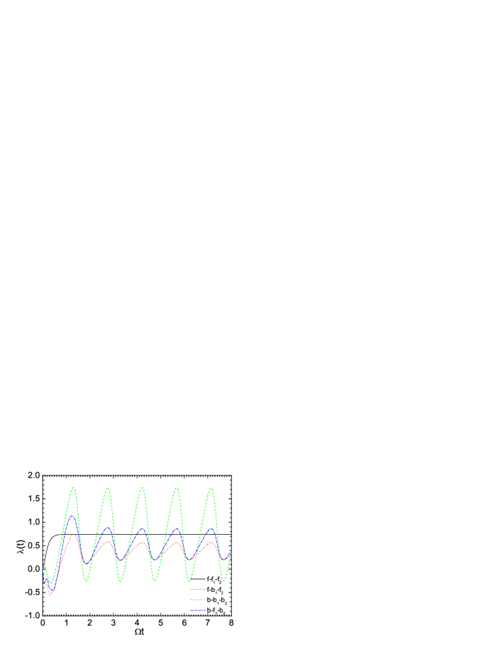
Because the friction coefficient $\lambda_{\scriptstyle b}(t)$ does not converge to a stationary value at $t\to+\infty$ (Fig. 1) Lac15 ; PRE18 , an asymptotic stationary value of occupation number $n_{\scriptstyle a}$ in Eq. (13) can be reached if the condition

$\displaystyle\frac{1}{p}\sum_{\lambda=1}^{N_{\bar{\scriptstyle a}}}I_{\bar{\scriptstyle a}_{\scriptscriptstyle\lambda}}(\infty)=\frac{\frac{1}{1-p}\sum_{\lambda=N_{\bar{\scriptstyle a}}+1}^{N}I_{{\scriptstyle a}_{\scriptscriptstyle\lambda}}(\infty)}{1+\frac{2{\varepsilon_{\scriptstyle a}}}{1-p}\sum_{\lambda=N_{\bar{\scriptstyle a}}+1}^{N}I_{{\scriptstyle a}_{\scriptscriptstyle\lambda}}(\infty)}$ (18)

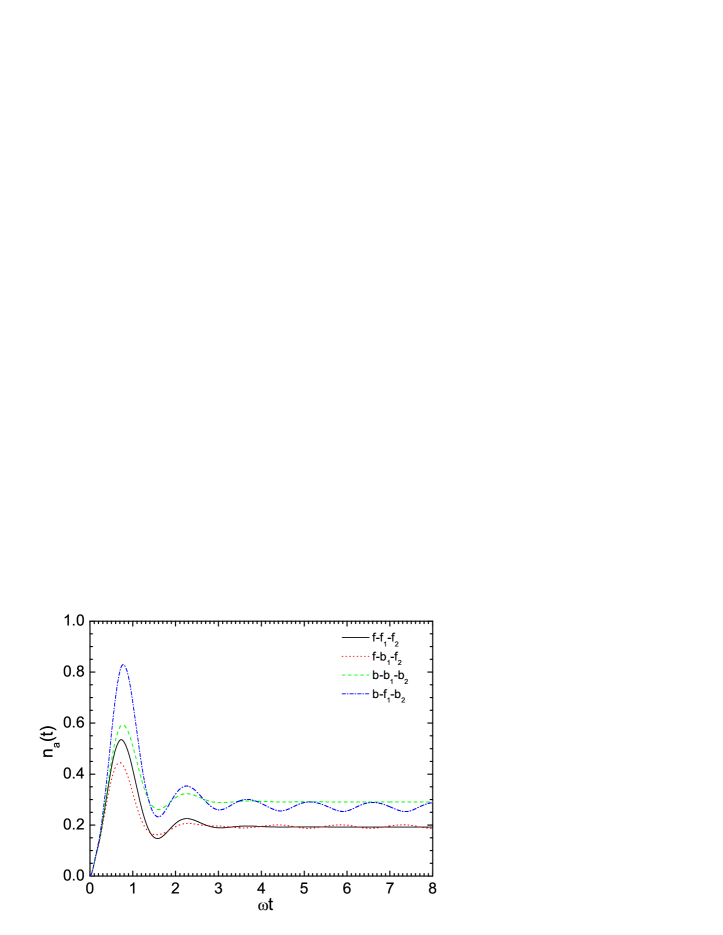
is satisfied PhysicaA2019 ; PRE2020 . In other cases, the occupation number remains oscillating at large time (Fig. 2) because the friction $\lambda_{\scriptscriptstyle b}(t)$ and, correspondingly, diffusion coefficient oscillate as a function of time (Fig. 1) Lac15 ; PRE18 . To obtain Eq. (18), the relation $D_{{\scriptstyle a}_{\scriptscriptstyle\lambda}}=\lambda_{\scriptstyle a}I_{{\scriptstyle a}_{\scriptscriptstyle\lambda}}$ is used at large time ($\Omega t\gg 1$).

The physical problem discussed here is considerably simplified when the $N$ baths have the same quantum nature. Then, the asymptotic occupation number is always stationary (Fig. 2) and given by

$\displaystyle n_{\scriptstyle a}(\infty)=\lim_{t\rightarrow\infty}\frac{D(t)}{\lambda(t)}=\lim_{t\rightarrow\infty}\frac{\sum_{\lambda=1}^{N}D_{{\scriptstyle a}_{\lambda}}(t)}{\lambda_{\scriptstyle a}(t)}=\sum_{\lambda=1}^{N}I_{{\scriptstyle a}_{\scriptscriptstyle\lambda}}(\infty)=I_{\scriptstyle a}(\infty)$ (19)

in the case when all reservoirs and system oscillator have the same quantum nature [$p=0$, $N_{\bar{\scriptstyle a}}=0$, $N_{\scriptstyle a}=N$] or

$\displaystyle n_{\scriptstyle a}(\infty)=\frac{\sum_{\lambda=1}^{N_{\bar{\scriptstyle a}}}I_{\bar{\scriptstyle a}_{\scriptscriptstyle\lambda}}(\infty)}{1-2{\varepsilon_{\scriptstyle a}}\sum_{\lambda=1}^{N_{\bar{\scriptstyle a}}}I_{\bar{\scriptstyle a}_{\scriptscriptstyle\lambda}}(\infty)}=\frac{I_{\bar{\scriptstyle a}}(\infty)}{1-2{\varepsilon_{\scriptstyle a}}I_{\bar{\scriptstyle a}}(\infty)}$ (20)

in the case when all reservoirs have the same quantum nature (${\bar{a}}={b}$ or $f$) which differs from the one of the system oscillator (${a}={f}$ or $b$) [$1-p=0$, $N_{\bar{\scriptstyle a}}=N$, $N_{\scriptstyle a}=0$]. Equations (19) and (20) generalize the equations given in Ref. PhysicaA for a single bath. If the baths have the same temperatures, then the asymptotic occupation number differs in general from the Fermi-Dirac or Bose-Einstein occupation number. Only in the Markovian weak-coupling limit and in the case of the same temperature $T_{\lambda}=T$ of all baths, Eqs. (19) and (20) are reduced to the usual Bose-Einstein and Fermi-Dirac thermal distributions $n_{\scriptstyle a}(\infty)=[\exp(\hbar\omega/kT)-{\varepsilon_{\scriptstyle a}}]^{-1}$ and the system has a thermal equilibrium.

Refer to caption
Refer to caption
Figure 1: The calculated dependencies of the friction and diffusion coefficients on time $t$ for the fermionic-fermionic-fermionic ($f-f_{1}-f_{2}$, solid line), bosonic-bosonic-bosonic ($b-b_{1}-b_{2}$, dashed line), the mixed fermionic-bosonic-fermionic ($f-b_{1}-f_{2}$, dotted line), and bosonic-fermionic-bosonic ($b-f_{1}-b_{2}$, dash-dotted line) systems.
Refer to caption
Figure 2: For the fermionic-fermionic-fermionic ($f-f_{1}-f_{2}$, solid line), bosonic-bosonic-bosonic ($b-b_{1}-b_{2}$, dashed line), the mixed fermionic-bosonic-fermionic ($f-b_{1}-f_{2}$, dotted line), and bosonic-fermionic-bosonic ($b-f_{1}-b_{2}$, dash-dotted line) systems, the calculated dependencies of the average occupation numbers on time $t$. The plots correspond to initially unoccupied, $n_{\text{a}}(t=0)$=0 system state.
Refer to caption
Figure 3: For the mixed fermionic-bosonic-fermionic ($f-b_{1}-f_{2}$), and bosonic-fermionic-bosonic ($b-f_{1}-b_{2}$) systems, the calculated dependence of the frequency of oscillations of $n_{\scriptstyle a}(t)$ at large $t$ on the oscillator renormalized frequency $\Omega$. For two systems, the results of calculations are coincide.

III Calculated results for fermionic or bosonic oscillator coupled with fermionic and bosonic baths in the case of Ohmic dissipation with Lorenzian cutoffs

In all figures of this paper presented for the fermionic or bosonic oscillator with two baths of the same or different statistics, we set $\gamma_{1}/\Omega=10$, $\gamma_{2}/\Omega=15$, $\alpha_{1}=0.1$, $\alpha_{2}=0.05$, $g_{0}=\alpha_{1}+\alpha_{2}=0.15$, $kT_{1}/(\hbar\Omega)=1$, and $kT_{2}/(\hbar\Omega)=0.1$. The values of $\gamma_{1,2}/\Omega$ are taken to hold the conditions $\gamma_{1,2}\gg\Omega$: the non-Markovian quantum Langevin approach can be applied when the system is slow in comparison to the relaxation times of the heat baths. The occupation numbers, diffusion and friction coefficients depend on the values of oscillator frequency $\omega$, coupling strengths $\alpha_{1}$, $\alpha_{2}$, inverse memory times $\gamma_{1,2}$, and heat bath temperatures $T_{1,2}$ (see Appendix A). A zero chemical potential is assumed here. The values of $\alpha_{1}$ and $\alpha_{2}$ are chosen to have the realistic values of friction coefficients which are known from the microscopic calculations. Indeed, these coupling strengths provide almost the same friction coefficient for relative motion of two nuclei like in Refs.Β Wash1 . As an example of bosonic system, the atomic or nuclear molecular state can be considered. The bound or quasi-bound particle (electron in the trap or nucleon in the isomeric state) can be taken as an example of fermionic system. The electromagnetic and temperature fields or phonon bath can be treated as the bosonic baths. Free electrons and inclusion in the compound can act as the fermionic baths.
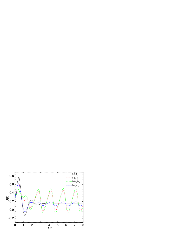
For the fermionic-fermionic-fermionic ($f-f_{1}-f_{2}$), bosonic-bosonic-bosonic ($b-b_{1}-b_{2}$), the mixed fermionic-bosonic-fermionic ($f-b_{1}-f_{2}$), and bosonic-fermionic-bosonic ($b-f_{1}-b_{2}$) systems, the time-dependent friction and diffusion coefficients are shown in Fig. 1. The diffusion and friction coefficients are equal to zero at initial time. As seen, the time dependencies of these coefficients are not the same for the different systems. For the $f-f_{1}-f_{2}$ system, the friction and diffusion coefficients relatively fast reach their asymptotic values (the transient time for the friction is quite short, $\Omega t\leq 0.5$), whereas in the case of $b-b_{1}-b_{2}$ and mixed $f-b_{1}-f_{2}$, $b-f_{1}-b_{2}$ systems they oscillate with the same period of oscillations. The amplitudes of oscillations for the system with two bosonic baths are larger than those for the systems with one bosonic bath. For the $b-b_{1}-b_{2}$ system, the friction and diffusion coefficients oscillate in the phase and, as a result, the occupation number has asymptotic limit (Fig. 2). In the contrast, for the mixed systems $f-b_{1}-f_{2}$ and $b-f_{1}-b_{2}$, the occupation number oscillates around certain average value at large times, so it has no asymptotic limit. For both systems, the periods of oscillations are the same. The occupation number for the fermionic oscillator oscillates with the larger amplitude than one for the bosonic oscillator (Fig. 2). The absolute value of oscillations mainly depend on the coupling constants. The times to reach the asymptotic oscillations are almost the same for these systems.

In the case when fermionic bath coexists with bosonic bath, at large times the influence of the thermostats is minimal and reversible - it takes energy from the system and gives the same amount of energy back. As a result, the population of the excited state(s) decreases and then increases on the same level independent of the environment. As shown in Fig. 3, the period of oscillations of $n_{\scriptstyle a}(t)$ at large $t$ depends on the frequency of oscillator and, accordingly, carries information about the system. At $\Omega/\gamma_{1}>0.1$, the frequency of asymptotic oscillations is proportional to the oscillator frequency. Since the asymptotic oscillations of the occupation number depend on the oscillator frequency, this gives a new opportunity to control these oscillations by changing the oscillator frequency. For example, by this way one can control the amplification or attenuation of signal transmission. Since the asymptotic oscillations are independent of the medium, one can unambiguously judge the population of the excited state of two-level system, which, for example, is important in quantum computers. In this case, it is necessary to ensure a sufficient degree of metastability of the excited states of the quantum register. These states must have sufficiently a large lifetime that determines their relaxation to the ground state due to dissipative processes. Such a system with non-stationary asymptotics can be used as a dynamic (non-stationary) memory system because the information about some properties of the system (population of excitation state(s) and frequency) is preserved at large times. So, we suggest to store information by using the non-stationary memory systems. This idea can be effective, because such systems will be stable under external conditions.

IV Conclusions

In conclusion, for the bosonic or fermionic oscillator fully coupled with the mixed bosonic-fermionic heat baths, the absence of equilibrium asymptotic of occupation number was predicted. At large times, the period of oscillations of occupation number depends on the frequency of oscillator and, accordingly, carries information about the system. It is an example of nonstationary (dynamic) memory storage. Each frequency corresponds to certain state and can lead to the control of these states for recording data in quantum computers and increasing channels and speeds of communication. As shown, this behavior is also expected for other non-stationary systems (not necessarily an oscillator fully coupled with several fermionic and bosonic heat baths) in which the asymptotic friction $\lambda(t)$ and diffusion $D(t)$ coefficients periodically oscillate out of phase.

Acknowledgments

G.G.A. and N.V.A. were supported by Ministry of Science and Higher Education of the Russian Federation (Moscow, Contract No. 075-10-2020-117). V.V.S. acknowledges the Alexander von Humboldt-Stiftung (Bonn). D.L. thanks the CNRS for financial support through the 80Prime program. This work was partly supported by the IN2P3(France)-JINR(Dubna) Cooperation Programme and DFG (Bonn, Grant No. Le439/16).

Appendix A Explicit expressions for friction and diffusion coefficients of fermionic (bosonic) oscillator with several fermionic (bosonic) heat baths

Let us consider the case when all $N$ heat baths and system oscillator with the frequency $\omega$ are either all bosonic or all fermionic. For these systems, the details of the procedure for obtaining the occupation number of system are given in Ref. PRE18 . Here, we directly write the final expression for the time dependence of occupation number:

$$\begin{split}n_{{\scriptstyle a}}(t)=n_{{\scriptstyle a}}(0)|A(t)|^{2}+[1+\varepsilon_{{\scriptstyle a}}n_{{{\scriptstyle a}}}(0)]|B(t)|^{2}+I_{{\scriptstyle a}}(t),\end{split}$$ (21)

where $I_{{\scriptstyle a}}(t)=\sum_{\lambda}I_{{{\scriptstyle a}}_{\scriptscriptstyle\lambda}}(t)$ and

$\displaystyle I_{{{\scriptstyle a}}_{\scriptscriptstyle\lambda}}(t)=\frac{\alpha_{\scriptstyle\lambda}\gamma_{\scriptstyle\lambda}^{2}}{\pi}\int_{0}^{\infty}dw\frac{w}{\gamma_{\scriptstyle\lambda}^{2}+w^{2}}\left[n^{({\scriptstyle\lambda})}(w)|M(w,t)|^{2}+[1+\varepsilon_{\scriptstyle\lambda}n^{({\scriptstyle\lambda})}(w)]|N(w,t)|^{2}\right],$ (22)
A​(t)=12β€‹βˆ‘k=1N0ΞΎk​esk​t​(skβˆ’s0)Γ—{2​skβˆ’i​[Ξ©+Ο‰]βˆ’2​i​skβ€‹βˆ‘Ξ»=1Nαλ​γλsk+Ξ³Ξ»}β€‹βˆΞΌ=1N(sk+Ξ³ΞΌ)=iβ€‹βˆ‘Ξ»=1Nαλ​γλ2β€‹βˆ‘k=1N0ΞΎk​esk​t​(skβˆ’s0)​skβˆ’i​ωsk+iβ€‹Ο‰β€‹βˆΞΌ=1,ΞΌβ‰ Ξ»N(sk+Ξ³ΞΌ),B​(t)=i2β€‹βˆ‘k=1N0ΞΎk​esk​t​(skβˆ’s0)Γ—{Ξ©βˆ’Ο‰+2​skβ€‹βˆ‘Ξ»=1Nαλ​γλsk+Ξ³Ξ»}β€‹βˆΞΌ=1N(sk+Ξ³ΞΌ)=iβ€‹βˆ‘Ξ»=1Nαλ​γλ2β€‹βˆ‘k=1N0ΞΎk​esk​t​(s0βˆ’sk)β€‹βˆΞΌ=1,ΞΌβ‰ Ξ»N(sk+Ξ³ΞΌ),N​(w,t)=βˆ‘k=0N0ΞΎk​esk​t​(i​skβˆ’Ο‰)β€‹βˆΞΌ=1N(sk+Ξ³ΞΌ),M​(w,t)=βˆ’βˆ‘k=0N0ΞΎk​esk​t​(i​sk+Ο‰)β€‹βˆΞΌ=1N(sk+Ξ³ΞΌ),formulae-sequence𝐴𝑑12superscriptsubscriptπ‘˜1subscript𝑁0subscriptπœ‰π‘˜superscript𝑒subscriptπ‘ π‘˜π‘‘subscriptπ‘ π‘˜subscript𝑠02subscriptπ‘ π‘˜π‘–delimited-[]Ξ©πœ”2𝑖subscriptπ‘ π‘˜superscriptsubscriptπœ†1𝑁subscriptπ›Όπœ†subscriptπ›Ύπœ†subscriptπ‘ π‘˜subscriptπ›Ύπœ†superscriptsubscriptproductπœ‡1𝑁subscriptπ‘ π‘˜subscriptπ›Ύπœ‡π‘–superscriptsubscriptπœ†1𝑁subscriptπ›Όπœ†subscriptsuperscript𝛾2πœ†superscriptsubscriptπ‘˜1subscript𝑁0subscriptπœ‰π‘˜superscript𝑒subscriptπ‘ π‘˜π‘‘subscriptπ‘ π‘˜subscript𝑠0subscriptπ‘ π‘˜π‘–πœ”subscriptπ‘ π‘˜π‘–πœ”superscriptsubscriptproductformulae-sequenceπœ‡1πœ‡πœ†π‘subscriptπ‘ π‘˜subscriptπ›Ύπœ‡π΅π‘‘π‘–2superscriptsubscriptπ‘˜1subscript𝑁0subscriptπœ‰π‘˜superscript𝑒subscriptπ‘ π‘˜π‘‘subscriptπ‘ π‘˜subscript𝑠0Ξ©πœ”2subscriptπ‘ π‘˜superscriptsubscriptπœ†1𝑁subscriptπ›Όπœ†subscriptπ›Ύπœ†subscriptπ‘ π‘˜subscriptπ›Ύπœ†superscriptsubscriptproductπœ‡1𝑁subscriptπ‘ π‘˜subscriptπ›Ύπœ‡π‘–superscriptsubscriptπœ†1𝑁subscriptπ›Όπœ†subscriptsuperscript𝛾2πœ†superscriptsubscriptπ‘˜1subscript𝑁0subscriptπœ‰π‘˜superscript𝑒subscriptπ‘ π‘˜π‘‘subscript𝑠0subscriptπ‘ π‘˜superscriptsubscriptproductformulae-sequenceπœ‡1πœ‡πœ†π‘subscriptπ‘ π‘˜subscriptπ›Ύπœ‡formulae-sequence𝑁𝑀𝑑superscriptsubscriptπ‘˜0subscript𝑁0subscriptπœ‰π‘˜superscript𝑒subscriptπ‘ π‘˜π‘‘π‘–subscriptπ‘ π‘˜πœ”superscriptsubscriptproductπœ‡1𝑁subscriptπ‘ π‘˜subscriptπ›Ύπœ‡π‘€π‘€π‘‘superscriptsubscriptπ‘˜0subscript𝑁0subscriptπœ‰π‘˜superscript𝑒subscriptπ‘ π‘˜π‘‘π‘–subscriptπ‘ π‘˜πœ”superscriptsubscriptproductπœ‡1𝑁subscriptπ‘ π‘˜subscriptπ›Ύπœ‡\begin{split}A(t)&=\frac{1}{2}\sum_{k=1}^{N_{0}}\xi_{k}e^{s_{k}t}(s_{k}-s_{0})\\ &\times\left\{2s_{k}-i[\Omega+\omega]-2is_{k}\sum_{\lambda=1}^{N}\frac{\alpha_{\scriptstyle\lambda}\gamma_{\scriptstyle\lambda}}{s_{k}+\gamma_{\scriptstyle\lambda}}\right\}\prod_{\mu=1}^{N}(s_{k}+\gamma_{\scriptstyle\mu})\\ &=i\sum_{\lambda=1}^{N}\alpha_{\scriptstyle\lambda}\gamma^{2}_{\scriptstyle\lambda}\sum_{k=1}^{N_{0}}\xi_{k}e^{s_{k}t}(s_{k}-s_{0})\frac{s_{k}-i\omega}{s_{k}+i\omega}\prod_{\mu=1,\mu\neq\lambda}^{N}(s_{k}+\gamma_{\scriptstyle\mu}),\\ B(t)&=\frac{i}{2}\sum_{k=1}^{N_{0}}\xi_{k}e^{s_{k}t}(s_{k}-s_{0})\\ &\times\left\{\Omega-\omega+2s_{k}\sum_{\lambda=1}^{N}\frac{\alpha_{\scriptstyle\lambda}\gamma_{\scriptstyle\lambda}}{s_{k}+\gamma_{\scriptstyle\lambda}}\right\}\prod_{\mu=1}^{N}(s_{k}+\gamma_{\scriptstyle\mu})\\ &=i\sum_{\lambda=1}^{N}\alpha_{\scriptstyle\lambda}\gamma^{2}_{\scriptstyle\lambda}\sum_{k=1}^{N_{0}}\xi_{k}e^{s_{k}t}(s_{0}-s_{k})\prod_{\mu=1,\mu\neq\lambda}^{N}(s_{k}+\gamma_{\scriptstyle\mu}),\\ N(w,t)&=\sum_{k=0}^{N_{0}}\xi_{k}e^{s_{k}t}(is_{k}-\omega)\prod_{\mu=1}^{N}(s_{k}+\gamma_{\scriptstyle\mu}),\\ M(w,t)&=-\sum_{k=0}^{N_{0}}\xi_{k}e^{s_{k}t}(is_{k}+\omega)\prod_{\mu=1}^{N}(s_{k}+\gamma_{\scriptstyle\mu}),\end{split} (23)

where

ΞΎk=∏i=0,iβ‰ kN01skβˆ’sisubscriptπœ‰π‘˜superscriptsubscriptproductformulae-sequence𝑖0π‘–π‘˜subscript𝑁01subscriptπ‘ π‘˜subscript𝑠𝑖\xi_{k}=\prod_{i=0,\\ i\neq k}^{N_{0}}\frac{1}{s_{k}-s_{i}} (24)

with $s_{0}=-iw$ and the roots sksubscriptπ‘ π‘˜s_{k}, $k=1,...,N_{0}$, of the $N_{0}=N+2$ order polynomial:

[s2+Ο‰2βˆ’2β€‹Ο‰β€‹βˆ‘Ξ»=1Nαλ​γλ2s+Ξ³Ξ»]β€‹βˆΞΌ=1N(s+Ξ³ΞΌ)=0.delimited-[]superscript𝑠2superscriptπœ”22πœ”superscriptsubscriptπœ†1𝑁subscriptπ›Όπœ†subscriptsuperscript𝛾2πœ†π‘ subscriptπ›Ύπœ†superscriptsubscriptproductπœ‡1𝑁𝑠subscriptπ›Ύπœ‡0\displaystyle\left[s^{2}+\omega^{2}-2\omega\sum_{\lambda=1}^{N}\frac{\alpha_{\scriptstyle\lambda}\gamma^{2}_{\scriptstyle\lambda}}{s+\gamma_{\scriptstyle\lambda}}\right]\prod_{\mu=1}^{N}(s+\gamma_{\scriptstyle\mu})=0. (25)

Here,

$\displaystyle\Omega=\omega-2\sum_{\lambda=1}^{N}\alpha_{\scriptstyle\lambda}\gamma_{\scriptstyle\lambda}$ (26)

is the renormalized frequency and $\varepsilon_{\scriptstyle\lambda}$ is equal to 1 (-1) for the bosonic (fermionic) heat bath β€Ξ»πœ†\lambda”.

In Eq. (22), $n^{({\scriptstyle\lambda})}(w)=(\exp[\hbar w/(kT_{{\scriptstyle\lambda}})]-\varepsilon_{\scriptstyle\lambda})^{-1}$ is equilibrium Fermi-Dirac (Bose-Einstein) distribution of the fermionic (bosonic) heat bath β€Ξ»πœ†\lambda”. The $T_{{\scriptstyle\lambda}}$ is the initial thermodynamic temperature of the corresponding heat bath. Here, we introduce the spectral density $\rho_{\scriptstyle\lambda}(w)$ of the heat-bath excitations, which allows us to replace the sum over $i$ by integral over the frequency $w$: $\sum_{i}...\to\int_{0}^{\infty}dw\rho_{\scriptstyle\lambda}(w)...$. For all baths, we consider the following spectral function M1 :

$\displaystyle\dfrac{\alpha_{\scriptstyle{\lambda,i}}^{2}}{\hbar^{2}w_{\scriptstyle{\lambda,i}}}\to\dfrac{\rho_{\scriptstyle\lambda}(w)\alpha_{\scriptstyle{\lambda,w}}^{2}}{\hbar^{2}w}=\dfrac{1}{\pi}\alpha_{\scriptstyle\lambda}\dfrac{\gamma_{{\scriptstyle\lambda}}^{2}}{\gamma_{{\scriptstyle\lambda}}^{2}+w^{2}},$ (27)

where the memory time $\gamma_{{\scriptstyle\lambda}}^{-1}$ of dissipation is inverse to the bandwidth of the heat-bath excitations which are coupled to the collective system. This is the Ohmic dissipation with the Lorenzian cutoff (Drude dissipation). The relaxation time of the heat-bath should be much less than the characteristic collective time. The similarity of expressions for the occupation numbers for fermionic and bosonic systems results from the similarity of the equations of motion for creation and annihilation operators Lac15 ; Lac16 .

Making derivative of Eq. (21) in $t$ and simple but tedious algebra, we derive the following differential equation for the occupation number:

$$\frac{dn_{\scriptstyle a}(t)}{dt}=-2\lambda_{\scriptstyle a}(t)n_{\scriptstyle a}(t)+2D_{\scriptstyle a}(t),$$ (28)

where

$$\lambda_{\scriptstyle a}(t)=-\frac{1}{2}\frac{d}{dt}\ln\left[|A(t)|+\varepsilon_{\scriptstyle a}|B(t)|^{2}\right]$$ (29)

and

$\displaystyle D_{\scriptstyle a}(t)$ $\displaystyle=$ $\displaystyle\sum_{\lambda=1}^{N}D_{{\scriptstyle a}_{\scriptscriptstyle\lambda}}(t)=\lambda_{\scriptstyle a}(t)\big{[}|B(t)|^{2}+I_{\scriptstyle a}(t)\big{]}+\frac{1}{2}\frac{d}{dt}\big{[}|B(t)|^{2}+I_{\scriptstyle a}(t)\big{]},$
$\displaystyle D_{{\scriptstyle a}_{\scriptscriptstyle\lambda}}(t)$ $\displaystyle=$ $\displaystyle\lambda_{\scriptstyle a}(t)\big{[}J_{\scriptstyle\lambda}(t)+I_{{\scriptstyle a}_{\scriptscriptstyle\lambda}}(t)\big{]}+\frac{1}{2}\frac{d}{dt}\big{[}J_{\scriptstyle\lambda}(t)+I_{{\scriptstyle a}_{\scriptscriptstyle\lambda}}(t)\big{]}$ (30)

are the time-dependent friction and diffusion coefficients, respectively. The following decomposition $|B(t)|^{2}=\sum_{\lambda}J_{\scriptstyle\lambda}(t)$ is used in Eq. (A). Here, $\lambda_{\scriptstyle a}(t=0)=D_{\text{a}}(t=0)=0$. Therefore, we have obtained the equation for $n_{\scriptstyle a}(t)$ which is local in time. In the case of constant transport coefficients, this equation describes the Markovian dynamics, i.e. the evolution of $n_{\scriptstyle a}(t)$ is independent of the past. In Eq.Β (28), the transport coefficients explicitly depend on time and the non-Markovian effects are taken into consideration through this time dependence PRE18 . The non-Markovian feature of Eq.Β (28) is well seen at $D_{\scriptstyle a}=0$. In this case, $n_{\scriptstyle a}(t)\sim\exp\left(-2\int_{0}^{t}\lambda_{\scriptstyle a}(t)dt\right)$, i.e. the occupation number depends on the time dependence of $\lambda_{\scriptstyle a}$. Because $A(\infty)=B(\infty)=0$ PRE18 , the appropriate asymptotic equilibrium distribution

$\displaystyle n_{\scriptstyle a}(\infty)=\frac{D_{\scriptstyle a}(\infty)}{\lambda_{\scriptstyle a}(\infty)}=\sum_{\lambda}I_{{\scriptstyle a}_{\scriptscriptstyle\lambda}}(\infty)$ (31)

is achieved [see Eqs.(21) and (28)]. Using Eqs.Β (A1) and (A2), the asymptotic values of $|M(w,t)|^{2}$ and $|N(w,t)|^{2}$ are found. With these values we obtain from (22)

$\displaystyle I_{{\scriptstyle a}_{\scriptscriptstyle\lambda}}(t\to\infty)$ $\displaystyle=$ $\displaystyle\frac{\alpha_{\scriptstyle\lambda}\gamma_{\scriptstyle\lambda}^{2}}{\pi}\int_{0}^{\infty}dw\frac{w}{\gamma_{\scriptstyle\lambda}^{2}+w^{2}}\left\{[\omega+w]^{2}n^{({\scriptstyle\lambda})}(w)+[\omega-w]^{2}[1+\varepsilon_{\scriptstyle\lambda}n^{({\scriptstyle\lambda})}(w)]\right\}$ (32)
$\displaystyle\times$ ∏μ=1Nb(Ξ³ΞΌ2+w2)∏k=1N0(sk2+w2).superscriptsubscriptproductπœ‡1subscript𝑁𝑏superscriptsubscriptπ›Ύπœ‡2superscript𝑀2superscriptsubscriptproductπ‘˜1subscript𝑁0superscriptsubscriptπ‘ π‘˜2superscript𝑀2\displaystyle\frac{\prod_{\mu=1}^{N_{b}}(\gamma_{\scriptstyle\mu}^{2}+w^{2})}{\prod_{k=1}^{N_{0}}(s_{k}^{2}+w^{2})}.

The specific quantum nature of the baths enters into the diffusion coefficient through the appearance of occupation probabilities. The asymptotic diffusion and friction coefficients are related by the well-known fluctuation-dissipation relations connecting diffusion and damping constants. Fulfillment of the fluctuation-dissipation relations means that we have correctly defined the dissipative kernels in the non-Markovian equations of motion. In the Markovian limit (weak-couplings and high temperatures), the asymptotic occupation number is:

$$n_{\scriptstyle a}(\infty)=\frac{1}{g_{0}}\sum_{\lambda}\alpha_{\scriptstyle\lambda}n^{({\scriptstyle\lambda})}(\omega),$$

where $g_{0}=\sum_{\lambda}\alpha_{\scriptstyle\lambda}$.

References

  • (1) E. Stefanescu and W. Scheid, Physica A 374, 203 (2007); E. Stefanescu, W. Scheid, and A. Sandulescu, Ann. Phys. 323, 1168 (2008); E. Stefanescu, Prog. Quant. Electr. 34, 349 (2010).
  • (2) L. Lamata, D.R. Leibrandt, I. L. Chuang, J. I. Cirac, M.D. Lukin, V. VuletiΔ‡, and S. F. Yelin, Phys. Rev. Lett. 107, 030501 (2011).
  • (3) G.-D. Lin and L.-M. Duan, New J. Phys. 13, 075015 (2011).
  • (4) A. Nunnenkamp, J. Koch, and S.M. Girvin, New J. Phys. 13, 095008 (2011).
  • (5) A. Majumdar, D. Englund, M. Bajcsy, and J. VuckoviΔ‡, Phys. Rev. A 85, 033802 (2012).
  • (6) S.D. Bennett, N.Y. Yao, J. Otterbach, P. Zoller, P. Rabl, and M.D. Lukin, Phys. Rev. Lett. 110, 156402 (2013).
  • (7) M. Chen and J.Q. You, Phys. Rev. A 87, 052108 (2013); C.-K. Chan, G.-D. Lin, S.F. Yelin, and M.D. Lukin, Phys. Rev. A 89, 042117 (2014).
  • (8) A.A. Hovhannisyan, V.V. Sargsyan, G.G. Adamian, N.V. Antonenko, and D. Lacroix, Phys. Rev. E 97, 032134 (2018).
  • (9) M. Mwalaba, I. Sinayskiy, and F. Petruccione, Phys. Rev. A 99, 052102 (2019).
  • (10) D. Lacroix, V.V. Sargsyan, G.G. Adamian, N.V. Antonenko, and A.A. Hovhannisyan, Phys. Rev. A 102, 022209 (2020).
  • (11) A.A. Hovhannisyan, V.V. Sargsyan, G.G. Adamian, N.V. Antonenko, and D. Lacroix, Physica A 545, 123653 (2020).
  • (12) A.A. Hovhannisyan, V.V. Sargsyan, G.G. Adamian, N.V. Antonenko, and D. Lacroix, Phys. Rev. E 101, 062115 (2020).
  • (13) K. Lindenberg and B. J. West, The Nonequilibrium Statistical Mechanics of Open and Closed Systems (VCH Publishers, Inc., New York, 1990); K. Lindenberg and B. J. West, Phys. Rev. A 30, 568 (1984).
  • (14) F. Haake and R. Reibold, Phys. Rev. A 32, 2462 (1985).
  • (15) V. V. Dodonov and V. I. Man’ko, Density Matrices and Wigner Functions of Quasiclassical Quantum Systems (Proc. Lebedev Phys. Inst. of Sciences, Vol. 167, A. A. Komar, ed.), Nova Science, Commack, N. Y. (1987).
  • (16) A. Isar, A. Sandulescu, H. Scutaru, E. Stefanescu, and W. Scheid, Int. J. Mod. Phys. E 3, 635 (1994).
  • (17) Th.M. Nieuwenhuizen and A.E. Allahverdyan, Phys. Rev. E 66, 036102 (2002).
  • (18) V.V. Sargsyan, A.A. Hovhannisyan, G.G. Adamian, N.V. Antonenko, and D. Lacroix, Physica A 505, 666 (2018).
  • (19) V.V. Sargsyan, D. Lacroix, G.G. Adamian, and N.V. Antonenko, Phys. Rev. A 95, 032119 (2017).
  • (20) V.V. Sargsyan, D. Lacroix, G.G. Adamian, and N.V. Antonenko, Phys. Rev. A 90, 022123 (2014); 96, 012114 (2017).
  • (21) K.Β Washiyama and D.Β Lacroix, Phys. Rev. C 78, 024610 (2008); K.Β Washiyama, D.Β Lacroix, and S.Β Ayik, Phys. Rev. C 79, 024609 (2009).