Finite-temperature magnetic properties of Sm₂Fe₁₇N_x
using an ab-initio effective spin model

Abstract

In this study, we investigate the finite-temperature magnetic properties of Sm₂Fe₁₇N_x ($x=0,3$) using an effective spin model constructed based on the information obtained by first-principles calculations. We find that assuming the plausible trivalent Sm³⁺ configuration results in a model that can satisfactorily describe the magnetization curves of Sm₂Fe₁₇N₃. By contrast, the model based on the divalent Sm²⁺ configuration is suitable to reproduce the magnetization curves of Sm₂Fe₁₇. These results expand the understanding of how electronic structure affects the magnetic properties of these compounds.

I Introduction

The Sm₂Fe₁₇N_x nitrides have unusual magnetic anisotropy properties. The system with $x=3$ is a commercially successful permanent magnet and is well known to exhibit stronger uniaxial magnetocrystalline anisotropy than Nd₂Fe₁₄B. In contrast, the system with $x=0$, binary Sm₂Fe₁₇, has weak planar anisotropy, and a recent experiment has revealed that the magnetization orientation slightly deviates from the basal plane by about 10$\tcdegree$ at low temperatures diop . Because the iron sublattice of this system is expected to have planar magnetic anisotropy analogous to Y₂Fe₁₇, this observation indicates that the local magnetic anisotropy due to the Sm ions is uniaxial but comparatively weak in Sm₂Fe₁₇. Thus, the nitrogenation process sensitively changes the electronic states around the Sm ions, resulting in a sign change of the magnetocrystalline anisotropy.

Several efforts have been made to theoretically clarify the electronic states of Sm₂Fe₁₇N_x based on first-principles calculations min ; steinbeck ; nekrasov ; pandey ; ogura . Because modern first-principles calculations still do not treat 4f electrons properly, some additional treatment such as the so-called open core method, the local spin density approximation with Hubbard correction (LSDA+$U$), or the self-interaction correction (SIC) is needed to evaluate the magnetic anisotropy of these systems. Steinbeck et al. steinbeck calculated the 4f crystal field parameters (CFPs) for the Sm ions based on the open core method, assuming a plausible trivalent Sm³⁺ configuration. They found that the second-order CFP $A_{2}^{0}$, which dominates the local magnetic anisotropy of Sm, is enhanced in amplitude by nitrogenation. Knyazev et al. nekrasov calculated the electronic structure and optical properties of Sm₂Fe₁₇ and Tm₂Fe₁₇ using the LSDA+$U$ method. The calculated total magnetic moment including the orbital correction to the contribution from 4f electrons is in good agreement with the experimentally measured valueKou . However, they did not discuss the magnetic anisotropy of the systems. Pandey et al. pandey calculated the magnetocrystalline anisotropy energy of Sm₂Fe₁₇ and Sm₂Fe₁₇N₃. The predicted directions of magnetocrystalline anisotropy for Sm₂Fe₁₇ and Sm₂Fe₁₇N₃ are in good agreement with the experimental observations. However, the calculated total moments are smaller than the experimentally measured valuesBuschow ; McNeely . According to their results, the calculated spin magnetic moments of the Sm ions are close to that of trivalent Sm³⁺. Recently, Ogura et al. ogura carried out self-consistent Korringa–Kohn–Rostoker coherent potential approximation (KKR-CPA) calculations with a SIC treatment, and confirmed that the uniaxial magnetocrystalline anisotropy increases with increasing nitrogen content $x$. In addition, they claimed that the number of f electrons of each Sm ion is about 6; that is, a divalent Sm²⁺ configuration is realized, regardless of $x$. This result is quite intriguing because it has been widely believed that the Sm ions have trivalent electronic states, as claimed in several X-ray absorption spectroscopy (XAS) experimentsXAS .

We notice that these theoretical studies except the work of Pandey et al. concluded uniaxial magnetocrystalline anisotropy not only for Sm₂Fe₁₇N₃, but also for Sm₂Fe₁₇, which is inconsistent with the reported experimental observations. It should be also noted here that the KKR-CPA with SIC calculations showed that the uniaxial magnetic anisotropy of Sm₂Fe₁₇ is fairly small. This is intuitively understandable because the 4f electron clouds of divalent Sm²⁺ should be more spherical than those of trivalent Sm³⁺, resulting in a weaker uniaxial local magnetic anisotropy. Although information about the electronic states of Sm is quite important to understand the magnetic properties, in particular, the magnetocrystalline anisotropy, it is difficult to extend the conclusions of the previous studies by using the first-principles calculation method itself. Therefore, we instead focus on the finite-temperature magnetic properties of the systems. We construct a single-ion model, which has long been used to describe phenomenologically the magnetic properties of rare-earth based materials, but base it on first-principles calculations. The necessary information to construct the model is as follows: the magnetic moments of each ion, the exchange field acting on the 4f electrons, and the CFPs. Once we construct the model, including the crystal-field Hamiltonian, we can compute the magnetic anisotropy due to the rare-earth ions for arbitrary temperatures in the standard statistical mechanical way. For this purpose, the most suitable way to treat the 4f electrons in first-principles calculations is the open core method because we can easily control the electronic structure and valency of the Sm ions.

In this study, we investigate the magnetization curves of Sm₂Fe₁₇N_x $(x=0,3)$ for several temperatures using the single-ion model based on first-principles calculations. We prepare the model in two ways: (1) assuming trivalent Sm ions, and (2) assuming divalent Sm ions. We show the differences between the magnetization curves obtained by (1) and (2), and discuss which valency and electronic configurations plausibly describe the experimentally obtained finite-temperature magnetic properties.

II Electronic structure calculations and model construction

We use the single-ion HamiltonianWijn ; Sankar ; Yamada ; Richter ; Franse to describe the finite-temperature magnetic properties of Sm₂Fe₁₇N_x $(x=0,3)$. The Hamiltonian of the $i$-th Sm ion is given as

$${\cal H}(i)$$

$$=\lambda{\bm{L}}_{\mathrm{4f}}{\bm{\cdot}}{\bm{S}}_{\mathrm{4f}}+2{\bm{H}}_{\textrm{m}}(T){\bm{\cdot}}{\bm{S}}_{\mathrm{4f}}+{\cal H}_{\mathrm{CEF}}(i)+\left({\bm{L}}_{\mathrm{4f}}+2{\bm{S}}_{\mathrm{4f}}\right){\bm{\cdot}}{\bm{H}}_{\mathrm{ex}},$$ (1)

where ${\bm{L}}_{\mathrm{4f}}$ and ${\bm{S}}_{\mathrm{4f}}$ are the total spin and total angular momentum operators, $\lambda$ is the spin-orbit coupling constant of the 4f shell, ${\bm{H}}_{\mathrm{ex}}$ is the external magnetic field, and ${\bm{H}}_{\textrm{m}}(T)$ is the exchange mean-field acting on the spin components of 4f electrons. The crystal-field Hamiltonian $H_{\textrm{CEF}}(i)$ is expressed in terms of the tensor operator method as followsSankar ; Yamada :

$$H_{\textrm{CEF}}(i)=A_{2}^{0}(i)\sum_{j}r^{2}_{j}2U_{2}^{0}(\theta_{j},\phi_{j})$$

$$+A_{4}^{0}(i)\sum_{j}r^{4}_{j}8U_{4}^{0}(\theta_{j},\phi_{j})+A_{6}^{0}(i)\sum_{j}r_{j}^{6}16U_{6}^{0}(\theta_{j},\phi_{j})$$

$$+A_{6}^{6}(i)\sum_{j}r_{j}^{6}16\left(\frac{1}{231}\right)^{\frac{1}{2}}\left[U_{6}^{6}(\theta_{j},\phi_{j})+U_{6}^{-6}(\theta_{j},\phi_{j})\right],$$ (2)

where $A_{l}^{m}(i)$ are the CFPs at the $i$-th rare-earth ion site. In this work, assuming that all sites are equivalent, we neglect contributions from $A_{4}^{3}(i)$ and $A_{6}^{3}(i)$. The tensor operator $U_{l}^{m}$ is given by

$$U_{l}^{m}(\theta_{j},\phi_{j})=\sqrt{\frac{4\pi}{2l+1}}Y_{l,m}(\theta_{j},\phi_{j}),$$ (3)

where $Y_{l,m}$ is the spherical harmonics function. Matrix elements of $\sum_{j}r^{l}_{j}U_{l}^{m}(\theta_{j},\phi_{j})$ are expressed using 3-j and 6-j symbols as followsSankar ; Yamada :

$$\langle J,J_{z},L,S|\sum_{j}r^{l}_{j}U_{l}^{m}(\theta_{j},\phi_{j})|J^{\prime},J^{\prime}_{z},L,S\rangle$$

$$=(-1)^{(L+S-J_{z}+J+J^{\prime})}\sqrt{(2J+1)(2J^{\prime}+1)}$$

$$\times\begin{pmatrix}J&J^{\prime}&l\\ -J_{z}&J^{\prime}_{z}&m\\ \end{pmatrix}\begin{Bmatrix}L&L&l\\ J&J^{\prime}&S\\ \end{Bmatrix}\langle L||U_{l}||L\rangle\langle r^{l}\rangle,$$ (4)

where $\langle L||U_{l}||L\rangle$ is the appropriate set of reduced matrix elements given in Table 1.

Table 1: The reduced matrix elements Yamada used in our calculations.

	$\langle L||U_{2}||L\rangle$	$\langle L||U_{4}||L\rangle$	$\langle L||U_{6}||L\rangle$
Sm3+	$\frac{1}{3}\left(\frac{2\cdot 11\cdot 13}{15}\right)^{\frac{1}{2}}$	$\frac{2}{3}(\frac{2\cdot 13}{11})^{\frac{1}{2}}$	$-10(\frac{5\cdot 17}{3\cdot 11\cdot 13})^{\frac{1}{2}}$
Sm2+	$2(\frac{7}{15})^{\frac{1}{2}}$	$-(\frac{14}{11})^{\frac{1}{2}}$	$10(\frac{7}{3\cdot 11\cdot 13})^{\frac{1}{2}}$

We note that $J$ multiplets are taken into account up to the fifth excited state in this calculation. We use $L=5$ and $S=\frac{5}{2}$ for Sm³⁺, and $L=3$ and $S=3$ for Sm²⁺.

Once we have set the Hamiltonian for the $i$-th Sm ion, we can obtain the free energy for the 4f partial system based on the statistical mechanical procedure, as

$$F(i)=-k_{\rm B}T\ln{\rm Tr}\exp\left[-\frac{{\cal H}(i)}{k_{\rm B}T}\right].$$ (5)

This single-ion Hamiltonian has a quite long history, and in the early days of the study of rare-earth-based permanent magnets, the model parameters such as $|{\bm{H}}_{\textrm{m}}(0)|$ and $A_{l}^{m}$ were determined by multi-parameter fitting calculations to the experimental magnetization curves of single crystals Yamada . Now, we can determine these parameters based on the information of the electronic states of the systems using first-principles calculations. Recently, we have confirmed that this procedure successfully describes the observed magnetization curves and the temperature dependences of anisotropy constants of R₂Fe₁₄B (R = Dy, Ho)Yoshiokasan and SmFe₁₂Yoshioka1-12 .

We use the first-principles calculations method to determine the CFPs. Once the electronic state calculations are completed, we can compute the CFPs $A_{l}^{m}\langle r^{l}\rangle$ in Eq. (II) based on the well-known formula Novak ; Divis1 ; Divis2

$$A_{l}^{m}\langle r^{l}\rangle=a_{lm}\int_{0}^{R_{\mathrm{MT}}}drr^{2}|R_{\rm 4f}(r)|^{2}V_{l}^{m}(r),$$ (6)

where $V_{l}^{m}(r)$ is the component of the partial wave expansion of the total Coulomb potential of the rare-earth ions within the atomic sphere of radius $R_{\mathrm{MT}}$. $a_{lm}$ are numerical factors, specifically, $a_{20}=\frac{1}{4}\sqrt{\frac{5}{\pi}}$, $a_{40}=\frac{3}{16}\sqrt{\frac{1}{\pi}}$, $a_{60}=\frac{1}{32}\sqrt{\frac{13}{\pi}}$, $a_{66}=\frac{231}{64}\sqrt{\frac{26}{231\pi}}$, and $R_{\textrm{4f}}(r)$ is the radial shape of the localized 4f charge density of the rare-earth ions. We can directly obtain $V_{l}^{m}(r)$ from the density functional theory (DFT) potential calculated by WIEN2kwien2k . Moreover, to simulate the localized 4f electronic states in the system, we use the classical open core method, in which we switch off the hybridization between 4f and valence 5d and 6p states and treat the 4f states in the spherical part of the potential as atomic-like core states Novak . Thus, the function $R_{\textrm{4f}}(r)$ in Eq. (6) can be obtained by performing separate atomic calculations of the electronic structure of an isolated rare-earth atom. The details of the calculations are provided in previous studies Novak ; Divis1 ; Divis2 .

Using the polar coordinates $(\theta,\phi)$, which are the zenith and azimuth angles defined with the $c$-axis as the $z$-axis, the total free energy of the system is given by

$$F(\mbox{\boldmath$H$}_{\textrm{ex}},{H}_{\textrm{m}}(T),T,\theta,\phi) =\sum_{i=1}^{N_{\textrm{R}}}F(i)+N_{\textrm{Fe}}K_{\textrm{Fe}}(T)\sin^{2}\theta$$

$$-\mbox{\boldmath${M}$}_{\textrm{Fe}}(T)\cdot\mbox{\boldmath$H$}_{\mathrm{ex}},$$ (7)

where $N_{\textrm{R}}$ and $N_{\textrm{Fe}}$ are the numbers of Sm ions and Fe ions, respectively; ${H}_{\textrm{m}}(T)=|\mbox{\boldmath$H$}_{\textrm{m}}(T)|$; and $K_{\textrm{Fe}}(T)$ is the anisotropy constant of Fe per atom given in Table 2. The same notation is used as in Eq. (1).

Table 2: The anisotropy constants $K_{\textrm{Fe}}$ [K] per single Fe atom. diop ; Inami ; Brennan

	$4.2\textrm{K}$	$300\textrm{K}$
$\textrm{Sm}_{2}\textrm{Fe}_{17}$	$-4.14$	$-0.45$
$\textrm{Sm}_{2}\textrm{Fe}_{17}\textrm{N}_{3}$	$-2.60$	$-1.30$

The temperature dependence of $\bm{M}_{\textrm{Fe}}(T)$ is described by the Kuz’min formula as followsKuzmin :

$$\mbox{\boldmath${M_{\textrm{Fe}}}$}(T)=\mbox{\boldmath${M_{\textrm{Fe}}}$}(0)\left[1-s\left(\frac{T}{T_{\textrm{c}}}\right)^{\frac{3}{2}}-(1-s)\left(\frac{T}{T_{\textrm{c}}}\right)^{p}\right]^{\frac{1}{3}}$$ (8)

where $\bm{M}_{\textrm{Fe}}(0)$ is the total magnetic moment of the system except the magnetic moment of the Sm ions. The calculated results of $\bm{M}_{\textrm{Fe}}(0)$ are summarized in Table 3. The temperature dependence of ${\bm{H}}_{\textrm{m}}(T)$ is also described by the Kuz’min formulaKuzmin :

$${\bm{H}}_{\textrm{m}}(T)={\bm{H}}_{\textrm{m}}(0)\left[1-s\left(\frac{T}{T_{\textrm{c}}}\right)^{\frac{3}{2}}-(1-s)\left(\frac{T}{T_{\textrm{c}}}\right)^{p}\right]^{\frac{1}{3}}.$$ (9)

In this system, we use $s=0.7$ and $p=5/2$ given by Kuz’min Kuzmin . The Curie temperatures $T_{\textrm{c}}$ of $\textrm{Sm}_{2}\textrm{Fe}_{17}$ and $\textrm{Sm}_{2}\textrm{Fe}_{17}\textrm{N}_{3}$ are 380Kdiop and 752Kkoyama , respectively. Calculating Eq. (7) for given ($\theta$, $\phi$), we obtain the angular dependence of the total free energy. We note that the directions of $\bm{H}_{\textrm{m}}$ $(T)$ and $\bm{M}_{\textrm{Fe}}$ $(T)$ are anti-parallel. The equilibrium directions of $\mbox{\boldmath${M_{\textrm{Fe}}}$}(T)$ and $\bm{H}_{\textrm{m}}$$(T)$ are evaluated using the minimum point of the total free energy of the system. We numerically examine all the angles $(\theta,\phi)$ that correlate with the energy minimum point. These angles determine the direction of the Fe sublattice magnetization in equilibrium. The finite-temperature magnetic moment of the $i$-th Sm ion $\mbox{\boldmath${M_{\textrm{R}}}$}^{i}(T)$ is given by

$$\mbox{\boldmath${M_{\textrm{R}}}$}^{i}(T) =-\sum_{\textrm{s}}\langle i,\textrm{s}|\mbox{\boldmath$L$}_{\mathrm{4f}}+2\mbox{\boldmath$S$}_{\mathrm{4f}}|i,\textrm{s}\rangle\textrm{e}^{-{E_{\textrm{s}}(i)/k_{\textrm{B}}T}}/Z(i),$$ (10)

$$Z(i)=\sum_{\textrm{s}}\textrm{e}^{-\frac{E_{\textrm{s}}(i)}{k_{\textrm{B}}T}},$$ (11)

where $E_{\textrm{s}}(i)$ and $|i,\textrm{s}\rangle$ are an eigenvalue and eigenvector, respectively, of the following equation:

$${\cal H}(i)|i,\textrm{s}\rangle=E_{\textrm{s}}(i)|i,\textrm{s}\rangle.$$ (12)

The total magnetic moment of the system $\mbox{\boldmath${M}$}(T)$ is represented by

$$\mbox{\boldmath${M}$}(T)=\sum_{i}\mbox{\boldmath${M_{\textrm{R}}}$}^{i}(T)+\mbox{\boldmath${M_{\textrm{Fe}}}$}(T).$$ (13)

We plot the magnetization curves of both compounds at 4.2K and 300K because the anisotropy constants of Fe summarized in Table 2 are measured at a specific temperature. In order to calculate the magnetic anisotropy constants $K_{1}(T)$ and $K_{2}(T)$, we assume the following expansion:

$$F(\mbox{\boldmath$H$}_{\textrm{ex}},{H}_{\textrm{m}}(T),T,\theta,\phi)-N_{\textrm{Fe}}K_{\textrm{Fe}}(T)\sin^{2}\theta$$

$$=K_{1}(T)\sin^{2}\theta+K_{2}(T)\sin^{4}\theta+\cdots.$$ (14)

We use Maclaurin’s expansion to obtain the anisotropy constants as followsSasaki :

$$K_{1}(T)=\frac{1}{2}\frac{{\partial}^{2}F(0,\mbox{ $H_{\textrm{m}}$}(T),T,\theta,\phi)}{{\partial}\theta^{2}}|_{\theta=0},$$ (15)

$$K_{2}(T)=\frac{1}{3}K_{1}(T)+\frac{1}{24}\frac{{\partial}^{4}F(0,\mbox{ $H_{\textrm{m}}$}(T),T,\theta,\phi)}{{\partial}\theta^{4}}|_{\theta=0}.$$ (16)

We note that the magnetic anisotropy of Fe is not included in $K_{1}(T)$ and $K_{2}(T)$ in this work, because we cannot treat the temperature dependence of the magnetic anisotropy of Fe theoretically.

We calculate $|\boldmath{H}_{\textrm{m}}$$(0)|$ in accordance with the method of Brooks $et\ al.$Brooks . We summarize the model parameters, including CFPs, $H_{\textrm{m}}(0)$, and $\lambda$, in Table 4.

For the computation of the necessary parameters for the single-ion model, we use the WIEN2k code (Version 16.1), adopting the generalized-gradient approximation form for the exchange-correlation functional. Here, the lattice constants of the unit cell are set to the experimental values of $a=b=8.557$Å and $c=12.448$Å for Sm₂Fe₁₇Teresiak , and $a=b=8.7206$Å and $c=12.63445$Å for Sm₂Fe₁₇N₃Inami . The space group of both compounds is $R\bar{3}m$ (No. 166). The atomic sphere radii are taken to be 3.0, 1.96, and 1.6 a.u. for Sm, Fe, and N, respectively. Spin-orbit coupling is not considered in our first-principles calculations. The number of basis functions of Sm₂Fe₁₇ and Sm₂Fe₁₇N₃ are taken to be 1609 and 2934, respectively, and $4\times 4\times 4$   $k$ points are sampled in the Brillouin zone. $RK_{\textrm{MAX}}$ is taken to be 7.0 in our calculations. Crystal structure and non-equivalent atomic positions of Sm₂Fe₁₇N₃ and Sm₂Fe₁₇ are shown in FIG. 1.

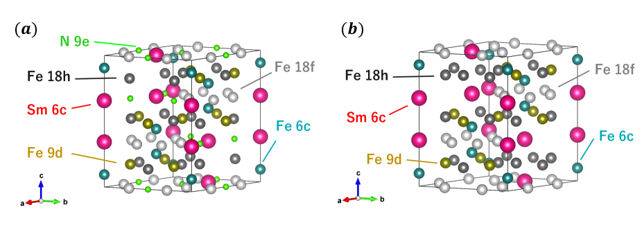
Figure 1: Crystal structures of the hexagonal unit cell and non-equivalent atomic positions of (a) Sm₂Fe₁₇N₃ Inami and (b) Sm₂Fe₁₇.Teresiak

III Results and Discussion

III.1 Electronic structure

We explain the calculated electronic structure for $\textrm{Sm}_{2}\textrm{Fe}_{17}$ and $\textrm{Sm}_{2}\textrm{Fe}_{17}\textrm{N}_{3}$. We show the spin magnetic moments of the Fe ions on each site, the total spin magnetic moments in the cell except the contribution from the Sm spin magnetic moments, and the total magnetic moments in the unit cell at 0K in Table 3, for comparison with the results of previous studiessteinbeck ; ogura . The total magnetic moments in the unit cell are calculated by Eq. (1) and Eq. (13), because the magnetic moments of the Sm ions contain the contribution from the orbital magnetic moments of 4f orbitals. The nearest neighbor sites for the Sm ions in $\textrm{Sm}_{2}\textrm{Fe}_{17}$ are 18f sites. In contrast, the nearest neighbor sites for the Sm ions in $\textrm{Sm}_{2}\textrm{Fe}_{17}\textrm{N}_{3}$ are 18h sitessteinbeck ; Inami . The difference of the valency does not affect the spin magnetic moments of each site drastically. We find that the nitrogenation causes the enhancement of the magnetic moments at 9d sites and reduction of those at 18f sites in both valency. Similar effects are discussed in Ogura $et\ al.$ However, no enhancement of magnetic moments at 6c sites was found in this work. We note that the magnetic moments of each Fe site in trivalent $\textrm{Sm}_{2}\textrm{Fe}_{17}$ are quite different from the results of Steinbeck $et\ al$., especially on 9d sites, and the magnetic moments of each Fe site in trivalent $\textrm{Sm}_{2}\textrm{Fe}_{17}\textrm{N}_{3}$ are similar to their results except that of 6c sitessteinbeck . For the trivalent configuration, we can see that the total magnetic moments of Sm ions in $\textrm{Sm}_{2}\textrm{Fe}_{17}$ and $\textrm{Sm}_{2}\textrm{Fe}_{17}\textrm{N}_{3}$ are $0.48\mu_{\textrm{B}}$ and $0.41\mu_{\textrm{B}}$, respectively. In contrast, for the divalent configuration, we can see the negative contribution; the total magnetic moments of Sm ions are $-2.70\mu_{\textrm{B}}$ and $-2.68\mu_{\textrm{B}}$ for $\textrm{Sm}_{2}\textrm{Fe}_{17}$ and $\textrm{Sm}_{2}\textrm{Fe}_{17}\textrm{N}_{3}$, respectively. The comparison of the calculated total magnetic moment at low temperature with experimentally measured values are discussed in sections III. B and III. C. Next, we show the CFPs $A_{l}^{m}\langle r^{l}\rangle$ calculated by Eq. (6) in Table 4. We can see that the CFPs $A_{l}^{m}\langle r^{l}\rangle$ of $\textrm{Sm}_{2}\textrm{Fe}_{17}\textrm{N}_{3}$ do not change drastically, except $A_{2}^{0}\langle r^{2}\rangle$, when we change the valency of the Sm ions. We also note that the values of $A_{2}^{0}\langle r^{2}\rangle$ for $\textrm{Sm}_{2}\textrm{Fe}_{17}\textrm{N}_{3}$ are the largest regardless of the its valency. This implies that $\textrm{Sm}_{2}\textrm{Fe}_{17}\textrm{N}_{3}$ shows uniaxial anisotropy, regardless of the valency of the Sm ions. However, we can see that the CFP $A_{2}^{0}\langle r^{2}\rangle$ of $\textrm{Sm}_{2}\textrm{Fe}_{17}$ is quite different in trivalent and divalent results. $A_{2}^{0}\langle r^{2}\rangle$ in the trivalent result is the largest among the CFPs; however, $A_{2}^{0}\langle r^{2}\rangle$ in the divalent result is quite small compared with the others. This implies that the difference of the valency of the Sm ions causes the change of the anisotropy of the system.

Table 3: Spin magnetic moments in unit $\mu_{\textrm{B}}$ of each Fe ion, total spin magnetic moment in the cell except the contribution from the Sm, and total magnetic moment per unit cell calculated by our effective single-ion model for each valency, with comparison to previous workssteinbeck ; ogura .

	Valency	6c	9d	18f	18h	$\bm{M}_{\textrm{Fe}}(0)$	Total
Present work
Sm2Fe17	Sm3+	2.67	2.21	2.49	2.39	39.72	40.19
	Sm2+	2.71	2.20	2.50	2.42	41.06	35.66
Present work
Sm2Fe17N3	Sm3+	2.65	2.48	2.18	2.36	38.80	39.41
	Sm2+	2.69	2.49	2.10	2.40	38.96	33.61
Steinbeck $et\ al.$steinbeck
Sm2Fe17	Sm3+	2.41	1.57	2.22	2.02	–	–
Sm2Fe17N3	Sm3+	2.36	2.45	2.13	2.42	–	–
Ogura $et\ al.$ogura
Sm2Fe17	–	2.53	2.15	2.42	2.17	–	–
Sm2Fe17N3	–	2.92	2.84	2.14	2.12	–	–

Table 4: The crystal field parameters $A_{l}^{m}\langle r^{l}\rangle$ [K] and the amplitude of the exchange mean-field $|\boldmath{H}_{\textrm{m}}$$(0)|$ [K] computed using first-principles calculations, and the spin-orbit coupling constants $\lambda$ [K] calculated from the experimental resultsMcClure .

	Valency	$A_{2}^{0}\langle r^{2}\rangle$	$A_{4}^{0}\langle r^{4}\rangle$	$A_{6}^{0}\langle r^{6}\rangle$	$A_{6}^{6}\langle r^{6}\rangle$	$|\boldmath{H}_{\textrm{m}}$$(0)|$	$\lambda$
Sm2Fe17	Sm3+	-176.1	-18.27	-0.122	43.07	354.1	350
	Sm2+	-8.07	-17.27	0.08	50.25	372.5	387
Sm2Fe17N3	Sm3+	-576.7	7.055	-1.213	29.85	176.3	350
	Sm2+	-718.5	11.27	-1.142	28.54	150.5	387

III.2 Magnetization curves of Sm₂Fe₁₇N₃

First, we look at the magnetization curves of Sm₂Fe₁₇N₃ calculated by the effective spin model. FIG. 2 (a) shows the magnetization curves along the [001] and [100] directions at $T=4.2$K, obtained by using the effective spin model with the trivalent Sm³⁺ (red) and the divalent Sm²⁺ (black). The experimental results for Sm₂Fe₁₇N_3.1 reported by Koyama $et\ al.$koyama are indicated by solid curves in FIG. 2 (a). We can clearly see that the [001] direction is the easy axis of this system, regardless of the valency of the Sm ions. However, as we noted in the section III. A, the saturation magnetizations $M_{\textrm{s}}$ at low temperature for Sm³⁺ and Sm²⁺ are clearly different. We also notice here that the results for the trivalent model in FIG. 2 (a) satisfactorily reproduce the experimentally observed magnetization curves. Thus, we can conclude that the Sm³⁺ electronic configuration is realized in Sm₂Fe₁₇N₃ compounds.

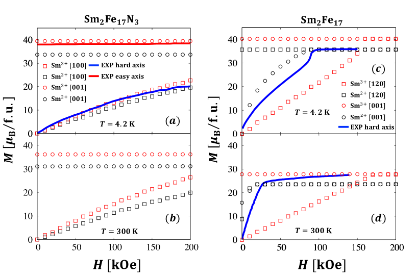
Figure 2: The calculated magnetization curves of Sm₂Fe₁₇N₃ at (a) 4.2K and (b) 300K and Sm₂Fe₁₇ at (c) 4.2K and (d) 300K. Sm²⁺ and Sm³⁺ are indicated by black and red plots, respectively, where $H$ [kOe] is the strength of the applied external magnetic field. In (a) and (b), the circles and squares indicate the results along the principal axis of [001] and [100] direction, respectively, and in (c) and (d), the circles and squares indicate the results along the principal axis of [001] and [120] direction, respectively. The experimental curves shown by red and blue lines in (a) at 4.2K are extracted from Koyama $et\ al$.koyama , in which the curves for 300K are not shown. The experimental curves in (c) and (d) at 4.2K and 300K are extracted from Diop $et\ al$. diop

The magnetization curves of Sm₂Fe₁₇N₃ at $T=300$K are shown in FIG. 2 (b), in the same manner as FIG. 2 (a). The saturation magnetization is reduced as changing the valency from Sm³⁺ to Sm²⁺; however, the qualitative behavior of the curves does not change from FIG. 2 (a).

III.3 Magnetization curves of Sm₂Fe₁₇

Next, we look at the magnetic properties of Sm₂Fe₁₇ described by the effective spin model. FIG. 2 (c) shows the calculated magnetization curves along the hard and easy directions at $T=4.2$K. We can clearly see that the magnetic anisotropy is qualitatively different between the systems with the trivalent Sm³⁺ and the divalent Sm²⁺ ions. When we assume the divalent Sm²⁺ configuration, the system shows planar anisotropy. Thus, the divalent results can reproduce the behavior that is experimentally observeddiop , as shown by a blue line in FIG. 2 (c) at 4.2K. We also show the curves at 300K in FIG. 2 (d). The qualitative behavior is almost the same as the results at 4.2K. It is noted that we can see the spin reorientation phenomenon. As stated in the Introduction, the orientation of the magnetization of this compound was experimentally found to deviate from the basal $a$-$b$ plane by as much as 10$\tcdegree$ at low temperatures diop . Moreover, at room temperature, the spontaneous magnetization lies within the basal plane itself. In our results, for the divalent configuration, when the external magnetic field is not applied, we cannot see the finite magnetization along the [001] direction at 4.2K; however, we can see the finite magnetization along the [001] direction at 300K. The divalent configuration results can qualitatively reproduce the magnetization curves for Sm₂Fe₁₇, but they cannot explain direction of the spontaneous magnetization at zero field. From our results, the curves assuming the divalent Sm²⁺ configuration can reproduce the experimental behaviors. However, as stated in the introduction, XAS experiments have shown that the Sm ions in Sm₂Fe₁₇N_x are trivalent Sm³⁺. One possible reason for this discrepancy is the CFPs. The open core method is used in our calculations. The Sm ions are assumed to be in an atomic-like state in this method. The hybridization of 4f and other orbitals is not taken into account in our CFPs. One possible method beyond the open core method is the Wannierization proposed by Novák et al.Pavel_Wannier In this method, 4f electrons are treated as valence electrons and projected using localized Wannier functions. Thus, we can incorporate the hybridization of 4f and other orbitals in this method. If the hybridization is taken into account, the CFPs and the anisotropy might be changed.

III.4 Anisotropy constants $K_{1}(T)$ and $K_{2}(T)$

We show the temperature dependence of the magnetic anisotropy constants $K_{1}(T)$ and $K_{2}(T)$ of Sm₂Fe₁₇N₃ and Sm₂Fe₁₇ in FIG. 3 (a) and (b), respectively. The anisotropy constants $K_{1}(T)$ and $K_{2}(T)$ of Sm₂Fe₁₇N₃ shown in FIG. 3 (a) are always positive regardless of the valency of the Sm ions. The total anisotropy constants $K_{1}(T)$ which include $K_{\textrm{Fe}}$, at 4.2K and 300K for each valency are indicated by triangles. The total anisotropy constants $K_{1}$($T$) are positive at 4.2K and 300K and close to the values measured by Wirth $et\ al.$Wirth at low temperature. This implies that Sm₂Fe₁₇N₃ shows uniaxial anisotropy at any temperature. The temperature dependence of $K_{1}(T)$ and $K_{2}(T)$ of Sm₂Fe₁₇ is shown in FIG. 3 (b) . We can see that the calculation results with trivalent Sm³⁺ show positive $K_{1}(T)$ and $K_{2}(T)$ at any temperature. Therefore, Sm₂Fe₁₇ with trivalent Sm³⁺ would show uniaxial anisotropy. In contrast, we can see negative $K_{1}(T)$ in the results with divalent Sm²⁺ configuration. The total anisotropy constants are also shown in the same manner as Sm₂Fe₁₇N₃ in FIG. 3 (a). Our total anisotropy constant for Sm²⁺ is close to the experimental values shown by Brennan $et\ al.\cite[cite]{\@@bibref{Authors Phrase1YearPhrase2}{Brennan}{\@@citephrase{(}}{\@@citephrase{)}}}$ and Isnard $et\ al.\cite[cite]{\@@bibref{Authors Phrase1YearPhrase2}{Isnard}{\@@citephrase{(}}{\@@citephrase{)}}}$ at low temperature. At 300K, our result is in good agreement with the value measured by Isnard $et\ al.$Isnard , where $K_{1}$ is $-1.75$ $[\textrm{MJ}/\textrm{m}^{3}]$ at 300K. Our total anisotropy constants $K_{1}$ for Sm²⁺ are negative at 4.2K and 300K. This implies that Sm₂Fe₁₇ with divalent Sm²⁺ would show planar anisotropy at low temperature. From the calculated anisotropy constants, the experimentally measured magnetization curve for Sm₂Fe₁₇N₃ can be explained by both results; however, the curve for Sm₂Fe₁₇ can be explained only by the divalent results.

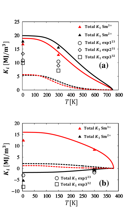
Figure 3: The calculated magnetic anisotropy constants $K_{1}$ (solid lines) and $K_{2}$ (dashed lines) per two Sm ions in (a) Sm₂Fe₁₇N₃ and (b) Sm₂Fe₁₇ with Sm³⁺ (red lines) or Sm²⁺ (black lines) electronic configuration. The total anisotropy constants $K_{1}$ with Fe sublattice contribution $K_{\textrm{Fe}}$ are indicated by red (Sm³⁺) and black (Sm²⁺) triangles. The open shapes indicate the experimentally measured values of $K_{1}$; the open circles correspond to the values of Brennan ${et\ al}$.Brennan , the open squares correspond to the values of Isnard ${et\ al}$.Isnard , and the open diamonds correspond to the values of Wirth ${et\ al}$.Wirth

IV Summary

In this work, we have calculated the magnetization curves and the temperature dependence of the anisotropy constants of Sm₂Fe₁₇ and Sm₂Fe₁₇N₃ by using the effective spin model based on first-principles calculations with the open core method. We showed that for Sm₂Fe₁₇N₃ the curves generated by the Sm³⁺ model are in good agreement with the experimentally measured curves. The total anisotropy constants $K_{1}$($T$) calculated for Sm₂Fe₁₇N₃ assuming Sm³⁺ and Sm²⁺ qualitatively reproduce the experimentally measured behavior, with the results from Sm³⁺ close to the experimental value. In contrast, the results for Sm₂Fe₁₇ assuming Sm²⁺ are consistent with the experimentally measured curves. In addition, the temperature dependence of the total anisotropy constants for Sm²⁺ is consistent with experimentally observed behavior. However, previously reported XAS experimentsXAS have found that the Sm ions in Sm₂Fe₁₇N_x are trivalent configuration regardless of the nitrogen content $x$.
It is noted that the effective spin model based on DFT calculations with the open core method might not be able to describe the magnetic properties of Sm₂Fe₁₇. One possible reason for this disagreement is that the hybridization effects between the 4f orbitals of the Sm ions and other orbitals cannot be included in the CFPs by using the open core method. In the open core method, 4f orbitals are treated as atomic-like core states and the valence effects of them are completely neglected. Taking the valence effects into account might change the CFPs and the magnetic anisotropy of the systems. For more precise investigation, further research should apply a more realistic method, such as the Wannierization method, Pavel_Wannier ; yoshi_Wannier that can incorporate the hybridization effects of 4f electrons and other orbitals to evaluate the CFPs.

- (1) L. V. B. Diop, M. D. Kuz’min, K. P. Skokov, D. Yu. Karpenkov, and O. Gutfleisch, Phys. Rev. B 94, 144413 (2016).
- (2) B. I. Min, J.-S. Kang, J. H. Hong, S. W. Jung, J. I. Jeong, Y. P. Lee, S. D. Choi, W. Y. Lee, C. J. Yang, and C. G. Olson, J. Phys.: Condens. Matter 5, 6911 (1993).
- (3) L. Steinbeck, M. Richter, U. Nitzsche, and H. Eschrig, Phys. Rev. B 53, 7111 (1996).
- (4) Yu. V. Knyazev, Yu. I. Kuz’min, A. G. Kuchin, A. V. Lukoyanov, and I. A. Nekrasov, J. Phys.: Condens. Matter 19, 116215 (2007).
- (5) T. Pandey, M.-H. Du, and D. S. Parker, Phys. Rev. Appl. 9, 034002 (2018).
- (6) K. Buschow, Rep. Prog. Phys. 54, 1123 (1991).
- (7) D. McNeely and H. Oesterrreicher, J. Less-Common Met. 44, 183 (1976).
- (8) M. Ogura, A. Mashiyama, and H. Akai, J. Phys. Soc. Jpn. 84, 084702 (2015).
- (9) X. C. Kou, F. R. de Boer, R. Grössinger, G. Wiesinger, H. Suzuki, H. Kitazawa, T. Takamasu, and G. Kido, J. Magn. Magn. Mater. 177–181, 1002 (1998).
- (10) T. W. Capehart, R. K. Mishra, and F. E. Pinkerton, Appl. Phys. Lett. 58, 1395 (1991).
- (11) H. W. de Wijin, A. M. van Diepen, and K. H. J. Buschow, Phys. Rev. B 7, 524 (1973).
- (12) S. G. Sankar, V. U. S. Rao, E. Segal, W. E. Wallace, W. G. D. Frederick, and H. J. Garrett, Phys. Rev. B 11, 435 (1975).
- (13) M. Yamada, H. Kato, H. Yamamoto, and Y. Nakagawa, Phys. Rev. B 38, 620 (1988).
- (14) M. Richter J. Phys. D: Appl. Phys. 31 1017 (1998).
- (15) J. Franse and R. Radwański, in Handbook of Magnetic Materials, edited by K. H. J. Buschow (North-Holland, Amsterdam, 1993), Vol. 7.
- (16) T. Yoshioka, and H. Tsuchiura, Appl. Phys. Lett. 112, 162405 (2018).
- (17) T. Yoshioka, H. Tsuchiura, and P. Novák, Phys. Rev. B 102, 184410 (2020).
- (18) P. Novák, Phys. Stat. Sol. B 198, 729 (1996).
- (19) M. Diviš, K. Schwarz, P. Blaha, G. Hilsher, H. Michor, and S. Khmelevskyi, Phys. Rev. B 62, 6774 (2000).
- (20) M. Diviš, J. Rusz, H. Michor, G. Hilsher, P. Blaha, and K. Schwarz, J. Alloys Compd. 403, 29 (2005).
- (21) P. Blaha, K. Schwarz, G. K. H. Madsen, D. Kvasnicka, and J. Luitz, WIEN2k, An Augmented Plane Wave + Local Orbitals Program for Calculating Crystal Properties (Karlheinz Schwarz, TU Wien, Austria, 2001).
- (22) N. Inami, Y. Takeuchi, T. Koide, T. Iriyama, M. Yamada and Y. Nakagawa, J. Appl. Phys. 115, 17A712 (2014).
- (23) S. Brennan, R. Skomski, O. Cugat and J. M. D. Coey, J. Magn. Magn. Mater. 140–144, 971 (1995).
- (24) M. D. Kuz’min, Phys. Rev. Lett. 94, 107204 (2005).
- (25) K. Koyama and H. Fujii, Phys. Rev. B 61, 9475 (2000).
- (26) R. Sasaki, D. Miura, and A. Sakuma Appl. Phys. Express 8, 043004 (2015).
- (27) M. S. S. Brooks, L. Nördstrom, and B. Johansson, J. Phys. Condens. Matter 3, (1991).
- (28) A. Teresiak, M. Kubis, N. Mattern, K.-H. Mller, and B. Wolf, J. Alloys Compd. 319, 168 (2001).
- (29) D. S. McClure, Solid State Phys. 9, 399–525 (1959).
- (30) P. Novák, K. Knížek, and J. Kuneš, Phys. Rev. B 87, 205139 (2013).
- (31) S. Wirth, M. Wolf, K.-H. Müller, R. Skomski, S. Brennan, and J. M. D. Coey, IEEE Trans. Magn. 32, 4746 (1996).
- (32) O. Isnard, S. Miraglia, M. Guillot, and D. Fruchart, J. Appl. Phys. 75, 5988 (1994).
- (33) T. Yoshioka, H. Tsuchiura, and P. Novák, Mater. Res. Innov. 19, S3 (2015).