Dicke States Generation via Selective Interactions in Dicke-Stark Model

Abstract

We propose a method to create selective interactions with Dicke-Stark model by means of time-dependent perturbation theory. By choosing the proper rotating framework, we find that the time oscillating terms depend on the number of atomic excitations and the number of photonic excitations. Consequently, the Rabi oscillation between selective states can be realized by properly choosing the frequency of the two-level system. The second order selective interactions can also be studied with this method. Then various states such as Dicke states, superposition of Dicke states and GHZ states can be created by means of such selective interactions. The numerical results show that high fidelity Dicke states and Greenberger-Horne-Zeilinger states can be created by choosing the proper frequency of two-level system and controlling the evolution time.

I Introduction

Quantum entanglement is one of the most prominent properties of quantum states that has no classical analog Horodecki et al. (2009). So far, a variety types entanglement states have been studied theoretically and experimentally Greenberger et al. (1989); Pan et al. (2012); Dür et al. (2000); Briegel et al. (2009). It has also motivated a variety of quantum protocols in quantum information theory Nielsen and Chuang (2010), such as teleportation Bennett et al. (1993), dense coding Bennett and Wiesner (1992), and quantum key distribution Ekert (1991). An important type of entangled states among them is the highly entangled Dicke states, which was firstly introduced in 1954 by Dicke Dicke (1954). Up to now, a growing number of efforts have been devoted to generate Dicke states Stockton et al. (2004); Masson and Parkins (2019); Wu et al. (2017); Prevedel et al. (2009); Shao et al. (2010), as well as superposition Dicke states, in a wide variety of quantum platforms, such as trapped ions Cirac et al. (1994); Unanyan and Fleischhauer (2003) and circuit QED system Kasture (2018); Hong and Lee (2002); Xiao et al. (2005); Yu et al. (2003); Ran et al. (2018).

On the other hand, selective interactions have a wide range of applications in quantum information theory, such as entanglement states generation. Such special interactions arise from the possibility of tuning to resonance transitions inside a chosen Hilbert subspace, while leaving other transitions dispersive Solano et al. (2001). In Solano et al. (2000), Solano et al proposed the selective interactions permits to manipulate motional states in two trapped ions. Recently, in  Cong et al. (2020), Cong et al studied the selective $k$-photonic interactions in the quantum Rabi model with Stark term, which is termed Rabi-Stark model Grimsmo and Parkins (2013a, 2014); Eckle and Johannesson (2017) and selective interactions can be used to create photonic Fock states. Such model attract much attentions in recent years Maciejewski et al. (2015); Xie et al. (2019); Xie and Chen (2019). The Stark term plays an important role in dynamical selectivity. This nonlinear coupling term was also added to the Dicke model Garraway (2011); Gopalakrishnan et al. (2011); Bastidas et al. (2012); Abdel-Rady et al. (2017), which is a fundamental model of quantum optics to describe the interactions between light and matter Kirton et al. (2019); Bhaseen et al. (2012); Dimer et al. (2007); Grimsmo and Parkins (2013b); Zhang et al. (2018). The existence of Stark term in the Dicke-Stark (DS) model can be used to create nonlinear energy levels, which will be used to generate entangled states selectively.

In this work, we will study the selective interactions in the DS model. Choosing proper rotating frame, we find the time-varying terms depend on the number of excitations. Then one can choose proper frequencies of the system to obtain selective Tavis-Cummings (TC) Tavis and Cummings (1968) or anti-TC interactions from the DS model Günter et al. (2009); Niemczyk et al. (2010); Rossatto et al. (2017); Frisk Kockum et al. (2019); Forn-Díaz et al. (2019). Considering the second order effects, the two-atom selective interactions also can be obtained. Acting such effective interactions on the pre-selective initial states, one can obtain the selective target Dicke states, as well as superposition of Dicke states. Finally, the validity of our proposal is studied with numerical simulations. The results show that one can obtain high fidelity by properly choosing frequencies of two-level systems.

II The derivation of the effective Hamiltonian

The Hamiltonian of DS model, describing the Dicke model with Stark term, is given by ($\hbar=1$)

$$\hat{H}_{\rm DS}=\hat{H}_{0}+\hat{H}_{\rm int},$$ (1)

where

$$\begin{split}\hat{H}_{0}&=\frac{\omega_{q}}{2}\sum_{j=1}^{N}\hat{\sigma}_{j}^{z}+\omega_{r}\hat{a}^{\dagger}\hat{a}+\frac{U}{2N}\hat{a}^{\dagger}\hat{a}\sum_{j=1}^{N}\hat{\sigma}_{j}^{z},\\ \hat{H}_{\rm int}&=\frac{\lambda}{\sqrt{N}}\sum_{j=1}^{N}(\hat{a}+\hat{a}^{\dagger})\hat{\sigma}_{j}^{x}.\end{split}$$

This Hamiltonian describes $N$ two-level systems (or qubits) with uniform transition frequency $\omega_{q}$ coupling to a single mode bosonic field with frequency $\omega_{r}$. Here we assume the coupling strength between each qubit and resonator is uniform. The parameter $U$ is the coupling strength of the Stark term. $\hat{a}$ and $\hat{a}^{\dagger}$ denote the annihilation and creation operators of the resonator respectively. The $j$-th qubit operators are $\hat{\sigma}_{j}^{x}=|e_{j}\rangle\langle g_{j}|+|g_{j}\rangle\langle e_{j}|$, $\hat{\sigma}_{j}^{y}=-i(|e_{j}\rangle\langle g_{j}|-|g_{j}\rangle\langle e_{j}|)$ and $\hat{\sigma}_{j}^{z}=|e_{j}\rangle\langle e_{j}|-|g_{j}\rangle\langle g_{j}|$ with $|g_{j}\rangle$ and $|e_{j}\rangle$ be the ground and excited states for the $j$-th qubit. By utilizing the relation $\hat{\sigma}_{j}^{\pm}=(\hat{\sigma}_{j}^{x}\pm i\hat{\sigma}_{j}^{y})/2$, the Dicke coupling term in the Hamiltonian Eq. (1) can be rewritten as following two terms $(\lambda/\sqrt{N})\sum_{j=1}^{N}(\hat{a}\hat{\sigma}_{j}^{+}+\hat{a}^{\dagger}\hat{\sigma}_{j}^{-})$ and $(\lambda/\sqrt{N})\sum_{j=1}^{N}(\hat{a}^{\dagger}\hat{\sigma}_{j}^{+}+\hat{a}\hat{\sigma}_{j}^{-})$, which corresponding to rotating and counter-rotating terms. In the situation where the qubits are near resonance with the resonator and the coupling between qubits and resonator are much smaller than the transition frequency of qubits and frequency of the resonator, the rotating-wave-approximation (RWA) is valid. In this case, we can drop the counter-rotating term safely. Consequently, the Hamiltonian in Eq. (1) reduced to the Tavis-Cummings (TC) model with Stark term. The Dicke model with Stark term in Eq. (1) depends on the following atomic collective operators $\hat{J}_{\alpha}=\sum_{j=1}^{N}\hat{\sigma}_{j}^{\alpha}$ with $\alpha=x,z$. In terms of atomic collective operators, the Hamiltonian in Eq. (1) reads

$$\begin{split}\hat{H}_{\rm DS}&=\frac{\omega_{q}}{2}\hat{J}_{z}+\omega_{r}\hat{a}^{\dagger}\hat{a}+\frac{\lambda}{\sqrt{N}}(\hat{a}+\hat{a}^{\dagger})\hat{J}_{x}+\frac{U}{2N}\hat{a}^{\dagger}\hat{a}\hat{J}_{z}.\\ \end{split}$$ (2)

To obtain a closed analytical description, we introduce the normalized Dicke states with $k$ atomic excitations Noguchi et al. (2012); Zhou et al. (2011); Hume et al. (2009)

$$\left|D_{N}^{k}\right\rangle\equiv\left(C^{N}_{k}\right)^{-1/2}\sum_{m=1}^{C^{N}_{k}}P_{m}|\overbrace{e_{j_{1}},e_{j_{2}}\cdots,e_{j_{k}}}^{k},\overbrace{g_{j_{k+1}},\cdots,g_{j_{N}}}^{N-k}\rangle.$$ (3)

Here $\sum_{m=1}^{C^{N}_{k}}P_{m}(\cdots)$ indicates the sum over all particle permutations and $C^{N}_{k}=N!/[k!(N-k)!]$. In the Dicke states basis, the collective operators can be reduced to $\hat{J}_{x,z}^{D}$ as

$$\begin{split}\hat{J}_{x}^{D}&=\sum_{k=0}^{N}f(k)(|D_{N}^{k+1}\rangle\langle D_{N}^{k}|+|D_{N}^{k}\rangle\langle D_{N}^{k+1}|),\\ \hat{J}_{z}^{D}&=\sum_{k=0}^{N}(2k-N)|D_{N}^{k}\rangle\langle D_{N}^{k}|,\end{split}$$ (4)

where $f(k)=\sqrt{(k+1)(N-k)}$. In terms of Dicke states and Fock states, the Hamiltonian Eq. (1) can be recast as follows

$$\begin{split}&\hat{H}^{D}_{0}=\sum_{n,k}\left[\left(\omega_{q}+n\frac{U}{N}\right)\left(k-\frac{N}{2}\right)+n\omega_{r}\right]\hat{D}_{k,k}\otimes\hat{A}_{n,n},\\ &\hat{H}^{D}_{\rm int}=\sum_{n,k}\Omega_{nk}(\lambda)(\hat{D}_{k+1,k}+\hat{D}_{k,k+1})\otimes(\hat{A}_{n,n+1}+\hat{A}_{n+1,n}),\end{split}$$ (5)

where $\Omega_{nk}(\lambda)=\lambda f(k)\sqrt{n+1}/\sqrt{N}$, $\hat{D}_{k,k^{\prime}}=|D_{N}^{k}\rangle\langle D_{N}^{k^{\prime}}|$, and $\hat{A}_{n,n^{\prime}}=|n\rangle\langle n^{\prime}|$. Moving to the interaction picture with respect to $\hat{H}_{0}^{D}$, one obtains the following transformed Hamiltonian

$$\begin{split}\hat{H}_{I}^{D}(t)&=\hat{R}^{\dagger}(t)\left(\hat{H}_{0}^{D}+\hat{H}_{\rm int}^{D}\right)\hat{R}(t)+i\left[\partial_{t}\hat{R}^{\dagger}(t)\right]\hat{R}(t)\\ &=\hat{H}_{\rm TC}^{D}(t)+\hat{H}_{\rm aTC}^{D}(t),\end{split}$$ (6)

where $\hat{R}(t)=\exp(-i\hat{H}_{0}^{D}t)$. The TC and anti-TC Hamiltonian in the rotating framework are as follows

$$\begin{split}&\hat{H}_{\rm TC}^{D}(t)=\sum_{n,k}\Omega_{nk}(\lambda)\left(\hat{D}_{k+1,k}\otimes\hat{A}_{n,n+1}e^{i\delta_{nk}^{-}t}+{\rm H.c.}\right),\\ &\hat{H}_{\rm aTC}^{D}(t)=\sum_{n,k}\Omega_{nk}(\lambda)\left(\hat{D}_{k+1,k}\otimes\hat{A}_{n+1,n}e^{i\delta_{nk}^{+}t}+{\rm H.c.}\right).\end{split}$$ (7)

Here $\delta_{nk}^{+}=\omega_{r}+\omega_{q}+U(n+k+1-N/2)/N$, $\delta_{nk}^{-}=\omega_{q}-\omega_{r}+U(n-k+N/2)/N$, and H.c. denotes the Hermitian conjugate. Obviously, the resonance frequencies $\delta_{nk}^{\pm}$ depend on the photon number $n$ and the atomic excitation number $k$. We can tune the parameters to obtain the resonant transition, and the other transitions are off-resonance. If we fix the photon number $n=n_{0}$ in the initial states, the oscillation frequencies $\delta_{nk}^{\pm}$ only depend on $k$. Consequently, the designed interactions depend on $k$ can be realized. If $U=0$, the detunings $\delta_{nk}^{\pm}$ are $n$ and $k$ independent. For $|\delta^{+}|\gg|\Omega_{nk}(\lambda)|$ and $\delta^{-}=0$, $\hat{H}^{D}_{\rm TC}$ is recovered when fast oscillating terms are averaged out by utilizing the RWA. Under these conditions, the dynamics lead to Rabi oscillations between the states $|D^{k+1}_{N}\rangle\otimes|n\rangle\leftrightarrow|D^{k}_{N}\rangle\otimes|n+1\rangle$ for each pair of $n$ and $k$ with the Rabi frequency $\Omega_{nk}(\lambda)$. On the contrary, the conditions $|\delta^{-}|\gg|\Omega_{nk}(\lambda)|$ and $\delta^{+}=0$ lead to an anti-TC resonant interaction. Consequently, the dynamics lead to Rabi oscillations between states $|D^{k}_{N}\rangle\otimes|n\rangle$ and $|D^{k+1}_{N}\rangle\otimes|n+1\rangle$. The interactions realized in such case are not selective as they apply to all pairs of $n$ and $k$.

The presence of a non-zero Stark coupling $U$ makes the TC and anti-TC resonant interactions different for the Fock state labeled by $n$ and Dicke state labeled by $k$. Given different values of $n$ and $k$, it is possible to adjust the value of the parameters to identify a resonance condition that applies only for a selected state. We note that if $\delta_{n_{0}+m,k_{0}+m}^{-}=0$, $|\delta_{n\neq n_{0}+m,k\neq k_{0}+m}^{-}|\gg|\Omega_{n\neq n_{0}+m,k\neq k_{0}+m}(\lambda)|$ and $|\delta_{nk}^{+}|\gg|\Omega_{nk}(\lambda)|$, the dynamics of Hamiltonian Eq. (6) will produce a selective TC interaction, which leads to transitions between $|D^{k_{0}+m+1}_{N}\rangle\otimes|n_{0}+m\rangle$ and $|D^{k_{0}+m}_{N}\rangle\otimes|n_{0}+m+1\rangle$. If the initial state is prepared to the fix photon number $n=n_{0}$ (i.e., $m=0$), only interaction between $|D^{k_{0}+1}_{N}\rangle\otimes|n_{0}\rangle$ and $|D^{k_{0}}_{N}\rangle\otimes|n_{0}+1\rangle$ is survived. The effective Hamiltonian for such selective TC interaction reads

$$\hat{H}_{\rm TC}^{\rm eff}=\Omega_{n_{0},k_{0}}(\lambda)\left(\hat{D}_{k_{0}+1,k_{0}}\otimes\hat{A}_{n_{0},n_{0}+1}+{\rm H.c.}\right).$$ (8)

The case in which $\delta_{n_{0}+m,k_{0}-m}^{+}=0$, $|\delta_{n\neq n_{0}+m,k\neq k_{0}-m}^{+}|\gg|\Omega_{n\neq n_{0}+m,k\neq k_{0}-m}(\lambda)|$ and $\delta_{nk}^{-}\gg\Omega_{nk}(\lambda)$ leads to transitions between $|D^{k_{0}-m}_{N}\rangle\otimes|n_{0}+m\rangle$ and $|D^{k_{0}-m+1}_{N}\rangle\otimes|n_{0}+m+1\rangle$. If the initial state is prepared to the fix photon number $n=n_{0}$ (i.e., $m=0$), only interaction between $|D^{k_{0}}_{N}\rangle\otimes|n_{0}\rangle$ and $|D^{k_{0}+1}_{N}\rangle\otimes|n_{0}+1\rangle$ is survived. The effective Hamiltonian for the anti-TC interaction reads

$$\hat{H}_{\rm aTC}^{\rm eff}=\Omega_{n_{0},k_{0}}(\lambda)\left(\hat{D}_{k_{0}+1,k_{0}}\otimes\hat{A}_{n_{0}+1,n_{0}}+{\rm H.c.}\right).$$ (9)

The sketches of energy level for the selected TC and anti-TC model are shown in Fig. 1. The Fig. 1(a) shows that only selected states $|D_{N}^{k_{0}}\rangle\otimes|n_{0}+1\rangle$ and $|D_{N}^{k_{0}+1}\rangle\otimes|n_{0}\rangle$ are resonant and they are detuning with the other states. The effective Hamiltonian describing such selected TC interaction are given in Eq. (8). The Fig. 1(b) shows that selected states $|D_{N}^{k_{0}}\rangle\otimes|n_{0}\rangle$ and $|D_{N}^{k_{0}+1}\rangle\otimes|n_{0}+1\rangle$ are resonant and they are detuning with the other states.

The selective resonance peaks for initial states with different number of atomic excitations are shown in Fig. 2, where four two-level systems are considered. The Fig. 2(a) shows the Hamiltonian acts on the initial states $|D_{4}^{k_{0}}\rangle\otimes|1\rangle$ during a time $t=\pi/(2\Omega_{n_{0},k_{0}}(\lambda))$. The results show that only the resonance transition between $|D_{4}^{k_{0}}\rangle\otimes|1\rangle$ and $|D_{4}^{k_{0}+1}\rangle\otimes|0\rangle$ can occur. The Fig. 2(b) shows the Hamiltonian acts on the initial state $|D_{4}^{k_{0}}\rangle\otimes|0\rangle$, and only the resonance transition between $|D_{4}^{k_{0}}\rangle\otimes|0\rangle$ and $|D_{4}^{k_{0}+1}\rangle\otimes|1\rangle$ can occur. The average atomic excitation number $\langle\hat{N}_{q}\rangle$ also shows the oscillatory behavior near the resonance peaks. These behaviors can be explained by Rabi oscillating with small detuning. We take the transition $|D_{4}^{0}\rangle\otimes|1\rangle\leftrightarrow|D_{4}^{1}\rangle\otimes|0\rangle$ as an example (the solid black line in left panel of fig. 2). There is a resonance peak locate at $(\omega_{r}-\omega_{q})/\omega_{r}=-0.250$. If we consider there is a small detuning $\delta$, the effective Hamiltonian in Eq. (8) can be recast as follows

$$\hat{H}_{\rm TC}^{\rm eff}=\Omega_{1,0}(\lambda)\left(\hat{D}_{1,0}\otimes\hat{A}_{0,1}e^{i\delta t}+{\rm H.c.}\right).$$ (10)

Then the probability of the system in state $|D_{4}^{1}\rangle\otimes|0\rangle$ at time $t$ can be obtained as follows

$$P_{|D_{4}^{1}\rangle\otimes|0\rangle}(t)=\frac{4(\Omega_{1,0}(\lambda))^{2}}{4(\Omega_{1,0}(\lambda))^{2}+\delta^{2}}\sin^{2}\left(\frac{1}{2}\sqrt{4(\Omega_{1,0}(\lambda))^{2}+\delta^{2}}t\right).$$ (11)

At $t_{0}=\pi/(2\Omega_{1,0}(\lambda))$, we obtain the probabilities of the system in the state $|D_{4}^{1}\rangle\otimes|0\rangle$ is

$$P_{|D_{4}^{1}\rangle\otimes|0\rangle}(t_{0})=\frac{4(\Omega_{1,0}(\lambda))^{2}}{4(\Omega_{1,0}(\lambda))^{2}+\delta^{2}}\sin^{2}\left(\frac{t_{0}}{2}\sqrt{4(\Omega_{1,0}(\lambda))^{2}+\delta^{2}}\right).$$ (12)

Near the resonance peak, the probability and $\langle\hat{N}_{q}\rangle$ show oscillatory behavior. When the detuning $\delta=0$, the probabilities of the system in the state $|D_{4}^{1}\rangle\otimes|0\rangle$ will reach its maximum value $1$. With the increases of detuning, the amplitude of the oscillations is attenuated. Such similar behavior also is studied in Huang et al. (2017).

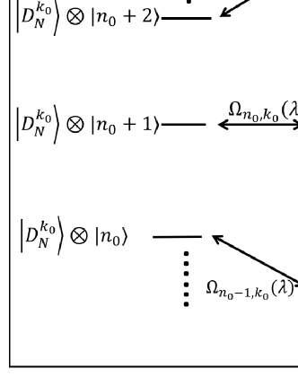
Figure 1: The sketches of energy level for the selected TC and anti-TC model: (a) shows that only selected states $|D_{N}^{k_{0}}\rangle\otimes|n_{0}+1\rangle$ and $|D_{N}^{k_{0}+1}\rangle\otimes|n_{0}\rangle$ are resonant and they are detuning with the other states; (b) shows that only selected states $|D_{N}^{k_{0}}\rangle\otimes|n_{0}\rangle$ and $|D_{N}^{k_{0}+1}\rangle\otimes|n_{0}+1\rangle$ are resonant and they are detuning with the other states.

The DS model not only can be used to produce single-atom excitation interactions, but also can be used to generate more than single-atom excitation interactions. To show multi-atom excitation process, we should consider higher order effective Hamiltonian. Here, we will consider two-atom excitation process. By means of the effective Hamiltonian method given in Shao et al. (2017), we will derive the second order effective Hamiltonian. If all terms in the Eq. (7) are fast-time varying terms, higher order effective Hamiltonian will dominate the dynamics. According to James and Jerke (2007), the second order Hamiltonian can be derived as follows

$$\begin{split}\hat{H}^{(2)}(t)&=\hat{H}_{0}^{(2)}+\hat{H}_{\rm TC}^{(2)}(t)+\hat{H}_{\rm aTC}^{(2)}(t)+\hat{H}_{r}^{(2)}(t)+\hat{H}_{a}^{(2)}(t),\end{split}$$ (13)

where

$$\begin{split}&\hat{H}_{0}^{(2)}=\sum_{n,k}\Delta_{n,k}\hat{D}_{k,k}\otimes\hat{A}_{n,n},\\ &\hat{H}_{\rm TC}^{(2)}(t)=\sum_{n,k}\Omega_{\rm TC}^{(2)}\left(\hat{D}_{k+2,k}\otimes\hat{A}_{n,n+2}e^{i\delta_{TC}^{(2)}(n,k)t}+{\rm H.c.}\right),\\ &\hat{H}_{\rm aTC}^{(2)}(t)=\sum_{n,k}\Omega_{\rm aTC}^{(2)}\left(\hat{D}_{k+2,k}\otimes\hat{A}_{n+2,n}e^{i\delta_{aTC}^{(2)}(n,k)t}+{\rm H.c.}\right),\\ &\hat{H}_{r}^{(2)}(t)=\sum_{n,k}\Omega_{r}^{(2)}\left(\hat{D}_{k+2,k}\otimes\hat{A}_{n,n}e^{i\delta_{r}^{(2)}(n)t}+{\rm H.c.}\right),\\ &\hat{H}_{a}^{(2)}(t)=\sum_{n,k}\Omega_{a}^{(2)}\left(\hat{D}_{k,k}\otimes\hat{A}_{n+2,n}e^{i\delta_{a}^{(2)}(k)t}+{\rm H.c.}\right).\end{split}$$ (14)

Here

$$\begin{split}&\Delta_{n,k}=\frac{\Omega^{2}_{n,k-1}(\lambda)}{\delta^{-}_{n,k-1}}+\frac{\Omega^{2}_{n-1,k-1}(\lambda)}{\delta^{+}_{n-1,k-1}}-\frac{\Omega^{2}_{n-1,k}(\lambda)}{\delta^{-}_{n-1,k}}-\frac{\Omega^{2}_{n,k}(\lambda)}{\delta^{+}_{n,k}},\\ &\Omega_{\rm TC}^{(2)}=\frac{1}{2}\Omega_{n,k+1}(\lambda)\Omega_{n+1,k}(\lambda)\left(\frac{1}{\delta_{n,k+1}^{-}}-\frac{1}{\delta_{n+1,k}^{-}}\right),\\ &\Omega_{\rm aTC}^{(2)}=\frac{1}{2}\Omega_{n,k}(\lambda)\Omega_{n+1,k+1}(\lambda)\left(\frac{1}{\delta_{n+1,k+1}^{+}}-\frac{1}{\delta_{n,k}^{+}}\right),\\ &\Omega_{r}^{(2)}=\frac{1}{2}\left(\Omega_{n-1,k}(\lambda)\Omega_{n-1,k+1}(\lambda)\left(\frac{1}{\delta_{n-1,k+1}^{+}}-\frac{1}{\delta_{n-1,k}^{-}}\right)+\Omega_{n,k}(\lambda)\Omega_{n,k+1}(\lambda)\left(\frac{1}{\delta_{n,k+1}^{-}}-\frac{1}{\delta_{n,k}^{+}}\right)\right),\\ &\Omega_{a}^{(2)}=\frac{1}{2}\left(\Omega_{n,k-1}(\lambda)\Omega_{n+1,k-1}(\lambda)\left(\frac{1}{\delta_{n+1,k-1}^{+}}+\frac{1}{\delta_{n,k-1}^{-}}\right)-\Omega_{n,k}(\lambda)\Omega_{n+1,k}(\lambda)\left(\frac{1}{\delta_{n,k}^{+}}+\frac{1}{\delta_{n+1,k}^{-}}\right)\right),\end{split}$$ (15)

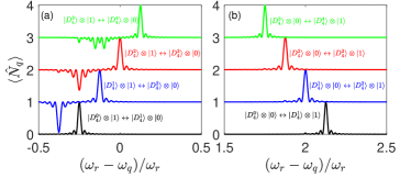
Figure 2: The selection interaction in Dicke-Stark model: (a) shows the resonance transition between $|D_{4}^{k_{0}}\rangle\otimes|1\rangle$ and $|D_{4}^{k_{0}+1}\rangle\otimes|0\rangle$, which controlled by the selected TC model in Eq. (8); (b) shows the resonance transition between $|D_{4}^{k_{0}}\rangle\otimes|0\rangle$ and $|D_{4}^{k_{0}+1}\rangle\otimes|1\rangle$, which controlled by the selected anti-TC model in Eq. (9). Other parameters are given as follows: $\omega_{r}=1$, $\lambda/\omega_{r}=0.006$ and $U/\omega_{r}=-0.5$. Here $\hat{N}_{q}=\sum_{j}^{N}\hat{\sigma}_{j}^{+}\hat{\sigma}_{j}^{-}$ denotes the atomic excitation operator.

and $\delta_{\rm TC}^{(2)}(n,k)=\delta_{n+1,k}^{-}+\delta_{n,k+1}^{-}$, $\delta_{\rm aTC}^{(2)}(n,k)=\delta_{n,k}^{+}+\delta_{n+1,k+1}^{+}$, $\delta_{r}^{(2)}(n,k)=\delta_{n,k}^{+}+\delta_{n,k+1}^{-}$, $\delta_{a}^{(2)}(n,k)=\delta_{n,k}^{+}-\delta_{n+1,k}^{-}$. The total excitation number conserved term $\hat{H}_{0}^{(2)}$ in Hamiltonian Eq. (13) is effective Stark shift. Moving to the rotating frame with respect to $\hat{R}_{s}(t)=e^{-i\hat{H}_{0}^{(2)}t}$, we obtain the following transformed Hamiltonian

$$\tilde{H}^{(2)}(t)=\tilde{H}^{(2)}_{\rm TC}(t)+\tilde{H}^{(2)}_{\rm aTC}(t)+\tilde{H}^{(2)}_{r}(t)+\tilde{H}^{(2)}_{a}(t),$$ (16)

where $\hat{\tilde{H}}^{(2)}_{\alpha}(t)=\hat{R}_{s}^{\dagger}(t)\hat{H}_{\alpha}^{(2)}\hat{R}_{s}(t)+i\left[\partial_{t}\hat{R}_{s}^{\dagger}(t)\right]\hat{R}_{s}(t)$ with $\alpha={\rm TC},~{}{\rm aTC},~{}r,~{}a$. Then the time oscillating frequency can be modified to $\tilde{\delta}_{\rm TC}^{(2)}(n,k)=\delta_{\rm TC}^{(2)}(n,k)+\Delta_{n,k+2}-\Delta_{n+2,k}$, $\tilde{\delta}_{\rm aTC}^{(2)}(n,k)=\delta_{\rm aTC}^{(2)}(n,k)+\Delta_{n+2,k+2}-\Delta_{n,k}$, $\tilde{\delta}_{r}^{(2)}(n,k)=\delta_{r}^{(2)}(n,k)+\Delta_{n,k+2}-\Delta_{n,k}$ and $\tilde{\delta}_{a}^{(2)}(n,k)=\delta_{a}^{(2)}(n,k)+\Delta_{n+2,k}-\Delta_{n,k}$. In the following, we will focus on the two-atom TC and anti-TC dynamics. Obviously, the time oscillating frequencies $\tilde{\delta}_{\rm TC}^{(2)}(n,k)$, $\tilde{\delta}_{\rm aTC}^{(2)}(n,k)$ depend on $n$ and $k$. In order to get an effective TC and anti-TC Hamiltonian, we can choose proper frequencies of two-level systems to make $\tilde{\delta}_{\rm TC}^{(2)}(n,k)=0$ or $\tilde{\delta}_{\rm aTC}^{(2)}(n,k)=0$ and the other time oscillating frequencies large greater than its corresponding effective coupling strength. Then the fast oscillating terms are averaged out by utilizing the RWA. By means of these conditions, we can achieve the so-called selective two photon TC and anti-TC model.

Under conditions $\tilde{\delta}_{\rm TC}^{(2)}(n_{0}+m,k_{0}+m)=0$, $|\tilde{\delta}_{\rm TC}^{(2)}(n\neq n_{0}+m,k\neq k_{0}+m)|\gg\Omega_{\rm TC}^{(2)}(n\neq n_{0}+m,k\neq k_{0}+m,\lambda)$ and $|\tilde{\delta}_{\alpha}^{(2)}(n,k)|\gg\Omega_{\alpha}^{(2)}(n,k,\lambda)$ with $\alpha={\rm aTC}$, $r$, or $a$, the dynamic evolution leads to transitions between $|D^{k_{0}+m+2}_{N}\rangle\otimes|n_{0}+m\rangle$ and $|D^{k_{0}+m}_{N}\rangle\otimes|n_{0}+m+2\rangle$. Fixing the photon number $n=n_{0}$ (i.e. $m=0$), the interaction between $|D^{k_{0}+2}_{N}\rangle\otimes|n_{0}\rangle$ and $|D^{k_{0}}_{N}\rangle\otimes|n_{0}+2\rangle$ is survived. The effective Hamiltonian for the TC interaction reads

$$\hat{H}_{\rm TC}^{(2)}=\Omega_{\rm TC}^{(2)}(n_{0},k_{0},\lambda)\left(\hat{D}_{k_{0}+2,k_{0}}\otimes\hat{A}_{n_{0},n_{0}+2}+{\rm H.c.}\right).$$ (17)

We also note that if $\tilde{\delta}_{\rm aTC}^{(2)}(n_{0}+m,k_{0}-m)=0$, $|\tilde{\delta}_{\rm aTC}^{(2)}(n\neq n_{0}+m,k\neq k_{0}-m)|\gg\Omega_{\rm aTC}^{(2)}(n\neq n_{0}+m,k\neq k_{0}-m,\lambda)$, $|\tilde{\delta}_{\alpha}^{(2)}(n,k)|\gg\Omega_{\alpha}^{(2)}(n,k,\lambda)$ with $\alpha={\rm TC}$, $r$, or $a$, only interaction between $|D^{k_{0}}_{N}\rangle\otimes|n_{0}\rangle$ and $|D^{k_{0}+2}_{N}\rangle\otimes|n_{0}+2\rangle$ is survived (i.e. $m=0$). The effective Hamiltonian for anti-TC interaction reads

$$\hat{H}_{\rm aTC}^{(2)}=\Omega_{\rm aTC}^{(2)}(n_{0},k_{0},\lambda)\left(\hat{D}_{k_{0}+2,k_{0}}\otimes\hat{A}_{n_{0}+2,n_{0}}+{\rm H.c.}\right).$$ (18)

The higher order dynamics can also be considered with this method. Then the higher order selective TC and anti-TC effective Hamiltonian can be achieved.

III The applications of selective interaction

In this section, we will show how to generate Dicke states and superposition of Dicke states with the selective TC and anti-TC interactions given in Sec. II. Here we will introduce our method by taking $N=4$.

III.1 Generation Dicke states with single-atom excitation TC and anti-TC model

Let initial state be $|\psi(0)\rangle=|D_{4}^{0}\rangle\otimes|0\rangle\equiv|g_{1}g_{2}g_{3}g_{4}\rangle\otimes|0\rangle$. We will show how to generate Dicke states with first order Hamiltonian given in Eqs. (8) and  (9) in several steps. First, one can tune the frequency of the two-level systems into the condition $\delta_{n_{0}=0,k_{0}=0}^{+}=0$. Applying the selective interaction in Eq. (9) to the initial state $|D_{4}^{0}\rangle\otimes|0\rangle$, one can obtain the superposition state $|\psi(t)\rangle=\cos\left(\Omega_{0,0}(\lambda)t\right)|D_{4}^{0}\rangle\otimes|0\rangle-i\sin\left(\Omega_{0,0}(\lambda)t\right)|D_{4}^{1}\rangle\otimes|1\rangle$. After a time period $T_{1}=t_{1}=\pi/(2\Omega_{0,0}(\lambda))$, we obtain the state $|\psi(t_{1})\rangle=|D_{4}^{1}\rangle\otimes|1\rangle$. When the qubit frequency is $\omega_{q}=-\omega_{r}+U/4$, we can see that the resonance peak appears in Fig. 3(a), and the average excitation number $\langle\hat{a}^{{\dagger}}\hat{a}\rangle$ and $\langle\hat{N}_{q}\rangle$ reach the maximum $1$. The Fig. 3(b) shows a perfect Rabi oscillation can only be realized in the pre-selected subspace $\left\{|D_{4}^{0}\rangle\otimes|0\rangle,{|D_{4}^{1}\rangle}\otimes|1\rangle\right\}$, while the population of the other quantum Dicke states is nearly zero. In Fig. 4, we switch on the selective interaction by tuning the frequency of the two-level systems to satisfy the condition $\delta_{n_{0}=0,k_{0}=1}^{-}=0$. Applying selective interaction on the state $|\psi(t_{1})\rangle=|D_{4}^{1}\rangle\otimes|1\rangle$ for a time period $T_{2}=t_{2}-t_{1}=\pi/(2\Omega_{0,1}(\lambda))$, we obtain the state $|\psi(t_{2})\rangle=|D_{4}^{2}\rangle\otimes|0\rangle$. Then tuning $\omega_{q}$ to satisfy the condition $\delta_{n_{0}=0,k_{0}=2}^{+}=0$ and acting the selective anti-TC interaction for a time period $T_{3}=t_{3}-t_{2}=\pi/(2\Omega_{0,2}(\lambda))$, we can be obtain the state $|\psi(t_{3})\rangle=|D_{4}^{3}\rangle\otimes|1\rangle$. The dynamics for the selective interaction are shown in Fig. 5. Finally, to obtain the Dicke state $|D_{4}^{4}\rangle$, we should tune the frequency $\omega_{q}$ to satisfy the condition $\delta_{n_{0}=0,k_{0}=3}^{-}=0$, and act the selective TC interaction on the state $|\psi(t_{3})\rangle$ for a time period $T_{4}=t_{4}-t_{3}=\pi/(2\Omega_{0,3}(\lambda))$. The final state is $|\psi(t_{4})\rangle=|D_{4}^{4}\rangle\otimes|0\rangle$. Tracing out the photon state, we obtained the Dicke state $|D_{4}^{4}\rangle$. As can be seen from Fig. 6, when the parameters and resonance frequency are properly selected, the desired target state can be successfully prepared. In all of these pictures, we present the average excitation number and the population of Dicke states with the parameters $\omega_{r}=1$, $\lambda=0.006\omega_{r}$ and $U=-0.5\omega_{r}$.

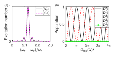
Figure 3: One-atom-excitation selective interactions of the Dicke-stark model. (a) After a time $T_{1}=\pi/(2\Omega_{0,0}(\lambda))$, we calculation the average number of excitations for different ratios of $(\omega_{r}-\omega_{q})/\omega_{r}$ with initial state $|D_{4}^{0}\rangle\otimes|0\rangle$, where the anti-TC peaks appears for $(\omega_{r}-\omega_{q})/\omega_{r}=2.125$ which corresponds to $\delta_{n_{0}=0,k_{0}=0}^{+}=0$; (b) The population of Dicke states as function of evolution time with initial state $|D_{4}^{0}\rangle$, and the resonance frequency locate at $(\omega_{r}-\omega_{q})/\omega_{r}=2.125$. The other parameters are given as follows: $\omega_{r}=1$, $\lambda/\omega_{r}=0.006$ and $U/\omega_{r}=-0.5$.

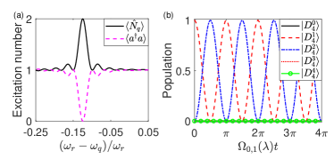
Figure 4: One-atom-excitation selective interactions of the Dicke-stark model with initial state $|D_{4}^{1}\rangle\otimes|1\rangle$. (a) After a time period $T_{2}=\pi/(2\Omega_{0,1}(\lambda))$, we plot the average number of excitations for different ratios of $(\omega_{r}-\omega_{q})/\omega_{r}$ with initial state $|D_{4}^{1}\rangle\otimes|1\rangle$, where the TC transition peaks appear for $(\omega_{r}-\omega_{q})/\omega_{r}=-0.125$ which corresponds to $\delta_{n_{0}=0,k_{0}=1}^{-}=0$; (b) The population of Dicke states with initial state $|D_{4}^{1}\rangle$, and resonance frequency locate at $(\omega_{r}-\omega_{q})/\omega_{r}=-0.125$. The other parameters are given as follows: $\omega_{r}=1$, $\lambda/\omega_{r}=0.006$ and $U/\omega_{r}=-0.5$.

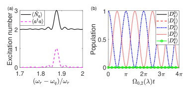
Figure 5: One-atom-excitation selective interactions of the Dicke-stark model with initial state $|D_{4}^{2}\rangle\otimes|0\rangle$. (a) After a time period $T_{3}=\pi/(2\Omega_{0,2}(\lambda))$, we plot the average excitation of the particles for different ratios of $(\omega_{r}-\omega_{q})/\omega_{r}$, where the anti-TC peaks appear at $(\omega_{r}-\omega_{q})/\omega_{r}=1.875$ which corresponds to $\delta_{n_{0}=0,k_{0}=2}^{+}=0$; (b) The population of Dicke states as a function of evolution time. The resonance frequency locate at $(\omega_{r}-\omega_{q})/\omega_{r}=1.875$. The other parameters are given as follows: $\omega_{r}=1$, $\lambda/\omega_{r}=0.006$ and $U/\omega_{r}=-0.5$.

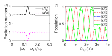
Figure 6: One-atom-excitation selective interactions of the DS model with initial states $|D_{4}^{3}\rangle\otimes|1\rangle$. (a) After a time $T_{4}=\pi/(2\Omega_{0,3}(\lambda))$, we calculation the average excitation of the particles for different ratios of $(\omega_{r}-\omega_{q})/\omega_{r}$ and initial state $|D_{4}^{3}\rangle\otimes|1\rangle$, where the TC peaks appears for $(\omega_{r}-\omega_{q})/\omega_{r}=0.125$ which corresponds to $\delta_{n_{0}=0,k_{0}=3}^{-}=0$; (b) The population of Dicke states with initial state $|D_{4}^{3}\rangle$, and resonance frequency locate at $(\omega_{r}-\omega_{q})/\omega_{r}=0.125$. The other parameters are given as follows: $\omega_{r}=1$, $\lambda/\omega_{r}=0.006$ and $U/\omega_{r}=-0.5$.

III.2 Generation GHZ state with selective TC and anti-TC model

The Greenberger-Horne-Zeilinger (GHZ) states, which can be viewed as superposition Dicke states, play very important role in several protocols of quantum communication and cryptography Greenberger et al. (1989). Here we will show how to generate GHZ state with selective two-atom excitation TC and anti-TC model. The $N$ qubits GHZ state reads

$$|GHZ\rangle_{N}=\frac{1}{\sqrt{2}}\left(|g_{1}g_{2}\cdots g_{N}\rangle+e^{i\varphi}|e_{1}e_{2}\cdots e_{N}\rangle\right).$$ (19)

Such state can be recast as superposition of Dicke states $|GHZ\rangle_{N}=\frac{1}{\sqrt{2}}\left(|D_{N}^{0}\rangle+e^{i\varphi}|D_{N}^{N}\rangle\right)$. We will show how to create four-qubit GHZ state with selective interaction. First, we prepare the initial state in $|\psi(0)\rangle=|D_{4}^{0}\rangle\otimes|0\rangle$ with $\omega_{r}=1$, $\lambda/\omega_{r}=0.1$ and $U/\omega_{r}=-16$. In Fig. 7(a), we can find the frequency near the resonant point $\tilde{\delta}_{\rm aTC}^{(2)}(0,0)=0$, and when the resonance condition is satisfied, the excitation number is 2. Tuning the resonance condition $\tilde{\delta}_{\rm aTC}^{(2)}(0,0)=0$ and applying the selective two atoms anti-TC interaction in Eq. (18) on the initial state for a time period $t_{1}=\pi/(4\Omega_{\rm aTC}^{(2)}(0,0,\lambda))$. In Fig. 7(b), we obtain

$$|\psi(t_{1})\rangle=\frac{1}{\sqrt{2}}\left(|D_{4}^{0}\rangle\otimes|0\rangle-i|D_{4}^{2}\rangle\otimes|2\rangle\right)$$ (20)

In Fig. 7(b), We can see that when the resonance frequency is satisfied, only the pre-selected subspace will oscillate periodically, while the other quantum states will not change. Then we tuning $\omega_{q}$ to satisfy the resonance condition $\tilde{\delta}_{\rm TC}^{(2)}(0,2)=0$ in Fig. 8(a), and applying the selective two atoms TC interaction in Eq. (17) on the initial state. As can be seen from Fig. 8(b), the selective interaction evaluates the state $|D_{4}^{2}\rangle\otimes|2\rangle$ to superposition between $|D_{4}^{2}\rangle\otimes|2\rangle$ and $|D_{4}^{4}\rangle\otimes|0\rangle$, but remains the state $|D_{4}^{0}\rangle\otimes|0\rangle$. At time $t_{2}=t_{1}+\pi/(2\Omega_{\rm TC}^{(2)}(0,2,\lambda))$, the evolved state reads

$$|\psi(t_{2})\rangle=\frac{1}{\sqrt{2}}\left(|D_{4}^{0}\rangle-|D_{4}^{4}\rangle\right)\otimes|0\rangle=|GHZ\rangle_{4}\otimes|0\rangle$$ (21)

Then we obtained the four qubit GHZ state in two steps. To assess the performance of this proposal, we have simulated the final states via two steps numerically, and the final state denoted by $|\psi_{f}(t_{2})\rangle$. Then we compared the final state with the target state $|\psi(t_{2})\rangle$. The fidelity of these two states is $F=|\langle\psi_{f}(t_{2})|\psi(t_{2})\rangle|^{2}=0.9952$. To obtain higher fidelity of final state, more strongly nonlinear strength is needed. We also can generate other superposition of Dicke states by tuning the qubit frequency and controlling the evolution time. In Figs. 7 and 8, we present the average excitation number and the population of Dicke states with the parameters $\omega_{r}=1$, $\lambda/\omega_{r}=0.1$ and $U/\omega_{r}=-16$.

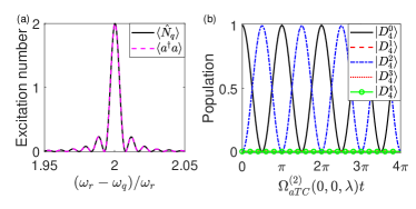
Figure 7: Two-atom-excitation selective interactions of the Dicke-stark model with initial states $|D_{4}^{0}\rangle\otimes|0\rangle$. (a) After a time $t_{1}=\pi/(2\Omega_{\rm aTC}^{(2)}(0,0,\lambda))$, we calculation the average excitation of the particles for different ratios of $(\omega_{r}-\omega_{q})/\omega_{r}$, where the anti-TC peaks appears for $(\omega_{r}-\omega_{q})/\omega_{r}=2.0003$ which corresponds to $\tilde{\delta}_{\rm aTC}^{(2)}(0,0)=0$; (b)The population of Dicke states as a function of evolution time. The resonance frequency is chosen as $(\omega_{r}-\omega_{q})/\omega_{r}=2.0003$. The other parameters are given as follows: $\omega_{r}=1$, $\lambda/\omega_{r}=0.1$ and $U/\omega_{r}=-16$.

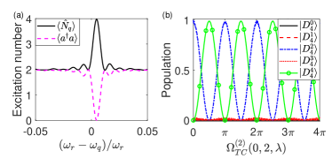
Figure 8: Two-atom-excitation selective interactions of the Dicke-stark model. (a) After a time $t_{2}-t_{1}=\pi/(2\Omega_{\rm TC}^{(2)}(0,2,\lambda))$, we calculation the average excitation of the particles for different ratios of $(\omega_{r}-\omega_{q})/\omega_{r}$ and initial state $|D_{4}^{2}\rangle\otimes|2\rangle$, where the TC peaks appears for $(\omega_{r}-\omega_{q})/\omega_{r}=0.0046$ which corresponds to $\tilde{\delta}_{\rm TC}^{(2)}(0,2)=0$; (b)The population of Dicke states with initial state $|D_{4}^{2}\rangle$, and resonance frequency is selected as $(\omega_{r}-\omega_{q})/\omega_{r}=0.0046$. The other parameters are given as follows: $\omega_{r}=1$, $\lambda/\omega_{r}=0.1$ and $U/\omega_{r}=-16$.

IV Conclusion

To summarize, we have studied the selective TC and anti-TC interaction can be engineered by means of Dicke model with Stark term. In particular, we show the selective interaction of one atomic and two atomic excitations. Their resonance conditions and oscillation frequencies depend on the number of excited atoms and the number of excited photons. In the pre-selected subspace, we can choose appropriate parameters to create selective interactions. Then we can achieve the preparation of the target state, the main process is accomplished according to RWA. With the aid of numerical simulations, we verified the correctness of the theory and successfully prepared Dicke states with very high fidelity and GHZ states which using high-order effective Hamiltonian.

References

• Horodecki et al. (2009) Ryszard Horodecki, Paweł Horodecki, Michał Horodecki,  and Karol Horodecki, “Quantum entanglement,” Rev. Mod. Phys. 81, 865–942 (2009).
• Greenberger et al. (1989) D. M. Greenberger, M. A. Horne,  and A. Zeilinger, “Bell’s theorem, quantum theory, and conceptions of the universe,” in Going Beyond Bell’s Theorem, edited by M. Kafatos (Kluwer, Dordrecht, 1989) pp. 69–72.
• Pan et al. (2012) Jian-Wei Pan, Zeng-Bing Chen, Chao-Yang Lu, Harald Weinfurter, Anton Zeilinger,  and Marek Żukowski, “Multiphoton entanglement and interferometry,” Rev. Mod. Phys. 84, 777–838 (2012).
• Dür et al. (2000) W. Dür, G. Vidal,  and J. I. Cirac, “Three qubits can be entangled in two inequivalent ways,” Phys. Rev. A 62, 062314 (2000).
• Briegel et al. (2009) H. J. Briegel, D. E. Browne, W. Dür, R. Raussendorf,  and M. Van den Nest, “Measurement-based quantum computation,” Nature Physics 5, 19–26 (2009).
• Nielsen and Chuang (2010) M. A. Nielsen and I. L. Chuang, Quantum Computation and Quantum Information (Cambridge University, Cambridge, 2010).
• Bennett et al. (1993) Charles H. Bennett, Gilles Brassard, Claude Crépeau, Richard Jozsa, Asher Peres,  and William K. Wootters, “Teleporting an unknown quantum state via dual classical and einstein-podolsky-rosen channels,” Phys. Rev. Lett. 70, 1895–1899 (1993).
• Bennett and Wiesner (1992) Charles H. Bennett and Stephen J. Wiesner, “Communication via one- and two-particle operators on einstein-podolsky-rosen states,” Phys. Rev. Lett. 69, 2881–2884 (1992).
• Ekert (1991) Artur K. Ekert, “Quantum cryptography based on bell’s theorem,” Phys. Rev. Lett. 67, 661–663 (1991).
• Dicke (1954) R. H. Dicke, “Coherence in spontaneous radiation processes,” Phys. Rev. 93, 99–110 (1954).
• Stockton et al. (2004) John K. Stockton, Ramon van Handel,  and Hideo Mabuchi, “Deterministic dicke-state preparation with continuous measurement and control,” Phys. Rev. A 70, 022106 (2004).
• Masson and Parkins (2019) Stuart J. Masson and Scott Parkins, “Extreme spin squeezing in the steady state of a generalized dicke model,” Phys. Rev. A 99, 023822 (2019).
• Wu et al. (2017) Chunfeng Wu, Chu Guo, Yimin Wang, Gangcheng Wang, Xun-Li Feng,  and Jing-Ling Chen, “Generation of dicke states in the ultrastrong-coupling regime of circuit qed systems,” Phys. Rev. A 95, 013845 (2017).
• Prevedel et al. (2009) R. Prevedel, G. Cronenberg, M. S. Tame, M. Paternostro, P. Walther, M. S. Kim,  and A. Zeilinger, “Experimental realization of dicke states of up to six qubits for multiparty quantum networking,” Phys. Rev. Lett. 103, 020503 (2009).
• Shao et al. (2010) Xiao-Qiang Shao, Li Chen, Shou Zhang, Yong-Fang Zhao,  and Kyu-Hwang Yeon, “Deterministic generation of arbitrary multi-atom symmetric dicke states by a combination of quantum zeno dynamics and adiabatic passage,” EPL (Europhysics Letters) 90, 50003 (2010).
• Cirac et al. (1994) J. I. Cirac, R. Blatt,  and P. Zoller, “Nonclassical states of motion in a three-dimensional ion trap by adiabatic passage,” Phys. Rev. A 49, R3174–R3177 (1994).
• Unanyan and Fleischhauer (2003) R. G. Unanyan and M. Fleischhauer, “Decoherence-free generation of many-particle entanglement by adiabatic ground-state transitions,” Phys. Rev. Lett. 90, 133601 (2003).
• Kasture (2018) Sachin Kasture, “Scalable approach to generation of large symmetric dicke states,” Phys. Rev. A 97, 043862 (2018).
• Hong and Lee (2002) Jongcheol Hong and Hai-Woong Lee, “Quasideterministic generation of entangled atoms in a cavity,” Phys. Rev. Lett. 89, 237901 (2002).
• Xiao et al. (2005) Yun-Feng Xiao, Zheng-Fu Han, Jie Gao,  and Guang-Can Guo, “Generation of multi-atom dicke states through the detection of cavity decay,” Journal of Physics B: Atomic, Molecular and Optical Physics 39, 485–491 (2005).
• Yu et al. (2003) Bo Yu, Zheng-Wei Zhou,  and Guang-Can Guo, “The generation of multi-atom entanglement via the detection of cavity decay,” Journal of Optics B: Quantum and Semiclassical Optics 6, 86–90 (2003).
• Ran et al. (2018) D. Ran, W. Shan, Z. Shi, Z. Yang, J. Song,  and Y. Xia, “High fidelity dicke-state generation with lyapunov control in circuit qed system,” Annals of Physics 396, 44–55 (2018).
• Solano et al. (2001) E. Solano, França M. Santos,  and P. Milman, “Quantum gates with a selective interaction,” in Modern Challenges in Quantum Optics, edited by Miguel Orszag and Juan Carlos Retamal (Springer Berlin Heidelberg, Berlin, Heidelberg, 2001) pp. 389–393.
• Solano et al. (2000) E. Solano, P. Milman, R. L. de Matos Filho,  and N. Zagury, “Manipulating motional states by selective vibronic interaction in two trapped ions,” Phys. Rev. A 62, 021401 (2000).
• Cong et al. (2020) L. Cong, S. Felicetti, J. Casanova, L. Lamata, E. Solano,  and I. Arrazola, “Selective interactions in the quantum rabi model,” Phys. Rev. A 101, 032350 (2020).
• Grimsmo and Parkins (2013a) Arne L. Grimsmo and Scott Parkins, “Cavity-qed simulation of qubit-oscillator dynamics in the ultrastrong-coupling regime,” Phys. Rev. A 87, 033814 (2013a).
• Grimsmo and Parkins (2014) Arne L. Grimsmo and Scott Parkins, “Open rabi model with ultrastrong coupling plus large dispersive-type nonlinearity: Nonclassical light via a tailored degeneracy,” Phys. Rev. A 89, 033802 (2014).
• Eckle and Johannesson (2017) Hans-Peter Eckle and Henrik Johannesson, “A generalization of the quantum rabi model: exact solution and spectral structure,” Journal of Physics A: Mathematical and Theoretical 50, 294004 (2017).
• Maciejewski et al. (2015) Andrzej J. Maciejewski, Maria Przybylska,  and Tomasz Stachowiak, “An exactly solvable system from quantum optics,” Physics Letters A 379, 1503 – 1509 (2015).
• Xie et al. (2019) You-Fei Xie, Liwei Duan,  and Qing-Hu Chen, “Quantum rabi–stark model: solutions and exotic energy spectra,” Journal of Physics A: Mathematical and Theoretical 52, 245304 (2019).
• Xie and Chen (2019) You-Fei Xie and Qing-Hu Chen, “Exact solutions to the quantum rabi-stark model within tunable coherent states,” Communications in Theoretical Physics 71, 623 (2019).
• Garraway (2011) B.M. Garraway, “The dicke model in quantum optics: Dicke model revisited,” Philosophical Transactions of the Royal Society A: Mathematical, Physical and Engineering Sciences 369, 1137–1155 (2011).
• Gopalakrishnan et al. (2011) Sarang Gopalakrishnan, Benjamin Lev,  and Paul Goldbart, “Frustration and glassiness in spin models with cavity-mediated interactions,” Phy. Rev. lett. 107, 277201 (2011).
• Bastidas et al. (2012) V. M. Bastidas, C. Emary, B. Regler,  and T. Brandes, “Nonequilibrium quantum phase transitions in the dicke model,” Phys. Rev. Lett. 108, 043003 (2012).
• Abdel-Rady et al. (2017) A. Abdel-Rady, Samia Hassan, Abdel-Nasser Osman,  and Ahmed Salah, “Quantum phase transition and berry phase of the dicke model in the presence of the stark-shift,” International Journal of Modern Physics B 31, 1750091 (2017).
• Kirton et al. (2019) Peter Kirton, Mor M. Roses, Jonathan Keeling,  and Emanuele G. Dalla Torre, “Introduction to the dicke model: From equilibrium to nonequilibrium, and vice versa,” Advanced Quantum Technologies 2, 1800043 (2019).
• Bhaseen et al. (2012) M. J. Bhaseen, J. Mayoh, B. D. Simons,  and J. Keeling, “Dynamics of nonequilibrium dicke models,” Phys. Rev. A 85, 013817 (2012).
• Dimer et al. (2007) F. Dimer, B. Estienne, A. S. Parkins,  and H. J. Carmichael, “Proposed realization of the dicke-model quantum phase transition in an optical cavity qed system,” Phys. Rev. A 75, 013804 (2007).
• Grimsmo and Parkins (2013b) A L Grimsmo and A S Parkins, “Dissipative dicke model with nonlinear atom–photon interaction,” Journal of Physics B: Atomic, Molecular and Optical Physics 46, 224012 (2013b).
• Zhang et al. (2018) Zhiqiang Zhang, Chern Hui Lee, Ravi Kumar, K. J. Arnold, Stuart J. Masson, A. L. Grimsmo, A. S. Parkins,  and M. D. Barrett, “Dicke-model simulation via cavity-assisted raman transitions,” Phys. Rev. A 97, 043858 (2018).
• Tavis and Cummings (1968) Michael Tavis and Frederick W. Cummings, “Exact Solution for an N-Molecule-Radiation-Field Hamiltonian,” Phys. Rev. 170, 379–384 (1968).
• Günter et al. (2009) G. Günter, A.A. Anappara, J. Hees, A. Sell, G. Biasiol, L. Sorba, S. De Liberato, C. Ciuti, A. Tredicucci, A. Leitenstorfer,  and R. Huber, “Sub-cycle switch-on of ultrastrong light-matter interaction,” Nature 458, 178–181 (2009).
• Niemczyk et al. (2010) T. Niemczyk, F. Deppe, H. Huebl, E.P. Menzel, F. Hocke, M.J. Schwarz, J.J. Garcia-Ripoll, D. Zueco, T. Hümmer, E. Solano, A. Marx,  and R. Gross, “Circuit quantum electrodynamics in the ultrastrong-coupling regime,” Nature Physics 6, 772–776 (2010).
• Rossatto et al. (2017) Daniel Z. Rossatto, Celso J. Villas-Bôas, Mikel Sanz,  and Enrique Solano, “Spectral classification of coupling regimes in the quantum rabi model,” Phys. Rev. A 96, 013849 (2017).
• Frisk Kockum et al. (2019) A. Frisk Kockum, A. Miranowicz, S. De Liberato, S. Savasta,  and F. Nori, “Ultrastrong coupling between light and matter,” Nature Reviews Physics 1, 19–40 (2019).
• Forn-Díaz et al. (2019) P. Forn-Díaz, L. Lamata, E. Rico, J. Kono,  and E. Solano, “Ultrastrong coupling regimes of light-matter interaction,” Rev. Mod. Phys. 91, 025005 (2019).
• Noguchi et al. (2012) Atsushi Noguchi, Kenji Toyoda,  and Shinji Urabe, “Generation of dicke states with phonon-mediated multilevel stimulated raman adiabatic passage,” Phys. Rev. Lett. 109, 260502 (2012).
• Zhou et al. (2011) Jing Zhou, Yong Hu, Xu-Bo Zou,  and Guang-Can Guo, “Ground-state preparation of arbitrarily multipartite dicke states in the one-dimensional ferromagnetic spin-$\frac{1}{2}$ chain,” Phys. Rev. A 84, 042324 (2011).
• Hume et al. (2009) D. B. Hume, C. W. Chou, T. Rosenband,  and D. J. Wineland, “Preparation of dicke states in an ion chain,” Phys. Rev. A 80, 052302 (2009).
• Huang et al. (2017) Jin-Feng Huang, Jie-Qiao Liao, Lin Tian,  and Le-Man Kuang, “Manipulating counter-rotating interactions in the quantum rabi model via modulation of the transition frequency of the two-level system,” Phys. Rev. A 96, 043849 (2017).
• Shao et al. (2017) Wenjun Shao, Chunfeng Wu,  and Xun-Li Feng, “Generalized james’ effective hamiltonian method,” Phys. Rev. A 95, 032124 (2017).
• James and Jerke (2007) D F James and J Jerke, “Effective hamiltonian theory and its applications in quantum information,” Canadian Journal of Physics 85, 625–632 (2007).