Active Learning for Deep Gaussian Process Surrogates

Abstract

Deep Gaussian processes (DGPs) are increasingly popular as predictive models in machine learning (ML) for their non-stationary flexibility and ability to cope with abrupt regime changes in training data. Here we explore DGPs as surrogates for computer simulation experiments whose response surfaces exhibit similar characteristics. In particular, we transport a DGP’s automatic warping of the input space and full uncertainty quantification (UQ), via a novel elliptical slice sampling (ESS) Bayesian posterior inferential scheme, through to active learning (AL) strategies that distribute runs non-uniformly in the input space – something an ordinary (stationary) GP could not do. Building up the design sequentially in this way allows smaller training sets, limiting both expensive evaluation of the simulator code and mitigating cubic costs of DGP inference. When training data sizes are kept small through careful acquisition, and with parsimonious layout of latent layers, the framework can be both effective and computationally tractable. Our methods are illustrated on simulation data and two real computer experiments of varying input dimensionality. We provide an open source implementation in the deepgp package on CRAN.

Keywords: sequential design, elliptical slice sampling, kriging, computer model, emulator

1 Introduction

Computer experiments are common when field data/physical measurement is scarce or non-existent. Examples include interactions in economic systems (Deissenberg et al.,, 2009), movement of satellites in low-Earth orbit (Mehta et al.,, 2014), and dispersion of diseases through populations (Fadikar et al.,, 2018). Simulation can provide insight into complex processes that might otherwise be immeasurable, but it may come with high computational costs (some runs taking days to produce output for a single input). In these cases, a surrogate model may be fit from a limited, carefully designed simulation campaign. If predictive evaluations from the surrogate are fast enough, and come with appropriate acknowledgment of uncertainty, they may be valuable as replacements for actual simulations at untried input settings. The canonical surrogate is based on Gaussian processes (GPs).

GPs are favored for their partially analytic inference and nonlinear predictive capability, including closed form variance calculations, which can be used to drive active learning (AL): the sequential design and build-up of a surrogate through a virtuous cycle of data acquisition and fitting. See texts from Santner et al., (2018), Rasmussen and Williams, (2005), and Gramacy, (2020) for a thorough review. Despite their popularity, the typical assumption of stationarity – made primarily for computational convenience – compromises the GP’s ability to accommodate features common to many computer simulations, such as regime changes in input–output dynamics. Early solutions to this problem from the spatial statistics (e.g., Sampson and Guttorp,, 1992; Higdon et al.,, 1999; Paciorek and Schervish,, 2003; Schmidt and O’Hagan,, 2003) and machine learning (ML)  perspective (e.g., Rasmussen,, 2000; Rasmussen and Ghahramani,, 2002) focused on low input dimension (e.g., longitude and latitude) and small training data sizes.

More recent advances in non-stationary spatial modeling (e.g., Bornn et al.,, 2012; Katzfuss,, 2013) emphasize scaling-up to larger training data sets, still privileging low-dimensional input spaces. The computer surrogate modeling literature now has bespoke solutions which work well in specific, modest-dimensional cases: tree–GP hybrids for when non-stationarity manifests along coordinate directions (Gramacy and Lee,, 2008); composite processes when it arises as changes in amplitudes (Ba and Joseph,, 2012); local data subsets when training data are massive (e.g., Gramacy and Apley,, 2015; Cole et al.,, 2021). Yet general purpose design and modeling strategies for an expensive, limited simulation campaign remain elusive.

We see promise in the form of deep GPs, first proposed in the ML literature by Damianou and Lawrence, (2013). The setup neatly synthesizes elements of warping, latent inputs, and composition as earlier introduced in isolation by authors of several of the papers cited above. By warping the input space through hidden Gaussian layers, effectively moving some training samples closer and others farther apart, they achieve non-stationarity even under otherwise conventional kernel structures. Prowess has been demonstrated on many classification tasks (Damianou and Lawrence,, 2013; Fei et al.,, 2018; Yang and Klabjan,, 2020). Application as surrogates for simulation experiments is rather less well developed (Radaideh and Kozlowski,, 2020).

The form of the DGP likelihood makes direct inference impossible. Initial schemes leveraged approximate variational inference (Damianou and Lawrence,, 2013), embracing computational thrift at the cost of full UQ. Recent advancements from ML, including expectation propagation (Bui et al.,, 2016), doubly stochastic variational inference (Salimbeni and Deisenroth,, 2017), and stochastic gradient Hamiltonian Monte Carlo (Havasi et al.,, 2018), perform well when data is abundant. This is a mismatch to typical surrogate modeling scenarios in which efforts to limit expensive campaigns require careful, uncertainty-driven sequential design. We thus depart from the canonical inferential apparatus to favor Markov chain Monte Carlo (MCMC) posterior sampling via a novel hybrid Gibbs–Metropolis and elliptical slice sampling (ESS; Murray et al.,, 2010) scheme. This is more expensive, but adds value in straightforward implementation and remains tractable in typical surrogate modeling scenarios. Our main goal in this paper is to demonstrate, and provide details for, effective application of DGP surrogates and AL for simulation experiments.

Some inroads have been made along these lines. Dutordoir et al., (2017) fit DGPs to sequentially collected data, but acquisition criteria were not based on the DGP fits. Rajaram et al., (2021) suggested a maximum variance criterion, a strategy sometimes called “active learning MacKay” (ALM; MacKay,, 1992), with DGPs. ALM is under-powered compared to aggregate variance-based criteria that are more common in the computer experiments literature. We propose using integrated mean-squared error (IMSE) and its ML cousin “active learning Cohn” (ALC; Cohn,, 1994), which has better properties and empirical performance under GPs (Seo et al.,, 2000; Gramacy and Lee,, 2009). Hebbal et al., (2021) applied DGPs to Bayesian optimization (BO) via expected improvement (Jones et al.,, 1998), an extension we defer to future work.

The crux of the value of our contribution lies in combining the right DGP model specification with an appropriate inferential scheme from the perspective of UQ and AL for sequential design. We advocate for a simple, limited DGP apparatus in terms of number of layers/dimensionality, and demonstrate that such setups outperform both ordinary GPs and deeper/more complex DGPs on benchmark and real-data surrogate modeling and design exercises. We furnish an R package called deepgp on CRAN, implementing every feature discussed in this manuscript. Code for all examples resides in a public git repository (https://bitbucket.org/gramacylab/deepgp-ex/).

The remainder of the paper is outlined as follows. Section 2 reviews GPs, sequential design/AL criteria, and DGPs. Section 3 details our proposed modeling template and hybrid Gibbs–ESS–Metropolis implementation. Section 4 extends this framework to AL through prediction and acquisition. Section 5 provides extensive empirical results on simulated and real computer experiments, and Section 6 concludes with a discussion.

2 Review

Here we review elements in play in this manuscript, setting the stage for our contribution: Gaussian process (GP) surrogate modeling, active learning (AL) or sequential design, and deep GPs (DGPs).

2.1 Gaussian process surrogates

We regard an expensive computer simulation as an evaluation of a blackbox function $f:\mathbb{R}^{d}\rightarrow\mathbb{R}$. To help manage simulation costs, it is common to develop a surrogate $\hat{f}_{n}:\mathbb{R}^{d}\rightarrow\mathbb{R}$ that approximates $f$ based on example outputs from a small set of $n$ designed inputs. Let $X_{n}$ denote an $n\times d$ training design of input locations and $Y_{n}=f(X_{n})$ denote the corresponding function evaluations. The canonical GP surrogate assumes a multivariate normal distribution (MVN) over the response,

$$Y_{n}\sim\mathcal{N}_{n}\left(\mu,\Sigma(X_{n})\right).$$

To streamline notation, denote $\Sigma_{n}=\Sigma(X_{n})$. The mean $\mu$ may be linear in columns of $X_{n}$, but $\mu=0$ is often sufficient after centering (Santner et al.,, 2018; Gramacy,, 2020).

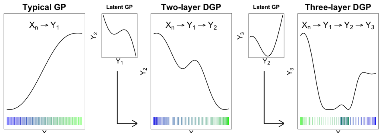
Figure 1: GP prior realization passed through latent GPs to generate two- and three-layer DGPs. Colored tick marks on the x-axes show the distribution of the latest input ($X_{n}$, $Y_{1}$, and $Y_{2}$). $Y_{1}$ clusters data at the boundaries, and $Y_{2}$ overlaps data near the middle of the input space.

The left panel of Figure 1 shows a “prior” random draw from such an MVN based on a gridded $X_{n}$ with $d=1$ under a covariance structure determined by inverse (squared) Euclidean distance:

$$\Sigma_{n}^{ij}=\tau^{2}\left(\textrm{exp}\left(-\frac{||x_{i}-x_{j}||^{2}}{\theta}\right)+g\mathbb{I}_{\{i=j\}}\right).$$ (1)

In this so-called isotropic Gaussian kernel, $\tau^{2}$, $\theta$, and $g$ act as hyperparameters controlling the scale, correlation strength (lengthscale), and noise level (nugget) respectively. We will often denote $\Sigma_{n}=\tau^{2}\left(K_{\theta}(X_{n})+g\mathbb{I}_{n}\right)$ where $K_{\theta}^{ij}=\textrm{exp}\left(-||x_{i}-x_{j}||^{2}/\theta\right)$. Our methods are largely agnostic to kernel choice. For example, a Matèrn (Stein,, 1999) would swap in nicely. We prefer an isotropic form in the DGP context, reviewed momentarily in Section 2.3, for reasons detailed later in Section 3. Extensions to so-called separable/anisotropic kernels allowing for lengthscales $\theta_{k}$ in each input direction, $k=1,\dots,d$, are preferred in typical GP regression settings.

Given (potentially noisy) training data examples $D_{n}=(X_{n},Y_{n})$, we would want to learn these hyperparameters. The MVN model structure emits the following (marginal) log likelihood,

$$\log\mathcal{L}\left(Y_{n}\mid X_{n}\right)\propto-\frac{1}{2}\log|\Sigma_{n}|-\frac{1}{2}Y_{n}^{\top}\Sigma_{n}^{-1}Y_{n}.$$ (2)

Maximum likelihood estimates are commonly used as plug-ins for $\tau^{2}$, $\theta$, and $g$. MLE $\hat{\tau}^{2}$ has a closed form. Derivative-based numerical maximization is required for $\hat{\theta}$ and $\hat{g}$. Details and implementation are provided by Gramacy, (e.g., 2020, Chapter 5). Here we promote Bayesian posterior sampling, thinking ahead to DGPs. One can marginalize $\tau^{2}$ out of the posterior analytically under a reference prior ($\pi(\tau^{2})\propto 1/\tau^{2}$), or any conditionally conjugate inverse Gamma specification; however, $\theta$ and $g$ require rejection-based MCMC schemes (i.e., Metropolis–Hastings). Details are provided, e.g., by Gramacy, (2020, Section 5.5). When training data sizes are low, it can be crucial to average over posterior uncertainty for $\theta$ and $g$ which, together, facilitate a signal-to-noise trade-off.

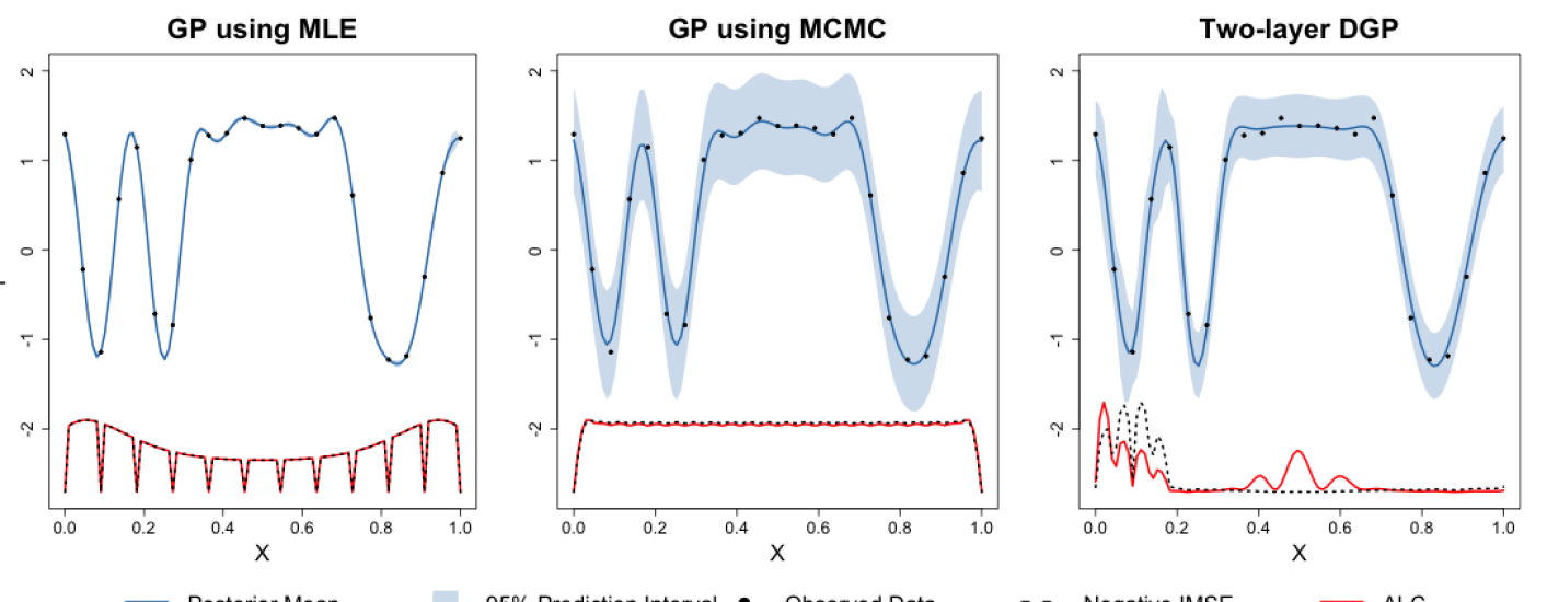
Figure 2: Surrogates $\hat{f}_{n}$ fit to data from $f(x)$ in Eq. (20): (left) using MLE $\hat{g}$ and $\hat{\theta}$; (center) using MCMC sampling of $g$ and $\theta$; (right) using a two-layer DGP (described in Section 3). ALC and IMSE (negated in order to maximize) are plotted along a dense grid of candidate locations.

Given $D_{n}$, and under settings of hyperparameters (either MLE or via posterior sampling), the posterior predictive distribution for an $n^{\prime}\times d$ matrix of testing locations $\mathcal{X}$ has closed form

$$Y(\mathcal{X})\mid D_{n} \sim\mathcal{N}_{n^{\prime}}\left(\mu_{Y}(\mathcal{X}),\Sigma_{Y}(\mathcal{X})\right), \mbox{where }\quad\mu_{Y}(\mathcal{X}) =\Sigma(\mathcal{X},X_{n})\Sigma_{n}^{-1}Y_{n}$$ (3)

$$\Sigma_{Y}(\mathcal{X}) =\Sigma(\mathcal{X})-\Sigma(\mathcal{X},X_{n})\Sigma_{n}^{-1}\Sigma(X_{n},\mathcal{X}),$$

and $\Sigma(X_{n},\mathcal{X})$ is an $n\times n^{\prime}$ matrix derived by extending the kernel across training and testing elements. These equations, coupled with an inferential strategy (e.g., MLE $\hat{\tau}^{2}$ converts Gaussian to Student-$t$), complete the description of surrogate $\hat{f}_{n}$. A 1d illustration is provided in the left and center panels of Figure 2, based on MLE and full posterior sampling, respectively. The GP surrogate’s flexibility provides accurate posterior mean estimates in the non-linear regions, but MLE point-estimates (left) lead to over-fitting – interpreting noise as signal – in the flat region. Full posterior sampling (center) appropriately averages over posterior evidence for both regimes.

The conditionally analytic structure of GP prediction (3) is convenient, and its UQ capability – particularly via MCMC as in the middle panel of Figure 2 – supports a wide range of downstream applications such as Bayesian optimization (Jones et al.,, 1998; Picheny et al.,, 2016), computer model calibration to field data (Kennedy and O’Hagan,, 2001; Higdon et al.,, 2004), and input sensitivity analysis (Saltelli,, 2002; Oakley and O’Hagan,, 2004; Marrel et al.,, 2009). But GPs are no panacea. Working with MVNs involves dense $n\times n$ matrices, requiring quadratic-in-$n$ storage and cubic decomposition. Meanwhile, covariance based solely on relative (inverse Euclidean) distance can be too rigid for dynamics involved in many simulations, limiting the GP’s ability to capture features that change positionally in the input configuration space. This so-called stationarity limitation is coupled, from a practicality perspective, with computational bottlenecks. Even if stationarity is relaxed, multiple regimes may not be recognized without large amounts of training data.

2.2 Active learning

The most common designs for computer simulation experiments are based on space-filling principles, either along the margins with Latin hypercube samples (LHSs; McKay et al.,, 2000), via pairwise distances (Johnson et al.,, 1990), or hybrids thereof (Morris and Mitchell,, 1995). These are fine strategies, but they presume a fixed budget of $n$ runs in advance. Sequential adaptations exist but do not leverage model uncertainties. For a review, see Gramacy, (2020, Chapter 4). Model-based analogues, which devise criteria via prior–posterior information gain (so-called maximum entropy designs; Shewry and Wynn,, 1987) and posterior mean-squared prediction error (MSE), offer similar behavior. But these have a chicken-or-egg problem because they condition on (a priori unknown) hyperparameter settings. Sequential adaptations, suitably initialized (Zhang et al.,, 2021), offer a natural remedy. See Gramacy, (2020, Chapter 6).

Much recent work on sequential design for GPs comes from ML as a branch of reinforcement learning called active learning (AL). We adopt their terminology of solving acquisition functions (sequential design criteria) to “actively” select the data which the model is trained on: begin (0) with a small training data set $D_{n}=(X_{n},Y_{n})$ of size $n=n_{0}$; then (1) fit a flexible model to $D_{n}$; and (2) select $x_{n+1}$ to augment the data $n\rightarrow n+1$; and (3) repeat from (1). This setup avoids many pathologies inherent to static/batch training through a baby-steps approach and allows progress to be monitored. Maximum-variance acquisitions (for step 2) were shown to approximate maximum entropy designs without the burden of setting unknown hyperparameters (MacKay,, 1992). Aggregate variance-based acquisitions (Cohn,, 1994) approximately minimized MSE. Both ideas were originally for neural networks (step 1), but were subsequently ported to GPs (Seo et al.,, 2000). Acquisition based on expected improvement could target minima in blackbox simulation output (e.g., Snoek et al.,, 2012; Picheny et al.,, 2016; Gramacy,, 2020, Chapter 7).

Here we emphasize building up a simulation campaign where runs are acquired to reduce MSE. Let $X_{n+1}=\{x_{1},\dots,x_{n},x_{n+1}\}$ represent the combined set of $n$ current input locations and new input location $x_{n+1}$. Let $\sigma^{2}_{n}(x)$ denote the posterior predictive variance (i.e., the MSE) at location $x$ calculated from $X_{n}$, i.e., via Eq. (3) with singleton $\mathcal{X}=\{x\}$. Take hyperparameter settings from MLE calculations or as posterior samples conditioned on data $D_{n}$. Now, let $\breve{\sigma}^{2}_{n+1}(x)$ denote the deduced posterior predictive variance at location $x$ calculated from the augmented $X_{n+1}$, but otherwise with hyperparameter settings based on $D_{n}$.

$$\breve{\sigma}_{n+1}^{2}(x)=\Sigma(x)-\Sigma(x,X_{n+1})\Sigma_{n+1}^{-1}\Sigma(X_{n+1},x)$$

We follow the convention of defining both $\sigma_{n}^{2}(x)$ and $\breve{\sigma}_{n+1}^{2}(x)$ for the purpose of AL via $\Sigma(x)=1$ rather than $\Sigma(x)=1+g$, targeting the variance of the latent random field (i.e., the variance of the mean) rather than the full predictive variance. Making this, and other kernel details explicit …

$$\breve{\sigma}_{n+1}^{2}(x)=\tau^{2}\left(1-K_{\theta}(x,X_{n+1})\left(K_{\theta}(X_{n+1})+g\mathbb{I}_{n+1}\right)^{-1}K_{\theta}(X_{n+1},x)\right).$$

Hence $\breve{\sigma}_{n+1}^{2}(x)\rightarrow 0$ as $n\rightarrow\infty$, providing a natural “asymptote for learning.” Observe that the nugget $g$ is still involved in $\Sigma_{n+1}^{-1}$.

It is sensible to acquire new $x^{\star}_{n+1}$ to minimize $\breve{\sigma}_{n+1}^{2}(x)$ integrated over all $x$,

$$x_{n+1}^{\star}=\operatorname*{argmin}_{x_{n+1}}\;\textrm{IMSE}(X_{n+1})\quad\textrm{where}\quad\textrm{IMSE}(X_{n+1})=\int\breve{\sigma}_{n+1}^{2}(x)\,dx.$$

When the input space used in the domain of integration is a hyper-rectangle, a closed form expression is available. See, e.g., Binois et al., (2019) for coded inputs $[0,1]^{d}$ and extensions by Cole et al., (2021) to $[a,b]^{d}$ and Gaussian measures over inputs.

Despite a degree of analytic tractability, calculating IMSE is cumbersome, especially in the Bayesian posterior sampling context. Varying hyperparameterization thwarts many pre-calculations and matrix decomposition tricks that would otherwise lend a degree of efficiency. Instead we prefer an approximation obtained by extending Monte Carlo integration over posterior draws to include the input space. This is the acquisition criteria now known as “active learning Cohn” (ALC; Cohn,, 1994; Seo et al.,, 2000). Observe that minimizing IMSE over $x_{n+1}$ is equivalent to maximizing the difference between $\sigma^{2}_{n}(x)$ and $\breve{\sigma}^{2}_{n+1}(x)$.

$$\Delta\sigma_{n}^{2}(X_{n+1}) =\int\sigma^{2}_{n}(x)-\breve{\sigma}_{n+1}^{2}(x)dx\propto\int\tau^{2}K_{\theta}(x,X_{n+1})\left(K_{\theta}(X_{n+1})+g\mathbb{I}_{n}\right)^{-1}K_{\theta}(X_{n+1},x)dx$$

The ALC criterion approximates this integral with a sum over a reference set, $X_{\mathrm{ref}}$,

$$\textrm{ALC}(X_{n+1}\mid X_{\mathrm{ref}}) \propto\sum_{x\in X_{\mathrm{ref}}}\tau^{2}K_{\theta}(x,X_{n+1})\left(K_{\theta}(X_{n+1})+g\mathbb{I}_{n+1}\right)^{-1}K_{\theta}(X_{n+1},x)$$ (4)

with acquisition as $x_{n+1}^{\star}=\mathrm{argmax}_{x_{n+1}}\textrm{ALC}(X_{n+1}\mid X_{\mathrm{ref}})$. A uniform reference set yields proportional ALC and IMSE surfaces. See left and center panels of Figure 2. Instead of library-based optimization (Gramacy and Apley,, 2015), we prefer discrete search over (possibly random) candidates because this lends well to averaging across MCMC iterations and parallel implementation.

Even with variance-based criteria, AL is limited by the stationarity of the covariance kernel of the GP (Gramacy and Lee,, 2009). In Figure 2, the MLE surface (left) gets the “wrong answer” as regards AL, discouraging acquisition where it needs it most: in the middle of inputs where it has confused noise as signal. With MCMC (center), the ALC/IMSE criteria indentify a more uniform preference for the next run, although both ultimately prefer runs near the edges, which manifests as a form of leverage in this case. Neither MLE nor MCMC-based fits are able to recognize what human intuition would likely suggest: more data is needed where the function is wiggly than where it is not. This is not the fault of the AL criteria. The stationary GP is not “allowed” to recognize two (or more) distinct regimes, of wiggly and flat. Only after relaxing stationarity, so that predictive variance is not simply a matter of distance to nearby training values, can we obtain a notion of predictive uncertainty which is region-dependent.

2.3 Deep Gaussian processes

A DGP is a hierarchical layering of GPs where each layer is conditionally MVN. This definition is inherently broad and lends to various formulations. Dunlop et al., (2018) detailed four methods for constructing DGPs, each providing different levels of feasibility and interpretability. We view DGPs as functional compositions, arguably the most interpretable and easily implemented option.

In a DGP prior, the inputs $X_{n}$ are mapped through one or more intermediate GPs before reaching the response $Y_{n}$. The inputs to those intermediate “layers” act as latent variables, warping the input space but remaining unobserved. Henceforth, we shall refer to typical GP regression as described in Section 2.1 as a “one-layer” GP. A two-layer model, with inputs to the new hidden GP labeled as $W$, may be described hierarchically as

$$Y_{n}\mid W \sim\mathcal{N}_{n}\left(0,\Sigma(W)\right) \quad\quad W \sim\mathcal{N}_{n}\left(0,\Sigma(X_{n})\right).$$ (5)

Conditional on $\Sigma$, the marginal likelihood may be represented as an integral over unknown $W$,

$$\mathcal{L}(Y_{n}\mid X_{n})\propto\int\mathcal{L}(Y_{n}\mid W)\mathcal{L}(W\mid X_{n})\;dW$$ (6)

where $\log\mathcal{L}(Y_{n}\mid W)$ and $\log\mathcal{L}(W\mid X_{n})$ are defined as in Eq. (2). A three-layer model will have two hidden layers (denoted $Z$ and $W$) and will involve three MVN likelihoods with a double integral over $Z$ and $W$. The center and right panels of Figure 1 show the hierarchical composition of two- and three-layer DGPs in a single dimension, accumulating from the left panel’s ordinary, one-layer GP. As uniformly distributed $X_{n}$ are fed through intermediate layers they are re-distributed, and response values are no longer stationary. Intermediate layers are not confined to a single dimension. In fact, a single latent dimension is often inadequate. We will refer to multiple component dimensions of intermediate layers as “nodes”, following deep learning nomenclature.

Adding additional depth and nodes to intermediate layers will eventually yield diminishing returns. Damianou and Lawrence, (2013) found some justification for a five-layer DGP in classification tasks, but two- and three-layer DGPs have been sufficient for real-valued outputs common to computer surrogate modeling (Radaideh and Kozlowski,, 2020). Dunlop et al., (2018) similarly preferred two and three layers. We find that low numbers of latent nodes (no higher than the dimension of the input space) and limited depth (no deeper than three layers) are sufficient for surrogate modeling and AL. More details are provided in Section 3 with evidence in Section 5. The benefit of DGPs from the perspective of AL is foreshadowed in the right panel of Figure 2. A degree of nonstationarity, as facilitated by warping the input space so that some pairs are (effectively) closer than others when calculating covariance, is sufficient to nudge acquisitions towards the “interesting” part of the input space, rather than being essentially space-filling.

Closed form Bayesian inference for two- and three-layer DGPs is intractable since it is not possible to analytically integrate the hidden layer(s) out of the (marginal) likelihood (6). Variational inference and other maximization–oriented methods (Damianou and Lawrence,, 2013; Salimbeni and Deisenroth,, 2017) are computationally thrifty, but yield probabilistic representations which can over-simplify, particularly as regards UQ. MCMC methods address uncertainty more thoroughly at the expense of computation. To mitigate these costs, efficient mixing of the Markov chain is essential.

3 Modeling and inference

Here we outline a novel elliptical slice sampling-based scheme for posterior inference with DGPs.

3.1 Model specification

In a DGP, extreme flexibility can come at the cost of identifiability and practicality. Here we provide a template that has worked well for surrogate modeling in several realistic settings, as showcased in Section 5, and which supports AL efforts (Section 4). We begin with a two-layer setup (5), defining the hierarchical structure in terms of distance-based covariance (1).

$$Y_{n}\mid W \sim\mathcal{N}_{n}\left(0,\tau^{2}(K_{\theta_{y}}(W)+g\mathbb{I}_{n})\right) \quad\quad W \sim\mathcal{N}_{n}\left(0,K_{\theta_{w}}(X_{n})\right)$$ (7)

Notice that scale $\tau^{2}$ and nugget $g$ are placed on the outer layer only. Specifying noiseless hidden layers with unit scale is crucial, we find, to stable posterior inference.

Although the notation in Eq. (7) is suggestive of a one-dimensional $W$, in practice it can be beneficial to have multiple nodes, i.e., a multi-dimensional $W$. We find that $\mathrm{dim}(W)=\mathrm{dim(X_{n})}=d$ works well as a default, although smaller values may be appropriate for high-dimensional $X_{n}$. Let $W_{j}$ represent the $j^{\mathrm{th}}$ node of $W$ for $j=1,\dots,p$. Note that, like a column of $X_{n}$ or response $Y_{n}$, $W_{i}$ is an $n$-vector with one coordinate for each training data point. Although nodes of $W$ could be modeled jointly with cross covariances, we recommend the following simplifications.

• $W_{j}$ and $W_{k}$, for $j\neq k$, are conditionally independet (Damianou and Lawrence,, 2013).

• Each $W_{j}$ is modeled as isotropic (1) in inputs $X_{n}$ via unique scalar lengthscale $\theta_{w}[j]$, for $j=1,\dots,p$, regardless of the input dimension $d$.

• Similarly, $Y_{n}$ is modeled as isotropic in all nodes of $W$ with scalar lengthscale $\theta_{y}$.

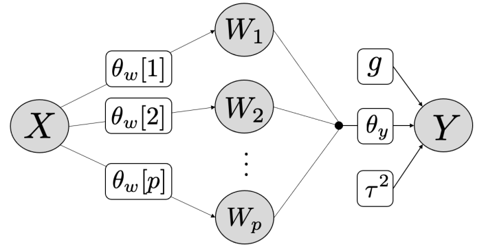
Figure 3: Model structure for a two-layer DGP with $p$ latent nodes.

Figure 3 depicts this model structure, still focusing on the two-layer setup. Impositions ii.–iii. are essential to reign in complexity. Latent $W$, even with a single node but especially for $p\gg 1$, offer more than enough flexibility to “imitate” a separable/anisotropic kernel without the added complexity of additional lengthscale parameters. This is simplest to see with $p=d$. If the data desire lower correlation in one coordinate direction compared to another, then components of $W$ can organize themselves so that $W_{j}$, say, “fans out” more than $W_{k}$ does. Of course, it is easy to imagine more complicated arrangements. The filled circle between the $W$ and $Y$ layers in the diagram represents imposition iii., depicting that all nodes of $W$ form inputs to the outer layer for $Y$ under isotropic (scalar) lengthscale $\theta_{y}$.

Building off that setup, consider a three-layer model built as follows.

$$Y_{n}\mid W \sim\mathcal{N}_{n}\left(0,\tau^{2}(K_{\theta_{y}}(W)+g\mathbb{I}_{n})\right) \quad W\mid Z \sim\mathcal{N}_{n}\left(0,K_{\theta_{w}}(Z)\right)$$

$$Z \sim\mathcal{N}_{n}\left(0,K_{\theta_{z}}(X_{n})\right)$$

Here, as above, conditional independence and isotropy (i.-ii.) for $W$ is duplicated in the new latent layer $Z$. We have found it helpful to restrict the number of nodes in $Z$ to match $W$, i.e., $\mathrm{dim}(Z)=\mathrm{dim}(W)=p\leq d$. Again, each $Z_{j}$ is an $n$-vector, for $j=1,\dots,n$, of latent variables.

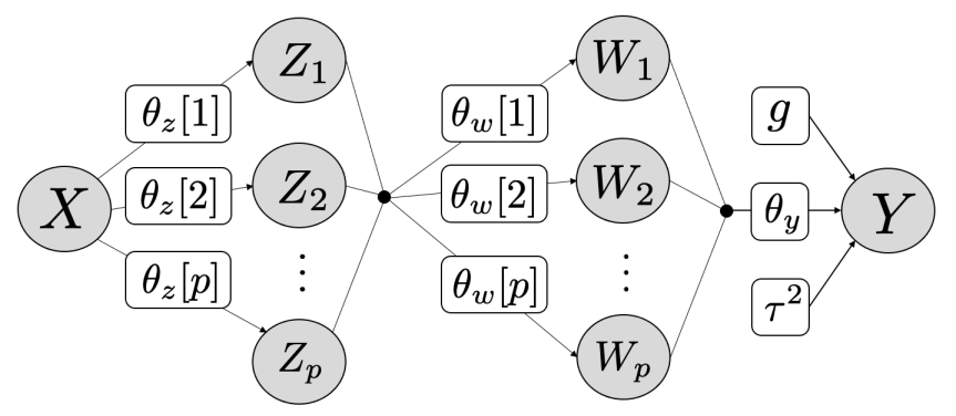
Figure 4: Model structure for a three-layer DGP with $p$ latent nodes in $Z$ and $W$.

Figure 4 depicts this structure diagrammatically. The filled circle between $Z$ and $W$ layers, with edges fanning out in both directions, is intended to represent communication between all $Z$ and $W$ nodes, like an “information bus” capturing $p^{2}$ interconnections. Each latent $Z_{j}$ input, $j=1,\dots,p$, is connected to each $W_{k}$ output through an inverse-distance-based covariance kernel with (scalar) lengthscale parameters $\theta_{w}[k]$, for $k=1,\dots,p$.

Hyperparameter priors

We complete our Bayesian hierarchical model specification with the following priors on hyperparameters, comprising lengthscales $\theta=\{\theta_{y},\theta_{w},\theta_{z}\}$, scale $\tau^{2}$, and nugget $g$ on the outer layer. Conditionally conjugate inverse Gamma (IG) priors are common for scales like $\tau^{2}$ because they may subsequently be analytically integrated out of an otherwise numerical posterior sampling scheme. Details are provided in Section 3.2 shortly. Specifying IG parameters of zero (following the description in Gelman et al.,, 2013) leads to a so-called reference prior $\pi(\tau^{2})\propto 1/\tau^{2}$ (Berger et al.,, 2001), which is a common default in GP spatial modeling. Although improper, the posterior is proper (in our zero-mean context) as long as $n\geq 1$, i.e., as long as there is at least one training data example.

We prefer proper priors for the other parameters, and choose members of the Gamma family as their familiar form offers convenient specification, which we tailor to penalize against pathological settings such as $\theta\rightarrow\{0,\infty\}$. Specifically, consider $\{\theta,g\}\stackrel{{\scriptstyle\mathrm{iid}}}{{\sim}}\mathrm{G}(3/2,b_{[\cdot]})$ where $b_{[\cdot]}$ is adjusted depending on the hyperparameter in question. This choice mirrors other work in Bayesian posterior sampling of GP hyperparameters (e.g., Gramacy and Lee,, 2008) and in penalized marginal maximum likelihood settings (e.g., Gramacy and Apley,, 2015). We find it helpful to nudge the posterior toward a hierarchy in the latent nodes with $b_{[\theta_{y}]}>b_{[\theta_{w}]}>b_{[\theta_{z}]}$ encoding a prior belief that as layers get deeper they should be less “wiggly” (closer to the identity mapping). Particular, user-adjustable, default values for $b_{[\cdot]}$ provided in our software are detailed in Section 5.1. When modeling a deterministic computer model simulation in the outer layer we fix $g=\varepsilon$, a small non-zero value such as sqrt(.Machine$double.eps) in R, to interpolate those runs.

3.2 MCMC posterior sampling

Here we propose a hybrid Gibbs–ESS–Metropolis scheme for sampling hyperparameters and latent layers. A closed form GP marginal likelihood, integrating out scale $\tau^{2}$ under the reference prior, is crucial to the subsequent development. Although the calculation is rather textbook, e.g., see Gramacy, (2020, Section 5.5, exercise 1), we provide it below in our notation for concreteness.

$$\log\mathcal{L}(Y_{n}\mid W,\theta_{y},g)\propto-\frac{n}{2}\log\left(n\hat{\tau}^{2}\right)-\frac{1}{2}\log|K_{\theta_{y}}(W)+g\mathbb{I}_{n}|\;\mbox{ with }\;\hat{\tau}^{2}=\frac{Y^{\top}(K_{\theta_{y}}(W)+g\mathbb{I}_{n})^{-1}Y}{n}$$ (8)

Throughout, relationship “$\propto$” for log likelihoods denotes that an additive constant has been dropped. Taking $W\equiv X_{n}$ lends explicit form to Eq. (2) for the ordinary GP case, where $\hat{\tau}^{2}$ may be interpreted as an MLE. For DGPs with two and three layers, we additionally need

$$\log\mathcal{L}(W\mid Z,\theta_{w}) \propto\sum_{i=1}^{p}\log\mathcal{L}\left(W_{i}\mid Z,\theta_{w}[i]\right)$$ (9)

$$\propto\sum_{i=1}^{p}\left(-\frac{1}{2}\log|K_{\theta_{w}[i]}(Z)|-\frac{1}{2}W_{i}^{\top}\left(K_{\theta_{w}[i]}(Z)\right)^{-1}W_{i}\right).$$

In two-layers, take $Z\equiv X_{n}$ and collect

$$\log\mathcal{L}(Y_{n}\mid W,X_{n},\theta,g)=\log\mathcal{L}(Y_{n}\mid W,\theta_{y},g)+\log\mathcal{L}(W\mid X_{n},\theta_{w}),$$

combining Eqs. (8–9). Of course, in the context above of unknown (latent) $W$, the quantity $\log\mathcal{L}(W\mid X_{n},\theta_{w})$ is actually a log prior, but its form is nevertheless given by Eq. (9), so we find it convenient to notate using marginal log likelihoods.

Finally, in the three layer case (with trivial extension beyond), we have

$$\log\mathcal{L}(Y_{n}\mid W,Z,X_{n},\theta,g)=\log\mathcal{L}(Y_{n}\mid W,\theta_{y},g)+\log\mathcal{L}(W\mid Z,\theta_{w})+\log\mathcal{L}(Z\mid X_{n},\theta_{z})$$

where the third term (and beyond) follows Eq. (9) for $Z$ and $X_{n}$ instead of $W$ and $Z$. The posterior distribution is completed with the hyperparameter priors outlined at the end of Section 3.1,

$$\pi(W,Z,\theta,g\mid D_{n})\propto\mathcal{L}(Y_{n}\mid W,Z,X_{n},\theta,g)\times\pi(\theta,g),$$

and the remainder of this section details how we obtain samples in the Gibbs framework summarized in Algorithm 1. Hyperparameters $\theta$ and $g$ follow a somewhat conventional random-walk Metropolis–Hastings (MH) procedure. To acknowledge a restricted support $[\varepsilon,\infty]$, proposals $(q)$ follow a “uniform sliding window” scheme first outlined by Gramacy and Lee, (2008) whereby

$$\theta^{\star}\sim\textrm{Unif}\left(\frac{\ell\theta^{(t-1)}}{u},\frac{u\theta^{(t-1)}}{\ell}\right)\quad\mbox{ so that }\quad\frac{q(\theta^{(t-1)}\mid\theta^{\star})}{q(\theta^{\star}\mid\theta^{(t-1)})}=\frac{\theta^{(t-1)}}{\theta^{\star}}$$ (10)

features as the proposal ratio in the MH acceptance probability. We sample all components of $\theta$ and $g$ (except when $g\rightarrow\varepsilon$ for interpolating deterministic simulations) in this way. Defaults for tuning parameters $u$ and $\ell$ are given in Section 5.1. Under our template, each hyperparameter is involved in only one likelihood component. Thus each MH acceptance ratio requires only one MVN density evaluation. For example, acceptance for $\theta_{y}^{\star}$ is based on

$$\alpha=\min\left(1,\frac{\mathcal{L}\left(Y_{n}\mid W,\theta_{y}^{\star},g\right)\pi\left(\theta_{y}^{\star}\right)}{\mathcal{L}\left(Y_{n}\mid W,\theta_{y}^{(t-1)},g\right)\pi\left(\theta_{y}^{(t-1)}\right)}\times\frac{\theta_{y}^{(t-1)}}{\theta_{y}^{\star}}\right).$$ (11)

The likelihood component involved in each Metropolis–within-Gibbs step is detailed in Algorithm 1. To shorten this algorithm for a two-layer model, simply remove sampling of $\theta_{z}$ and $Z$ and replace remaining instances of $Z$ with $X_{n}$.

initialize $g^{(1)}$, $\theta_{y}^{(1)},\theta_{w}^{(1)}$, $\theta_{z}^{(1)}$, $W^{(1)},$and $Z^{(1)}$

for $t=2,\dots,T$ do

       $g^{(t)}\sim\pi(g\mid Y_{n},W^{(t-1)},\theta_{y}^{(t-1)},g^{(t-1)})$

        // MH (11) via $\mathcal{L}(Y_{n}\mid W,\theta_{y}\ g)$

       $\theta_{y}^{(t)}\sim\pi(\theta_{y}\mid Y_{n},W^{(t-1)},\theta_{y}^{(t-1)},g^{(t)})$

        // MH (11) via $\mathcal{L}(Y_{n}\mid W,\theta_{y}\ g)$

       for $i=1,\dots,p$ do

             $\theta_{w}[i]^{(t)}\sim\pi(\theta_{w}[i]\mid W_{i}^{(t-1)},Z^{(t-1)},\theta_{w}[i]^{(t-1)})$

              // MH (11) via $\mathcal{L}(W_{i}\mid Z,\theta_{w}[i])$

            

      for $i=1,\dots,p$ do

             $\theta_{z}[i]^{(t)}\sim\pi(\theta_{z}[i]\mid Z_{i}^{(t-1)},X_{n},\theta_{z}[i]^{(t-1)})$

              // MH (11) via $\mathcal{L}(Z_{i}\mid X_{n},\theta_{z}[i])$

            

      for $i=1,\dots,p$ do

             $W_{i}^{(t)}\sim\pi(W\mid Y_{n},W_{\geq i}^{(t-1)},W_{<i}^{(t)},Z^{(t-1)},g^{(t)},\theta_{y}^{(t)},\theta_{w}^{(t)})$

              // ESS via (13)

            

      for $i=1,\dots,p$ do

             $Z_{i}^{(t)}\sim\pi(Z\mid X_{n},W^{(t)},Z_{\geq i}^{(t-1)},Z_{<i}^{(t)},\theta_{w}^{(t)},\theta_{z}^{(t)})$

              // ESS via (14)

            

      

Algorithm 1 Gibbs sampling procedure for three-layer DGP

Latent $W$ and $Z$ could be handled similarly, i.e., by MH. While there are a number of approaches for sampling Gaussian fields in non-conjugate settings (e.g., Neal,, 2011; Oliver et al.,, 1997; Higdon et al.,, 2003), such rejection-based samplers may mix poorly even with tedious fine tuning of proposal functions. We think this is why MCMC inference for DGPs is often dismissed in preference for maximization–based shortcuts. However, we find elliptical slice sampling (ESS; Murray et al.,, 2010) of $W$ and $Z$ to be particularly efficient.

To adapt ESS for DGP latent layers, allow us to briefly digress to the general case in which we desire samples from a posterior under a zero-mean MVN prior, $\pi(f)\propto\mathcal{L}(f)\times\mathcal{N}(f;0,\Sigma)$. ESS initializes with a random draw from the prior $f^{\mathrm{prior}}\sim\mathcal{N}(0,\Sigma)$ and a random angle $\gamma\sim\mathrm{Unif}(0,2\pi)$ with consequent boundaries set to $\gamma_{\min}=\gamma-2\pi$ and $\gamma_{\max}=\gamma$. Proposal $f^{\star}$ is a function of the previous iteration, the prior draw, and the angle,

$$f^{\star}=f^{(t-1)}\cos\gamma+f^{\mathrm{prior}}\sin\gamma\quad\mbox{with acceptance probability~{}}\quad\alpha=\min\left(1,\frac{\mathcal{L}(f^{\star})}{\mathcal{L}(f^{(t-1)})}\right).$$ (12)

Upon rejection, ESS shrinks the “bracket” on the angle – specifically, setting $\gamma_{\min}=\gamma$ if $\gamma<0$ and $\gamma_{\max}=\gamma$ otherwise – and re-samples $\gamma\sim\mathrm{Unif}(\gamma_{\min},\gamma_{\max})$, yielding new $f^{\star}$. The process is repeated, shrinking the bracket and re-proposing, until acceptance, constituting one iteration/one sample. This distinguishes ESS from MH methods in which rejections result in identically repeated values and poor mixing. Although ESS may require more likelihood evaluations (each new proposal warrants one) than MH, it tends to yield more “effective samples” (Kass et al.,, 1998) through enhanced mixing, as demonstrated in Section 3.3, all without having to set any tuning parameters.

To implement ESS for $W$ and $Z$, one may leverage the likelihood (9) as a prior over the unknown function. First generate from the prior for each node,

$$W_{i}^{\mathrm{prior}}\sim\mathcal{N}_{n}\left(0,K_{\theta_{w}[i]}(Z)\right)\quad\mbox{and}\quad Z_{i}^{\mathrm{prior}}\sim\mathcal{N}_{n}\left(0,K_{\theta_{z}[i]}(X_{n})\right)\!.$$

In the two-layer case, set $Z\equiv X_{n}$ for each $W_{i}$. ESS proposals $W_{i}^{\star}$ and $Z_{i}^{\star}$ follow Eq. (12) based on previous iteration $W_{i}^{(t-1)}$ and $Z_{i}^{(t-1)}$ respectively. Acceptance probabilities are based on a likelihood component designed to “receive” that latent quantity as an input. Even though nodes of a layer are independently proposed, all are involved in the model likelihood (under imposition iii.) and hence impact acceptance. For $W_{i}$, in either a two- or three-layer model, that involves Eq. (8),

$$\alpha=\min\left(1,\frac{\mathcal{L}(Y_{n}\mid W_{i}^{\star},W_{>i}^{(t-1)},W_{<i}^{(t)},\theta_{y},g)}{\mathcal{L}(Y_{n}\mid W_{\geq i}^{(t-1)},W_{<i}^{(t)},\theta_{y},g)}\right)$$ (13)

where, in true Gibbs fashion, we condition on the most recent iteration of each node. Acceptance probabilities for $Z_{i}$ use the likelihood of Eq. (9).

$$\alpha=\min\left(1,\frac{\mathcal{L}(W\mid Z_{i}^{\star},Z_{>i}^{(t-1)},Z_{<i}^{(t)},\theta_{w})}{\mathcal{L}(W\mid Z_{\geq i}^{(t-1)},Z_{<i}^{(t)},\theta_{w})}\right)$$ (14)

In contrast to $\theta_{w}[i]$, which only features in one component of this likelihood, acceptance of node $Z_{i}$ requires full evaluation of this likelihood (including all $p$ elements of the sum). Specific implementation details, including default priors and proposals, and demonstration of the mixing of ESS samples of latent layers are provided in Sections 5.1 and 3.3, respectively.

3.3 Illustration

MCMC sampling of latent layers $W$ and $Z$ is crucial to downstream tasks, such as AL in Section 4. Their posteriors are inherently multi-modal, since only pairwise distances feature in the next layer. Such lack of identifiability poses a challenge to MCMC mixing and posterior exploration, but on the flip side of that coin is a convenient barometer for judging a proposed sampling scheme.

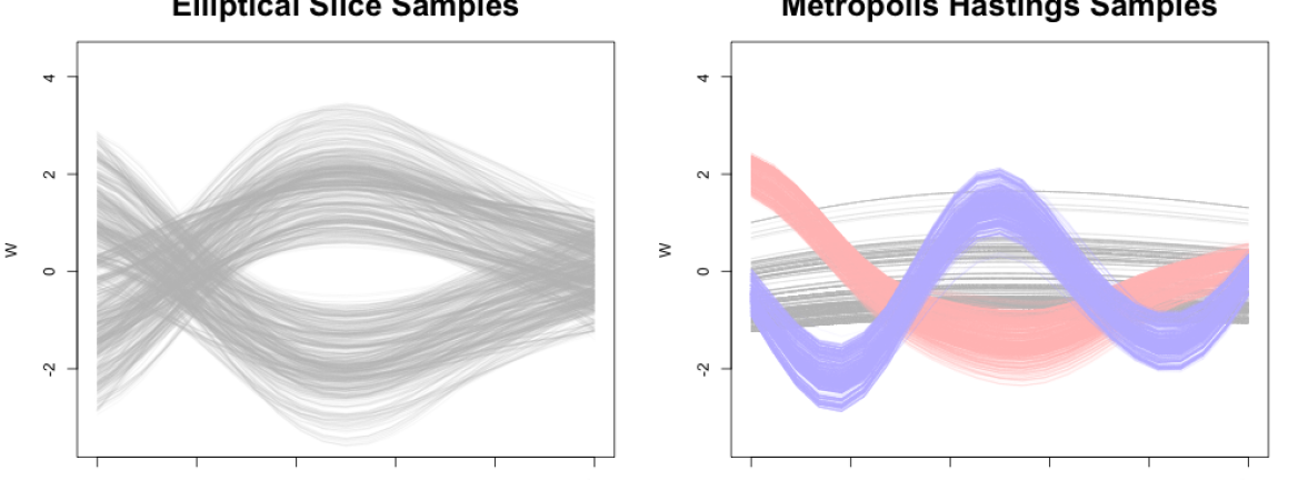
Figure 5: ESS and MH samples of latent $W$ from the two-layer DGP of Figure 2, otherwise following Algorithm 1 for hyperparameters $\theta$ and $g$. MH samples show three different initializations; each (three MH & one ESS) comprise 10,000 total and 6,000 burn-in iterations with thinning by half.

Our ESS proposal mechanism (12) is particularly well-suited for this as it can “bounce” back and forth between modes. To demonstrate, consider the setup in Figure 2 with a two-layer DGP. The fitted surface is shown in the right panel, but we have not yet discussed prediction (Section 4.1). For now, focus on latent $W$ via ESS shown in the left panel of Figure 5. Notice how $W$ samples bend inputs $X$ so that the middle inputs are distinguished from extremities, separating flat interior dynamics from outer wiggly ones either by bending down then back up or up then back down.

To offer contrast, we implemented an MH alternative for sampling $W$ using kernel-based basis proposals (similar to Sejdinovic et al.,, 2014; Higdon et al.,, 2003) conditioned on sampled $\theta_{w}^{(t)}$. See the right panel in Figure 5. MH samples were highly sensitive to initialization and step size. Depending on how the chain is initialized, with three random settings shown (and indicated with color), we get very different $W$, a telltale sign of poor mixing/convergence of the chain. In each case shown, the step size was finely tuned to achieve an acceptance rate of 30-35%. This tuning and re-initialization requires many more MCMC iterations than the ESS comparator and makes burn-in of the chain difficult to assess. Posterior predictions calculated from these MH samples (following Section 4.1, but not shown) all resulted in poorer out-of-sample root mean square errors (RMSEs) than those fit via ESS under similar computational budgets.

4 Active learning

Given training data $D_{n}=\{X_{n},Y_{n}\}$, AL seeks to optimize a criterion conceived to assess the potential value of $x_{n+1}\mid D_{n}$ at which to acquire a new $y_{n+1}=f(x_{n+1})$, ultimately forming augmented data $D_{n+1}=\{X_{n+1},Y_{n+1}\}$ with $x_{n+1}^{\top}$ and $y_{n+1}$ in the last row and entry, respectively. Let $\mathcal{X}$ denote a set of candidates from which $x_{n+1}$ will be selected. Criterion in hand, AL acquisition with DGPs may proceed as follows: (1) collect MCMC samples indexed by $t\in\mathcal{T}$ (Section 3.2), (2) map $\mathcal{X}$ to the criterion for each $t$; (3) average over $t\in\mathcal{T}$; (4) choose from $\mathcal{X}$ optimizing the average.

Most AL criteria (e.g., in Section 2.2 for ordinary GPs) target predictive quantities, particularly variance. Consequently we have delayed a discussion of prediction for DGPs, which could have featured in Section 3, to here (Section 4.1) in the context of AL acquisition. The relevant calculations boil down to propagating testing inputs $\mathcal{X}$ (i.e., the AL candidates) through latent layers $\mathcal{X}\rightarrow\mathcal{Z}\rightarrow\mathcal{W}\rightarrow\mathcal{Y}$ over MCMC iterations $t\in\mathcal{T}$. Evaluating AL acquisition criteria (Section 4.2) amounts to manipulating those posterior samples, and their generating mechanism, downstream.

4.1 Prediction

Here we extend MCMC sampling (Section 3.2) to posterior predictive draws $Y(\mathcal{X})\mid D_{n}$ at $n^{\prime}\times d$ testing locations specified row-wise in $\mathcal{X}$. For simplicity we limit our discussion here, and in Section 4.2, to the two-layer DGP case. Extending to three layers is straightforward, albeit cumbersome notationally. Implementation details and comparisons are provided for both cases in Section 5.

After conducting MCMC sampling and any thinning or burn-in (details in Section 5.1), we are left with samples $\{\hat{\tau}^{2(t)},g^{(t)},\theta_{w}^{(t)},\theta_{y}^{(t)},W^{(t)}\mid t\in\mathcal{T}\}$ from the posterior distribution of all unknowns. Although all of these are involved, development of the relevant predictive quantities hinges most crucially on $W$. Recall that $W$ follows a GP in $X_{n}$, and $Y_{n}$ a GP in $W$. Samples $W^{(t)}$ in hand, we may utilize predictive equations (3) to calculate posterior moments over $\mathcal{X}$. Combining with Eq. (7) yields that $\mathcal{W}\equiv W(\mathcal{X})$ is MVN. For a particular sample indexed by $t$, the moments are:

$$\mu^{(t)}_{W_{i}}(\mathcal{X}) =K_{\theta_{w}^{(t)}[i]}(\mathcal{X},X)(K_{\theta_{w}^{(t)}[i]}(X))^{-1}W^{(t)}_{i}$$ (15)

$$\Sigma^{(t)}_{W_{i}}(\mathcal{X}) =K_{\theta_{w}^{(t)}[i]}(\mathcal{X})-K_{\theta_{w}^{(t)}[i]}(\mathcal{X},X)(K_{\theta_{w}^{(t)}[i]}(X))^{-1}K_{\theta_{w}^{(t)}[i]}(X,\mathcal{X}).$$

Sampled $\mathcal{W}^{(t)}$, whose values represent a warping of predictive locations $\mathcal{X}$, may then be fed into the outer-layer to derive posterior moments for $\mathcal{Y}\equiv Y(\mathcal{X})$. Together with $\hat{\tau}^{2(t)}$ following Eq. (8) evaluated with $W^{(t)}$ and $\theta_{w}^{(t)}$, similar arguments as for $\mathcal{W}$ yield that $\mathcal{Y}^{(t)}$ follows a multivariate Student-$t$ predictive distribution with $n$ degrees of freedom and

$$\mu^{(t)}_{Y}(\mathcal{W}^{(t)}) =K_{\theta_{y}^{(t)}}(\mathcal{W}^{(t)},W^{(t)})(K_{\theta_{y}^{(t)}}(W^{(t)})+g^{(t)}\mathbb{I}_{n})^{-1}Y$$ (16)

$$\Sigma^{(t)}_{Y}(\mathcal{W}^{(t)}) =\hat{\tau}^{2(t)}\left[K_{\theta_{y}^{(t)}}(\mathcal{W}^{(t)})+g^{(t)}\mathbb{I}_{n^{\prime}}-K_{\theta_{y}^{(t)}}(\mathcal{W}^{(t)},W^{(t)})(K_{\theta_{y}^{(t)}}(W^{(t)})+g^{(t)}\mathbb{I}_{n})^{-1}K_{\theta_{y}^{(t)}}(W^{(t)},\mathcal{W}^{(t)})\right].$$

Instead sampling $\tau^{2(t)}$ from its conjugate posterior conditional $\mathrm{IG}(\frac{n}{2},\frac{n\hat{\tau}^{2}}{2})$, and swapping in for $\hat{\tau}^{2(t)}$ would be MVN. In practice we find that this distinction hardly matters, and it is sufficient to treat the former, in spite of estimated scale $\hat{\tau}^{2(t)}$, as MVN except when $n$ is very small. Although posterior predictive uncertainty is most completely described by a large collection of $\mathcal{Y}^{(t)}$, it can be far more compact to accumulate moments through the law of total expectation and variance. As long as the samples $\mathcal{T}$ retained number more than $n^{\prime}$,

$$\mu_{Y} =\frac{1}{|\mathcal{T}|}\sum_{t\in\mathcal{T}}\mu_{Y}^{(t)} \Sigma_{Y} =\frac{1}{|\mathcal{T}|}\sum_{t\in\mathcal{T}}\Sigma_{Y}^{(t)}+\frac{1}{|\mathcal{T}|-n^{\prime}}\sum_{t\in\mathcal{T}}(\mu_{Y}^{(t)}-\mu_{Y})(\mu_{Y}^{(t)}-\mu_{Y})^{\top},$$ and (17)

are moments depicting an MVN approximation to the empirical distribution $\{\mathcal{Y}^{(t)}\}_{t\in\mathcal{T}}$.

There are a few other shortcuts we find handy. Unless sample paths of $Y(\mathcal{X})$ are desired, one may short-cut a full covariance calculation – i.e., $\Sigma^{(t)}_{Y}(\mathcal{W}^{(t)})$ in Eq. (16) – for its diagonal (variance) components yielding point-wise equations described by independent scalar Gaussian (or Student-$t$) equations. This saves on both storage and computational effort, with the latter being quadratic rather than cubic on $n^{\prime}$. Variances are sufficient for evaluating AL criteria in Section 4 and for calculating quantile-based error-bars. Such quantities would still capture all relevant uncertainties for most purposes, e.g., for posterior predictive intervals. It may moreover be sufficient, and even desirable, to describe mean uncertainty only, i.e., for $\mathbb{E}\{Y(\mathcal{X})\}$ rather than $Y(\mathcal{X})$. Simply replace $g^{(t)}\mathbb{I}_{n^{\prime}}$ with the zero matrix in Eq. (16). This is common in AL via ALC and IMSE (targeting mean accuracy) and BO applications, and when building “confidence intervals” on prediction. Note that the nugget is still involved in $(K_{\theta_{y}^{(t)}}(W^{(t)})+g^{(t)}\mathbb{I}_{n})^{-1}$, which is what induces smoothing.

Even after reducing to point-wise calculations in $Y(\mathcal{W}^{(t)})$, extracting variances instead of covariances, the entire process is still cubic in $n^{\prime}$ because sampling $\mathcal{W}^{(t)}$ involves $n^{\prime}\times n^{\prime}$ matrices (15), which could be prohibitive. However, for AL we find it sufficient to skip calculating $\Sigma^{(t)}_{W_{i}}(\mathcal{X})$, and subsequent MVN draws, and instead take $\mathcal{W}_{i}^{(t)}\equiv\mu^{(t)}_{W_{i}}(\mathcal{X})$. This results in an underestimate of predictive uncertainty, but not substantially so and not in a way that has any detectable effect on acquisitions. In the running examples of Figures 2 and 13, sampled $\mathcal{W}^{(t)}$ (as plotted in Figure 5) are indistinguishable from $\mu^{(t)}_{W}(\mathcal{X})$ and produce equivalent predictions/ALC/IMSE.

4.2 Acquisition

Let $W_{n+1}^{(t)}$ denote the row-combined set of mapped latent layer values for the existing data $W_{n}^{(t)}$ and those (transposed values) corresponding to candidate/testing location $x_{n+1}\in\mathcal{X}$, commensurately $w^{(t)}_{n+1}\in\mathcal{W}^{(t)}$, for a particular MCMC iteration $t\in\mathcal{T}$. We find it helpful to denote the un-scaled covariance as $C_{n+1}^{(t)}=K_{\theta_{y}^{(t)}}(W_{n+1}^{(t)})+g^{(t)}\mathbb{I}_{n}$, where only the last row and column depend on $w^{(t)}_{n+1}$, and $C_{n}^{(t)}$ similarly. Whereas $\mathcal{W}^{(t)}$ quantities play a fundamental role in the input warping behind the predictive scheme from Section 4.1, $C_{n+1}^{(t)}$ evaluated point-wise for all $w_{n+1}\leftarrow x_{n+1}\in\mathcal{X}$ is fundamental to ALC and IMSE acquisition under DGPs.

Consider IMSE first. Binois et al., (2019) explained how to integrate predictive variance, i.e., $\Sigma_{Y}^{(t)}(w)$ in Eq. (16), in closed form under a uniform measure in the unit cube. This is fine in ordinary GP applications where $\mathcal{X}$ can be trivially coded to $[0,1]^{d}$, but $w$’s are Gaussian and thus have support on the whole real line (in each of $p$ coordinates). Maintaining integration over a uniform measure, in keeping with the spirit of earlier IMSE applications, thus required an upgrade to the Binois et al., (2019) development. Letting $a^{(t)}=\min\{\mathcal{W}^{(t)}\}$, applied column-wise to calculate a $p$-vector, and similarly $b^{(t)}=\max\{\mathcal{W}^{(t)}\}$, we derived the following closed form IMSE over a uniform measure in $[a^{(t)},b^{(t)}]$ and Gaussian kernel (1)

$$\mathrm{IMSE}(w_{n+1}^{(t)})=\hat{\tau}^{2(t)}\prod_{i=1}^{p}(b_{i}^{(t)}-a_{i}^{(t)})\left[1-\textrm{tr}\left((C_{n+1}^{(t)})^{-1}H^{(t)}\right)\right]$$ (18)

where $H^{(t)}$ is an $(n+1)\times(n+1)$ matrix with elements

$$H^{(t)}_{jk}=\left(\frac{\pi\theta_{y}^{(t)}}{2}\right)^{\frac{p}{2}}\prod_{i=1}^{p}\left\{\!\mathrm{exp}\left(-\frac{(w_{j,i}-w_{k,i})^{2}}{2\theta_{y}^{(t)}}\right)\left[\Phi\!\left(\frac{2b_{i}-w_{j,i}-w_{k,i}}{\sqrt{\theta_{y}^{(t)}}}\right)-\Phi\!\left(\frac{2a_{i}-w_{j,i}-w_{k,i}}{\sqrt{\theta_{y}^{(t)}}}\right)\right]\!\right\},$$

in which $w_{j,i}$ is the $j^{th}$ element of the $i^{th}$ node of $W_{n+1}^{(t)}$ and $\Phi$ is the standard Gaussian CDF. A detailed derivation is provided in Supplement B.2. IMSE is a function of $w^{(t)}_{n+1}$, as the first $n$ rows of $W^{(t)}_{n+1}$ are fixed. The first $n\times n$ block of $H^{(t)}$ may be pre-calculated as only the final row and column depend on $w^{(t)}_{n+1}$. Similarly, pre-calculating $(C_{n}^{(t)})^{-1}$ using partitioned matrix inverse (Supplement B.1), allows for linear computation of $(C_{n+1}^{(t)})^{-1}$ for each $w^{(t)}_{n+1}$.

ALC proceeds similarly, but requires the specification of an additional reference set $\mathcal{X}_{\mathrm{ref}}$. We prefer $\mathcal{X}_{\mathrm{ref}}\equiv\mathcal{X}$, which is the default in other/ordinary GP contexts and simplifies matters considerably. Although one could map novel $\mathcal{X}_{\mathrm{ref}}\rightarrow\mathcal{W}_{\mathrm{ref}}^{(t)}$ following Eq. (15), it is far easier to take $\mathcal{W}_{\mathrm{ref}}^{(t)}=\mathcal{W}^{(t)}$. We simplify notation by denoting $k_{n}^{(t)}(w)=K_{\theta_{w}^{(t)}}(W_{n}^{(t)},w)$ and $k_{n+1}^{(t)}(w)=K_{\theta_{w}^{(t)}}(W_{n+1}^{(t)},w)$. Following Eq. (4), the ALC statistic may be developed as follows, with details in Supplement B.3.

$$\mathrm{ALC}(W_{n+1}^{(t)}\mid\mathcal{W}_{\mathrm{ref}}^{(t)}) =\sum_{w\in\mathcal{W}^{(t)}_{\mathrm{ref}}}\hat{\tau}^{2(t)}k_{n+1}^{(t)\top}(w)(C_{n+1}^{(t)})^{-1}k_{n+1}^{(t)}(w)$$ (19)

$$\propto\sum_{w\in\mathcal{W}_{\mathrm{ref}}^{(t)}}\hat{\tau}^{2(t)}\left[v(h^{\top}k_{n}^{(t)}(w))^{2}+2zh^{\top}k_{n}^{(t)}(w)+v^{-1}z^{2}\right],$$

with $v=1+g^{(t)}-k_{n}^{(t)\top}(w_{n+1}^{(t)})(C_{n}^{(t)})^{-1}k_{n}^{(t)}(w_{n+1}^{(t)})$, $h=-v^{-1}(C_{n}^{(t)})^{-1}k_{n}^{(t)}(w_{n+1}^{(t)})$, and $z=K_{\theta_{y}^{(t)}}(w_{n+1},w)$.

Aggregate criteria (either IMSE or ALC) for $x_{n+1}$, mapped to $w_{n+1}^{(t)}$ for each $t\in\mathcal{T}$ arise as

$$\mathrm{IMSE}(x_{n+1})=\frac{1}{|\mathcal{T}|}\sum_{t\in\mathcal{T}}\mathrm{IMSE}(w^{(t)}_{n+1})\quad\mathrm{and}\quad\mathrm{ALC}(x_{n+1})=\frac{1}{|\mathcal{T}|}\sum_{t\in\mathcal{T}}\mathrm{ALC}(w^{(t)}_{n+1}\mid\mathcal{W}^{(t)}_{\mathrm{ref}}).$$

Depending on the preferred criterion, acquisition involves selecting either $x_{n+1}=\mathrm{argmin}_{x}\;\textrm{IMSE}(x)$ or $x_{n+1}=\mathrm{argmax}_{x}\;\textrm{ALC}(x)$. These acquisitions could be solved using a numerical optimizer, but we prefer search over a candidate set because it lends well to pre-calculations, averaging over iterations, and parallel implementation. More implementation details are provided in Section 5.1.

Extending our earlier illustrations, the right panel of Figure 2 shows IMSE and ALC evaluated over a dense candidate set $\mathcal{X}$. Both criteria favor acquisitions in the left, more wiggly region. ALC’s reference set $\mathcal{X}_{\mathrm{ref}}=\mathcal{X}$, which is uniform over the inputs, becomes warped through the latent $W$ and yields non-uniform $\mathcal{W}_{\mathrm{ref}}$, accounting for the slight differences between the IMSE and ALC surfaces. This discrepancy can become more pronounced in three-layer models, and higher. An illustration of the ALC surface for the 2d example of Section 5.2 is provided in supplementary material.

5 Implementation and empirical evaluation

After providing implementation details, we validate our DGP/AL methodology on two hypothetical simulations and two real-world computer experiments. To benchmark against simpler alternatives out-of-sample, we evaluate root mean-squared error (RMSE, smaller is better), and additionally a proper scoring rule (Gneiting and Raftery,, 2007, Eq. 25) proportional to the predictive MVN log likelihood (larger is better) in the presence of noisy simulations. We also compare the ability of the model to place design points in the region of highest complexity, offering perhaps the most compelling visual of sequential design success. We compare DGP models to both typical stationary GP surrogates (using MCMC sampling of hyperparameters) and non-stationary treed GP models (TGP; Gramacy and Lee,, 2008) fit through the tgp package on CRAN (Gramacy,, 2007). TGP uses trees to partition the input space, fits separate GPs on each rectangular partition element, and averages all that across an MCMC posterior sampling scheme. We use the ALC selection criterion since it is already implemented in tgp and allows for direct comparison.

5.1 Implementation details

All empirical work in this manuscript is supported by the deepgp package on CRAN (Sauer,, 2020). Defaults, described momentarily, are used throughout except where noted. (For example, we entertain $p<d$ in Section 5.4.) These defaults are appropriate for inputs $X_{n}$ coded to $[0,1]^{d}$ and outputs $Y_{n}$ pre-processed to have mean zero and variance one. While the ESS component of Algorithm 1 is free of tuning parameters, hyperparameter priors and proposals are required for $\theta$ and $g$. In the uniform sliding window proposal of Eq. (10), we use $l=1$ and $u=2$ for $g$ and $\theta$ at all layers.

Recall from Section 3.1 that we take $\{\theta,g\}\stackrel{{\scriptstyle\mathrm{iid}}}{{\sim}}\mathrm{G}(3/2,b_{[\cdot]})$. For $g$ we select a rate so that 95% of the prior mass lies below 1 (the scaled data variance), resulting in $b_{[g]}=3.9$. Lengthscales $\theta$ proceed similarly, but we differentiate between those which act on coded inputs $X_{n}$ spanning $[0,1]$, those for latent layers under MVN spread, i.e., spanning $[-2,2]$ at 95% (see Figure 5), and latent depth. In a three-layer model, $\theta_{z}$ acts on $X_{n}$, and we want to encourage an identity latent mapping in $Z$. This helps regularize the system in the face of dynamics which are stationary, nearly so, or for which we do not yet have enough data (say in an AL context) to identify regime shifts. We thus choose $b_{[\theta_{z}]}=3.9/4$, so that 95% of the prior mass falls at less than four times the maximum pairwise distances in $X_{n}$. In a two-layer model, where $\theta_{w}$ acts on $X_{n}$, we choose $b_{[\theta_{w}]}$ similarly. The outer layer always acts on latent inputs in $[-2,2]$, but we are willing to substantially diverge from identity mappings – after all, presumably one entertains GPs because of an a priori belief in nonlinearity. Following similar logic, but this time targeting 95% prior mass at less than 1.5 times the maximum pairwise distance in $[-2,2]$, we choose $b_{[\theta_{y}]}=3.9/6$. This choice is mirrored in one-layer models, setting $b_{[\theta]}=3.9/1.5$ for an isotropic lengthscale acting on coded $X_{n}$. Finally, in three-layer models we preserve this hierarchy with $b_{[\theta_{w}]}=3.9/12$ (95% mass less than 3 times the maximum pairwise distance). These settings are, of course, all user-adjustable.

Conducting MCMC sampling for two- and three-layer models in the deepgp package using built-in defaults is as simple as the following, producing distinct S3-class objects.

  R> fit.2 <- fit_two_layer(x, y)
  R> fit.3 <- fit_three_layer(x, y)

Unless otherwise specified, the dimension of hidden layers will match that of inputs, i.e., $p=d$. For lower dimensional problems, like $d\leq 3$ for our first three examples (Sections 5.2–5.3), it is important to allow for this flexibility, if only to imitate the kernel structure of separable processes. Smaller $p<d$ can have deleterious effects except when the majority of (an already small number of) inputs are irrelevant, which is rare in computer surrogate modeling applications. In higher dimensional settings, upwards of $d=7$ as in Section 5.4, some tension between the dimension of inputs and layers can have a beneficial “autoencoding effect”, uncovering a lower-dimensional latent structure such as may arise when dynamics unfold on a sub-manifold of inputs.

Once samples are collected, one may remove early iterations, saving burned-in samples indexed as $t\in\mathcal{T}$. To reduce the size of this set, samples may further be thinned. Both are facilitated by an S3 method called trim. When designing sequentially with AL, after new $\{x_{n+1},f(x_{n+1})\}$ is acquired, it is helpful to re-start MCMC samples at the values where the previous chain/model left-off, reducing the burn-in effort. In our AL examples, we found that as few as 500 burn-in iterations were sufficient. Of course, the success of such shortcuts is intimately tied to the rejection-free nature of ESS. Efficient MCMC allows us to remove the “human-in-the-loop” in our AL exercises, specifying numbers of total and burn-in iterations in advance, for all acquisitions, without the need to investigate trace plots along the way.

After MCMC, which is an inherently serial affair, all downstream tasks are parallelizable across iterations $t\in\mathcal{T}$. Predictions may be made separately for each $t$, with expectations (17) calculated afterwards in a map–reduce fashion. When only point-wise means and variances are required, predictions may be parallelized across testing locations, $\mathcal{X}$. AL criteria may similarly be parallelized across iterations and across candidate locations – one reason we embrace search over a candidate set. Parallel implementations of prediction, IMSE, and ALC are provided by S3 methods predict, IMSE, and ALC via foreach (Microsoft and Weston,, 2020) constructs.

5.2 Simulated data

1d.

Consider a 1d example generated piecewise:

$$f(x)=\begin{cases}1.35\cos(12\pi x)&x\in[0,0.33]\\ 1.35&x\in[0.33,0.66]\\ 1.35\cos(6\pi x)&x\in[0.66,1].\\ \end{cases}$$ (20)

Figure 6 provides a visual. The input space is divided into three distinct, equally-sized regions. We posit that $x\in[0,0.33]$ is of highest modeling interest because it is the most wiggly. Realizations are observed with $\mathcal{N}(0,0.1^{2})$ additive noise. One-, two-, and three-layer models were fit via AL acquiring a total $n=35$ runs initialized via novel $n_{0}=10$ LHSs (i.e., 25 AL acquisitions) and 100-point candidate/reference set(s) using ALC, all wrapped in a MC exercise with 100 repetitions.

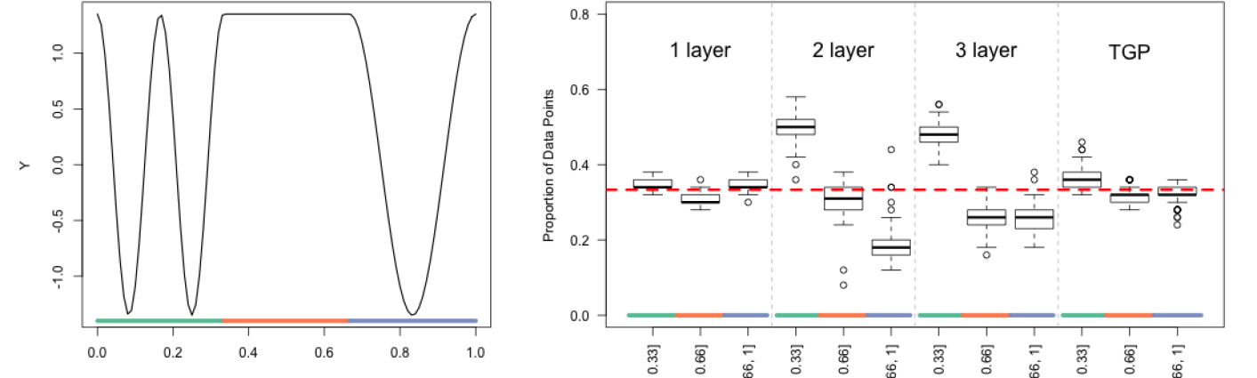
Figure 6: Left: $f(x)$ from Eq. (20). Three regions of the input space are highlighted by the green, orange, and blue lines on the $x$-axis. Right: proportion of sampled points falling in each region. Boxplots represent the spread of 100 repetitions. A red dotted line marks the actual proportion of the input space occupied by each region.

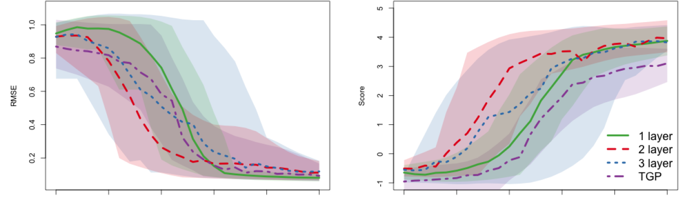
Figure 7: RMSE (left) and score (right) for $f(x)$ from Eq. (20). Solid lines represent the average over 100 repetitions. Shaded regions represent 90% quantiles.

Figure 7 shows RMSE and score calculated after each iteration for the four comparators. The two-layer DGP dramatically outperforms the one-layer GP for small data sizes ($n=10,\dots,25$). Once $n$ is large enough, the one-layer model catches up. This ordinary GP eventually edges out on RMSE, but the two-layer DGP wins on score. The latter’s wider RMSE quantiles at $n=35$ are caused by models that over-fit the noisy observations. The three-layer model performs well on average, but is marked by very wide quantiles due to even more prominent over-fitting. Both DGPs do a better job of placing runs in the region of highest interest, $x\in[0,0.33]$; see Figure 6, right. In the two-layer case, notice the right-hand region $x\in[0.66,1]$ has the fewest acquisitions of all. This happens, we believe, because of the shape of the latent $W$ layer. Refer again to the left panel of Figure 5, where the right-hand region bends toward the left-hand one, “borrowing strength” from the more substantial corpus of information there. Despite a strictly distance-based kernel structure, such latent $W$ may impart a periodic effect on dynamics. The non-stationarity of the TGP model allows some departure from space-filling designs, but performs poorly on score; likely a by-product of model uncertainty in the spatial location of spits outlining partitions of the tree.

2d.

Next consider a 2d example originally from Gramacy and Lee, (2009):

$$f(x_{1},x_{2})=10x_{1}\textrm{exp}\left(-x_{1}^{2}-x_{2}^{2}\right)\quad\textrm{for}\quad x_{1},x_{2}\in[-2,4],$$ (21)

observed with $\mathcal{N}(0,0.1^{2})$ noise. Although there are no abrupt shifts, this function is characterized by two distinct regimes.

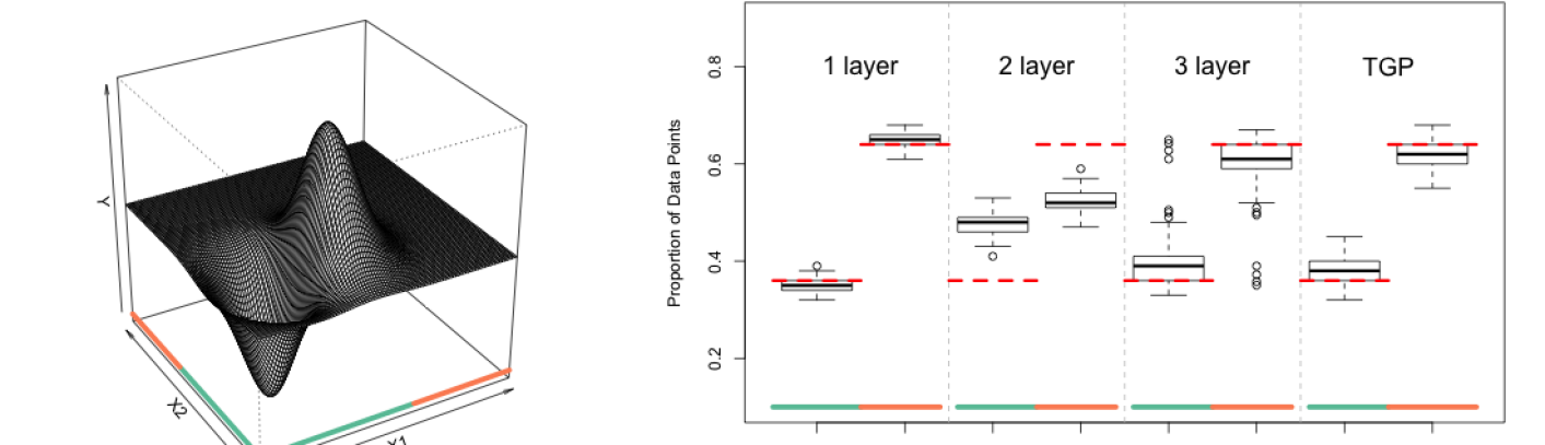
Figure 8: Left: $f(x_{1},x_{2})$ from Eq. (21). Two input regions are marked by the green and orange lines along the $x$-axes. Right: Proportion of AL acquisitions falling in each region. Boxplots indicate spread over 100 repetitions. Red dotted lines mark the actual proportions occupied by each region.

Figure 8 marks these with color along the $x$-axes; naturally the “peaky”, bottom-left region is of more interest than the much larger flat one. AL is initialized with random LHSs of size $n_{0}=10$, followed by ALC acquisitions (200 candidates/references) up to $n=80$.

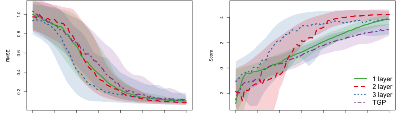
Figure 9: RMSE (left) and score (right) for $f(x_{1},x_{2})$ from Eq. (21). Solid lines represent the average over 100 repetitions. Shaded regions represent 90% quantiles.

Figure 9 shows RMSE and score calculated after each iteration for one-, two-, and three-layer models as well as TGP. The two-layer DGP performs similarly to the one-layer GP in terms of RMSE, but the former achieves consistently higher scores after a modest number of acquisitions ($n>35$). The three-layer DGP beats the others in both metrics on average but has the widest quantiles. As in the 1d case, both deep models do a better job of placing design points in the region of interest; see Figure 8. TGP performs similarly to the one-layer GP.

5.3 Langley Glide-Back Booster

The Langley Glide-Back Booster (LGBB) computer model was designed by NASA to assess the movement of a rocket booster gliding back to Earth for re-use after launching a payload into orbit. A thorough review is provided in Pamadi et al., (2004). The LGBB simulator has three inputs – speed upon entry (mach), angle of attack (alpha), and side-slip angle (beta) – and produces six deterministic response values (lift, drag, pitch, side, yaw, and roll). This model is uniquely non-stationary because the sound barrier at mach 1 imparts regime changes on aeronautic dynamics.

Gramacy and Lee, (2008) developed Bayesian treed Gaussian process (TGP) models specifically to account for these kinds of axis-aligned regime shifts. In our work here, we utilize a dense grid of TGP-surrogate evaluated LGBB response values from one of their AL experiments, in lieu of real simulations (the actual simulator is propriety). Having the “truth” lie inside the TGP-model class elevates this model to gold standard in terms of out-of-sample validation, but nevertheless we find comparison outside that class (with DGPs) to be informative. For more details on these data, and surrogate evaluations, see Gramacy, (2020, Chapter 2).

Here we focus on the side response; dynamics in the other outputs are similar. Figure 10 provides a visual of this response for a fixed beta value. The sound barrier causes a sharp ridge at mach 1. The region with mach values less than 2 is clearly the most “interesting”.

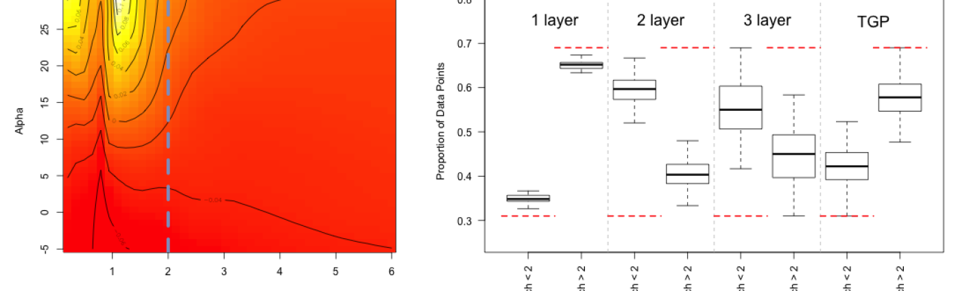
Figure 10: Left: Visual of the LGBB side response for fixed beta = 4. White/high, red/low. A vertical dotted line splits the input region at mach 2. Right: Proportion of 300 sampled points falling left/right of mach 2. Boxplots represent spread over 30 repetitions. Red dotted lines mark actual proportion of input space.

After initializing with a random uniform (sub-) design size $n_{0}=50$ we entertained ALC (500 candidates/references) for acquisitions up to $n=300$ using our usual four comparators. A nugget of $g=10^{-8}$ was fixed to account for the deterministic nature of simulations. RMSE on a 1000-point out-of-sample testing set (newly randomized for each calculation) was evaluated after every 10th acquisition. On those occasions, we re-used the 1000-point testing set as ALC candidates/references. Joint evaluation of predictions and ALC is efficient since both rely on mapped $\mathcal{W}^{(t)}$ (15).

Figure 11 tracks out-of-sample RMSE for the four comparators over AL acquisitions, via averages over thirty MC repetitions (left), and the spread of values after the final AL acquisition (right). Both deep models outperform the one-layer GP model but are unable to match the “gold standard” of TGP. The difference in the allocation of design points among these models is pronounced. See the right panel of Figure 10. The one-layer model is very similar to a space-filling design. TGP deviates from space filling and puts more design points in the region of interest (mach $<2$), but still allocates the majority of points in the flat region. DGPs even more aggressively acquire/learn in the interesting region, placing more than half of the inputs left of mach 2.

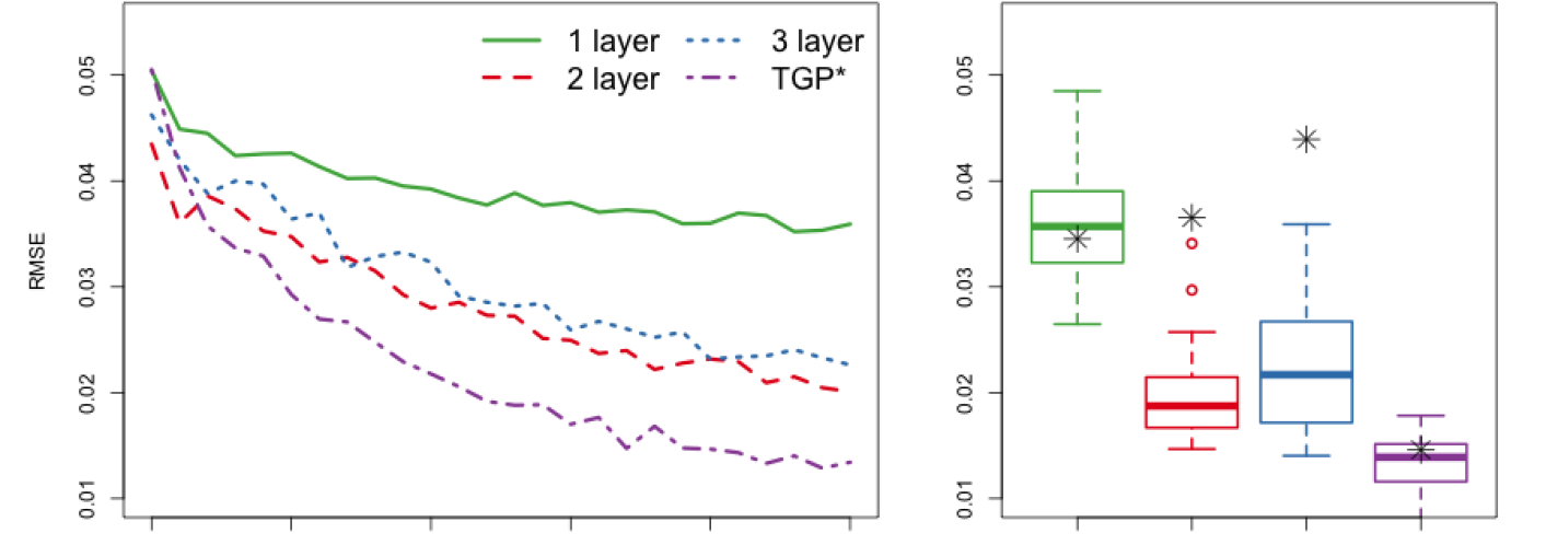
Figure 11: Left: RMSE on out-of-sample 1000 point testing sets for the LGBB computer experiment, averaged over 30 repetitions. Right: spread of final RMSE at $n=300$ across 30 repetitions. Black stars denote the RMSE obtained from static 300-point designs. Both one-layer MLE variants performed equivalently to the one-layer MCMC fit.

To further investigate the benefit of AL with DGPs, we generated a purely random design of size $n=300$ to train each of the four surrogates. These RMSEs are indicated as *s overlayed on the boxplots of their respective AL counterparts in the right panel of Figure 11. Observe that these static design results are substantially worse for the two- and three-layer fits. These DGPs demand non-uniform acquisition to predict well. One-layer results are comparable because these AL designs are essentially space-filling. The TGP results are curious. Apparently, predictive prowess here comes from “serendipitous accuracy”, arising from within-model simulations, more than from AL reinforcement. Finally, we fit a one-layer model using MLE hyperparameters with both separable and non-separable lengthscales using the laGP package (Gramacy,, 2016). These RMSEs are identical to those obtained from the one-layer fit, with stars obscuring one another in the figure. We took this as in indication that the experiment was internally well-calibrated.

5.4 Satellite drag

Researchers at Los Alamos National Laboratory developed the Test Particle Monte Carlo simulator to compute drag coefficients for satellites in low earth orbit. These are useful in the development of positioning and collision avoidance systems. Sun et al., (2019) created an R wrapper for the simulator and made it publicly available (https://bitbucket.org/gramacylab/tpm/). The simulator relies on a geometric satellite specification, atmospheric composition, and 7 input variables. See Sun et al., (2019) and Gramacy, (2020, Chapter 2) for a thorough discussion of the simulator and its inputs. We consider the GRACE satellite here; details on atmospheric composition settings are available in our public Git repository. Each simulation takes about 86 seconds on a modern desktop.

Mehta et al., (2014) showed that over a restricted portion of the input space, a GP surrogate trained via 1000-point LHS is able to predict drag within 1% root mean square percentage error (RMSPE). We use Mehta’s work as a benchmark and show that sequentially designed DGP models can achieve predictions within 1% RMSPE with fewer data points. We begin with a 7d LHS of size $n_{0}=100$. To help our model properly estimate the noise of the stochastic simulator we ran (multiplicity two) replicates at a random selection of ten of these original locations, so our training actually comprised of $n_{0}=110$ runs. To measure out-of-sample accuracy by RMSPE, and thus benchmark against Mehta et al.,, we built a single 1000-element testing set via LHS.

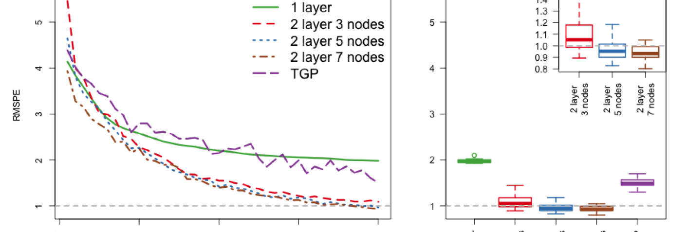
Figure 12: Left: out-of-sample average RMSPE for sequential design of the satellite drag simulator over ten repetitions. Right: spread of final RMSPE at $n=500$ across 10 repetitions. Dashed lines highlight the 1% goal. The top-right sub-panel zooms in on the best comparators.

Considering the substantial simulator expense, we did not entertain three-layer DGPs. Our previous experiments suggested that three-layer models were overkill, and potentially risky. Although their average-case behavior was attractive, it was also more volatile over repetitions. However, considering the larger input dimension compared to those earlier exercises, we did variations in latent dimension, with $p\in\{3,5,7\}$. In all three cases, training data inputs were sequentially selected using ALC (1000 candiates/references) up to $n=500$, and RMSPE on the testing set was evaluated after every 10th acquisition. Again due to simulator expense, we limited the MC exercise to ten repetitions (only five for TGP). Results are summarized in Figure 12.

Observe that all but the one-layer (ordinary GP) and TGP comparators were able to achieve the 1% benchmark, with high probability, with fewer than 500 runs of the simulator. Interestingly, it is possible to accomplish this feat with a latent dimension of $p=3\ll d=7$. Although results are improved with more latent dimensions, up to $p=d=7$ which is the software default, this comes at greater computational expense ($p=3$ is two times faster on an eight core machine).

6 Conclusion

We provided a novel Gibbs-ESS-Metropolis method for fitting deep Gaussian processes (DGPs), specifically targeted to surrogate modeling applications. Their nonstationary nature makes them an excellent candidate for sequential design via active learning (AL) when simulation dynamics are characterized by stark regime shifts. In addition to illustrations of component parts of our inferential and AL scheme(s), we demonstrated how DGP models outperformed typical GP regression in examples ranging up to seven dimensions.

Several modeling choices were made in order to protect identifiability and to favor simplicity. These were motivated by challenges brought to light in empirical work behind earlier incantations. Examples include enforcing common dimensionality in latent layers, limiting depth to three-layers (or even two), and limiting nodes to no more than the input dimension. These constraints seem to provide a degree of regularization which does not overly hinder reactivity of the apparatus, and appears to be essential in AL settings. Early on, when the training design is small, strong regularization helps encourage stability. In later stages, after many runs have been acquired, the information in the likelihood is able to dominate the prior. We submit our favorable empirical outcomes, on a relatively broad range of synthetic and real-simulator AL examples, as evidence. However, a more detailed cost-benefit analysis of DGP complexity v. prowess may be warranted.

We were most surprised by how well a simple default setup – two layers with nodes matching the input dimension $(p=d)$ – compared to more complex alternatives. Although there is evidence that even deeper GPs ($\geq 3$ latent layers) work well when there are abrupt regime shifts (Damianou and Lawrence,, 2013; Dunlop et al.,, 2018), we were unable to identify any common computer simulation benchmarks which demanded that complexity. It may be that typical simulators simply aren’t that pathological. Perhaps incorporating input connected networks (Duvenaud et al.,, 2014), in which deep layers depend on both the previous layer and the original inputs, may increase the utility of deeper models. In higher dimensional settings, we found the relative success of two-layer DGPs with $p<d$ to be intriguing. Our work was limited to post-hoc analysis of depth and node size; selecting these specifications in real-time, for example, would be of great practical interest.

The recent success of DGPs as surrogates, such as for calibration (Marmin and Filippone,, 2018), multi-fidelity modeling (Cutajar et al.,, 2019), and black-box optimization (Hebbal et al.,, 2021), is exciting. UQ plays a key role in each of these, yet approximation via maximization is the modus operandi. Consequently, such surrogates under-estimate – or at best mis-characterize – relevant uncertainties. Our novel Gibbs-ESS-Metropolis scheme may make MCMC tractable where it wasn’t previously effective, and the additional UQ may result in significant improvements.

The additional computation required to fit DGP models poses a challenge for larger sample sizes. Our MCMC method is not appropriate when data is abundant. Potential remedies include incorporating inducing points (Rajaram et al.,, 2021) and/or utilizing the covariance function or operator formulations of Dunlop et al., (2018). Moreover, it may be possible to implement sequential model updates in our framework following Wang et al., (2016).

Acknowledgements

This work was supported by the U.S. Department of Energy, Office of Science, Office of Advanced Scientific Computing Research and Office of High Energy Physics, Scientific Discovery through Advanced Computing (SciDAC) program under Award Number 0000231018. We also thank referees for their valuable insights and suggestions that led to an improved manuscript.

SUPPLEMENTARY MATERIAL

Illustration of ALC surface for the 2d example and derivations of IMSE (18) and ALC (19).

SUPPLEMENTARY MATERIAL

Appendix A ALC Illustration

A.1 2d ALC Surface

For another illustration, consider a typical, stationary GP surrogate fit to simulations following Eq. (21), detailed in Section 5.2. The left panel of Figure 13 shows ALC, using a dense $X_{\mathrm{ref}}$ grid, after training on evaluations obtained from an LHS of size $n=30$. In this example, the lower left corner is the area of highest interest, but ALC is, in essence, a function of proximity to $X_{n}$. A two-layer DGP fit to the same training data is able to allocate uncertainty in the “interesting” region, resulting in non-space filling acquisitions.

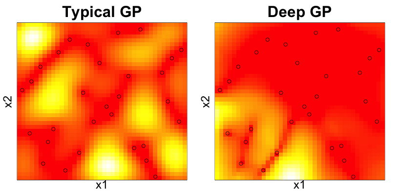
Figure 13: Heat map of ALC surface for typical GP and two-layer DGP surrogates (via MCMC) for $f(x_{1},x_{2})$ in Eq. (21). Open circles indicate design $X_{n}$. White/high, red/low.

Appendix B Derivations

B.1 Partitioned Matrix Inverse

Following the properties of partitioned matrices (e.g., Barnett,, 1979), with $k_{n}(w_{n+1})=K_{\theta_{y}}(W_{n},w_{n+1})$,

$$C_{n+1}=\begin{bmatrix}C_{n}&k_{n}(w_{n+1})\\ k_{n}^{\top}(w_{n+1})&1+g\end{bmatrix}\quad\mathrm{yields}\quad C_{n+1}^{-1}=\begin{bmatrix}\left[C_{n}^{-1}+hh^{\top}v\right]&h\\ h^{\top}&v^{-1}\end{bmatrix}$$

where $v=1+g-k_{n}^{\top}(w_{n+1})C_{n}^{-1}k_{n}(w_{n+1})$ and $h=-v^{-1}C_{n}^{-1}k_{n}(w_{n+1})$.

B.2 IMSE Derivation

Here we extend the closed-form IMSE derivation of Binois et al., (2019) to allow integration under uniform measure over the general domain $W_{i}\in[a_{i},b_{i}]$ for $i=1,\dots,p$ for the model $Y\sim N_{n}(0,K_{\theta_{y}}(W)+g\mathbb{I})$ and isotropic Gaussian kernel (1). Application to MCMC samples requires indexing with iteration $(t)$, but we drop this notation here for convenience. We set $\Sigma(w)=1$ instead of $\Sigma(w)=1+g$ to target the variance of the mean.

Using $W_{n+1}$ and $C_{n+1}$ as described in Section 4.2, and additionally denoting $k_{n+1}(w)=K_{\theta_{y}}(W_{n+1},w)$, IMSE may be expressed as follows.

$$\textrm{IMSE}(W_{n+1}) =\int_{a_{p}}^{b_{p}}\dots\int_{a_{1}}^{b_{1}}\Sigma_{Y}(w)\;dw_{1}\dots dw_{p}$$

$$=\prod_{i=1}^{p}(b_{i}-a_{i})\mathbb{E}\left[\Sigma_{Y}(w)\right]$$

$$=\prod_{i=1}^{p}(b_{i}-a_{i})\mathbb{E}\left[\hat{\tau}^{2}\left(1-k^{\top}_{n+1}(w)C_{n+1}^{-1}k_{n+1}(w)\right)\right]$$

$$=\hat{\tau}^{2}\prod_{i=1}^{p}(b_{i}-a_{i})\left[1-\mathbb{E}\left[k^{\top}_{n+1}(w)C_{n+1}^{-1}k_{n+1}(w)\right]\right]$$

This expectation reduces to a trace of matrix products following Lemma 3.1 of Binois et al., (2019),

$$\mathbb{E}\left[k^{\top}_{n+1}(w)C_{n+1}^{-1}k_{n+1}(w)\right]=\mathrm{tr}\left(C_{n+1}^{-1}H\right),$$

where the elements of $H$ are defined as

$$H_{jk} =\prod_{i=1}^{p}\int_{a_{i}}^{b_{i}}K_{\theta_{y}}(w_{j,i},w)K_{\theta_{y}}(w_{k,i},w)\;dw_{i}$$

$$=\prod_{i=1}^{p}\int_{a_{i}}^{b_{i}}\mathrm{exp}\left(\frac{-(w_{j,i}-w)^{2}}{\theta_{y}}\right)\mathrm{exp}\left(\frac{-(w_{k,i}-w)^{2}}{\theta_{y}}\right)\;dw_{i}$$

$$=\prod_{i=1}^{p}\int_{a_{i}}^{b_{i}}\mathrm{exp}\left(-\frac{2}{\theta_{y}}\left(w-\frac{w_{j,i}+w_{k,i}}{2}\right)^{2}-\frac{1}{2\theta_{y}}(w_{j,i}-w_{k,i})^{2}\right)\;dw_{i}$$

$$=\prod_{i=1}^{p}\left[\mathrm{exp}\left(-\frac{(w_{j,i}-w_{k,i})^{2}}{2\theta_{y}}\right)\int_{a_{i}}^{b_{i}}\mathrm{exp}\left(-\frac{2}{\theta_{y}}\left(w-\frac{w_{j,i}+w_{k,i}}{2}\right)^{2}\right)\;dw_{i}\right]$$

$$=\prod_{i=1}^{p}\left[\sqrt{\frac{\pi\theta_{y}}{2}}\mathrm{exp}\left(-\frac{(w_{j,i}-w_{k,i})^{2}}{2\theta_{y}}\right)\int_{a_{i}}^{b_{i}}\mathcal{N}\left(w\mid\mu=\frac{w_{j,i}+w_{k,i}}{2},\sigma^{2}=\frac{\theta_{y}}{4}\right)\;dw_{i}\right]$$

$$=\left(\frac{\pi\theta_{y}}{2}\right)^{\frac{p}{2}}\prod_{i=1}^{p}\left\{\mathrm{exp}\left(-\frac{(w_{j,i}-w_{k,i})^{2}}{2\theta_{y}}\right)\left[\Phi\left(\frac{2b_{i}-w_{j,i}-w_{k,i}}{\sqrt{\theta_{y}}}\right)-\Phi\left(\frac{2a_{i}-w_{j,i}-w_{k,i}}{\sqrt{\theta_{y}}}\right)\right]\right\}.$$

Above, $w_{j,i}$ is the $j^{th}$ element of the $i^{th}$ node of $W$ and $\Phi$ is the standard Gaussian cumulative distribution function (CDF).

B.3 ALC Derivation

Here, we detail the re-expression of ALC from Eq. (19) in terms of the new latent element, $w_{n+1}$. Again, we drop $(t)$ indexing to streamline. Quantities $k_{n}(w)$, $v$, and $h$ are defined in Appendix B.1 and yield partitioned representation of $k_{n+1}^{\top}(w)=\begin{bmatrix}k_{n}^{\top}(w)\mid z\end{bmatrix}$ where $z=K_{\theta_{y}}(w_{n+1},w)$. Tedious matrix multiplication gives

$$k_{n+1}^{\top}(w)C_{n+1}^{-1}k_{n+1}(w) =\begin{bmatrix}k_{n}^{\top}(w)\mid z\end{bmatrix}\begin{bmatrix}C_{n}^{-1}+hh^{\top}v&h\\ h^{\top}&v^{-1}\end{bmatrix}\begin{bmatrix}k_{n}(w)\\ z\end{bmatrix}$$

$$=\begin{bmatrix}k_{n}^{\top}(w)\left(C_{n}^{-1}+hh^{\top}v\right)+zh^{\top}\mid k_{n}^{\top}(w)h+zv^{-1}\end{bmatrix}\begin{bmatrix}k_{n}(w)\\ z\end{bmatrix}$$

$$=k_{n}^{\top}(w)(C_{n}^{-1}+hh^{\top}v)k_{n}(w)+zh^{\top}k_{n}(w)+k_{n}^{\top}(w)hz+v^{-1}z^{2}$$

$$=k_{n}^{\top}(w)C_{n}^{-1}k_{n}(w)+v(k_{n}^{\top}(w)h)^{2}+2zk_{n}^{\top}(w)h+v^{-1}z^{2}$$

$$\propto v(k_{n}^{\top}(w)h)^{2}+2zk_{n}^{\top}(w)h+v^{-1}z^{2},$$

producing the following ALC

$$\mathrm{ALC}(w_{n+1}\mid\mathcal{W}_{\mathrm{ref}})\propto\sum_{w\in\mathcal{W}_{\mathrm{ref}}}\hat{\tau}^{2}\left[v(h^{\top}k_{n}(w))^{2}+2zh^{\top}k_{n}(w)+v^{-1}z^{2}\right].$$

References

- Ba and Joseph, (2012) Ba, S. and Joseph, V. R. (2012). “Composite Gaussian process models for emulating expensive functions.” The Annals of Applied Statistics, 1838–1860.
- Barnett, (1979) Barnett, S. (1979). Matrix methods for engineers and scientists. McGraw-Hill.
- Berger et al., (2001) Berger, J. O., De Oliveira, V., and Sansó, B. (2001). “Objective Bayesian analysis of spatially correlated data.” Journal of the American Statistical Association, 96, 456, 1361–1374.
- Binois et al., (2019) Binois, M., Huang, J., Gramacy, R. B., and Ludkovski, M. (2019). “Replication or Exploration? Sequential Design for Stochastic Simulation Experiments.” Technometrics, 61, 1, 7–23.
- Bornn et al., (2012) Bornn, L., Shaddick, G., and Zidek, J. V. (2012). “Modeling nonstationary processes through dimension expansion.” Journal of the American Statistical Association, 107, 497, 281–289.
- Bui et al., (2016) Bui, T., Hernández-Lobato, D., Hernandez-Lobato, J., Li, Y., and Turner, R. (2016). “Deep Gaussian processes for regression using approximate expectation propagation.” In International conference on machine learning, 1472–1481. PMLR.
- Cohn, (1994) Cohn, D. (1994). “Neural network exploration using optimal experiment design.” In Advances in Neural Information Processing Systems, vol. 6, 679–686. Morgan-Kaurmann.
- Cole et al., (2021) Cole, D. A., Christianson, R. B., and Gramacy, R. B. (2021). “Locally induced Gaussian processes for large-scale simulation experiments.” Statistics and Computing, 31, 3, 1–21.
- Cutajar et al., (2019) Cutajar, K., Pullin, M., Damianou, A., Lawrence, N., and González, J. (2019). “Deep gaussian processes for multi-fidelity modeling.” arXiv preprint arXiv:1903.07320.
- Damianou and Lawrence, (2013) Damianou, A. and Lawrence, N. D. (2013). “Deep gaussian processes.” In Artificial intelligence and statistics, 207–215. PMLR.
- Deissenberg et al., (2009) Deissenberg, C., Van Der Hoog, S., and Dawid, H. (2009). “EURACE: A massively parallel agent-based model of the European economy.” Applied Mathematics and Computation, 204, 2, 541–552.
- Dunlop et al., (2018) Dunlop, M. M., Girolami, M. A., Stuart, A. M., and Teckentrup, A. L. (2018). “How deep are deep Gaussian processes?” Journal of Machine Learning Research, 19, 54, 1–46.
- Dutordoir et al., (2017) Dutordoir, V., Knudde, N., van der Herten, J., Couckuyt, I., and Dhaene, T. (2017). “Deep Gaussian process metamodeling of sequentially sampled non-stationary response surfaces.” In 2017 Winter Simulation Conference (WSC), 1728–1739. IEEE.
- Duvenaud et al., (2014) Duvenaud, D., Rippel, O., Adams, R., and Ghahramani, Z. (2014). “Avoiding pathologies in very deep networks.” In Artificial Intelligence and Statistics, 202–210. PMLR.
- Fadikar et al., (2018) Fadikar, A., Higdon, D., Chen, J., Lewis, B., Venkatramanan, S., and Marathe, M. (2018). “Calibrating a stochastic, agent-based model using quantile-based emulation.” SIAM/ASA Journal on Uncertainty Quantification, 6, 4, 1685–1706.
- Fei et al., (2018) Fei, J., Zhao, J., Sun, S., and Liu, Y. (2018). “Active Learning Methods with Deep Gaussian Processes.” In International Conference on Neural Information Processing, 473–483. Springer.
- Gelman et al., (2013) Gelman, A., Carlin, J. B., Stern, H. S., Dunson, D. B., Vehtari, A., and Rubin, D. B. (2013). Bayesian data analysis. CRC press.
- Gneiting and Raftery, (2007) Gneiting, T. and Raftery, A. E. (2007). “Strictly proper scoring rules, prediction, and estimation.” Journal of the American statistical Association, 102, 477, 359–378.
- Gramacy, (2007) Gramacy, R. B. (2007). “tgp: An R Package for Bayesian Nonstationary, Semiparametric Nonlinear Regression and Design by Treed Gaussian Process Models.” Journal of Statistical Software, 19, 9, 1–46.
- Gramacy, (2016) — (2016). “laGP: Large-Scale Spatial Modeling via Local Approximate Gaussian Processes in R.” Journal of Statistical Software, 72, 1, 1–46.
- Gramacy, (2020) — (2020). Surrogates: Gaussian Process Modeling, Design and Optimization for the Applied Sciences. Boca Raton, Florida: Chapman Hall/CRC. http://bobby.gramacy.com/surrogates/.
- Gramacy and Apley, (2015) Gramacy, R. B. and Apley, D. W. (2015). “Local Gaussian process approximation for large computer experiments.” Journal of Computational and Graphical Statistics, 24, 2, 561–578.
- Gramacy and Lee, (2008) Gramacy, R. B. and Lee, H. K. H. (2008). “Bayesian treed Gaussian process models with an application to computer modeling.” Journal of the American Statistical Association, 103, 483, 1119–1130.
- Gramacy and Lee, (2009) — (2009). “Adaptive Design and Analysis of Supercomputer Experiments.” Technometrics, 51, 2, 130–145.
- Havasi et al., (2018) Havasi, M., Hernández-Lobato, J. M., and Murillo-Fuentes, J. J. (2018). “Inference in deep gaussian processes using stochastic gradient hamiltonian monte carlo.” In Advances in neural information processing systems, 7506–7516.
- Hebbal et al., (2021) Hebbal, A., Brevault, L., Balesdent, M., Talbi, E.-G., and Melab, N. (2021). “Bayesian optimization using deep Gaussian processes with applications to aerospace system design.” Optimization and Engineering, 22, 1, 321–361.
- Higdon et al., (2004) Higdon, D., Kennedy, M., Cavendish, J. C., Cafeo, J. A., and Ryne, R. D. (2004). “Combining field data and computer simulations for calibration and prediction.” SIAM Journal on Scientific Computing, 26, 2, 448–466.
- Higdon et al., (1999) Higdon, D., Swall, J., and Kern, J. (1999). “Non-stationary spatial modeling.” Bayesian statistics, 6, 1, 761–768.
- Higdon et al., (2003) Higdon, D. M., Lee, H., and Holloman, C. (2003). “Markov chain Monte Carlo-based approaches for inference in computationally intensive inverse problems (with discussion).” In Bayesian Statistics 7. Proceedings of the Seventh Valencia International Meeting, eds. J. M. Bernardo, M. J. Bayarri, J. O. Berger, A. P. Dawid, D. Heckerman, A. F. M. Smith, and M. West, 181–197. Oxford University Press.
- Johnson et al., (1990) Johnson, M. E., Moore, L. M., and Ylvisaker, D. (1990). “Minimax and maximin distance designs.” Journal of statistical planning and inference, 26, 2, 131–148.
- Jones et al., (1998) Jones, D. R., Schonlau, M., and Welch, W. J. (1998). “Efficient global optimization of expensive black-box functions.” Journal of Global optimization, 13, 4, 455–492.
- Kass et al., (1998) Kass, R. E., Carlin, B. P., Gelman, A., and Neal, R. M. (1998). “Markov chain Monte Carlo in practice: a roundtable discussion.” The American Statistician, 52, 2, 93–100.
- Katzfuss, (2013) Katzfuss, M. (2013). “Bayesian nonstationary spatial modeling for very large datasets.” Environmetrics, 24, 3, 189–200.
- Kennedy and O’Hagan, (2001) Kennedy, M. C. and O’Hagan, A. (2001). “Bayesian calibration of computer models.” Journal of the Royal Statistical Society: Series B (Statistical Methodology), 63, 3, 425–464.
- MacKay, (1992) MacKay, D. J. (1992). “Information-based objective functions for active data selection.” Neural computation, 4, 4, 590–604.
- Marmin and Filippone, (2018) Marmin, S. and Filippone, M. (2018). “Variational calibration of computer models.” arXiv preprint arXiv:1810.12177.
- Marrel et al., (2009) Marrel, A., Iooss, B., Laurent, B., and Roustant, O. (2009). “Calculations of sobol indices for the gaussian process metamodel.” Reliability Engineering & System Safety, 94, 3, 742–751.
- McKay et al., (2000) McKay, M. D., Beckman, R. J., and Conover, W. J. (2000). “A comparison of three methods for selecting values of input variables in the analysis of output from a computer code.” Technometrics, 42, 1, 55–61.
- Mehta et al., (2014) Mehta, P. M., Walker, A., Lawrence, E., Linares, R., Higdon, D., and Koller, J. (2014). “Modeling satellite drag coefficients with response surfaces.” Advances in Space Research, 54, 8, 1590–1607.
- Microsoft and Weston, (2020) Microsoft and Weston, S. (2020). foreach: Provides Foreach Looping Construct. R package version 1.5.0.
- Morris and Mitchell, (1995) Morris, M. D. and Mitchell, T. J. (1995). “Exploratory designs for computational experiments.” Journal of statistical planning and inference, 43, 3, 381–402.
- Murray et al., (2010) Murray, I., Adams, R. P., and MacKay, D. J. C. (2010). “Elliptical slice sampling.” In The Proceedings of the 13th International Conference on Artificial Intelligence and Statistics, vol. 9 of JMLR: W&CP, 541–548. PMLR.
- Neal, (2011) Neal, R. M. (2011). “MCMC using Hamiltonian dynamics.” Handbook of Markov chain Monte Carlo, 2, 11, 2.
- Oakley and O’Hagan, (2004) Oakley, J. E. and O’Hagan, A. (2004). “Probabilistic sensitivity analysis of complex models: a Bayesian approach.” Journal of the Royal Statistical Society: Series B (Statistical Methodology), 66, 3, 751–769.
- Oliver et al., (1997) Oliver, D. S., Cunha, L. B., and Reynolds, A. C. (1997). “Markov chain Monte Carlo methods for conditioning a permeability field to pressure data.” Mathematical Geology, 29, 1, 61–91.
- Paciorek and Schervish, (2003) Paciorek, C. J. and Schervish, M. J. (2003). “Nonstationary Covariance Functions for Gaussian Process Regression.” In Proceedings of the 16th International Conference on Neural Information Processing Systems, NIPS’03, 273–280. Cambridge, MA, USA: MIT Press.
- Pamadi et al., (2004) Pamadi, B., Covell, P., Tartabini, P., and Murphy, K. (2004). “Aerodynamic characteristics and glide-back performance of langley glide-back booster.” In 22nd Applied Aerodynamics Conference and Exhibit, 5382.
- Picheny et al., (2016) Picheny, V., Gramacy, R., Wild, S., and Le Digabel, S. (2016). “Bayesian optimization under mixed constraints with a slack-variable augmented Lagrangian.” In Advances in Neural Information Processing Systems, 1435–1443.
- Radaideh and Kozlowski, (2020) Radaideh, M. I. and Kozlowski, T. (2020). “Surrogate modeling of advanced computer simulations using deep Gaussian processes.” Reliability Engineering & System Safety, 195, 106731.
- Rajaram et al., (2021) Rajaram, D., Puranik, T. G., Ashwin Renganathan, S., Sung, W., Fischer, O. P., Mavris, D. N., and Ramamurthy, A. (2021). “Empirical assessment of deep gaussian process surrogate models for engineering problems.” Journal of Aircraft, 58, 1, 182–196.
- Rasmussen, (2000) Rasmussen, C. E. (2000). “The Infinite Gaussian Mixture Model.” In In Advances in Neural Information Processing Systems 12, 554–560. MIT Press.
- Rasmussen and Ghahramani, (2002) Rasmussen, C. E. and Ghahramani, Z. (2002). “Infinite mixtures of Gaussian process experts.” In Advances in neural information processing systems, vol. 2, 881–888. MIT.
- Rasmussen and Williams, (2005) Rasmussen, C. E. and Williams, C. K. I. (2005). Gaussian Processes for Machine Learning. Cambridge, Mass.: MIT Press.
- Salimbeni and Deisenroth, (2017) Salimbeni, H. and Deisenroth, M. (2017). “Doubly stochastic variational inference for deep Gaussian processes.” arXiv preprint arXiv:1705.08933.
- Saltelli, (2002) Saltelli, A. (2002). “Making best use of model evaluations to compute sensitivity indices.” Computer physics communications, 145, 2, 280–297.
- Sampson and Guttorp, (1992) Sampson, P. D. and Guttorp, P. (1992). “Nonparametric estimation of nonstationary spatial covariance structure.” Journal of the American Statistical Association, 87, 417, 108–119.
- Santner et al., (2018) Santner, T., Williams, B., and Notz, W. (2018). The Design and Analysis of Computer Experiments, Second Edition. New York, NY: Springer–Verlag.
- Sauer, (2020) Sauer, A. (2020). deepgp: Sequential Design for Deep Gaussian Processes using MCMC. R package version 0.1.0.
- Schmidt and O’Hagan, (2003) Schmidt, A. M. and O’Hagan, A. (2003). “Bayesian inference for non-stationary spatial covariance structure via spatial deformations.” Journal of the Royal Statistical Society: Series B (Statistical Methodology), 65, 3, 743–758.
- Sejdinovic et al., (2014) Sejdinovic, D., Strathmann, H., Garcia, M. L., Andrieu, C., and Gretton, A. (2014). “Kernel adaptive metropolis-hastings.” In International conference on machine learning, 1665–1673. PMLR.
- Seo et al., (2000) Seo, S., Wallat, M., Graepel, T., and Obermayer, K. (2000). “Gaussian process regression: active data selection and test point rejection.” In Proceedings of the IEEE-INNS-ENNS International Joint Conference on Neural Networks, vol. 3, 241–246. IEEE.
- Shewry and Wynn, (1987) Shewry, M. C. and Wynn, H. P. (1987). “Maximum entropy sampling.” Journal of applied statistics, 14, 2, 165–170.
- Snoek et al., (2012) Snoek, J., Larochelle, H., and Adams, R. P. (2012). “Practical Bayesian optimization of machine learning algorithms.” In Advances in Neural Information Processing Systems, vol. 25, 2951–2959. Curran Associates Inc.
- Stein, (1999) Stein, M. L. (1999). Interpolation of spatial data. Springer-Verlag.
- Sun et al., (2019) Sun, F., Gramacy, R. B., Haaland, B., Lawrence, E., and Walker, A. (2019). “Emulating satellite drag from large simulation experiments.” SIAM/ASA Journal on Uncertainty Quantification, 7, 2, 720–759.
- Wang et al., (2016) Wang, Y., Brubaker, M., Chaib-Draa, B., and Urtasun, R. (2016). “Sequential inference for deep Gaussian process.” In Artificial Intelligence and Statistics, 694–703. PMLR.
- Yang and Klabjan, (2020) Yang, J. and Klabjan, D. (2020). “Bayesian Active Learning for Choice Models With Deep Gaussian Processes.” IEEE Transactions on Intelligent Transportation Systems, 22, 2, 1080–1092.
- Zhang et al., (2021) Zhang, B., Cole, D. A., and Gramacy, R. B. (2021). “Distance-distributed design for Gaussian process surrogates.” Technometrics, 63, 1, 40–52.