NeurIPS 2020 Competition:
Predicting Generalization in Deep Learning (Version 1.1)

Abstract

Understanding generalization in deep learning is arguably one of the most important questions in deep learning. Deep learning has been successfully adopted to a large number of problems ranging from pattern recognition to complex decision making, but many recent researchers have raised many concerns about deep learning, among which the most important is generalization. Despite numerous attempts, conventional statistical learning approaches have yet been able to provide a satisfactory explanation on why deep learning works. A recent line of works aims to address the problem by trying to predict the generalization performance through complexity measures. In this competition, we invite the community to propose complexity measures that can accurately predict generalization of models. A robust and general complexity measure would potentially lead to a better understanding of deep learning’s underlying mechanism and behavior of deep models on unseen data, or shed light on better generalization bounds. All these outcomes will be important for making deep learning more robust and reliable.

Keywords

Generalization, Deep Learning, Complexity Measures

Competition type

Regular.

1 Competition description

1.1 Background and impact

Deep learning has been successful in a wide variety of tasks, but a clear understanding of underlying root causes that control generalization of neural networks is still elusive. A recent empirical study [14] looked into many popular complexity measures. By a carefully controlled analysis on hyperparameter choices being a confounder for both generalization and the complexity measure, they came to surprising findings about which complexity measures worked well and which did not. However, rigorously evaluating these complexity measures required training many neural networks, computing the complexity measures on them, and analyzing statistics that condition over all variations in hyperparameters. Such cumbersome process makes it painstaking, error-prone, and computationally expensive. As the results, this procedure is not accessible to members of the wider machine learning community who do not have access to larger compute power.

By hosting this competition, we intend to provide a platform where participants only need to write the code that computes the complexity measure for a trained neural network, and let the competition evaluation framework handle the rest. This way, participants can focus their efforts on coming up with the best complexity measure instead of replicating the experimental set up. In addition, the ML community benefits from results that are directly comparable with each other, which alleviates the need for having every researcher to reproduce all the benchmark results themselves.

This problem is likely to be of interest to machine learning researchers who study generalization of deep learning or experts in learning theory, and the neural architecture search community. We hope that this competition would enable researchers to quickly test theories of generalization with a shorter feedback loop, thereby leading to stronger foundations for designing high-performance, efficient, and reliable deep learning algorithms/architectures. In addition, the fact that all proposed approaches are assessed within the same evaluation system can ensure a fair and transparent evaluation procedure.

This competition is unlike a typical supervised-learning competition – participants are not given a large and representative training set for training a model to produce predictions on an unlabelled test set. Instead, participants submit code, which would run on our evaluation server, and the results would be published on a public leaderboard updated on a daily basis. They are given a small set of models for debugging their code, but this set is not expected to be sufficient for training their model. Their code is expected to take a training dataset of image label pairs as well as a model fully trained on it as input, and generate a real number as output. The value of the output should ideally be larger for models that have larger generalization gaps.

Generalization is one the most fundamental question of machine learning. A principled understanding of generalization can provide theoretical guarantees for machine learning algorithms, which makes deep learning more accountable and transparent, and is also desirable in safety critical applications. For example, generalization to different environments and data distribution shifts is a critical aspect for deploying autonomous vehicles in real life. The result of this competition could also have implications for more efficient architecture search which could reduce the carbon footprint of designing machine learning models and have environmental impact in the long run.

1.2 Novelty

This competition is quite unique, and there are no previous competitions similar to it. The competition is focused on achieving better theory and understanding of the observed phenomena. We hope the competition will allow the fair comparison of numerous theories the community has proposed about generalization of deep learning; however, we also welcome the broader data science community to find practical solutions that are robust under the covariate shift in data and architecture, but do not necessarily give rise statistical bounds or direct theoretical analysis.

1.3 Data

As previously outlined, our competition differs from the traditional supervised learning setting, because our data-points are trained neural networks. As such, the dataset provided to competitors will be a collection of trained neural networks. We chose the Keras API (integrated with TensorFlow 2.x) for its ease of use and the familiarity that a large part of the community has developed with it. Furthermore, all our models will be sequential (i.e., no skip-connections), making it more intuitive for the competitors to explore the architecture of each network. To remove a potential confounding factor, all models are trained until they reach the interpolation regime (close to 100% accuracy on the training set or to a fixed cross entropy value). Each model is represented by a JSON file describing its architecture and a set of trained weights (HDF5 format). We provide the helper functions needed to load a model from those files.

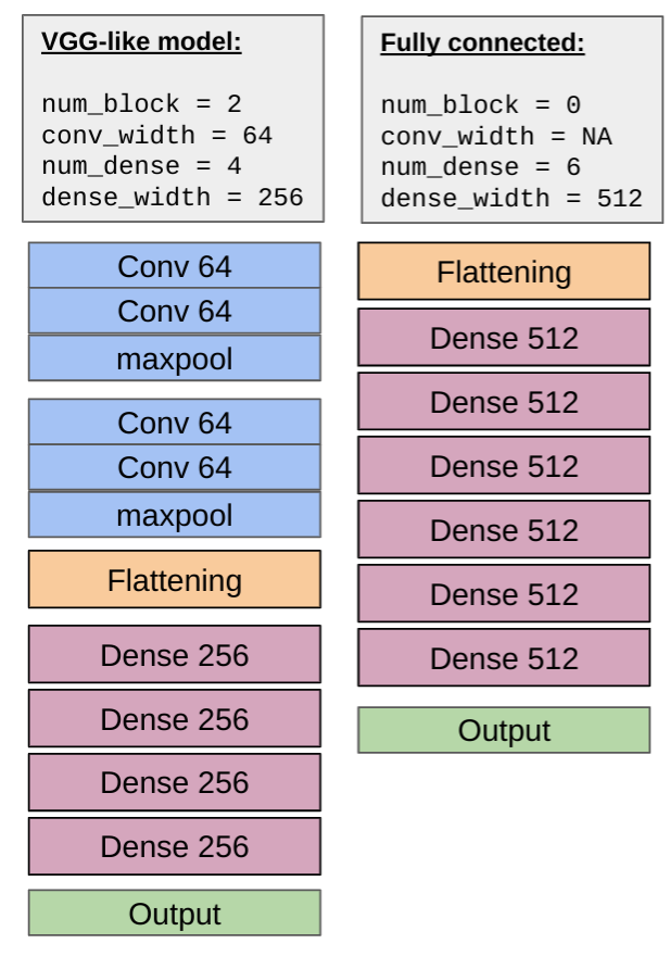
(a) Architecture followed by VGG-like models.

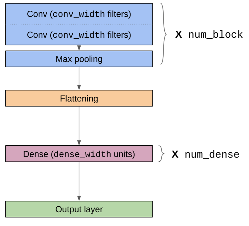
(b) Architectures for two sets of VGG-like hyper parameters.

Figure 1: Example architectures of the networks in our dataset.

The first architecture type we consider is derived from the parameterized architecture described in Figure 1(a). Due to its similarity to the VGG model [30], we will refer to it as VGG-like models. The second connectivity pattern we consider resembles [16] (referred later as Network in network which is generally more parameter efficient than VGG models due to the usage of global average pooling yet yields competitive performance.

• These types of models are well represented in the literature. Inspired by the seminal work of [30], they made their way into an important body of theoretical research in deep learning, see for instance [8, 17, 12]; however, the exact nature of their generalization is still not well understood.

• Empirically, these models reach the interpolating regime quite easily for a large number of optimizers / regularization, while exhibiting a large range of out of sample accuracy (sometime up to 20% of test accuracy difference, for two model with the same architecture and regularization, both reaching 100% training accuracy, depending on the optimizer / learning rate / batch size). In other words, we select these architectures as they often exhibit large generalization gaps and are thus well-suited for this competition.

• These architectures keep the number of hyper-parameters reasonable while exploring a large range of neural network types (fully connected or convolutional, deep or shallow, with convolutional / dense bottlenecks or not), although future iterations of the competition may include arbitrary type of computational graph.

It is worth noting that the optimization method chosen will not be visible to the competitor (i.e. dropout layers will be removed and optimizer is not an attribute of the model), although certain aspects of the hyperparameters can be inferred from the models (e.g. depth or width).

1.3.1 Public and private tasks

The competition is composed of the the following phases:

• Phase 0: Public data was given to the competitors: they were able to download Task 1 and Task 2 to measure the performance of their metrics locally, before uploading submissions to our servers.

• Phase 1: First online leaderboard, accessible at the beginning of the competion (also called public leaderboard). This leaderboard is composed of Task 4 and Task 5 and was used to compute the scores displayed on the leaderboard for the first phase of the competition. There was no Task 3 released in this competition, but we keep the original numbering of the tasks to avoid any confusion.

• Phase 2: Private leaderboard, only accessible in the last phase of the competition, where competitors can upload their very best metrics. Winners are determined only on their score on this leaderboard (to prevent overfitting of the public leaderboard, as usual). This phase is composed of Task 6, Task 7, Task 8, and Task 9.

Task 1

• Model: VGG-like models, with 2 or 6 convolutional layers [conv-relu-conv-relu-maxpool] x 1 or x 3. One or two dense layers of 128 units on top of the model. When dropout is used, it is added after each dense layer.

• Dataset: CIFAR-10 [15](10 classes, 3 channels).

• Training: Trained for at most 1200 epochs, learning rate is multiplied by 0.2 after 300, 600 and 900 epochs. Cross entropy and SGD with momentum 0.9. Initial learning rate of 0.001

• Hparams: Number of filters of the last convolutional layer in [256, 512]. Dropout probability in [0, 0.5]. Number of convolutional blocks in [1, 3]. Number of dense layers (excluding the output layer) in [1, 2]. Weight decay in [0.0, 0.001]. Batch size in [8, 32, 512].

Task 2

• Model: Network in Network. When dropout is used, it is added at the end of each block.

• Dataset: SVHN [20] (10 classes, 3 channels)

• Training: Trained for at most 1200 epochs, learning rate is multiplied by 0.2 after 300, 600 and 900 epochs. Cross entropy and SGD with momentum 0.9. Initial learning rate of 0.01.

• Hparams: Number of convolutional layers in [6, 9, 12], dropout probability in [0.0, 0.25, 0.5], weight decay in [0.0, 0.001], batch size in [32, 512, 1024].

Task 4

• Model: Fully convolutional with no downsampling. Global average pooling at the end of the model. Batch normalization (pre-relu) on top of each convolutional layer.

• Dataset: CINIC-10 [3] (random subset of 40% of the original dataset).

• Training: Trained for at most 3000 epochs, learning rate is multiplied by 0.2 after 1800, 2200 and 2400 epochs. Initial learning rate of 0.001.

• Hparams: Number of parameters in [1M, 2.5M], Depth [4 or 6 conv layers], Reversed [True of False]. If False, deeper layers have more filters. If True, this is reversed and the layers closer to the input have more filters. Weight decay in [0, 0.0005]. Learning rate in [0.01, 0.001]. Batch size in [32, 256].

Task 5

• Identical to Task 4 but without batch normalization.

Task 6

• Model: Network in networks.

• Dataset: Oxford Flowers [28](102 classes, 3 channels), downsized to 32 pixels.

• Training: Trained for 10000 epochs maximum, learning rate is multiplied by 0.2 after 4000, 6000, and 8000 epochs. Initial learning rate: 0.01. During training, we randomly apply data augmentation (the cifar10 policy from AutoAugment) to half the examples.

• Hparams: Weight decay in [0.0, 0.001], batch size in [512, 1024], number of filters in convolutional layer in [256, 512], number of convolutional layers in [6, 9, 12], dropout probability in [0.0, 0.25], learning rate in [0.1, 0.01].

Task 7

• Model: Network in networks, with dense layer added on top on the global average pooling layer. Example: For a NiN with 256-256 dense, the global average pooling layer will have an output size of 256, and another dense layer of 256 units is added on top of it before the output layer.

• Dataset: Oxford pets [29] (37 classes, downsized to 32 pixels, 4 channels). During training, we randomly apply data augmentation (the CIFAR-10 policy from AutoAugment) to half the examples.

• Training: Trained for at most 5000 epochs, learning rate is multiplied by 0.2 after 2000, 3000 and 4000 epochs. Initial learning rate of 0.1.

• Hparams: Depth in [6, 9], dropout probability in [0.0, 0.25], weight decay in [0.0, 0.001], batch size in [512, 1024], dense architecture in [128-128-128, 256-256, 512]

Task 8

• Model: VGG-like models (same as in task1) with one hidden layer of 128 units.

• Dataset: Fashion MNIST [33] (28x28 pixels, one channel).

• Training: Trained for at most 1800 epochs, learning rate is multiplied by 0.2 after 300, 600 and 900 epochs. Initial learning rate of 0.001. Weight decay of 0.0001 applied to all models.

• Hparams: Number of filters of the last convolutional layer in [256, 512]. Dropout probability in [0, 0.5]. Number of convolutional blocks in [1, 3]. Learning rate in [0.001, 0.01]. Batch size in [32, 512].

Task 9

• Model: Network in Network.

• Dataset: CIFAR-10, with the standard data augmentation (random horizontal flips and random crops after padding by 4 pixels.

• Training: Trained for at most 1200 epochs, learning rate is multiplied by 0.2 after 300, 600 and 900 epochs. Cross entropy and SGD with momentum 0.9. Initial learning rate of 0.01.

• Hparams: Number of filters in the convolutional layers in [256, 512], Number of convolutional layers in [9, 12], dropout probability in [0.0, 0.25], weight decay in [0.0, 0.001], batch size in [32, 512].

1.4 Tasks and application scenarios

In this competition, each dataset $\mathscr{D}$ has a set of training data $\mathscr{D}_{train}=\{({\mathbf{x}}_{i},y_{i})\}_{i=i}^{N_{t}}$ and a set of validation data $\mathscr{D}_{val}=\{({\mathbf{x}}_{i},y_{i})\}_{i=i}^{N_{v}}$. Further, it has a set of parameterized models uniquely identified by the models’ hyperparameters, $\Theta=\{\bm{\theta}_{0},\dots,\bm{\theta}_{n}\}$. Each hyperparameter produces one set of model weights. The set of weights produced by $\Theta$ is ${\mathbf{W}}=\{{\mathbf{w}}_{0},\dots,{\mathbf{w}}_{n}\}$ where ${\mathbf{w}}_{i}$ represents parameters of the model with $\bm{\theta}_{i}$ trained on $\mathscr{D}_{train}$. We further denote the resulting model to be $f_{{\mathbf{w}}_{i}}$ and use $f_{{\mathbf{w}}_{i}}({\mathbf{x}}_{j})$ as the prediction of ${\mathbf{x}}_{j}$. The generalization gap of the model is formally defined as

$$g(f_{{\mathbf{w}}};\mathscr{D})=\frac{1}{|\mathscr{D}_{val}|}\sum_{({\mathbf{x}},y)\in\mathscr{D}_{val}}\mathbbm{1}(f_{{\mathbf{w}}}({\mathbf{x}})\neq y)-\frac{1}{|\mathscr{D}_{train}|}\sum_{({\mathbf{x}},y)\in\mathscr{D}_{train}}\mathbbm{1}(f_{{\mathbf{w}}}({\mathbf{x}})\neq y),$$ (1)

where $\mathbbm{1}$ is the indicator function. A complexity measure $\mu:(f_{\mathbf{w}},\mathscr{D}_{val})\rightarrow{\mathbb{R}}$ maps the model and dataset to a real number. The task is to find a complexity measure $\mu$ such that:

$$\mathrm{sgn}(\mu({\mathbf{w}};\mathscr{D}_{train})-\mu({\mathbf{w}}^{\prime};\mathscr{D}_{train}))=\mathrm{sgn}(g({\mathbf{w}};\mathscr{D})-g({\mathbf{w}}^{\prime};\mathscr{D}))\quad\forall\,\,({\mathbf{w}},{\mathbf{w}}^{\prime})\in{\mathbf{W}}\times{\mathbf{W}}$$ (2)

Informally, the function $\mu$ should order the models in the same way that the generalization gap does. Further, for notation simplicity the dependency on $\mathscr{D}_{val}$ will be omitted unless discussing about multiple datasets.

In statistical learning theory, $\mu$ is often the upperbound of the generalization error a function can make; however, such complexity measure is often much larger than the admissible error made by deep neural networks with large number of parameters, rendering them vacuous. In these cases, these complexity measures can still be informative so long as they provide comparison between different models. Beyond the theoretical interests and usage in model selections, these complexity measures can also be instrumental in Neural Architecture Search (NAS) by alleviating the need of having a validation dataset. This can be critical in regimes where data are scarce and using valuable data for model selection is sub-optimal. Finally, if the complexity measure is fully differentiable, it may act as a regularizer to improve generalization.

The largest challenge of designing such complexity measure measure is making it robust to changes in the model architectures and the dataset used for training the model. Many complexity measures only work on a single dataset or only correlates with one particular type of hyper-parameter change (e.g. depth). While such a generic complexity measure may seem to be difficult to obtain, recent work [14] has proposed rigorous protocols for identifying promising complexity measure, and shows that it is possible to find complexity measures that fulfill the above criteria.

1.5 Metrics

In this competition, each dataset has a set of hyperparameters that are adjusted to create different models. Formally, we denote each hyperparameter by $\theta_{i}$ taking values from the set $\Theta_{i}$, for $i=1,\dots,n_{H}$ and $n_{H}$ denoting the total number of hyperparameter types. Each value of hyperparameters $\bm{\theta}\triangleq(\theta_{1},\theta_{2},\dots,\theta_{n_{H}})\in\Theta$ is drawn from $\Theta\triangleq\Theta_{1}\times\Theta_{2}\times\dots\times\Theta_{n_{H}}$. For any pair of $(\theta,\theta^{\prime})\in\Theta\times\Theta$, we define:

$$V_{\phi}(\theta,\theta^{\prime})\triangleq\mathrm{sgn}(\phi(\theta)-\phi(\theta^{\prime}))$$ (3)

Then the Kendall’s ranking correlation between a measure and generalization gap is defined as:

$$\tau(\mu,\Theta)\triangleq\frac{1}{|\Theta|(|\Theta|-1)}\sum_{\theta_{1}}\sum_{\theta_{2}\neq\theta_{1}}V_{\mu}(\theta_{1},\theta_{2})V_{g}(\theta_{1},\theta_{2})$$ (4)

1.5.1 Metric 1: Controlled Ranking Correlation

To ensure that the ranking correlation is good at capturing changes in every single hyperparameter; therefore, we design the first metric to reflect the measure ability to predict changes in generalization gap as the result of changes in a single hyperparameter:

$$m_{i}\triangleq|\Theta_{1}\times\dots\times\Theta_{i-1}\times\Theta_{i+1}\times\dots\times\Theta_{n_{H}}|$$ (5)

$$\psi(\mu,i)\triangleq\frac{1}{m_{i}}\sum_{\theta_{1}\in\Theta_{1}}\dots\sum_{\theta_{i-1}\in\Theta_{i-1}}\sum_{\theta_{i+1}\in\Theta_{i+1}}\dots\sum_{\theta_{n_{H}}\in\Theta_{n_{H}}}\tau\,(\mu,\cup_{\theta_{i}\in\Theta_{i}}\{(\theta_{1},\dots,\theta_{i},\dots,\theta_{n_{H}})\})$$ (6)

The inner $\tau$ reflects the ranking correlation between the generalization and the complexity measure for a small group of models where the only difference among them is the variation along a single hyperparameter $\theta_{i}$. We then average the value across all combinations of the other hyperparameter axis. Intuitively, if a measure is good at predicting the effect of hyperparameter $\theta_{i}$ over the model distribution, then its corresponding $\psi_{i}$ should be high. Finally, we compute the average $\psi_{i}$ across all hyperparamter axes, and name it $\Psi$

$$\Psi(\mu)\triangleq\frac{1}{n_{H}}\sum_{i=1}^{n_{H}}\psi(\mu,i)$$ (7)

$\Psi$ is implicitly dependent on the dataset so we will compute the average value across all datasets:

$$\mathrm{Metric1}(\mu)=\sum_{\mathscr{D}}\Psi(\mu;\mathscr{D})$$ (8)

Note: This metric is only provided for efficient computation since the true metric can be expensive to compute. All ranking will be done using Metric 2 below. In most cases we have tested, metric 1 and metric 2 correlate highly with each other, but metric 2 is the more principled measurement.

1.5.2 Metric 2: Conditional Mutual Information

To ensure that a measure is causally informative of generalization, we use a special instance of the Inductive Causation (IC) algorithm to measure whether an edge exists between the complexity measure and observed generalization in a causal probabilistic graph. Specifically, we measure how informative is the complexity measure about generalization when one or more hyper-parameters is observed.

Concretely, we denote ${\mathcal{O}}$ as the set of hyper-parameters being conditioned on. For instance, if ${\mathcal{O}}=\{\varnothing\}$, then $|{\mathcal{O}}|=0$ the conditional mutual information measures how informative the measure is about generalization in general; if ${\mathcal{O}}=\{\text{learning rate},\text{depth}\}$, then $|{\mathcal{O}}|=2$ the conditional mutual information measures how informative the measure is about generalization when we already know the learning rate and the depth of the model. For a particular ${\mathcal{O}}$, we can partition all the models into groups based on their values at the members of ${\mathcal{O}}$. For ${\mathcal{O}}=\{\Theta_{i}\}_{i=1}^{N}$, the groups are models are $\prod_{i=1}^{N}\Theta_{i}$. As a concrete example, suppose ${\mathcal{O}}=\{\text{learning rate},\text{depth}\}$ and there are 2 possible learning rates, $\{0.1,0.01\}$, and 2 depths, $\{8,16\}$, then there will be 4 groups and models within each group will have the same learning rate and depth.

We further treat $V_{\mu}$ and $V_{g}$ as Bernoulli random variables by counting over groups of models. On a particular group ${\mathcal{O}}_{k}$, we can compute:

$$p(V_{g}|{\mathcal{O}}_{k}),\quad p(V_{\mu}|{\mathcal{O}}_{k}),\quad p(V_{g},V_{\mu}|{\mathcal{O}}_{k})$$ (9)

These probabilities be easily obtained by counting over the models within ${\mathcal{O}}_{k}$, which further allows us to compute the mutual information between $V_{\mu}$ and $V_{g}$ conditioned on ${\mathcal{O}}_{k}$:

$${\mathcal{I}}(V_{g},V_{\mu}\,|\,{\mathcal{O}}_{k})=\sum_{V_{g}}\sum_{V_{\mu}}p(V_{g},V_{\mu}\,|\,{\mathcal{O}}_{k})\log\Big{(}\frac{p(V_{\mu},V_{g}\,|\,{\mathcal{O}}_{k})}{p(V_{\mu}\,|\,{\mathcal{O}}_{k})\,p(V_{g}\,|\,{\mathcal{O}}_{k})}\Big{)}$$ (10)

Since each ${\mathcal{O}}_{k}$ occurs with equal probability of $p_{c}=1\,/\,\prod_{i=1}^{N}|\Theta_{i}|$, with slight abuse of notation, we can compute the mutual information between $V_{\mu}$ and $V_{g}$ conditioned on that values of ${\mathcal{O}}$ is observed as follows:

$${\mathcal{I}}(V_{g},V_{\mu}\,|\,{\mathcal{O}})=\sum_{{\mathcal{O}}_{k}}p_{c}\,{\mathcal{I}}(V_{g},V_{\mu}\,|\,{\mathcal{O}}_{k})$$ (11)

Since here the conditional mutual information between a complexity measure and generalization is at most equal to the conditional entropy of generalization, we normalize it with the conditional entropy to arrive at a criterion ranging between 0 and 1. The conditional entropy of generalization is computed as follows:

$${\mathcal{H}}(V_{g}\,|\,{\mathcal{O}})=\sum_{{\mathcal{O}}_{k}}p_{c}\,\sum_{V_{g}}p(V_{g}\,|\,{\mathcal{O}}_{k})\log\big{(}p(V_{g}\,|\,{\mathcal{O}}_{k})\big{)}$$ (12)

$$\hat{{\mathcal{I}}}(V_{g},V_{\mu}\,|\,{\mathcal{O}})=\frac{{\mathcal{I}}(V_{g},V_{\mu}\,|\,{\mathcal{O}})}{{\mathcal{H}}(V_{g}\,|\,{\mathcal{O}})}$$ (13)

Finally, by the IC algorithm, we take the minimum over all possible ${\mathcal{O}}$ and our final metric is the follows:

$${\mathcal{J}}(\mu)\triangleq\min_{{\mathcal{O}}}\hat{{\mathcal{I}}}(V_{g},V_{\mu}\,|\,{\mathcal{O}})$$ (14)

Similar to $\Psi$, ${\mathcal{J}}(\mu)$ is implicitly dependent on the dataset so we will compute the average value across all datasets:

$$\mathrm{Metric2}(\mu)=\sum_{\mathscr{D}}{\mathcal{J}}(\mu;\mathscr{D})$$ (15)

This metric is more principled than metric 1 and it is the only metric for ranking the submissions.

1.5.3 Human Evaluation

Since the competition format is very new, we reserve the rights to inspect the submitted code for abuse (e.g., using the provided compute for tasks unrelated to the competition or tempting with the competition server). We expect the need for human evaluation to be rare.

1.6 Baselines, code, and material provided

We will be providing baselines in the form of 2 different measures. First measure is the VC-dimension of the models and the second measure is the true generalization gap of the models with added noises. The VC-dimension of convolutional neural networks can be found in [14]. The former is meant to be a weak baseline from classical machine learning literature, and the latter is meant to be a strong baseline, which we expect few solution to beat since it is essentially a noisy version of the true quantity of interest.

We will be providing code providing an example measure as well as demonstrating how to access various attribute of the models and how to compute potential values of interest such as norms of the weights or the gradients. Depending on the the feedbacks from the community, we may also add new baselines.

1.7 Tutorial and documentation

The inspiration and much backbone of the this competition can be found in [14], which identifies various challenges of evaluating generalization and outlines the rigorous procedure to demonstrate the effectiveness of certain generalization measure. The procedure is modified and reproduce in the metric shown above. We will also prepare a tutorial on generalization in deep learning for participants who are not as familiar with the field, and provide a list of reference for further readings. We will also be providing the API of the software used in the competition.

2 Organizational aspects

2.1 Protocol

The competition will be separated into two phases. In development phase (phase 1) of the competition, the competitors will develop solutions on the public data that we provide, and submit solutions which we will evaluate on the Phase 1 private dataset. After evaluation phase (phase 2) starts, the competitors are expected to submit their final solution. The final solution will be evaluated on Phase 1 data first to check if it finishes within time. If the solution finishes on Phase 1 within time then their code will be run on the Phase 2 private dataset without any time limit. Both private datasets would be models trained on different hyper-parameters from the public dataset. The competitors are expected to submit code which we will evaluate on the cloud. We will be using Codalab to orchestrate the online submissions and provide a live leader board. At NeurIPS, we will be organizing a workshop for top-performing teams to present their solutions. There will be posters and also oral presentation. We also plan to invite guest speakers. The details of the workshop is still being finalized.

2.2 Rules

2.2.1 Draft of Rules

1. Participants are expected to form teams. There are no limits on number of participants on each team.

2. Each participant can only be on one team. Violation may result in disqualification.

3. Since we may use publicly available dataset, including the datasets in the submission for any form of direct lookup is not permitted. Violation may result in disqualification.

4. Each team need to submit a academic-paper-style write up that describes their solution to be eligible for winning in the evaluation phase.

5. Top eligible teams will be invited to give a presentation at NeurIPS 2020.

6. All submission in Phase 1 are required to finish executing in a fixed time limit; submissions that exceed the computational limit will receive minimum score (0.0). We will announce the time limit soon, but a submission should on average be able to process a model within 5 minutes wall-clock time on GPU. Hardwares specs are currently in preparation.

7. Only one submission is allowed in Phase 2 for final scoring.

   • The submission will be first run on the Phase 1 data. If the submission times out or fails on the Phase 1 data, then it will not be evaluated on Phase 2 data; however, the competitors will be allowed to resubmit changed version of the code.

   • If the submission finishes running within the time limit, the submission will be run on Phase 2 datasets without time limit. This process can only be done once, after which any further submission from the team is not evaluated.

8. Computation resource is allocated on a first-come-first-serve basis. A maximum submissions of 5 is allowed per day for each team. This number is subject to change.

9. Competitors affiliated with Alphabet and co-organizers are not eligible for winning but participation is allowed.

2.2.2 Discussion

Our primary interest is to provide a platform for the community to test out new theories to improve the understanding of why deep neural networks generalize, and rigorously analyze how much these theories reflect the real models. By asking for a write-up on the theoretical motivation behind the proposed complexity measures, we hope to motivate the competitors to build their solutions in a more principled manner. However, solutions that use parametric solutions or black-box methods are also valuable since they tend to be more expressive and powerful. In this case, a write-up will also help practitioners in the community.

We are providing the compute for the evaluation, which both prevent cheating since the competitors do not have access to the data and lower the barrier-to-entry for participants who may not have access to large amounts of compute resources. The reason for limiting submissions per day is two-fold:

• It is unclear if it is possible to overfit to the private dataset since the competition format is extremely new.

• We need to restrict the compute for practicality since we are providing free compute and we want to prevent abuse. We will also adjust the time budget based on user feedback.

Current proposal of the competition only includes a set of sequential feed-forward models trained to small loss on several image classification benchmarks. In the future iteration of this competition, we plan to support more classes of computational graph (e.g. ResNet) and at different loss values. We are also considering including tracks for transfer learning.

2.2.3 Cheating Prevention

The private models and data that will be used in the competitions will be created from scratch so the competitors will not be able to find them online. Further, the submission will not be able to access the internet while the code is running, which prevents the information of the dataset from leaking. We also put compute time limits on the submissions. Solutions that exceed the time limit will receive the minimum score of 0.0. We are only allowing a small number of submissions everyday to minimize the possibility of reverse engineering. Finally, as the last resort, if we observe unusual behavior, we will manually inspect the competitors’ source code.

3 Timeline

• Jul 15: Phase 1 starts. Participants submit their solution to be evaluated on the Phase 1 private dataset.

• Oct 08: Phase 2 begins. Participants’ code are evaluated on the Phase 2 private dataset.

• Oct 24: Phase 2 ends. All computation finalized.

• Oct 31: Results are announced.

• Dec 11: Winning teams are invited to present at the conference

4 Organizing team

• Yiding Jiang: Yiding Jiang is an AI resident at Google Research. He previously received Bachelor of Science in Electrical Engineering and Computer Science from University of California, Berkeley. He has worked on projects in deep learning, reinforcement learning and robotics. He has published papers related to predicting generalization of neural networks [13, 31] and evaluating complexity measures [14].

• Pierre Foret: Pierre Foret is an AI resident at Google Research. He previously received a Master of Financial Engineering from University of California, Berkeley and a Master in applied math from ENSAE Paristech. His research interests lie in the intersection of optimization and generalization in deep learning.

• Scott Yak: Scott Yak is a Software Engineer at Google Research. He has previously received a Bachelor of Science and Engineering at Princeton University. He is currently working on AutoML and Neural Architecture Search at Google. He has published work on predicting generalization of neural networks [34].

• Behnam Neyshabur: Behnam Neyshabur is a senior research scientist at Google. Before that, he was a postdoctoral researcher at New York University and a member of Theoretical Machine Learning program at Institute for Advanced Study (IAS) in Princeton. In summer 2017, He received a PhD in computer science at TTI-Chicago. He is interested in machine learning and optimization and his primary research is on optimization and generalization in deep learning. He has co-organized ICML 2019 workshops on “Understanding and Improving Generalization in Deep Learning” and “Identifying and Understanding Deep Learning Phenomen”. He has published several papers related to complexity measures and generalization in deep learning [14, 31, 2, 26, 27, 25, 22, 23, 21, 1, 24]

• Hossein Mobahi: Hossein Mobahi is a research scientist at Google Research. His recent efforts covers the intersection of machine learning, generalization and optimization, with emphasis on deep learning. Prior to joining Google in 2016, he was a postdoctoral researcher in the Computer Science and Artificial Intelligence Lab (CSAIL) at MIT. He obtained his PhD in Computer Science from the University of Illinois at Urbana-Champaign (UIUC). He is the recipient of Computational Science & Engineering Fellowship, Cognitive Science & AI Award, and Mavis Memorial Scholarship. He has published several works on generalization [14, 13, 7] and theoretical foundations of self-distillation [18].

• Gintare Karolina Dziugaite: Gintare Karolina Dziugaite is a Fundamental Research Scientist at Element AI. Dziugaite recently graduated from the University of Cambridge, where she completed her doctorate in Zoubin Ghahramani’s machine learning group. The focus of her thesis was on constructing generalization bounds to understand existing learning algorithms in deep learning and propose new ones. She continues to work on explaining generalization phenomenon in deep learning using statistical learning tools. She was a lead organizer for the 2019 ICML workshop on Machine Learning with Guarantees. She has published several works in generalization for deep learning [5, 6, 19, 4].

• Daniel M. Roy: Daniel M. Roy is an Assistant Professor in the Department of Statistical Sciences at the University of Toronto and Canada CIFAR AI Chair. Prior to joining Toronto, Roy was a Research Fellow of Emmanuel College and Newton International Fellow of the Royal Society and Royal Academy of Engineering, hosted by the University of Cambridge. Roy completed his doctorate in Computer Science at the Massachusetts Institute of Technology. Roy has co-organized a number of workshops, including the 2008, 2012, and 2014 NeurIPS Workshops on Probabilistic Programming, a 2016 Simons Institute Workshop on Uncertainty in Computation, and special sessions in 2019 at the Statistical Society of Canada meeting and 2016 at the Mathematical Foundations of Programming Semantics conference. Last year at ICML, he organized a workshop on Machine Learning with Guarantees. He has published several works in generalization for deep learning [35, 5, 6, 19].

• Suriya Gunasekar: Suriya Gunasekar is a senior researcher at the Machine Learning and Optimization (MLO) Group of Microsoft Research. Prior to joining MSR, she was a Research Assistant Professor at Toyota Technological Institute at Chicago. She received my PhD in ECE from The University of Texas at Austin. She has published several works in optimization and implicit regularization [32, 11, 10, 9].

• Isabelle Guyon: Isabelle Guyon is chaired professor in “big data” at the Université Paris-Saclay, specialized in statistical data analysis, pattern recognition and machine learning. She is one of the cofounders of the ChaLearn Looking at People (LAP) challenge series and she pioneered applications of the MIcrosoft Kinect to gesture recognition. Her areas of expertise include computer vision and and bioinformatics. Prior to joining ParisSaclay she worked as an independent consultant and was a researcher at AT&T Bell Laboratories, where she pioneered applications of neural networks to pen computer interfaces (with collaborators including Yann LeCun and Yoshua Bengio) and coinvented with Bernhard Boser and Vladimir Vapnik Support Vector Machines (SVM), which became a textbook machine learning method. She worked on early applications of Convolutional Neural Networks (CNN) to handwriting recognition in the 1990’s. She is also the primary inventor of SVMRFE, a variable selection technique based on SVM. The SVMRFE paper has thousands of citations and is often used as a reference method against which new feature selection methods are benchmarked. She also authored a seminal paper on feature selection that received thousands of citations. She organized many challenges in Machine Learning since 2003 supported by the EU network Pascal2, NSF, and DARPA, with prizes sponsored by Microsoft, Google, Facebook, Amazon, Disney Research, and Texas Instrument. Isabelle Guyon holds a Ph.D. degree in Physical Sciences of the University Pierre and Marie Curie, Paris, France. She is president of Chalearn, a nonprofit dedicated to organizing challenges, vice president of the Unipen foundation, adjunct professor at NewYork University, action editor of the Journal of Machine Learning Research, editor of the Challenges in Machine Learning book series of Microtome, and program chair of the upcoming NIPS 2016 conference.

• Samy Bengio: Samy Bengio (PhD in computer science, University of Montreal, 1993) is a research scientist at Google since 2007. He currently leads a group of research scientists in the Google Brain team, conducting research in many areas of machine learning such as deep architectures, representation learning, sequence processing, speech recognition, image understanding, large-scale problems, adversarial settings, etc. He was the general chair for Neural Information Processing Systems (NeurIPS) 2018, the main conference venue for machine learning, was the program chair for NeurIPS in 2017, is action editor of the Journal of Machine Learning Research and on the editorial board of the Machine Learning Journal, was program chair of the International Conference on Learning Representations (ICLR 2015, 2016), general chair of BayLearn (2012-2015) and the Workshops on Machine Learning for Multimodal Interactions (MLMI’2004-2006), as well as the IEEE Workshop on Neural Networks for Signal Processing (NNSP’2002), and on the program committee of several international conferences such as NIPS, ICML, ICLR, ECML and IJCAI.

5 Resources

• Community We will facilitate a public forum where the organizers interact with the participants and answer any potential questions. We hope the platform would reduce communication friction and also foster a community among the competitors.

• Computing Resources We will provide all the computational resources needed for evaluating the complexity measures. We will also be providing learning resources for those not as knowledgeable about statistical learning theory and generalization in deep learning.

• Prize None.

References

- [1] Arora, S., Ge, R., Neyshabur, B., and Zhang (Alphabetical Order), Y. Stronger generalization bounds for deep nets via a compression approach. In Proceedings of the 35th International Conference on Machine Learning (ICML) (2018), pp. 254–263.
- [2] Chatterji, N. S., Neyshabur, B., and Sedghi, H. The intriguing role of module criticality in the generalization of deep networks. In International Conference on Learning Representations (ICLR) (2020 (spotlight)).
- [3] Darlow, L. N., Crowley, E. J., Antoniou, A., and Storkey, A. J. Cinic-10 is not imagenet or cifar-10, 2018.
- [4] Dziugaite, G. K. Revisiting Generalization for Deep Learning: PAC-Bayes, Flat Minima, and Generative Models. PhD thesis, University of Cambridge, 2020.
- [5] Dziugaite, G. K., and Roy, D. M. Computing nonvacuous generalization bounds for deep (stochastic) neural networks with many more parameters than training data. arXiv preprint arXiv:1703.11008 (2017).
- [6] Dziugaite, G. K., and Roy, D. M. Data-dependent pac-bayes priors via differential privacy. In Advances in Neural Information Processing Systems (2018), pp. 8430–8441.
- [7] Elsayed, G., Krishnan, D., Mobahi, H., Regan, K., and Bengio, S. Large margin deep networks for classification. In Advances in neural information processing systems (2018), pp. 842–852.
- [8] Frankle, J., and Carbin, M. The Lottery Ticket Hypothesis: Finding Sparse, Trainable Neural Networks. arXiv e-prints (Mar 2018), arXiv:1803.03635.
- [9] Gunasekar, S., Lee, J., Soudry, D., and Srebro, N. Characterizing implicit bias in terms of optimization geometry. arXiv preprint arXiv:1802.08246 (2018).
- [10] Gunasekar, S., Lee, J. D., Soudry, D., and Srebro, N. Implicit bias of gradient descent on linear convolutional networks. In Advances in Neural Information Processing Systems (2018), pp. 9461–9471.
- [11] Gunasekar, S., Woodworth, B. E., Bhojanapalli, S., Neyshabur, B., and Srebro, N. Implicit regularization in matrix factorization. In Advances in Neural Information Processing Systems (2017), pp. 6151–6159.
- [12] Han, S., Pool, J., Tran, J., and Dally, W. J. Learning both Weights and Connections for Efficient Neural Networks. arXiv e-prints (Jun 2015), arXiv:1506.02626.
- [13] Jiang, Y., Krishnan, D., Mobahi, H., and Bengio, S. Predicting the generalization gap in deep networks with margin distributions. arXiv preprint arXiv:1810.00113 (2018).
- [14] Jiang, Y., Neyshabur, B., Krishnan, D., Mobahi, H., and Bengio, S. Fantastic generalization measures and where to find them. In International Conference on Learning Representations (2019).
- [15] Krizhevsky, A. Learning multiple layers of features from tiny images. Tech. rep., 2009.
- [16] Lin, M., Chen, Q., and Yan, S. Network in network. arXiv preprint arXiv:1312.4400 (2013).
- [17] Liu, Z., Sun, M., Zhou, T., Huang, G., and Darrell, T. Rethinking the Value of Network Pruning. arXiv e-prints (Oct 2018), arXiv:1810.05270.
- [18] Mobahi, H., Farajtabar, M., and Bartlett, P. L. Self-distillation amplifies regularization in hilbert space. arXiv preprint arXiv:2002.05715 (2020).
- [19] Negrea, J., Haghifam, M., Dziugaite, G. K., Khisti, A., and Roy, D. M. Information-theoretic generalization bounds for sgld via data-dependent estimates. In Advances in Neural Information Processing Systems (2019), pp. 11013–11023.
- [20] Netzer, Y., Wang, T., Coates, A., Bissacco, A., Wu, B., and Ng, A. Y. Reading digits in natural images with unsupervised feature learning.
- [21] Neyshabur, B. Implicit Regularization in Deep Learning. PhD thesis, TTIC, 2017.
- [22] Neyshabur, B., Bhojanapalli, S., McAllester, D., and Srebro, N. Exploring generalization in deep learning. In Advances in Neural Information Processing Systems (NIPS) (2017), pp. 5947–5956.
- [23] Neyshabur, B., Bhojanapalli, S., and Srebro, N. A pac-bayesian approach to spectrally-normalized margin bounds for neural networks. In International Conference on Learning Representations (ICLR) (2018).
- [24] Neyshabur, B., Li, Z., Bhojanapalli, S., LeCun, Y., and Srebro, N. Towards understanding the role of over-parametrization in generalization of neural networks. In International Conference on Learning Representations (ICLR) (2019).
- [25] Neyshabur, B., Tomioka, R., Salakhutdinov, R., and Srebro, N. Geometry of optimization and implicit regularization in deep learning. arXiv preprint arXiv:1705.03071 (2017).
- [26] Neyshabur, B., Tomioka, R., and Srebro, N. In search of the real inductive bias: On the role of implicit regularization in deep learning. In International Conference on Learning Representations (ICLR) workshop (2015).
- [27] Neyshabur, B., Tomioka, R., and Srebro, N. Norm-based capacity control in neural networks. In Conference on Learning Theory (COLT) (2015), pp. 1376–1401.
- [28] Nilsback, M.-E., and Zisserman, A. Automated flower classification over a large number of classes. In Proceedings of the Indian Conference on Computer Vision, Graphics and Image Processing (Dec 2008).
- [29] Parkhi, O. M., Vedaldi, A., Zisserman, A., and Jawahar, C. V. Cats and dogs. In IEEE Conference on Computer Vision and Pattern Recognition (2012).
- [30] Simonyan, K., and Zisserman, A. Very deep convolutional networks for large-scale image recognition. In International Conference on Learning Representations (2015).
- [31] Song, X., Jiang, Y., Du, Y., and Neyshabur, B. Observational overfitting in reinforcement learning. In International Conference on Learning Representations (ICLR) (2020).
- [32] Soudry, D., Hoffer, E., Nacson, M. S., Gunasekar, S., and Srebro, N. The implicit bias of gradient descent on separable data. The Journal of Machine Learning Research 19, 1 (2018), 2822–2878.
- [33] Xiao, H., Rasul, K., and Vollgraf, R. Fashion-mnist: a novel image dataset for benchmarking machine learning algorithms. CoRR abs/1708.07747 (2017).
- [34] Yak, S., Gonzalvo, J., and Mazzawi, H. Towards task and architecture-independent generalization gap predictors. arXiv preprint arXiv:1906.01550 (2019).
- [35] Yang, J., Sun, S., and Roy, D. M. Fast-rate pac-bayes generalization bounds via shifted rademacher processes. In Advances in Neural Information Processing Systems (2019), pp. 10802–10812.