A case for new neural network smoothness constraints

Abstract

How sensitive should machine learning models be to input changes? We tackle the question of model smoothness and show that it is a useful inductive bias which aids generalization, adversarial robustness, generative modeling and reinforcement learning. We explore current methods of imposing smoothness constraints and observe they lack the flexibility to adapt to new tasks, they don’t account for data modalities, they interact with losses, architectures and optimization in ways not yet fully understood. We conclude that new advances in the field are hinging on finding ways to incorporate data, tasks and learning into our definitions of smoothness.

1 Introduction

How certain should a classifier be when it is presented with out of distribution data? How much mass should a generative model assign around a datapoint? How much should an agent’s behavior change when its environment changes slightly? Answering these questions shows the need to quantify the manner in which the output of a function varies with changes in its input, a quantity we will intuitively call the smoothness of the model. Today, when learning a smooth function using neural networks the machine learning practitioner is bound to choose between regularization techniques whose effect on smoothness is poorly understood and rigid techniques that do not account for the data or task at hand. Despite these shortcomings, imposing smoothness constraints on neural networks has led to great progress in machine learning, from boosting generalization and robustness of classifiers to increasing the stability and performance of generative models and providing better priors for reinforcement learning agents. We use the potential of smoothness and the downsides of current approaches to construct the case for incorporating tasks, data modality and learning into smoothness definitions and argue for a more integrated view of smoothness constraints and their interaction with losses, models and optimization.

This paper discusses the smoothness of functions parametrized using neural networks; other classes of functions such as reproducing kernel Hilbert spaces use different notions of smoothness which are outside our scope. Inside the neural network family of functions, we are looking at model smoothness with respect to inputs; we do not consider smoothness with respect to parameters.

2 Measuring function smoothness

Neural network “smoothness” is a broad, vague, catch all term. We use it to convey formal definitions such as differentiable, bounded, Lipschitz, as well as intuitive concepts such as invariant to data dimensions or projections, robust to input perturbations, and others. One definition states that a function $f:\mathcal{X}\rightarrow\mathcal{Y}$ is $n$ smooth if is $n$ times differentiable with the $n$-th derivative being continuous. The differentiability of a function is not a very useful inductive bias for a model, as it is both very local and constructed according to the metric of the space where limits are taken. What we are looking for is the ability to choose both the distance metric and how local or global our smoothness inductive biases are. With this in mind, Lipschitz continuity is appealing as it defines a global property and provides the choice of distances in the domain and co-domain of $f$. It is defined as:

$$\left\lVert f(\mathbf{x}_{1})-f(\mathbf{x}_{2})\right\rVert_{\mathcal{Y}}\leq K\left\lVert\mathbf{x}_{1}-\mathbf{x}_{2}\right\rVert_{\mathcal{X}}\hskip 30.00005pt\forall\mathbf{x}_{1},\mathbf{x}_{2}\in\mathcal{X}$$ (1)

where $K$ is denoted as the Lipschitz constant of function $f$. Enforcing Equation 1 can be difficult, but according to Rademacher’s theorem if $\mathcal{X}\subset\mathbb{R}^{m}$ is an open set and $\mathcal{Y}=\mathbb{R}^{p}$ and $f$ is $K$-Lipschitz then $\left\lVert Df(\mathbf{x})\right\rVert\leq K$ wherever the total derivative $Df(\mathbf{x})$ exists. For $p=1$, this entails $\left\lVert\nabla_{\mathbf{x}}f(\mathbf{x})\right\rVert\leq K$ wherever $f$ is differentiable. Conversely, a function that is differentiable everywhere with bounded gradient norm is Lipschitz. Thus, a convenient strategy to make a differentiable function $K$-Lipschitz is to ensure $\left\lVert\nabla_{\mathbf{x}}f(\mathbf{x})\right\rVert\leq K,\forall\mathbf{x}\in\mathcal{X}$.

If $f$ and $g$ are Lipschitz with constants $K_{f}$ and $K_{g}$, $f\circ g$ is Lipschitz with constant $K_{f}K_{g}$. Since commonly used activation functions are 1-Lipschitz, the task of ensuring a neural network is Lipschitz reduces to constraining the learneable layers to be Lipschitz. Many neural networks layers are linear operators (linear and convolutional layers, BatchNormalization [1]), and to compute their Lipschitz constant we can use that the Lipschitz constant of a linear operator $A$ under common norms such as $l_{1},l_{2},l_{\infty}$ is $\sup_{\mathbf{x}\neq 0}\frac{\left\lVert A\mathbf{x}\right\rVert}{\left\lVert\mathbf{x}\right\rVert}$.

To avoid learning trivially smooth functions and maintain useful variability, it is often beneficial to constrain the function variation both from above and below. This leads to bi-Lipschitz continuity:

$$K_{1}\left\lVert\mathbf{x}_{1}-\mathbf{x}_{2}\right\rVert_{\mathcal{X}}\leq\left\lVert f(\mathbf{x}_{1})-f(\mathbf{x}_{2})\right\rVert_{\mathcal{Y}}\leq K_{2}\left\lVert\mathbf{x}_{1}-\mathbf{x}_{2}\right\rVert_{\mathcal{X}}$$ (2)

Another way to measure smoothness is through various matrix norms of the Jacobian $J(\mathbf{x})=\frac{df(\mathbf{x})}{d\mathbf{x}}$. Instead of constraining the total derivative as in Lipschitz continuity, Jacobian metrics account for how each dimension of the function output is allowed to vary as individual input dimensions change.

3 Smoothness regularization for neural networks

Smoothness regularizers have long been part of the toolkit of the machine learning practitioner: early stopping encourages smoothness by stopping optimization before the model overfits the training data; dropout [2] makes the network more robust to small changes in the input by randomly masking hidden activations; max pooling encourages smoothness with respect to local changes; $L_{2}$ weight regularization and weight decay [3] discourage large changes in output by not allowing individual weight norms to grow; data augmentation allows us to specify what changes in the input should not result in large changes in the model prediction and thus is also closely related to smoothness and invariance to input transformations. These smoothness regularization techniques are often introduced as methods which directly target generalization and other beneficial effects of smoothness discussed in Section 4, instead of being seen through the lens of smoothness regularization.

Methods which explicitly target smoothness on the entire input space focus on restricting the learned model family. A common approach is to ensure Lipschitz smoothness with respect to the $l_{2}$ metric by individually restricting each layer to be Lipschitz. Spectral regularization [4] uses the sum of the spectral norms - the largest singular value - of each layer as a regularization loss to encourage Lipschitz smoothness. Spectral Normalization [5] ensures the learned models are 1-Lipschitz by adding a node in the computational graph of the model layers by replacing the weights with their normalized version: $\mathcal{L}(W)$ becomes $\mathcal{L}(\sigma(W))$, where $\sigma(W)=W/||W||_{2}$ and $||W||_{2}$ is the spectral norm of $W$. Both methods use power iteration to compute the spectral norm of weight matrices. Gouk et al. [6] use a projection method by dividing the weights by the spectral norm after a gradient update. This is unlike Spectral Normalization, which backpropgates through the normalization operation. The majority of this line of work has focused on constraints for linear and convolutional layers, and only recently attempts to expand to other layers, such as self attention have been made [7]. Efficiency is always a concern and heuristics are often used even for popular layers such as convolutional layers [5] despite more accurate algorithms being available [6, 8]. Parseval networks [9] ensure weight matrices are 1- Lipschitz by enforcing a stronger constraint, orthogonality. Bartlett et al. [10] show that any bi-Lipschitz function can be wrriten as a compositions of residual layers [11].

Instead of restricting the learned function on the entire space, another approach of targeting smoothness constraints is to regularize the norm of the gradients with respect to inputs of the network $\left\lVert\nabla_{\mathbf{x}}f_{\boldsymbol{\theta}}(\mathbf{x})\right\rVert$, at different regions of the space [12, 13, 14, 15, 16]. This is often enforced by adding a gradient penalty to the loss function $\mathcal{L(\boldsymbol{\theta})}$:

$$\mathcal{L(\boldsymbol{\theta})}+\lambda\mathbb{E}_{p_{reg(\mathbf{x})}}\left(\left\lVert\nabla_{\mathbf{x}}f_{\boldsymbol{\theta}}(\mathbf{x})\right\rVert_{2}^{2}-K^{2}\right)^{2}$$ (3)

where $\lambda$ is a regularization coefficient, $p_{reg(\mathbf{x})}$ is the distribution at which the regularization is applied, which can either be the data distribution [12, 15] or around it [16, 14], or, in the case of generative models, at linear interpolations between data and model samples [13]. Gradient penalties encourage the function to be smooth around the support of $p_{reg(\mathbf{x})}$ either by encouraging Lipschitz continuity ($K\neq 0$) or by discouraging drastic changes of the function as the input changes ($K=0$).

Smoothness for classification tasks is defined by Lassance et al. [17] as preserving features similarities within the same class as we advance through the layers of the network. The penalty used is $\sum_{l=1}^{L}\sum_{c=1}^{C}|\sigma^{l}(s_{c})-\sigma^{l+1}(s_{c})|$, where $\sigma^{l}(s_{c})$ is the signal of features belonging to class $c$ computed using the Laplacian of layer $l$. The Laplacian of a layer is defined by constructing a weighted symmetric adjacency matrix of the graph induced by the pairwise most similar layer features in the dataset. This type of task dependent approach to smoothness is promising, as we will discuss later.

4 The benefits of smooth function approximators

Generalization. Learning models that generalize beyond training data is the goal of machine learning. The common wisdom is that models with small complexity generalize better [18]. Despite this, we have seen that deep, overparametrized neural networks tend to generalize better [19] and that for Bayesian methods, Occam’s razor does not apply to the number of parameters used, but to the complexity of the function [20]. A way to reconcile these claims is to incorporate smoothness into definitions of model complexity and to show that smooth, overparametrized neural networks generalize better than their less smooth counterparts. Methods that encourage smoothness such as weight decay, dropout and early stopping have been long shown to aid generalization [21, 22, 23, 24, 2]. Data augmentation has been shown to increase robustness to random noise or to modality specific transformations such as image cropping and rotations [25, 26, 27].  Sokolić et al. [12] show that the generalization error of a network with linear, softmax and pooling layers is bounded by the classification margin in input space. Since classifiers are trained to increase classification margins in output space, smoothing by bounding the spectral norm of the model’s Jacobian increases generalization performance; this leads to empirical gains on standard image classification tasks.

Generalization has been recently reexamined under the light of double descent [24, 28], a phenomenon named after the shape of the generalization error plotted against the size of a deep neural network: as the size of the network increases the generalization error decreases (first descent), then increases, after which it decreases again (second descent). We postulate there is a deep connection between double descent and smoothness: in the first descent, the generalization error is decreasing as the model is given extra capacity to capture the decision surface; the increase happens when the model has enough capacity to fit the training data, but it cannot do so and retain smoothness; the second descent occurs as the capacity increases and smoothness can be retained. This view of double descent is supported by empirical evidence which shows that its effect is most pronounced on clean label datasets and when early stopping and other regularization techniques are not used [24]. We later show that smoothness constraints heavily interact with optimization which further suggests that empirical investigations into the impact of smoothness on the observation of double descent are needed.

Reliable uncertainty estimates. Neural networks trained to minimize classification losses provide notoriously unreliable uncertainty estimates; an issue which gets compounded when the networks are faced with out of distribution data. However, one can still leverage the power of neural networks to obtain reliable uncertainty estimates, by combining smooth neural feature learners with non-softmax decision surfaces  [29, 30]. The choice of smoothness regularization or classifier can vary, from using gradient penalties on the neural features with a Radial Basis Function classifier [29], to using Spectral Normalization on neural features and a Gaussian Process classifier [30]. These methods are competitive with standard techniques used for out of distribution detection [31] on both vision and language understanding tasks. The importance of smoothness regularizing neural features indicates that having a smooth decision surface such as a Gaussian Process is not sufficient to compensate for sharp feature functions when learning models for uncertainty estimation.

Robustness to adversarial attacks. Adversarial robustness has become an active area of research in recent years [32, 33, 34, 35]. Early works have observed that the existence of adversarial examples is related to the magnitude of the gradient of the hidden network activation with respect to its input, and suggested that constraining the Lipschitz constant of individual layers can make networks more robust to attacks [32]. However, initial approaches to combating adversarial attacks focused on data augmentation methods [36, 33, 37, 38], and only more recently smoothness constraints have come into focus [9, 19, 12, 17]. We can see the connection between smoothness and robustness by looking at the desired robustness properties of classifiers, which aim to ensure that inputs in the same $\epsilon$-ball result in the same function output:

$$\left\lVert x-x^{\prime}\right\rVert\leq\epsilon\implies\arg\max f(\mathbf{x})=\arg\max f(\mathbf{x}^{\prime})$$ (4)

The aim of adversarial defenses and robustness techniques is to have $\epsilon$ be as large as possible without affecting classification accuracy. Robustness against adversarial examples has been shown to correlate with generalization [39], and with the sensitivity of the network output with respect to the input as measured by the Frobenius norm of the Jacobian of the learned function [19, 12].  Lassance et al. [17] show that robustness to adversarial examples is enhanced when the function approximator is smooth as defined by the Laplacian smoothness signal discussed in Section 3.  Tsuzuku et al. [8] show that Equation 4 holds when the $l_{2}$ norm is used if $\epsilon$ is smaller than the ratio of the classification margin and the Lipschitz constant of the network times a constant, and thus they increase robustness by ensuring the margin is larger than the Lipschitz constant.

Improved generative modeling performance. Smoothness constraints through gradient penalties or spectral normalization have become a recipe for obtaining state of the art generative models. In generative adversarial networks (GANs) [40], smoothness constraints on the discriminator and the generator have played a big part in scaling up training on large, diverse image datasets at high resolution [41] and a combination of smoothness constraints has been shown to be a requirement to get GANs to work on discrete data such as text [42]. The latest variational autoencoders [43, 44] incorporate spectral regularization to boost performance and stability [45]. Explicit likelihood tractable models like normalizing flows [46] benefit from smoothness constraints through powerful invertible layers built using residual connections $g(\mathbf{x})=\mathbf{x}+f(\mathbf{x})$ where $f$ is Lipschitz  [47].

More informative critics. Critics, learned approximators to intractable decision functions, have become a fruitful endeavor in generative modeling, representation learning and reinforcement learning.

Critics are used in generative modeling to approximate divergences and distances between the learned model and the true unknown data distribution, and have been mainly popularised by GANs. A critic in a function class $\mathcal{F}$ can be used to approximate the KL divergence by minimizing the bound [48, 49]:

$$\mathrm{KL}(p||q)=\mathbb{E}_{p(\mathbf{x})}\log\frac{p(\mathbf{x})}{q(\mathbf{x})}=\sup_{f}\mathbb{E}_{p(\mathbf{x})}f(\mathbf{x})-\mathbb{E}_{q(\mathbf{x})}e^{f(\mathbf{x})-1}\geq\sup_{f\in\mathcal{F}}\mathbb{E}_{p(\mathbf{x})}f(\mathbf{x})-\mathbb{E}_{q(\mathbf{x})}e^{f(\mathbf{x})-1}$$

While due to the density ratio $p(\mathbf{x})/q(\mathbf{x})$ in its definition, the KL divergence provides no learning signal when the model and data distributions do not have overlapping support, choosing $\mathcal{F}$ to be a family of smooth functions results in a bound on the KL which provides useful gradients and can be used to train a model [14, 50]. We show an illustrative example in Figure 1(a): the true decision surface jumps from zero to infinity, while the approximation provided by the MLP is smooth. Similarly, training the critic more and making it better at estimating the true decision surface but less smooth can hurt training [51]. It’s not surprising that imposing smoothness constraints on critics has become part of many flavours of GANs [52, 13, 14, 41, 15, 53, 4].

The same conclusions have been reached in unsupervised representation learning, where parametric critics are trained to approximate another intractable quantity, the mutual information, using the Donsker–Varadhan or similar bounds [54, 55]. An extensive study on representation learning techniques based on mutual information showed that tighter bounds do not lead to better representations [56]. Instead, the success of these methods is attributed to the inductive biases of the critics employed to approximate the mutual information. In reinforcement learning, neural function approximators or “critics” approximate state-value functions or action-state value functions and are then used to train a policy to maximize the expected reward. Directly learning a neural network parametric estimator of the action value gradients - the gradients of the action value with respect to the action - results in more accurate gradients (Figure 3 in [57]), but also makes gradients smoother. This provides an essential exploration prior in continuous control, where similar actions likely result in the same reward and observing the same action twice is unlikely due to size of the action space; encouraging the policy network to extrapolate from the closest seen action improves performance over both model free and model based continuous control approaches [57].

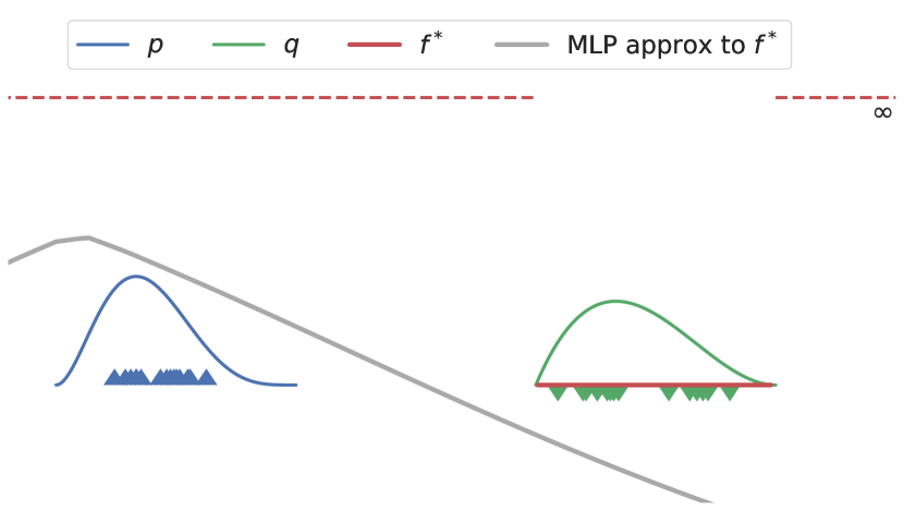
(a) KL divergence optimal critic $f^{*}=\frac{p}{q}$
and smooth critic estimate.

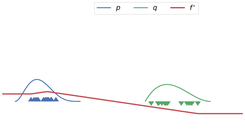
(b) Optimal Wasserstein critic is smooth.

Figure 1: The importance of critic smoothness when estimating divergences and distances. Left: When the two distributions do not have overlapping support, the KL divergence provides no learning signal, while a smooth approximation via a learned critic does. Right: The optimal Wasserstein critic has a smoothness Lipschitz constraint in its definition.

Distributional distances. Including smoothness constraints in the definition of distributional distances by using optimal transport has seen a uptake in machine learning applications in recent years, from generative modeling [52, 13, 58, 59] to reinforcement learning [60, 61], neural ODEs [62] and fairness [63, 64]. Optimal transport is connected to Lipschitz smoothness as the Wasserstein distance can be computed via the Kantorovich-Rubinstein duality [65]:

$$W_{1}(p(\mathbf{x}),q(\mathbf{x}))=\sup_{f:\left\lVert f\right\rVert_{\text{Lip}}\leq 1}\mathbb{E}_{p(\mathbf{x})}f(\mathbf{x})-\mathbb{E}_{q(\mathbf{x})}f(\mathbf{x})$$ (5)

The Wasserstein distance is finding the critic that can separate the two distributions in expectation, but constraints that critic to be Lipschitz in order to avoid pathological solutions. The importance of the Lipschitz constraint on the critic can be seen in Figure 1(b): unlike the KL divergence, the optimal Wasserstein critic is well defined when the two distributions do not have overlapping support, and does not require an approximation to provide useful learning signal for a generative model.

5 Consequences of poor smoothness assumptions

Weak models. Needlessly limiting the capacity of our models by enforcing smoothness constraints is a significant danger: a constant function is very smooth, but not very useful. Beyond trivial examples, Jacobsen et al. [66] show that one of the reasons neural networks are vulnerable to adversarial perturbations is invariance to task relevant changes - too much smoothness with respect to the wrong metric. A neural network can be “too Lipschitz”: methods aimed at increasing robustness to adversarial examples do indeed decrease the Lipschitz constant of a classifier, but once the Lipschitz constant becomes too low, accuracy drops significantly [67].

There are two main avenues for being too restrictive in the specification of smoothness constraints, depending on where and how smoothness is encouraged. Smoothness constraints can be imposed on the entire input space or only in certain pockets, often around the data distribution. Methods which impose constraints on the entire space throw away useful information about the input distribution and restrict the learned function needlessly by forcing it to be smooth in areas of the space where there is no data. This is especially problematic when the input lies on a small manifold in a large dimensional space, such as in the case of natural images, which are a tiny fraction of the space of all possible images. Model capacity can also be needlessly restrained by imposing strong constraints on the individual components of the model, often the network layers, instead of allowing the network to allocate capacity as needed.

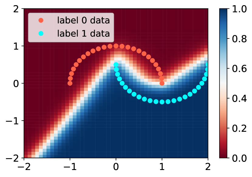
(a) 2 layer MLP.

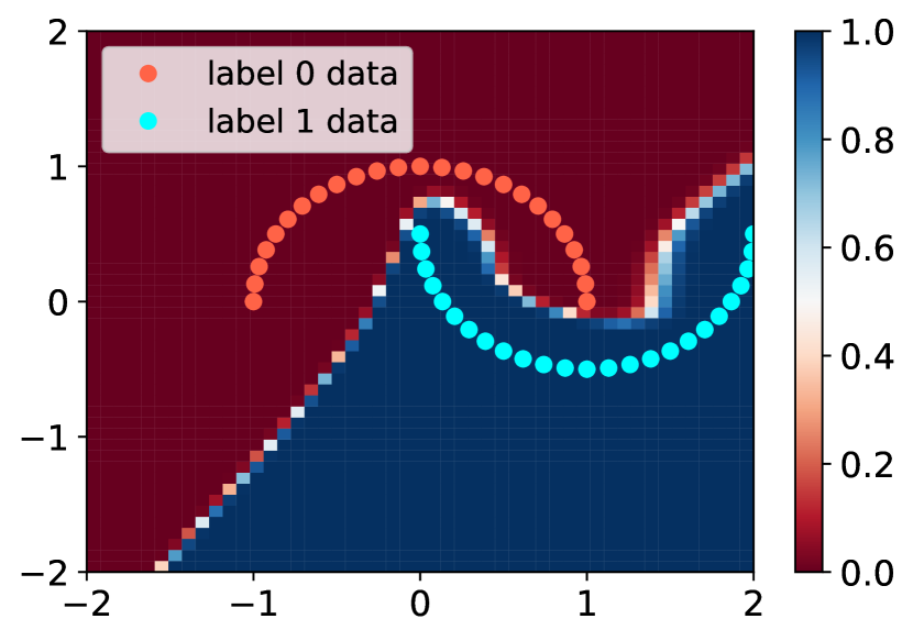
(b) 4 layer MLP.

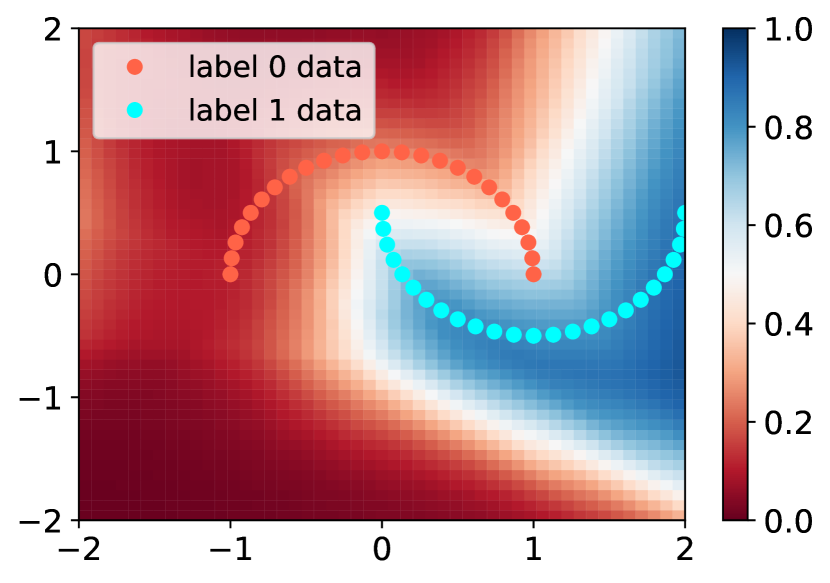
(c) Gradient penalty at data; $K=1$.

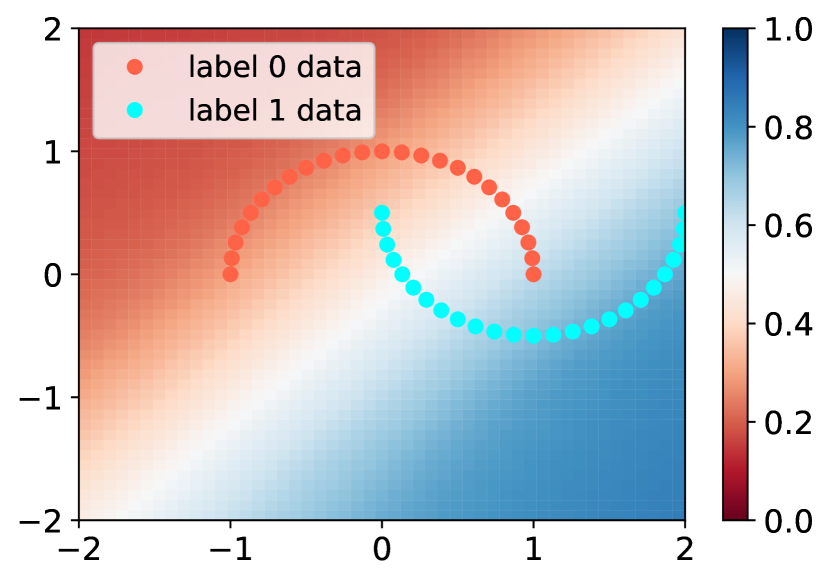
(d) Spectral norm;
$K=1$.

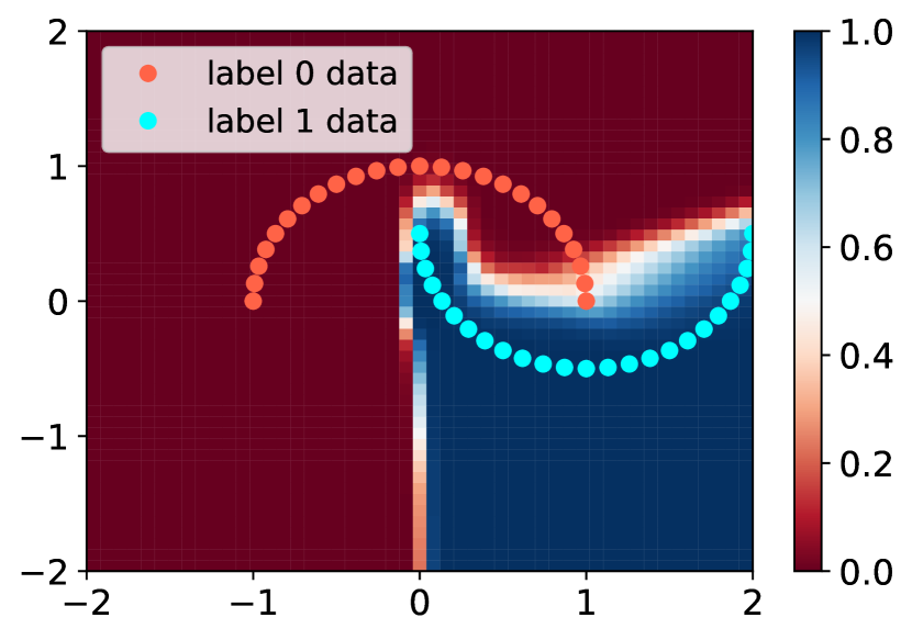
(e) Spectral norm;
$K=10$.

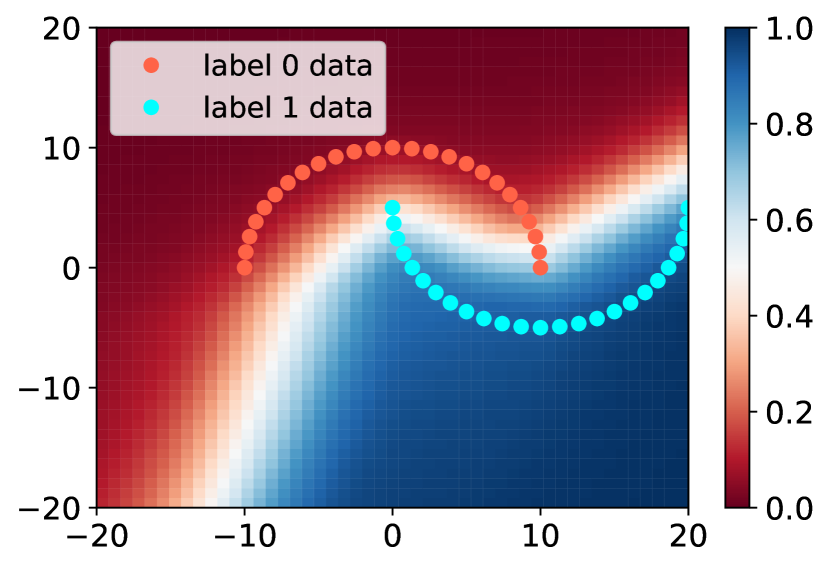
(f) Spectral norm;
scaling the data by 10.

Figure 2: Decision surfaces on two moons under different regularization methods.
Unless otherwise specified the model architecture is a 4 layer MLP.

We can exemplify the importance of where and how constraints are imposed with an example, by contrasting gradient penalties - end to end regularization applied around the training data - and Spectral Normalization - layerwise regularization applied to the entire space. Figure 2(d) shows that using Spectral Normalization to restrict the Lipschitz constant of an MLP to be 1 decreases the capacity of the network and severely affects accuracy compared to the baseline MLP - Figure 2(b) - or the MLP regularized using gradient penalties - Figure 2(c). Further insight comes from Figure 3, which shows that the gradient penalty only enforces a weak constraint on the model and does not heavily restrict the spectral norms of individual layers; this is in stark contrast with Spectral Normalization which by construction ensures each network layer has spectral norm equal to 1. To show the effect of data dependent regularization on local smoothness we plot the Lipschitz constants of the model at neighborhoods spanning the entire space in Figure 4. Each Lipschitz constant is computed using an exhaustive grid search inside each local neighborhood rather than a bound - details are provided in Appendix A.1. As expected, gradient penalties impose stronger constraints around the training data, while Spectral Normalization has a strong effect on the smoothness around points in the entire space. This simple example suggests that the search for better smoothness priors needs to investigate where we want functions to be smooth and reexamine how smoothness constraints should account for the compositional aspect of neural networks, otherwise we run the risk of learning trivially smooth functions.

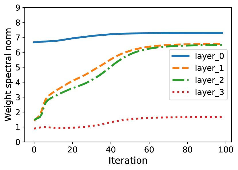
(a) Unregularized.

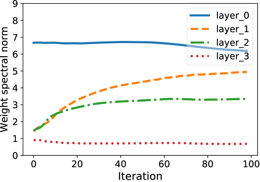
(b) Gradient penalty. $K=1$.

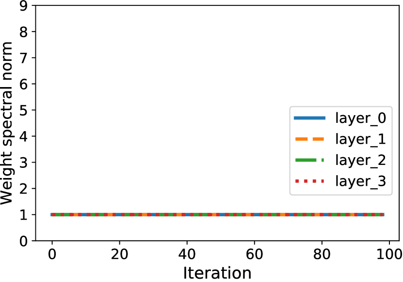
(c) Spectral Normalization. $K=1$.

Figure 3: Lipschitz constant of each layer of an MLP trained on the two moons dataset.
The decision surfaces for the same models can be seen in Figure 2. Smaller means smoother.

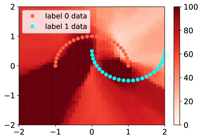
(a) Unregularized.

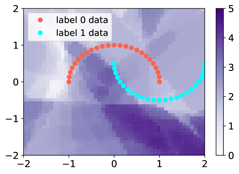
(b) Gradient penalty. $K=1$.

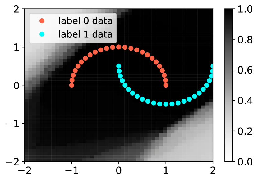
(c) Spectral Normalization. $K=1$.

Figure 4: The effect of regularization on local smoothness. We plot the local Lipschitz constants obtained this using an exhaustive grid search in local neighborhoods, instead of loose bounds. We use different colors to emphasize the different scale of the constants for the different methods.

Overlooked interactions with optimization. We show that viewing smoothness only through the lens of the model is misleading, as smoothness constraints have a strong effect on optimization. The interaction between smoothness and optimization has been mainly observed when training generative models; encouraging the smoothness of the encoder through spectral regularization increased the stability of hierarchical VAEs and led variational inference models to the state of the art of explicit likelihood non autoregressive models [45], while smoothness regularization of the critic (or discriminator) has been established as an indispensable stabilizer of GAN training, independently of the training criteria used [4, 15, 14, 41, 68].

Some smoothness regularization techniques affect optimization by changing the loss function (gradient penalties, spectral regularization) or the optimization regime directly (early stopping, projection methods). Even if they don’t explicitly change the loss function or optimization regime, smoothness constraints affect the path the model takes to reach convergence. We use a simple example to show why smoothness regularization interacts with optimization in Figure 5a. We use different learning rates to train two unregularized MLP classifiers on MNIST [69] and observe that the learning rate used affects its smoothness throughout training, without changing testing accuracy. This shows that imposing similar smoothness constraints on two models which share the same architecture but are trained with different learning rates would lead to very different strengths of regularization and drastically change the trajectory of optimization.

Beyond learning rates, smoothness constraints also interact with momentum. In the GAN setting, Gulrajani et al. [13] observed that weight clipping in the Wasserstein GAN critic requires low to no momentum. Weight clipping has since been abandoned in the favour of other methods, but as we show in Figure 5b and Appendix A.1 current methods like Spectral Normalization applied to GAN critics trained with low momentum decrease sensitivity to learning rates but perform poorly in conjunction with high momentum, leading to slower convergence and higher hyperparameter sensitivity.

We have shown that smoothness constraints interact with optimization parameters such as learning rates and momentum, and argue that we need to reassess our understanding of smoothness constraints, not only as constraints on the final model, but as methods which influence the optimization path.

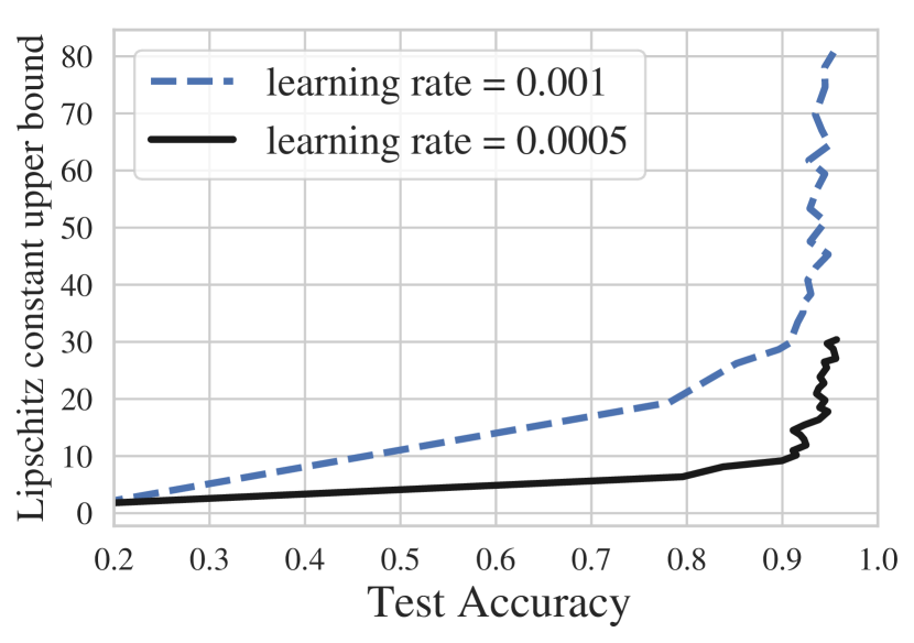
a MNIST classification.

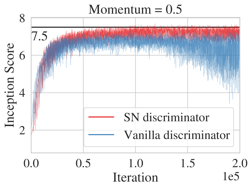
b Spectral Normalization requires low momentum in GAN training.

Figure 5: Smoothness interacts with optimization. Left: MNIST classifiers trained with different learning rates exhibit different smoothness behaviour throughout training, even at the same test accuracy. Lower means smoother. Right: The effects of momentum on Spectral Normalization applied to the GAN discriminator on CIFAR-10. Higher is better.

Sensitivity to data scaling. Sensitivity to data scaling of smoothness constraints can make training neural network models sensitive to additional hyperparameters. Let $f^{*}$ be the optimal decision function for a task obtained from using i.i.d samples from random variable $X$, and $f_{c}^{*}$ obtained similarly from i.i.d samples obtained from $cX$. Since $f^{*}$ and $f_{c}^{*}$ can be highly non linear, the relationship between the smoothness of the two functions is unclear. This gets further complicated when we consider their closest approximators under a neural family. The effect of data scaling on the smooth constraints required to fit a model can be exemplified using the two moons dataset: with a Lipschitz constraint of 1 on the model the data is poorly fit - Figure 2(d) - but a much better fit can be obtained by changing the Lipschitz constant to 10 - Figure 2(e) - or scaling the data - Figure 2(f).

Wrong model priors. The wrong kind of smooth functions can have a similar effect to restricting capacity by introducing the wrong inductive biases. For many regularization techniques it is unclear what kind of smoothness they are encouraging and how strong their effect is on the smoothness of the learned function. Lipschitz smoothness constraints on image models are often specified with respect to the $l_{2}$ norm, which is notorious for not being a meaningful distance metric for natural images. Why are we using the power of feature learning if we are restricting our models to be part of a family of functions which impose constraints that rely on rigid distance metrics? We have seen that smooth critics can be a catalyst for learning by providing the right signal, but that is only if their similarity measures are relevant for the task.

6 Paving the path towards smoothness in neural networks

Smoothness regularization of neural networks has brought forward advances in a plethora of machine learning tasks, from supervised to unsupervised and reinforcement learning. These advances are just scratching the surface of the benefits of smoothness, to explore its full potential we have to use new smoothness definitions, distance metrics and complexity measures; we need to define task and modality dependent smoothness constraints applied to learned representations; we have to adopt an integrated view and understand its interactions with losses, data, model architectures and optimization. Meanwhile, in the world of task agnostic smoothness applied to high dimensional data spaces, we continue to be surprised that specifying smoothness constraints is not better.

New ways of defining smoothness. Improving model generalization and robustness requires specifying the right level of invariance by using task information to define smoothness constraints. To solve issues in generative modelling such as “mode dropping” or “mode collapse”, where entire modes from the data distribution are not captured by the model, we have to go beyond current smoothness measures such as Lipschitz continuity defined on the input space. With the right feature space, images of cats are close to images of dogs, and thus a model which is smooth in that space is less likely to drop one of the two modes. We have to ask what are the desired properties of $h$ such that $\left\lVert f(h(\mathbf{x}))-f(h(\mathbf{y}))\right\rVert\leq\left\lVert h(\mathbf{x})-h(\mathbf{y})\right\rVert$ instead of applying the smoothness constraints on the raw data. Since we require that the mapping $h$ does not discard task relevant information in the data, maintains useful diversity and accounts for input modalities, it has to be data and task dependent. As we have seen again and again in the development of machine learning, handcrafting $h$ is not a scalable solution, and thus the mapping itself has to be learned. Since the approaches used for learning the right representations have to be task dependent, different insights will be required for supervised and unsupervised methods. We expect that semi-supervised learning will play an important role, and that hints for useful properties of representation domains will come from representation learning methods and inference techniques.

New ways of measuring smoothness. Measuring smoothness of a function parametrized by a neural network is challenging even for the most common measure of smoothness used in machine learning, Lipschitzness. Loose upper and lower bounds which rely on function composition are often used [70, 71].  Fazlyab et al. [67] provide an algorithm with tighter bounds by leveraging that activation functions are derivatives of convex functions and cast finding the Lipschitz constant as the result of a convex optimization problem. However, their most accurate approach scales quadratically with the number of neurons and only applies to feed forward networks.  Sokolić et al. [12] provide an upper bound for the Lipschitz constant of a neural network with linear, softmax and pooling layers restricted to input space $\mathcal{X}$ via $\left\lVert f(\mathbf{x})-f(\mathbf{y})\right\rVert_{2}\leq\sup_{\mathbf{z}\in\text{convex\_hull}(\mathcal{X})}J(\mathbf{z})\left\lVert\mathbf{x}-\mathbf{y}\right\rVert_{2},\hskip 10.00002pt\forall\mathbf{x},\mathbf{y}\in\mathcal{X}$, but empirically resort to layerwise bounds. If we want to understand the effects of network architectures, regularization methods and optimization algorithms have on model smoothness, we have to be able to accurately measure it.

New learning paradigms. Combining non parametric methods with feature learning is a promising approach to learning smooth decision surfaces. Given the right data representations and the appropriate distance metrics, interpolating between training examples is an excellent and interpretable smoothness prior. Pursuing this avenue of research entails learning the right features, which themselves might have to be smooth [30], as well as further avenues for scaling non parametric methods such as Gaussian Processes, Support Vector Machines and Nearest Neighbours methods to large datasets.

New measures of model complexity. Standard complexity measures, from VC dimensions and Rademacher complexity, to simpler measures such as number of learned parameters ignore the problem the model has to solve. Task definitions need to be accounted for in the new generation of model complexity measures, since fitting random labels (as per Rademacher complexity) discounts the inductive bias in smoothness constraints that can help model fitting and generalization. The issue of measuring model complexity is inherently tied with many other issues discussed so far, such as choosing ways to define and quantify smoothness.

New approaches to old problems. Smooth learned critics have advanced the state of art in generative modeling and reinforcement learning. Why stop there? By viewing parametric critics as learned loss functions, and observing that for any lower layer of a neural network the upper layers are part of a learned loss function, we can further explore and expand the benefits of smoothness. By exploring how smoothness helps critics in non stationary environments such as reinforcement learning and generative models, we can solve notorious neural network training problems such as covariate shift.

Acknowledgments. We would like to thank Suman Ravuri for helpful comments and discussions.

Appendix A Appendix

A.1 Additional experimental results and experimental methodology

Architectures. In all the two moons experiments, the DeepMLP has 4 layers and 100, 100, 100 and 1 output units respectively. The shallow MLP has 2 layers of 100 and 1 unit. All methods were trained for 100 iterations on 50 datapoints. The MNIST plots are obtained from MLP classifiers having 4 layers of 1000, 1000, 1000 and 10 units each and are trained for 500 iterations at batch size 100, reaching an accuracy of 95% on the entire test set. For the GAN CIFAR-10 experiments, we use the architectures specified in the Spectral normalization paper [5]. Unless otherwise specified, we use the default Adam optimizer [72] $\beta_{1}$ and $\beta_{2}$ parameters.

Computing the local Lipschitz constant in Figure 4. To compute the local Lipschitz function of the decision surface learned on two moons, we split the space into small neighborhoods (2500 equally sized grids). For each grid, we sample 2500 random pairs of points in the grid and report $\max\left\lVert f(\mathbf{x})-f(\mathbf{y})\right\rVert/\left\lVert\mathbf{x}-\mathbf{y}\right\rVert$.

Spectral normalization. In Figure 6 we show that the effect of momentum on spectral normalization is independent of whether caching of the initialization vector for power iteration is performed or not.

(a) Low momentum: 0.5.

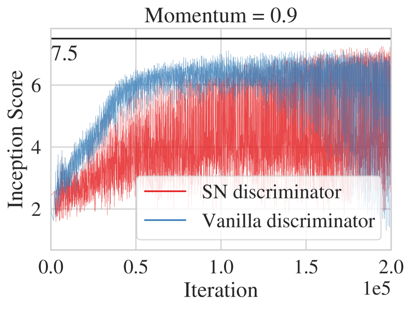
(b) High momentum: 0.9.

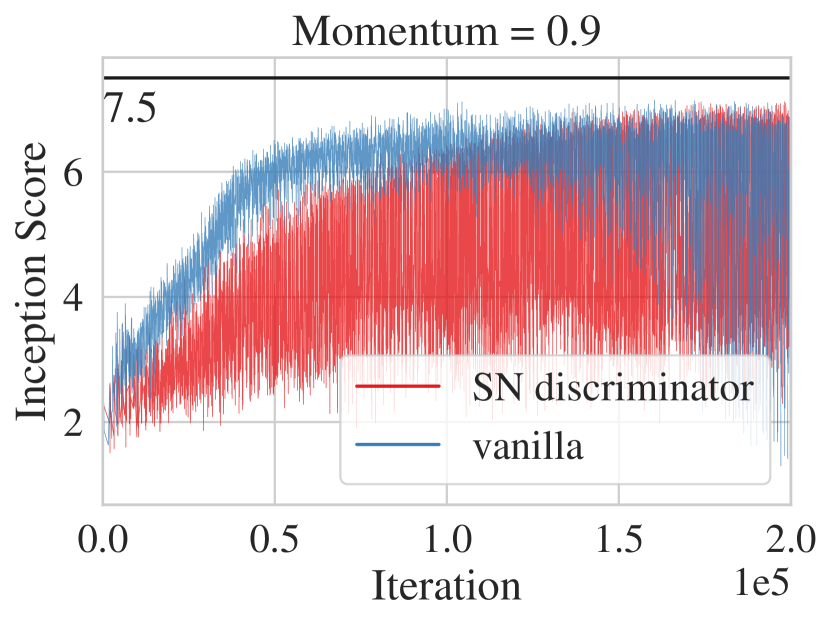
(c) High momentum with 10 power iteration caching and no caching.

Figure 6: The effect of momentum on spectral normalization on GAN performance. This shows that the iteration between momentum and spectral normalization is not due to the caching between iterations done for computational reasons.

References

- Ioffe and Szegedy [2015] Sergey Ioffe and Christian Szegedy. Batch normalization: Accelerating deep network training by reducing internal covariate shift. In International Conference on Machine Learning, pages 448–456, 2015.
- Srivastava et al. [2014] Nitish Srivastava, Geoffrey Hinton, Alex Krizhevsky, Ilya Sutskever, and Ruslan Salakhutdinov. Dropout: a simple way to prevent neural networks from overfitting. The journal of machine learning research, 15(1):1929–1958, 2014.
- Loshchilov and Hutter [2018] Ilya Loshchilov and Frank Hutter. Decoupled weight decay regularization. In International Conference on Learning Representations, 2018.
- Yoshida and Miyato [2017] Yuichi Yoshida and Takeru Miyato. Spectral norm regularization for improving the generalizability of deep learning. arXiv preprint arXiv:1705.10941, 2017.
- Miyato et al. [2018] Takeru Miyato, Toshiki Kataoka, Masanori Koyama, and Yuichi Yoshida. Spectral normalization for generative adversarial networks. In International Conference on Learning Representations, 2018.
- Gouk et al. [2020] Henry Gouk, Eibe Frank, Bernhard Pfahringer, and Michael J Cree. Regularisation of neural networks by enforcing lipschitz continuity. Machine Learning, pages 1–24, 2020.
- Kim et al. [2020] Hyunjik Kim, George Papamakarios, and Andriy Mnih. The lipschitz constant of self-attention. arXiv preprint arXiv:2006.04710, 2020.
- Tsuzuku et al. [2018] Yusuke Tsuzuku, Issei Sato, and Masashi Sugiyama. Lipschitz-margin training: Scalable certification of perturbation invariance for deep neural networks. In Advances in neural information processing systems, pages 6541–6550, 2018.
- Cisse et al. [2017] Moustapha Cisse, Piotr Bojanowski, Edouard Grave, Yann Dauphin, and Nicolas Usunier. Parseval networks: improving robustness to adversarial examples. In Proceedings of the 34th International Conference on Machine Learning-Volume 70, pages 854–863, 2017.
- Bartlett et al. [2018] Peter L Bartlett, Steven N Evans, and Philip M Long. Representing smooth functions as compositions of near-identity functions with implications for deep network optimization. arXiv preprint arXiv:1804.05012, 2018.
- He et al. [2016] Kaiming He, Xiangyu Zhang, Shaoqing Ren, and Jian Sun. Deep residual learning for image recognition. In Proceedings of the IEEE conference on computer vision and pattern recognition, pages 770–778, 2016.
- Sokolić et al. [2017] Jure Sokolić, Raja Giryes, Guillermo Sapiro, and Miguel RD Rodrigues. Robust large margin deep neural networks. IEEE Transactions on Signal Processing, 65(16):4265–4280, 2017.
- Gulrajani et al. [2017] Ishaan Gulrajani, Faruk Ahmed, Martin Arjovsky, Vincent Dumoulin, and Aaron C Courville. Improved training of wasserstein gans. In Advances in neural information processing systems, pages 5767–5777, 2017.
- Fedus et al. [2018] William Fedus, Mihaela Rosca, Balaji Lakshminarayanan, Andrew M Dai, Shakir Mohamed, and Ian Goodfellow. Many paths to equilibrium: Gans do not need to decrease a divergence at every step. In International Conference on Learning Representations, 2018.
- Arbel et al. [2018] Michael Arbel, Dougal Sutherland, Mikołaj Bińkowski, and Arthur Gretton. On gradient regularizers for mmd gans. In Advances in neural information processing systems, pages 6700–6710, 2018.
- Kodali et al. [2017] Naveen Kodali, Jacob Abernethy, James Hays, and Zsolt Kira. On convergence and stability of gans. arXiv preprint arXiv:1705.07215, 2017.
- Lassance et al. [2018] Carlos Eduardo Rosar Kos Lassance, Vincent Gripon, and Antonio Ortega. Laplacian networks: Bounding indicator function smoothness for neural network robustness. arXiv preprint arXiv:1805.10133, 2018.
- Vapnik [2013] Vladimir Vapnik. The nature of statistical learning theory. Springer science & business media, 2013.
- Novak et al. [2018] Roman Novak, Yasaman Bahri, Daniel A Abolafia, Jeffrey Pennington, and Jascha Sohl-Dickstein. Sensitivity and generalization in neural networks: an empirical study. In International Conference on Learning Representations, 2018.
- Rasmussen and Ghahramani [2001] Carl Edward Rasmussen and Zoubin Ghahramani. Occam’s razor. In Advances in neural information processing systems, pages 294–300, 2001.
- Bartlett [1997] Peter L Bartlett. For valid generalization the size of the weights is more important than the size of the network. In Advances in neural information processing systems, pages 134–140, 1997.
- Golowich et al. [2018] Noah Golowich, Alexander Rakhlin, and Ohad Shamir. Size-independent sample complexity of neural networks. In Conference On Learning Theory, pages 297–299. PMLR, 2018.
- Hardt et al. [2016] Moritz Hardt, Ben Recht, and Yoram Singer. Train faster, generalize better: Stability of stochastic gradient descent. In International Conference on Machine Learning, pages 1225–1234. PMLR, 2016.
- Nakkiran et al. [2019] Preetum Nakkiran, Gal Kaplun, Yamini Bansal, Tristan Yang, Boaz Barak, and Ilya Sutskever. Deep double descent: Where bigger models and more data hurt. In International Conference on Learning Representations, 2019.
- Krizhevsky et al. [2012] Alex Krizhevsky, Ilya Sutskever, and Geoffrey E Hinton. Imagenet classification with deep convolutional neural networks. In Advances in neural information processing systems, pages 1097–1105, 2012.
- Simonyan and Zisserman [2015] Karen Simonyan and Andrew Zisserman. Very deep convolutional networks for large-scale image recognition. In 3rd International Conference on Learning Representations, 2015.
- Jun et al. [2020] Heewoo Jun, Rewon Child, Mark Chen, John Schulman, Aditya Ramesh, Alec Radford, and Ilya Sutskever. Distribution augmentation for generative modeling. In Proceedings of the 37th International Conference on Machine Learning, volume 119 of Proceedings of Machine Learning Research, pages 5006–5019, 2020.
- Belkin et al. [2019] Mikhail Belkin, Daniel Hsu, Siyuan Ma, and Soumik Mandal. Reconciling modern machine-learning practice and the classical bias–variance trade-off. Proceedings of the National Academy of Sciences, 116(32):15849–15854, 2019.
- van Amersfoort et al. [2020] Joost van Amersfoort, Lewis Smith, Yee Whye Teh, and Yarin Gal. Simple and scalable epistemic uncertainty estimation using a single deep deterministic neural network. International Conference on Machine Learning, 2020.
- Liu et al. [2020] Jeremiah Zhe Liu, Zi Lin, Shreyas Padhy, Dustin Tran, Tania Bedrax-Weiss, and Balaji Lakshminarayanan. Simple and principled uncertainty estimation with deterministic deep learning via distance awareness. arXiv preprint arXiv:2006.10108, 2020.
- Lakshminarayanan et al. [2017] Balaji Lakshminarayanan, Alexander Pritzel, and Charles Blundell. Simple and scalable predictive uncertainty estimation using deep ensembles. In Advances in neural information processing systems, pages 6402–6413, 2017.
- Szegedy et al. [2013] Christian Szegedy, Wojciech Zaremba, Ilya Sutskever, Joan Bruna, Dumitru Erhan, Ian Goodfellow, and Rob Fergus. Intriguing properties of neural networks. arXiv preprint arXiv:1312.6199, 2013.
- Goodfellow et al. [2015] Ian Goodfellow, Jonathon Shlens, and Christian Szegedy. Explaining and harnessing adversarial examples. In International Conference on Learning Representations, 2015.
- Papernot et al. [2016] Nicolas Papernot, Patrick McDaniel, Somesh Jha, Matt Fredrikson, Z Berkay Celik, and Ananthram Swami. The limitations of deep learning in adversarial settings. In 2016 IEEE European symposium on security and privacy (EuroS&P), pages 372–387. IEEE, 2016.
- Chakraborty et al. [2018] Anirban Chakraborty, Manaar Alam, Vishal Dey, Anupam Chattopadhyay, and Debdeep Mukhopadhyay. Adversarial attacks and defences: A survey. arXiv preprint arXiv:1810.00069, 2018.
- Kurakin et al. [2016] Alexey Kurakin, Ian Goodfellow, and Samy Bengio. Adversarial machine learning at scale. International Conference on Learning Representations, 2016.
- Moosavi-Dezfooli et al. [2017] Seyed-Mohsen Moosavi-Dezfooli, Alhussein Fawzi, Omar Fawzi, and Pascal Frossard. Universal adversarial perturbations. In Proceedings of the IEEE conference on computer vision and pattern recognition, pages 1765–1773, 2017.
- Madry et al. [2018] Aleksander Madry, Aleksandar Makelov, Ludwig Schmidt, Dimitris Tsipras, and Adrian Vladu. Towards deep learning models resistant to adversarial attacks. In International Conference on Learning Representations, 2018.
- Gilmer et al. [2018] Justin Gilmer, Luke Metz, Fartash Faghri, Samuel S Schoenholz, Maithra Raghu, Martin Wattenberg, and Ian Goodfellow. Adversarial spheres. arXiv preprint arXiv:1801.02774, 2018.
- Goodfellow et al. [2014] Ian Goodfellow, Jean Pouget-Abadie, Mehdi Mirza, Bing Xu, David Warde-Farley, Sherjil Ozair, Aaron Courville, and Yoshua Bengio. Generative adversarial nets. In Advances in neural information processing systems, pages 2672–2680, 2014.
- Brock et al. [2018] Andrew Brock, Jeff Donahue, and Karen Simonyan. Large scale gan training for high fidelity natural image synthesis. In International Conference on Learning Representations, 2018.
- de Masson d’Autume et al. [2019] Cyprien de Masson d’Autume, Shakir Mohamed, Mihaela Rosca, and Jack Rae. Training language gans from scratch. In Advances in Neural Information Processing Systems, pages 4300–4311, 2019.
- Kingma and Welling [2014] Diederik P Kingma and Max Welling. Auto-encoding variational bayes. International Conference on Learning Representations, 2014.
- Rezende et al. [2014] Danilo Jimenez Rezende, Shakir Mohamed, and Daan Wierstra. Stochastic backpropagation and approximate inference in deep generative models. In International Conference on Machine Learning, pages 1278–1286, 2014.
- Vahdat and Kautz [2020] Arash Vahdat and Jan Kautz. Nvae: A deep hierarchical variational autoencoder. Advances in Neural Information Processing Systems, 33, 2020.
- Rezende and Mohamed [2015] Danilo Rezende and Shakir Mohamed. Variational inference with normalizing flows. In International Conference on Machine Learning, pages 1530–1538, 2015.
- Behrmann et al. [2019] Jens Behrmann, Will Grathwohl, Ricky TQ Chen, David Duvenaud, and Jörn-Henrik Jacobsen. Invertible residual networks. In International Conference on Machine Learning, pages 573–582, 2019.
- Nguyen et al. [2010] XuanLong Nguyen, Martin J Wainwright, and Michael I Jordan. Estimating divergence functionals and the likelihood ratio by convex risk minimization. IEEE Transactions on Information Theory, 56(11):5847–5861, 2010.
- Nowozin et al. [2016] Sebastian Nowozin, Botond Cseke, and Ryota Tomioka. f-gan: Training generative neural samplers using variational divergence minimization. In Advances in neural information processing systems, pages 271–279, 2016.
- Arbel et al. [2020] Michael Arbel, Liang Zhou, and Arthur Gretton. Kale: When energy-based learning meets adversarial training. arXiv preprint arXiv:2003.05033, 2020.
- Schäfer et al. [2019] Florian Schäfer, Hongkai Zheng, and Anima Anandkumar. Implicit competitive regularization in gans. arXiv preprint arXiv:1910.05852, 2019.
- Arjovsky et al. [2017] Martin Arjovsky, Soumith Chintala, and Léon Bottou. Wasserstein generative adversarial networks. In Proceedings of the 34th International Conference on Machine Learning-Volume 70, pages 214–223, 2017.
- Zhou et al. [2019] Zhiming Zhou, Jiadong Liang, Yuxuan Song, Lantao Yu, Hongwei Wang, Weinan Zhang, Yong Yu, and Zhihua Zhang. Lipschitz generative adversarial nets. In International Conference on Machine Learning, pages 7584–7593, 2019.
- Belghazi et al. [2018] Mohamed Ishmael Belghazi, Aristide Baratin, Sai Rajeswar, Sherjil Ozair, Yoshua Bengio, Aaron Courville, and R Devon Hjelm. Mine: mutual information neural estimation. arXiv preprint arXiv:1801.04062, 2018.
- Oord et al. [2018] Aaron van den Oord, Yazhe Li, and Oriol Vinyals. Representation learning with contrastive predictive coding. arXiv preprint arXiv:1807.03748, 2018.
- Tschannen et al. [2020] Michael Tobias Tschannen, Josip Djolonga, Paul Kishan Rubenstein, Sylvain Gelly, and Mario Lučić. On mutual information maximization for representation learning. In International Conference on Learning Representations, 2020.
- D’Oro and Jaśkowski [2020] Pierluca D’Oro and Wojciech Jaśkowski. How to learn a useful critic? model-based action-gradient-estimator policy optimization. arXiv preprint arXiv:2004.14309, 2020.
- Tolstikhin et al. [2018] Ilya Tolstikhin, Olivier Bousquet, Sylvain Gelly, and Bernhard Schoelkopf. Wasserstein auto-encoders. International Conference on Learning Representations, 2018.
- Ostrovski et al. [2018] Georg Ostrovski, Will Dabney, and Remi Munos. Autoregressive quantile networks for generative modeling. In International Conference on Machine Learning, pages 3936–3945, 2018.
- Bellemare et al. [2017] Marc G Bellemare, Will Dabney, and Rémi Munos. A distributional perspective on reinforcement learning. In International Conference on Machine Learning, pages 449–458, 2017.
- Dabney et al. [2018] Will Dabney, Georg Ostrovski, David Silver, and Remi Munos. Implicit quantile networks for distributional reinforcement learning. In International Conference on Machine Learning, pages 1096–1105, 2018.
- Finlay et al. [2020] Chris Finlay, Jörn-Henrik Jacobsen, Levon Nurbekyan, and Adam M Oberman. How to train your neural ode. International Conference on Machine Learning, 2020.
- Silvia et al. [2020] Chiappa Silvia, Jiang Ray, Stepleton Tom, Pacchiano Aldo, Jiang Heinrich, and Aslanides John. A general approach to fairness with optimal transport. Proceedings of the AAAI Conference on Artificial Intelligence, 34(04):3633–3640, Apr. 2020.
- Jiang et al. [2020] Ray Jiang, Aldo Pacchiano, Tom Stepleton, Heinrich Jiang, and Silvia Chiappa. Wasserstein fair classification. In Uncertainty in Artificial Intelligence, pages 862–872. PMLR, 2020.
- Villani [2008] C. Villani. Optimal Transport: Old and New. Grundlehren der mathematischen Wissenschaften. Springer Berlin Heidelberg, 2008. ISBN 9783540710509. URL https://books.google.ch/books?id=hV8o5R7_5tkC.
- Jacobsen et al. [2018] Joern-Henrik Jacobsen, Jens Behrmann, Richard Zemel, and Matthias Bethge. Excessive invariance causes adversarial vulnerability. In International Conference on Learning Representations, 2018.
- Fazlyab et al. [2019] Mahyar Fazlyab, Alexander Robey, Hamed Hassani, Manfred Morari, and George Pappas. Efficient and accurate estimation of lipschitz constants for deep neural networks. In Advances in Neural Information Processing Systems, pages 11427–11438, 2019.
- Kurach et al. [2019] Karol Kurach, Mario Lučić, Xiaohua Zhai, Marcin Michalski, and Sylvain Gelly. A large-scale study on regularization and normalization in gans. In International Conference on Machine Learning, pages 3581–3590. PMLR, 2019.
- LeCun et al. [1999] Yann LeCun, Patrick Haffner, Léon Bottou, and Yoshua Bengio. Object recognition with gradient-based learning. In Shape, contour and grouping in computer vision, pages 319–345. Springer, 1999.
- Virmaux and Scaman [2018] Aladin Virmaux and Kevin Scaman. Lipschitz regularity of deep neural networks: analysis and efficient estimation. In Advances in Neural Information Processing Systems, pages 3835–3844, 2018.
- Combettes and Pesquet [2019] Patrick L Combettes and Jean-Christophe Pesquet. Lipschitz certificates for neural network structures driven by averaged activation operators. arXiv preprint arXiv:1903.01014, 2019.
- Kingma and Ba [2015] Diederik P Kingma and Jimmy Ba. Adam: A method for stochastic optimization. International Conference on Learning Representations, 2015.