Template Matching with Ranks

Ery Arias-Castro    Lin Zheng
Abstract

We consider the problem of matching a template to a noisy signal. Motivated by some recent proposals in the signal processing literature, we suggest a rank-based method and study its asymptotic properties using some well-established techniques in empirical process theory combined with Hájek’s projection method. The resulting estimator of the shift is shown to achieve a parametric rate of convergence and to be asymptotically normal. Some numerical simulations corroborate these findings.

The authors are with the Department of Mathematics, University of California, San Diego, USA. Contact information is available here and here.

Keywords: matched filter, template matching, scan statistics, Spearman rank correlation, empirical processes, minimax optimality

1 Introduction

Template matching is the process of matching a clean and noiseless template to an observed, typically noisy signal. This topic is closely related to the problem of matching two or more noisy signals, sometimes referred to as ‘aligning’ or ‘registering’ the signals, and to methodology in spatial statistics falling under the umbrella name of ‘scan statistic’. When the template has a point of discontinuity, matching a template to the signal can be interpreted as detecting the location of the discontinuity, a more specialized task more broadly referred to as ‘change-point detection’ in statistics. For pointers to the vast literature on these related topics, we refer the reader to the introduction of another recent paper of ours on the topic (Arias-Castro and Zheng, 2020).

While in our previous work we proposed and analyzed M-estimators for template matching, in the present paper we consider R-estimators instead. The former includes what is perhaps the most widely used method which consists in maximizing the Pearson correlation of the signal with a shift of the template; see (2) below. We focus here on the rank variant of this approach, which is an example of the latter category and consists, instead, in replacing the signal with the corresponding ranks before maximizing the correlation over shifts of the template; see (4).

Rank-based methods are, of course, classical in statistics (Šidák et al., 1999; Hettmansperger and McKean, 2010; Lehmann, 2006; Gibbons and Chakraborti, 2011). The theory of rank tests is particularly well-developed, featuring some prominent methods such as the Wilcoxon/Mann–Whitney and Kruskal–Wallis two- and multi-sample tests, and essentially all (other) distribution-free tests for goodness-of-fit such as the Kolmogorov–Smirnov test, and more closely related to our topic here, the Spearman and Kendall rank correlation tests for independence. The theory of rank estimators, sometimes called R-estimators, is also well developed, although perhaps not as well-known (Hettmansperger and McKean, 2010). The most famous example may be the Hodges–Lehmann estimator, which is derived from the Wilcoxon signed-rank test. In multiple linear regression, the asymptotic linearity and resulting normality of certain R-estimators is established in a number of publications (Jurečková, 1971; Heiler and Willers, 1988; Koul and Mukherjee, 1993; Giraitis et al., 1996; Draper, 1988). Closer to our setting, some papers consider the use of ranks for the detection and/or localization of one or multiple change-points (Darkhovskh, 1976; Gombay and Hušková, 1998; Hušková, 1997; Lung-Yut-Fong et al., 2015; Gerstenberger, 2018; Wang et al., 2020; Arias-Castro et al., 2018).

In the signal and image processing literature per se, where a lot of the work on template matching resides, rank-based methods have been attracting some attention in recent years. Kordelas and Daras (2009) propose a rank variant of the well-known feature extractor SIFT, while Xiong et al. (2020) propose a rank-based local self-similarity feature descriptor for use in synthetic-aperture radar (SAR) imaging. Ayinde and Yang (2002) present a face recognition approach using the rank correlation of Gabor filtered images, while Galea and Farrugia (2016) apply the Spearman rank correlation for template matching in face photo-sketch recognition. Kong et al. (2008) construct a matched-filter object detection algorithm based on the Spearman rank correlation to detect Ca2+ sparks in biochemical applications. A number of papers use ranks to align images, a task also known as ‘stereo matching’ (Banks and Bennamoun, 2001; Banks et al., 1999; Chen et al., 2012; Geng and Gou, 2012) — a problem we will not address here but which also has a sizable literature in statistics; we provide some pointers to the literature in our recent paper (Arias-Castro and Zheng, 2020).

1.1 Model and methods

We consider a standard model for template matching, where we observe a shift of the template with additive noise,

Yi=f(xiθ)+Zi,i=1,,n,formulae-sequencesubscript𝑌𝑖𝑓subscript𝑥𝑖superscript𝜃subscript𝑍𝑖𝑖1𝑛Y_{i}=f(x_{i}-\theta^{*})+Z_{i},\quad i=1,\dots,n, (1)

where xi:=i/nassignsubscript𝑥𝑖𝑖𝑛x_{i}:=i/n denote the design points, f:[0,1]:𝑓01f:[0,1]\to\mathbb{R} is a known 1-periodic function referred to as the template, and θsuperscript𝜃\theta^{*}\in\mathbb{R} is the unknown shift of interest. The noise or measurement error variables Z1,,Znsubscript𝑍1subscript𝑍𝑛Z_{1},\dots,Z_{n} are assumed iid with density ϕitalic-ϕ\phi and distribution function denoted ΦΦ\Phi.

Assumption 1.

We assume everywhere that f𝑓f is 1-periodic, and in fact exactly so in the sense that f(θ)f(θ)f(\cdot-\theta)\neq f(\cdot-\theta^{*}) on a set of positive measure whenever θθmod1𝜃modulosuperscript𝜃1\theta\neq\theta^{*}\!\mod 1. We also assume that f𝑓f is Lipschitz continuous.

Assumption 2.

We assume everywhere that ϕitalic-ϕ\phi is even, so that the noise is symmetric about 0.

Our goal is, in signal processing terminology, to match the template f𝑓f to the signal Y𝑌Y, which in statistical terms consists in the estimation of the shift θsuperscript𝜃\theta^{*}. One of the most popular ways to do so is via maximization of the Pearson correlation, leading to the estimator

θ^:=argmaxθi=1nYif(xiθ).assign^𝜃subscriptargmax𝜃superscriptsubscript𝑖1𝑛subscript𝑌𝑖𝑓subscript𝑥𝑖𝜃\hat{\theta}:=\operatorname*{arg\,max}_{\theta}\sum_{i=1}^{n}Y_{i}\,f(x_{i}-\theta). (2)

In the present context, this is equivalent to the least squares estimator in that the same estimator is also the solution to the following least squares problem

θ^=argminθi=1n(Yif(xiθ))2.^𝜃subscriptargmin𝜃superscriptsubscript𝑖1𝑛superscriptsubscript𝑌𝑖𝑓subscript𝑥𝑖𝜃2\hat{\theta}=\operatorname*{arg\,min}_{\theta}\sum_{i=1}^{n}(Y_{i}-f(x_{i}-\theta))^{2}. (3)

Note that this corresponds to the maximum likelihood estimator when the noise distribution is Gaussian. Of course, other loss functions can be used, some of them leading to methods that are robust to noise distributions with heavy tails or to the presence of gross errors (outliers) in the signal. Our recent paper (Arias-Castro and Zheng, 2020) studies these so-called M-estimators in great detail.

In the present paper we consider, instead, estimators based on ranks. These go by the name of R-estimators in the statistics literature. The most direct route to such an estimator is to replace the response values with their ranks, yielding

θ^rank:=argmaxθi=1nRif(xiθ),assignsubscript^𝜃ranksubscriptargmax𝜃superscriptsubscript𝑖1𝑛subscript𝑅𝑖𝑓subscript𝑥𝑖𝜃\hat{\theta}_{\rm rank}:=\operatorname*{arg\,max}_{\theta}\sum_{i=1}^{n}R_{i}\,f(x_{i}-\theta), (4)

where Risubscript𝑅𝑖R_{i} denotes the rank of Yisubscript𝑌𝑖Y_{i} in {Y1,,Yn}subscript𝑌1subscript𝑌𝑛\{Y_{1},\dots,Y_{n}\} in increasing order. Doing so is sometimes called the ‘rank transformation’ in the signal processing literature. Note that this is similar in spirit to replacing the Pearson correlation in (2) with the Spearman rank correlation, except that we do not rank the values of the template itself. We find that there is no real reason to want to replace the template values with the corresponding ranks as the template is assumed to be free of noise.

1.2 Content

The rest of the paper is devoted to studying the asymptotic (n𝑛n\to\infty) properties of the estimator we propose in (4), which we will refer to as the R-estimator. In Section 2, we derive some basic results describing the asymptotic behavior of this estimator. In more detail, in Section 2.1 we discuss the consistency of this estimator, which we are not fully able to establish but is clearly supported by computer simulations; in Section 2.2 we derive a rate of convergence for our R-estimator, which happens to be parametric and also minimax optimal; and in Section 2.3 we derive a normal limit distribution of the same estimator, as well as its asymptotic relative efficiency with respect to maximum likelihood estimator under Gaussian noise. Section 3 summarizes the result of some numerical experiments we performed to probe our asymptotic theory in finite samples. Section 4 provides a discussion of possible extensions. The mathematical proofs are gathered in Section 5.

2 Theoretical properties

In this section we study the asymptotic properties of the estimator defined in (4). We first study its consistency in Section 2.1; bound its rate of convergence in Section 2.2; and derive its asymptotic (normal) limit distribution in Section 2.3.

2.1 Consistency

The estimator in (4) can be equivalently defined via

θ^n:=argmaxθM^n(θ),assignsubscript^𝜃𝑛subscriptargmax𝜃subscript^𝑀𝑛𝜃\displaystyle\hat{\theta}_{n}:=\operatorname*{arg\,max}_{\theta}\widehat{M}_{n}(\theta), M^n(θ):=1ni=1nRinf(xiθ),assignsubscript^𝑀𝑛𝜃1𝑛superscriptsubscript𝑖1𝑛subscript𝑅𝑖𝑛𝑓subscript𝑥𝑖𝜃\displaystyle\widehat{M}_{n}(\theta):=\frac{1}{n}\sum_{i=1}^{n}\frac{R_{i}}{n}f(x_{i}-\theta), (5)

where we have added the subscript n𝑛n to emphasize that the estimator is being computed on a sample of size n𝑛n. To understand the large-sample behavior of this estimator, we need to understand that of M^nsubscript^𝑀𝑛\widehat{M}_{n} as a function of θ𝜃\theta, and this leads directly to empirical process theory.

Lemma 2.1.

In probability,

supθ|M^n(θ)M(θ)|n0,𝑛subscriptsupremum𝜃subscript^𝑀𝑛𝜃𝑀𝜃0\displaystyle\sup_{\theta\in\mathbb{R}}\big{|}\widehat{M}_{n}(\theta)-M(\theta)\big{|}\xrightarrow{n\to\infty}0,

where

M(θ):=0101Φ2(f(x0)f(x))f(x0+θθ)dxdx0,assign𝑀𝜃superscriptsubscript01superscriptsubscript01subscriptΦ2𝑓subscript𝑥0𝑓𝑥𝑓subscript𝑥0superscript𝜃𝜃differential-d𝑥differential-dsubscript𝑥0\displaystyle M(\theta):=\int_{0}^{1}\int_{0}^{1}\Phi_{2}(f(x_{0})-f(x))f(x_{0}+\theta^{*}-\theta){\rm d}x{\rm d}x_{0}, (6)

with Φ2(t):=Φ(t+z)ϕ(z)dz.assignsubscriptΦ2𝑡superscriptsubscriptΦ𝑡𝑧italic-ϕ𝑧differential-d𝑧\Phi_{2}(t):=\int_{-\infty}^{\infty}\Phi(t+z)\phi(z){\rm d}z.

With the uniform convergence of M^nsubscript^𝑀𝑛\widehat{M}_{n} to M𝑀M established in Lemma 2.1, and with the fact that M𝑀M is continuous and 1-periodic, it suffices that θsuperscript𝜃\theta^{*} be the unique maximizer of M𝑀M for the estimator θ^nsubscript^𝜃𝑛\hat{\theta}_{n} defined in (5) to converge to θsuperscript𝜃\theta^{*} in probability, that is, to be consistent (Van der Vaart, 1998, Th 5.7). We are able, under an additional mild assumption on the noise distribution, to prove that θsuperscript𝜃\theta^{*} is a local maximizer of M𝑀M.

Proposition 2.2.

M𝑀M is twice differentiable, with M(θ)=0superscript𝑀superscript𝜃0M^{\prime}(\theta^{*})=0, and if ϕitalic-ϕ\phi is positive everywhere, M′′(θ)<0superscript𝑀′′superscript𝜃0M^{\prime\prime}(\theta^{*})<0, in which case θsuperscript𝜃\theta^{*} is a local maximizer of M𝑀M.

Unfortunately, we are not able to verify that θsuperscript𝜃\theta^{*} is indeed a global maximizer. However, since it is borne out by our numerical experiments (Section 3), we conjecture this is true, possibly under some additional (reasonable) conditions on the model. In the meantime, we formulate this as an assumption, which henceforth forms part of our basic assumptions.

Assumption 3.

θsuperscript𝜃\theta^{*} is the unique maximum point of M𝑀M defined in (6).

Theorem 2.3.

Under the basic assumptions, θ^nsubscript^𝜃𝑛\hat{\theta}_{n} converges in probability to θsuperscript𝜃\theta^{*} as n𝑛n\to\infty.

2.2 Rate of convergence and minimaxity

Besides consistency, we derive the estimator’s rate of convergence in this section. The rate turns out to be parametric, i.e., the convergence of the estimator to the true value of the parameter is in O(n)𝑂𝑛O(\sqrt{n}).

Theorem 2.4.

Under the basic assumptions, θ^nsubscript^𝜃𝑛\hat{\theta}_{n} is n𝑛\sqrt{n}-consistent.

The parametric rate of n𝑛\sqrt{n} happens to be minimax optimal in the present setting. This is established in (Arias-Castro and Zheng, 2020, Cor 3.9) in the context of a random design corresponding to the situation where the design points, instead of being the grid points spanning the unit interval, are generated as an iid sample from the uniform distribution on the unit interval. But similar arguments carry over. We omit details and refer the reader to the discussion in (Arias-Castro and Zheng, 2020, Sec 6.1).

Corollary 2.5.

The R-estimator achieves the minimax rate of convergence.

2.3 Limit distribution and asymptotic relative efficiency

In addition to obtaining a rate of convergence, we are also able to derive the asymptotic distribution, which happens to be normal.

Theorem 2.6.

Under the basic assumptions, strengthened with the assumption that f𝑓f is continuously differentiable, n(θ^nθ)𝑛subscript^𝜃𝑛superscript𝜃\sqrt{n}(\hat{\theta}_{n}-\theta^{*}) converges weakly to the centered normal distribution with variance γ2/M′′(θ)2superscript𝛾2superscript𝑀′′superscriptsuperscript𝜃2\gamma^{2}/M^{\prime\prime}(\theta^{*})^{2}, where

γ2:=01[01(f(x)f(x0))Ξ(f(x)f(x0),z)dx]2ϕ(z)dzdx0,assignsuperscript𝛾2superscriptsubscript01superscriptsubscriptsuperscriptdelimited-[]superscriptsubscript01superscript𝑓𝑥superscript𝑓subscript𝑥0Ξ𝑓𝑥𝑓subscript𝑥0𝑧differential-d𝑥2italic-ϕ𝑧differential-d𝑧differential-dsubscript𝑥0\displaystyle\gamma^{2}:=\int_{0}^{1}\int_{-\infty}^{\infty}\bigg{[}\int_{0}^{1}(f^{\prime}(x)-f^{\prime}(x_{0}))\,\Xi(f(x)-f(x_{0}),z){\rm d}x\bigg{]}^{2}\phi(z){\rm d}z{\rm d}x_{0},

with Ξ(w,z):=Φ(z+w)Φ2(w)assignΞ𝑤𝑧Φ𝑧𝑤subscriptΦ2𝑤\Xi(w,z):=\Phi(z+w)-\Phi_{2}(w), and

M′′(θ)=0101f(x)2ϕ2(f(x)f(x0))dx𝑑x0,superscript𝑀′′superscript𝜃superscriptsubscript01superscriptsubscript01superscript𝑓superscript𝑥2subscriptitalic-ϕ2𝑓𝑥𝑓subscript𝑥0differential-d𝑥differential-dsubscript𝑥0\displaystyle M^{\prime\prime}(\theta^{*})=-\int_{0}^{1}\int_{0}^{1}f^{\prime}(x)^{2}\phi_{2}(f(x)-f(x_{0})){\rm d}xdx_{0},

with ϕ2(t):=Φ2(t)=ϕ(z+t)ϕ(z)dz.assignsubscriptitalic-ϕ2𝑡superscriptsubscriptΦ2𝑡superscriptsubscriptitalic-ϕ𝑧𝑡italic-ϕ𝑧differential-d𝑧\phi_{2}(t):=\Phi_{2}^{\prime}(t)=\int_{-\infty}^{\infty}\phi(z+t)\phi(z){\rm d}z.

Now that the R-estimator is known to be asymptotically normal with an explicit expression for the asymptotic variance (after standardization), we can consider its (Pitman) efficiency relative to the more popular estimator based on maximizing the Pearson correlation (2) (which coincides with the MLE when the noise is Gaussian). Indeed, this estimator (denoted θ~nsubscript~𝜃𝑛\tilde{\theta}_{n} now) was studied in (Arias-Castro and Zheng, 2020, Sec 3) in the setting of a random design. Adapting the arguments there, which are very similar to (and in fact simpler than) those used here, we find that n(θ~nθ)𝑛subscript~𝜃𝑛superscript𝜃\sqrt{n}(\tilde{\theta}_{n}-\theta^{*}) is asymptotically normal with mean zero and variance σ2/01f(x)2dxsuperscript𝜎2superscriptsubscript01superscript𝑓superscript𝑥2differential-d𝑥\sigma^{2}/\int_{0}^{1}f^{\prime}(x)^{2}{\rm d}x, where σ2superscript𝜎2\sigma^{2} is the noise variance. With Theorem 2.6, we are thus able to conclude the following.

Corollary 2.7.

Suppose that the noise has finite variance σ2superscript𝜎2\sigma^{2}. Then the asymptotic efficiency of the R-estimator (4) relative to the standard estimator (2) is given by

σ2/01f(x)2dxγ2/M′′(θ)2.superscript𝜎2superscriptsubscript01superscript𝑓superscript𝑥2differential-d𝑥superscript𝛾2superscript𝑀′′superscriptsuperscript𝜃2\displaystyle\frac{\sigma^{2}/\int_{0}^{1}f^{\prime}(x)^{2}{\rm d}x}{\gamma^{2}/M^{\prime\prime}(\theta^{*})^{2}}.

The result, in fact, continues to hold even when the noise has infinite variance, and in that case the asymptotic relative efficiency of the R-estimator relative to the more common estimator is infinite.

3 Numerical experiments

We performed some simple numerical experiments to probe the asymptotic theory developed in the previous sections. We note that the implementation of the R-estimator (4) is completely straightforward, as it only requires replacing the observations with their ranks before the usual template matching by maximization of the correlation over shifts as in (2), which is typically implemented by a fast Fourier transform. This ease of computation is in contrast with rank methods for, say, linear regression which are computationally demanding and require dedicated algorithms and implementations — difficulties that may explain the very limited adoption of such methods in practice.

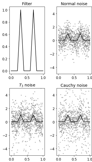
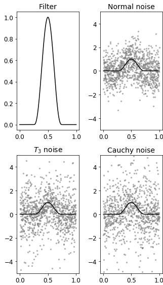
In our experiments, we considered three noise distributions: Gaussian distribution, Student t-distribution with 3 degrees of freedom, and Cauchy distribution. We took θ=0superscript𝜃0\theta^{*}=0 throughout, which is really without loss of generality since the two methods we compared — the standard method based on maximizing the Pearson correlation and the rank-based method that we study — are translation equivariant. We chose to work with the following three filters:

Template Af(x)={4x10.25x<0.5,34x0.5x<0.75,0otherwise,Template A𝑓𝑥cases4𝑥10.25𝑥0.534𝑥0.5𝑥0.750otherwise,\text{Template $A$: }\;\;f(x)=\begin{cases}4x-1&0.25\leq x<0.5,\\ 3-4x&0.5\leq x<0.75,\\ 0&\text{otherwise,}\end{cases} (7)
Template Bf(x)={10x20.2x<0.3,410x0.3x<0.4,10x60.6x<0.7,810x0.7x<0.8,0otherwiseTemplate B𝑓𝑥cases10𝑥20.2𝑥0.3410𝑥0.3𝑥0.410𝑥60.6𝑥0.7810𝑥0.7𝑥0.80otherwise\text{Template $B$: }\;\;f(x)=\begin{cases}10x-2&0.2\leq x<0.3,\\ 4-10x&0.3\leq x<0.4,\\ 10x-6&0.6\leq x<0.7,\\ 8-10x&0.7\leq x<0.8,\\ 0&\text{otherwise}\end{cases} (8)

and

Template Cf(x)=max{0,(1(4x2)2)3}.Template C𝑓𝑥0superscript1superscript4𝑥223\text{Template $C$: }\;\;f(x)=\max\{0,(1-(4x-2)^{2})^{3}\}. (9)

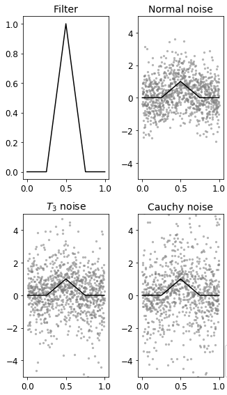
All are Lipschitz, with Template C𝐶C being even smoother. See Figure 1 for an illustration.
Refer to caption
(a) Template A𝐴A
Refer to caption
(b) Template B𝐵B
Refer to caption
(c) Template C𝐶C
Figure 1: Templates and noisy signals. Although the sample size is n=10000𝑛10000n=10000, for the sake of clarity, we only include 100010001000 points and limit the range of the y-axis to [5,5]55[-5,5].

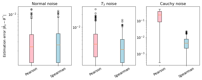
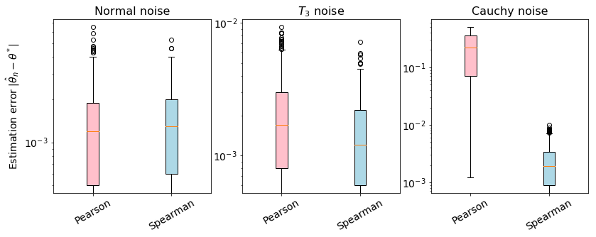
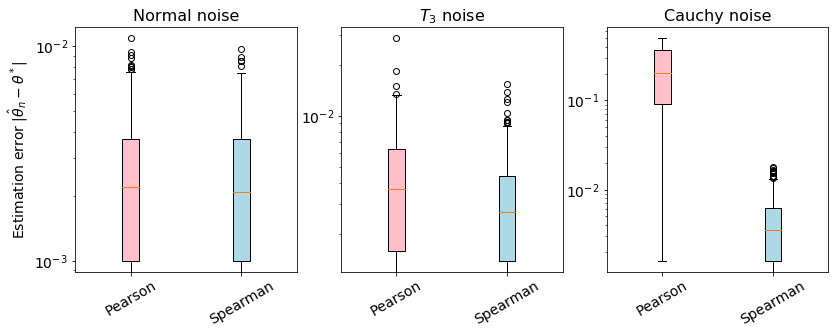
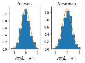
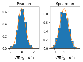
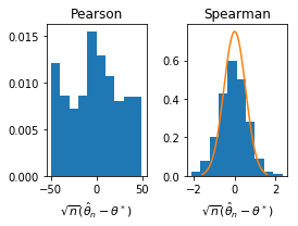
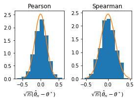
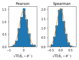
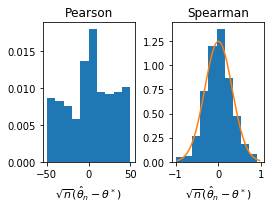
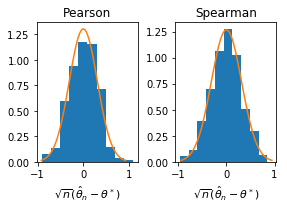
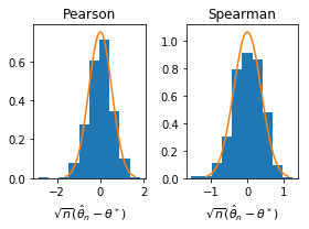
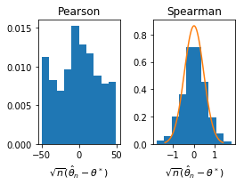
We set the sample size at n=10000𝑛10000n=10000. Each setting, defined by a choice of filter and of noise distribution, was repeated 500500500 times. Box plots of estimation error |θ^nθ|subscript^𝜃𝑛superscript𝜃|\hat{\theta}_{n}-\theta^{*}| are presented in Figures 2, 3 and 4, while the distribution of n(θ^nθ)𝑛subscript^𝜃𝑛superscript𝜃\sqrt{n}(\hat{\theta}_{n}-\theta^{*}) is depicted in Figures 5, 6 and 7 via histograms. The results are congruent with what the theory predicts: The rank-based method is slightly inferior to the standard method when the noise is Gaussian (exactly when the standard method coincides with the MLE), while it is superior when the noise distribution has heavier tails; and the histograms overlay nicely with the predicted asymptotic distribution. The asymptotic relative efficiency of R-estimator relative to the method based on maximizing the Pearson correlation is displayed in Table 1.

Template Noise
Normal Student t3subscript𝑡3t_{3} Cauchy
Template A𝐴A 0.949 2.008 \infty
Template B𝐵B 0.940 1.992 \infty
Template C𝐶C 0.948 2.008 \infty
Table 1: Asymptotic relative efficiency of the R-estimator (4) to the more common estimator (2). Note that the latter is asymptotically best in the setting of Gaussian noise as it then coincides with the maximum likelihood estimator for a ‘smooth’ model.
Refer to caption
Figure 2: Box plot of estimation error |θ^nθ|subscript^𝜃𝑛superscript𝜃|\hat{\theta}_{n}-\theta^{*}| for Template A𝐴A
Refer to caption
Figure 3: Box plot of estimation error |θ^nθ|subscript^𝜃𝑛superscript𝜃|\hat{\theta}_{n}-\theta^{*}| for Template B𝐵B
Refer to caption
Figure 4: Box plot of estimation error |θ^nθ|subscript^𝜃𝑛superscript𝜃|\hat{\theta}_{n}-\theta^{*}| for Template C𝐶C
Refer to caption
(a) Normal noise
Refer to caption
(b) T3subscript𝑇3T_{3} noise
Refer to caption
(c) Cauchy noise
Figure 5: Distribution under Template A𝐴A. The histogram presents the distribution of n(θ^nθ)𝑛subscript^𝜃𝑛superscript𝜃\sqrt{n}(\hat{\theta}_{n}-\theta^{*}). The orange bell-shaped curve is the density of normal distribution predicted by the theory.
Refer to caption
(a) Normal noise
Refer to caption
(b) T3subscript𝑇3T_{3} noise
Refer to caption
(c) Cauchy noise
Figure 6: Distribution under Template B𝐵B. The histogram presents the distribution of n(θ^nθ)𝑛subscript^𝜃𝑛superscript𝜃\sqrt{n}(\hat{\theta}_{n}-\theta^{*}). The orange bell-shaped curve is the density of normal distribution predicted by the theory.
Refer to caption
(a) Normal noise
Refer to caption
(b) T3subscript𝑇3T_{3} noise
Refer to caption
(c) Cauchy noise
Figure 7: Distribution under Template C𝐶C. The histogram presents the distribution of n(θ^nθ)𝑛subscript^𝜃𝑛superscript𝜃\sqrt{n}(\hat{\theta}_{n}-\theta^{*}). The orange bell-shaped curve is the density of normal distribution predicted by the theory.

4 Discussion

Our main goal in this paper was to show that a standard rank-based approach to template matching is viable and amenable to study using well-established techniques in mathematical statistics — some basic results in empirical process theory and the projection method of Hájek. This provides some theoretical foundation for related approaches proposed in recent years in the signal processing literature. We chose to keep the exposition contained and, in particular, have focused on the ‘smooth setting’ of a Lipschitz template. We leave the equally important case of a discontinuous template for future work (likely by others). Based on our previous work (Arias-Castro and Zheng, 2020) — where we did study this case in detail — and on our work here — in particular Hájek’s projection technique used in the proof of Theorem 2.6 — we do believe that the study of this case is within the reach of similarly standard tools.

Some of the other extensions discussed in our previous work are also relevant here. In particular, while we focused on shifts in the context of 1D signals, other settings are possible, including shifts in 2D or 3D signals (i.e., images), as well as other transformations. We omit details and simply affirm that such extensions are also amenable to a similar mathematical analysis.

In signal processing, rank-based methods seem more prominently represented in the literature on signal registration. We are confident that the study of such methods is well within the range of established techniques in mathematical statistics. However, the situation becomes substantially more complex as 1) the setting is semi-parametric, and 2) some smoothing seems to be required to achieve good performance — as transpires from the statistics literature on the topic as mentioned in our previous work (Arias-Castro and Zheng, 2020). We leave a further exploration of rank-based methods for registration to future endeavors.

5 Proofs

5.1 Preliminaries

The following is an extension of the celebrated Glivenko–Cantelli theorem.

Lemma 5.1.

Suppose that {Yi,n:i[n],n1}conditional-setsubscript𝑌𝑖𝑛formulae-sequence𝑖delimited-[]𝑛𝑛1\{Y_{i,n}:i\in[n],n\geq 1\} are independent random variables with uniformly tight and equicontinuous distributions {Fi,n:i[n],n1}conditional-setsubscript𝐹𝑖𝑛formulae-sequence𝑖delimited-[]𝑛𝑛1\{F_{i,n}:i\in[n],n\geq 1\}. Define

F^[n](y):=1ni=1n𝕀{Yi,ny},assignsubscript^𝐹delimited-[]𝑛𝑦1𝑛superscriptsubscript𝑖1𝑛𝕀subscript𝑌𝑖𝑛𝑦\displaystyle\hat{F}_{[n]}(y):=\frac{1}{n}\sum_{i=1}^{n}\mathbb{I}{\{Y_{i,n}\leq y\}}, F[n]:=𝔼[F^[n]]=1ni=1nFi,n.assignsubscript𝐹delimited-[]𝑛𝔼subscript^𝐹delimited-[]𝑛1𝑛superscriptsubscript𝑖1𝑛subscript𝐹𝑖𝑛\displaystyle F_{[n]}:=\operatorname{\mathbb{E}}[\hat{F}_{[n]}]=\frac{1}{n}\sum_{i=1}^{n}F_{i,n}.

Then the following uniform convergence holds in probability

supt|F^[n](t)F[n](t)|n0.𝑛subscriptsupremum𝑡subscript^𝐹delimited-[]𝑛𝑡subscript𝐹delimited-[]𝑛𝑡0\displaystyle\sup_{t}|\hat{F}_{[n]}(t)-F_{[n]}(t)|\xrightarrow{n\to\infty}0.
Proof.

The proof arguments are very close to those supporting the more classical situation in which the random variables have the same distribution (Van der Vaart, 1998, Th 19.1). We provide a proof for completeness only.

Our assumptions mean 1) that for each ε>0𝜀0\varepsilon>0 there is K𝐾K such that infiFi,n(K)1εsubscriptinfimum𝑖subscript𝐹𝑖𝑛𝐾1𝜀\inf_{i}F_{i,n}(K)\geq 1-\varepsilon and supiFi,n(K)εsubscriptsupremum𝑖subscript𝐹𝑖𝑛𝐾𝜀\sup_{i}F_{i,n}(-K)\leq\varepsilon; and 2) that ω(δ):=supisupt(Fi,n(t+δ)Fi,n(t))assign𝜔𝛿subscriptsupremum𝑖subscriptsupremum𝑡subscript𝐹𝑖𝑛𝑡𝛿subscript𝐹𝑖𝑛𝑡\omega(\delta):=\sup_{i}\sup_{t}(F_{i,n}(t+\delta)-F_{i,n}(t)) is continuous at 0; we then speak of ω𝜔\omega as the modulus of continuity of the family {Fi,n}subscript𝐹𝑖𝑛\{F_{i,n}\}. Fix ε>0𝜀0\varepsilon>0 and let K𝐾K be defined as above. Also, let δ𝛿\delta be such that ω(δ)ε𝜔𝛿𝜀\omega(\delta)\leq\varepsilon and set K=t1<t2<<tm1<tm=K𝐾subscript𝑡1subscript𝑡2subscript𝑡𝑚1subscript𝑡𝑚𝐾-K=t_{1}<t_{2}<\dots<t_{m-1}<t_{m}=K be such that tj+1tjδsubscript𝑡𝑗1subscript𝑡𝑗𝛿t_{j+1}-t_{j}\leq\delta for all j𝑗j. We then have, regardless of n𝑛n, that F[n](K)1εsubscript𝐹delimited-[]𝑛𝐾1𝜀F_{[n]}(K)\geq 1-\varepsilon and F[n](K)εsubscript𝐹delimited-[]𝑛𝐾𝜀F_{[n]}(-K)\leq\varepsilon; and that ω𝜔\omega is a modulus of continuity for F[n]subscript𝐹delimited-[]𝑛F_{[n]}, meaning that supt(F[n](t+δ)F[n](t))ω(δ)subscriptsupremum𝑡subscript𝐹delimited-[]𝑛𝑡𝛿subscript𝐹delimited-[]𝑛𝑡𝜔𝛿\sup_{t}(F_{[n]}(t+\delta)-F_{[n]}(t))\leq\omega(\delta).

  • For tt1𝑡subscript𝑡1t\leq t_{1}, we have

    |F^[n](t)F[n](t)|F^[n](t)+F[n](t)F^[n](t1)+ε.subscript^𝐹delimited-[]𝑛𝑡subscript𝐹delimited-[]𝑛𝑡subscript^𝐹delimited-[]𝑛𝑡subscript𝐹delimited-[]𝑛𝑡subscript^𝐹delimited-[]𝑛subscript𝑡1𝜀\displaystyle|\hat{F}_{[n]}(t)-F_{[n]}(t)|\leq\hat{F}_{[n]}(t)+F_{[n]}(t)\leq\hat{F}_{[n]}(t_{1})+\varepsilon.
  • For ttm𝑡subscript𝑡𝑚t\geq t_{m}, we have

    |F^[n](t)F[n](t)|(1F^[n](t))+(1F[n](t))(1F^[n](tm))+ε.subscript^𝐹delimited-[]𝑛𝑡subscript𝐹delimited-[]𝑛𝑡1subscript^𝐹delimited-[]𝑛𝑡1subscript𝐹delimited-[]𝑛𝑡1subscript^𝐹delimited-[]𝑛subscript𝑡𝑚𝜀\displaystyle|\hat{F}_{[n]}(t)-F_{[n]}(t)|\leq(1-\hat{F}_{[n]}(t))+(1-F_{[n]}(t))\leq(1-\hat{F}_{[n]}(t_{m}))+\varepsilon.
  • For K<t<K𝐾𝑡𝐾-K<t<K, if j𝑗j is such that tj<ttj+1subscript𝑡𝑗𝑡subscript𝑡𝑗1t_{j}<t\leq t_{j+1},

    F^[n](t)F[n](t)F^[n](tj+1)F[n](tj)F^[n](tj+1)F[n](tj+1)+ε,subscript^𝐹delimited-[]𝑛𝑡subscript𝐹delimited-[]𝑛𝑡subscript^𝐹delimited-[]𝑛subscript𝑡𝑗1subscript𝐹delimited-[]𝑛subscript𝑡𝑗subscript^𝐹delimited-[]𝑛subscript𝑡𝑗1subscript𝐹delimited-[]𝑛subscript𝑡𝑗1𝜀\displaystyle\hat{F}_{[n]}(t)-F_{[n]}(t)\leq\hat{F}_{[n]}(t_{j+1})-F_{[n]}(t_{j})\leq\hat{F}_{[n]}(t_{j+1})-F_{[n]}(t_{j+1})+\varepsilon,

    and

    F^[n](t)F[n](t)F^[n](tj)F[n](tj+1)F^[n](tj)F[n](tj)ε.subscript^𝐹delimited-[]𝑛𝑡subscript𝐹delimited-[]𝑛𝑡subscript^𝐹delimited-[]𝑛subscript𝑡𝑗subscript𝐹delimited-[]𝑛subscript𝑡𝑗1subscript^𝐹delimited-[]𝑛subscript𝑡𝑗subscript𝐹delimited-[]𝑛subscript𝑡𝑗𝜀\displaystyle\hat{F}_{[n]}(t)-F_{[n]}(t)\geq\hat{F}_{[n]}(t_{j})-F_{[n]}(t_{j+1})\leq\hat{F}_{[n]}(t_{j})-F_{[n]}(t_{j})-\varepsilon.

By Chebyshev’s inequality, F^[n](t)F[n](t)0subscript^𝐹delimited-[]𝑛𝑡subscript𝐹delimited-[]𝑛𝑡0\hat{F}_{[n]}(t)-F_{[n]}(t)\to 0 in probability as n𝑛n\to\infty for every fixed t𝑡t\in\mathbb{R}. In particular, maxj|F^[n](tj)F[n](tj)|0subscript𝑗subscript^𝐹delimited-[]𝑛subscript𝑡𝑗subscript𝐹delimited-[]𝑛subscript𝑡𝑗0\max_{j}|\hat{F}_{[n]}(t_{j})-F_{[n]}(t_{j})|\to 0 in probability, and under the event that this maximum is bounded by ε𝜀\varepsilon, we have |F^[n](t)F[n](t)|2εsubscript^𝐹delimited-[]𝑛𝑡subscript𝐹delimited-[]𝑛𝑡2𝜀|\hat{F}_{[n]}(t)-F_{[n]}(t)|\leq 2\varepsilon. Since ε>0𝜀0\varepsilon>0 is arbitrary, the proof is complete. ∎

The following is a simple result on functions defined as the linear combination of uniformly equicontinuous functions with random coefficients.

Lemma 5.2.

Suppose that {Bi,n:i[n],n1}conditional-setsubscript𝐵𝑖𝑛formulae-sequence𝑖delimited-[]𝑛𝑛1\{B_{i,n}:i\in[n],n\geq 1\} are independent such that |Bi,n|Ksubscript𝐵𝑖𝑛𝐾|B_{i,n}|\leq K and 𝔼[Bi,n]=0𝔼subscript𝐵𝑖𝑛0\operatorname{\mathbb{E}}[B_{i,n}]=0 for all i[n]𝑖delimited-[]𝑛i\in[n] and all n1𝑛1n\geq 1; and that {fi,n:i[n],n1}conditional-setsubscript𝑓𝑖𝑛formulae-sequence𝑖delimited-[]𝑛𝑛1\{f_{i,n}:i\in[n],n\geq 1\} are uniformly bounded and uniformly equicontinuous functions either defined on a compact interval. Then, in probability,

|1ni=1nBi,nfi,n|n0.𝑛subscript1𝑛superscriptsubscript𝑖1𝑛subscript𝐵𝑖𝑛subscript𝑓𝑖𝑛0\displaystyle\Big{|}\frac{1}{n}\sum_{i=1}^{n}B_{i,n}f_{i,n}\Big{|}_{\infty}\xrightarrow{n\to\infty}0.
Proof.

The arguments are quite similar to those supporting Lemma 5.1. Define

Sn:=1ni=1nBi,nfi,n.assignsubscript𝑆𝑛1𝑛superscriptsubscript𝑖1𝑛subscript𝐵𝑖𝑛subscript𝑓𝑖𝑛\displaystyle S_{n}:=\frac{1}{n}\sum_{i=1}^{n}B_{i,n}f_{i,n}.

Suppose without loss of generality that the functions are defined on the unit interval. Because they are uniformly equicontinuous, for any given ε>0𝜀0\varepsilon>0, there is δ>0𝛿0\delta>0 such that supnsupi|fi,n(t)fi,n(s)|εsubscriptsupremum𝑛subscriptsupremum𝑖subscript𝑓𝑖𝑛𝑡subscript𝑓𝑖𝑛𝑠𝜀\sup_{n}\sup_{i}|f_{i,n}(t)-f_{i,n}(s)|\leq\varepsilon for all s,t[0,1]𝑠𝑡01s,t\in[0,1] such that |ts|δ𝑡𝑠𝛿|t-s|\leq\delta. With ε>0𝜀0\varepsilon>0 fixed, and δ𝛿\delta as such, let 0=t1<t2<<tm1<tm=10subscript𝑡1subscript𝑡2subscript𝑡𝑚1subscript𝑡𝑚10=t_{1}<t_{2}<\cdots<t_{m-1}<t_{m}=1 be such that tj+1tjδsubscript𝑡𝑗1subscript𝑡𝑗𝛿t_{j+1}-t_{j}\leq\delta for all j𝑗j. Then for any t[0,1]𝑡01t\in[0,1], if j𝑗j is such that tjttj+1subscript𝑡𝑗𝑡subscript𝑡𝑗1t_{j}\leq t\leq t_{j+1},

|Sn(t)Sn(tj)|1ni=1n|Bi,n||fi,n(t)fi,n(tj)|Ksupnsupi|fi,n(t)fi,n(tj)|Kε.subscript𝑆𝑛𝑡subscript𝑆𝑛subscript𝑡𝑗1𝑛superscriptsubscript𝑖1𝑛subscript𝐵𝑖𝑛subscript𝑓𝑖𝑛𝑡subscript𝑓𝑖𝑛subscript𝑡𝑗𝐾subscriptsupremum𝑛subscriptsupremum𝑖subscript𝑓𝑖𝑛𝑡subscript𝑓𝑖𝑛subscript𝑡𝑗𝐾𝜀\displaystyle|S_{n}(t)-S_{n}(t_{j})|\leq\frac{1}{n}\sum_{i=1}^{n}|B_{i,n}||f_{i,n}(t)-f_{i,n}(t_{j})|\leq K\sup_{n}\sup_{i}|f_{i,n}(t)-f_{i,n}(t_{j})|\leq K\varepsilon.

In particular,

|Sn|maxj|Sn(tj)|+Kε.subscriptsubscript𝑆𝑛subscript𝑗subscript𝑆𝑛subscript𝑡𝑗𝐾𝜀\displaystyle|S_{n}|_{\infty}\leq\max_{j}|S_{n}(t_{j})|+K\varepsilon.

Furthermore, by Chebyshev’s inequality, in probability,

maxj|Sn(tj)|n0.𝑛subscript𝑗subscript𝑆𝑛subscript𝑡𝑗0\displaystyle\max_{j}|S_{n}(t_{j})|\xrightarrow{n\to\infty}0.

Hence, in probability,

lim supn|Sn|Kε.subscriptlimit-supremum𝑛subscriptsubscript𝑆𝑛𝐾𝜀\displaystyle\limsup_{n}|S_{n}|_{\infty}\leq K\varepsilon.

Since ε>0𝜀0\varepsilon>0 was chosen arbitrary, the proof is complete. ∎

The following is a well-known error bound for Riemann sums.

Lemma 5.3.

Assume that f:[a,b]:𝑓𝑎𝑏f:[a,b]\to\mathbb{R} is continuous with modulus of continuity ω𝜔\omega. Then

|abf(u)du1mj=1mf(a+j(ba)/m)|superscriptsubscript𝑎𝑏𝑓𝑢differential-d𝑢1𝑚superscriptsubscript𝑗1𝑚𝑓𝑎𝑗𝑏𝑎𝑚\displaystyle\left|\int_{a}^{b}f(u){\rm d}u-\frac{1}{m}\sum_{j=1}^{m}f(a+j(b-a)/m)\right| (ba)ω((ba)/m)absent𝑏𝑎𝜔𝑏𝑎𝑚\displaystyle\leq(b-a)\omega((b-a)/m)
(ba)2m|f|if f is Lipschitz.absentsuperscript𝑏𝑎2𝑚subscriptsuperscript𝑓if f is Lipschitz.\displaystyle\leq\frac{(b-a)^{2}}{m}\,|f^{\prime}|_{\infty}\quad\text{if $f$ is Lipschitz.}
Proof.

This well-known result is a simple consequence of partitioning [a,b]𝑎𝑏[a,b] into sub-intervals of length (ba)/m𝑏𝑎𝑚(b-a)/m. ∎

The next two lemmas are refinements of Lemma 5.1 and Lemma 5.2. They clearly subsume them, but they are also much deeper, and we only provide proof sketches, relying on arguments borrowed from (Van der Vaart, 1998).

Lemma 5.4.

In the context of Lemma 5.1, for some constant C𝐶C,

𝔼[supt|F^[n](t)F[n](t)|]C/n.𝔼subscriptsupremum𝑡subscript^𝐹delimited-[]𝑛𝑡subscript𝐹delimited-[]𝑛𝑡𝐶𝑛\displaystyle\operatorname{\mathbb{E}}\Big{[}\sup_{t}|\hat{F}_{[n]}(t)-F_{[n]}(t)|\Big{]}\leq C/\sqrt{n}.
Proof.

The result is classical when the variables are not only independent, but also identically distributed, say Yi,nFsimilar-tosubscript𝑌𝑖𝑛𝐹Y_{i,n}\sim F for all i𝑖i and all n𝑛n, and is a special case of so-called entropy bounds on the supremum of an empirical processes of the form

Sn:=supg𝒢1ni=1n(g(Yi,n)𝔼[g(Yi,n)]).assignsubscript𝑆𝑛subscriptsupremum𝑔𝒢1𝑛superscriptsubscript𝑖1𝑛𝑔subscript𝑌𝑖𝑛𝔼𝑔subscript𝑌𝑖𝑛S_{n}:=\sup_{g\in\mathcal{G}}\frac{1}{\sqrt{n}}\sum_{i=1}^{n}(g(Y_{i,n})-\operatorname{\mathbb{E}}[g(Y_{i,n})]). (10)

For example, assuming that the class 𝒢𝒢\mathcal{G} is uniformly bounded, Cor 19.35 in (Van der Vaart, 1998) gives

𝔼[Sn]C0J(𝒢,F),𝔼subscript𝑆𝑛subscript𝐶0𝐽𝒢𝐹\operatorname{\mathbb{E}}[S_{n}]\leq C_{0}J(\mathcal{G},F),

where C0subscript𝐶0C_{0} is a constant and

J(𝒢,F):=0logN(ε,𝒢,L2(F))dε,assign𝐽𝒢𝐹superscriptsubscript0𝑁𝜀𝒢superscript𝐿2𝐹differential-d𝜀J(\mathcal{G},F):=\int_{0}^{\infty}\sqrt{\log N(\varepsilon,\mathcal{G},L^{2}(F))}{\rm d}\varepsilon,

N(ε,𝒢,L2(F))𝑁𝜀𝒢superscript𝐿2𝐹N(\varepsilon,\mathcal{G},L^{2}(F)) denoting the ε𝜀\varepsilon-bracketing number of the class 𝒢𝒢\mathcal{G} with respect to the L2(F)superscript𝐿2𝐹L^{2}(F) metric.111Two functions g1,g2subscript𝑔1subscript𝑔2g_{1},g_{2} such that g1g2subscript𝑔1subscript𝑔2g_{1}\leq g_{2} pointwise define a bracket made of all functions g𝑔g such that g1gg2subscript𝑔1𝑔subscript𝑔2g_{1}\leq g\leq g_{2}. It is said to be an ε𝜀\varepsilon-bracket with respect to L2(F)superscript𝐿2𝐹L^{2}(F), for a positive measure F𝐹F, if (g2g1)2dFε2superscriptsubscript𝑔2subscript𝑔12differential-d𝐹superscript𝜀2\int(g_{2}-g_{1})^{2}{\rm d}F\leq\varepsilon^{2}. Given a class of functions 𝒢𝒢\mathcal{G}, its ε𝜀\varepsilon-bracketing number with respect to L2(F)superscript𝐿2𝐹L^{2}(F) is the minimum number of ε𝜀\varepsilon-brackets needed to cover 𝒢𝒢\mathcal{G}.

The proof of that result takes several pages, but a close examination reveals that the ‘identically distributed’ property is not used in an essential way. Indeed, the assumption that the variables are iid is only used when applying Bernstein’s concentration inequality (Lem 19.32 there), and it is well-known that the result applies in a generalized form to variables that are only independent, say Yi,nFi,nsimilar-tosubscript𝑌𝑖𝑛subscript𝐹𝑖𝑛Y_{i,n}\sim F_{i,n}. Everything follows from that, essentially verbatim, and yields

𝔼[Sn]C0J(𝒢,F[n]).𝔼subscript𝑆𝑛subscript𝐶0𝐽𝒢subscript𝐹delimited-[]𝑛\operatorname{\mathbb{E}}[S_{n}]\leq C_{0}J(\mathcal{G},F_{[n]}).

It turns out that, for a given distribution function F𝐹F, J(𝒢,F)𝐽𝒢𝐹J(\mathcal{G},F) can be bounded based on the modulus of continuity of F𝐹F (see Ex 19.6 in the same reference). And if ω𝜔\omega is the modulus of continuity of {Fi,n}subscript𝐹𝑖𝑛\{F_{i,n}\}, then it is also a modulus of continuity for F[n]subscript𝐹delimited-[]𝑛F_{[n]}, and with this we can bound J(𝒢,F[n])𝐽𝒢subscript𝐹delimited-[]𝑛J(\mathcal{G},F_{[n]}) independently of n𝑛n just based on ω𝜔\omega.

When dealing with the empirical distribution function, which is our focus here, the class is taken to be 𝒢:={𝕀{yt}:t}assign𝒢conditional-set𝕀𝑦𝑡𝑡\mathcal{G}:=\{\mathbb{I}{\{y\leq t\}}:t\in\mathbb{R}\}. For that class, J(𝒢,F)<𝐽𝒢𝐹J(\mathcal{G},F)<\infty for any distribution function, and this implies via the arguments above that supnJ(𝒢,F[n])<subscriptsupremum𝑛𝐽𝒢subscript𝐹delimited-[]𝑛\sup_{n}J(\mathcal{G},F_{[n]})<\infty, concluding the proof. ∎

Lemma 5.5.

Suppose that {Bi:i1}conditional-setsubscript𝐵𝑖𝑖1\{B_{i}:i\geq 1\} are independent random variables that are centered and bounded in absolute value by K𝐾K. And let {fi:i1}conditional-setsubscript𝑓𝑖𝑖1\{f_{i}:i\geq 1\} be L𝐿L-Lipschitz functions on [t0,t0]subscript𝑡0subscript𝑡0[-t_{0},t_{0}] with fi(0)=0subscript𝑓𝑖00f_{i}(0)=0 for all i𝑖i. Then there is a some constant C𝐶C such that, for any n1𝑛1n\geq 1,

𝔼[sup|t|t0|1ni=1nBifi(t)|]Ct0n.𝔼subscriptsupremum𝑡subscript𝑡01𝑛superscriptsubscript𝑖1𝑛subscript𝐵𝑖subscript𝑓𝑖𝑡𝐶subscript𝑡0𝑛\displaystyle\operatorname{\mathbb{E}}\bigg{[}\sup_{|t|\leq t_{0}}\Big{|}\frac{1}{n}\sum_{i=1}^{n}B_{i}f_{i}(t)\Big{|}\bigg{]}\leq\frac{Ct_{0}}{\sqrt{n}}.
Proof.

As in the proof of Lemma 5.4, we rely on entropy bounds. Here we use Dudley’s entropy bound as presented in (Giné and Nickl, 2016, Th 2.3.6). For a given n𝑛n, let S(t):=1ni=1nBifi(t)assign𝑆𝑡1𝑛superscriptsubscript𝑖1𝑛subscript𝐵𝑖subscript𝑓𝑖𝑡S(t):=\frac{1}{n}\sum_{i=1}^{n}B_{i}f_{i}(t), we have

S(t)S(s)=i=1nBin(fi(t)fi(s)),𝑆𝑡𝑆𝑠superscriptsubscript𝑖1𝑛subscript𝐵𝑖𝑛subscript𝑓𝑖𝑡subscript𝑓𝑖𝑠S(t)-S(s)=\sum_{i=1}^{n}\frac{B_{i}}{n}(f_{i}(t)-f_{i}(s)), (11)

with the variables Bin(fi(t)fi(s))subscript𝐵𝑖𝑛subscript𝑓𝑖𝑡subscript𝑓𝑖𝑠\frac{B_{i}}{n}(f_{i}(t)-f_{i}(s)) being independent, centered, and bounded in absolute value by (K/n)L|ts|𝐾𝑛𝐿𝑡𝑠(K/n)L|t-s|. In (Giné and Nickl, 2016), by Eq (3.8) and based on Def 2.3.5, the process S(t)𝑆𝑡S(t) is sub-Gaussian on [t0,t0]subscript𝑡0subscript𝑡0[-t_{0},t_{0}] with respect to the metric d(s,t):=(KL/n)|st|assignd𝑠𝑡𝐾𝐿𝑛𝑠𝑡{\rm d}(s,t):=(KL/\sqrt{n})|s-t|. Because S(0)=0𝑆00S(0)=0, Th 2.3.6 there gives that

𝔼[sup|t|t0|S(t)|]420D/2log(2N(ε))dε,𝔼subscriptsupremum𝑡subscript𝑡0𝑆𝑡42superscriptsubscript0𝐷22𝑁𝜀differential-d𝜀\displaystyle\operatorname{\mathbb{E}}\Big{[}\sup_{|t|\leq t_{0}}|S(t)|\Big{]}\leq 4\sqrt{2}\int_{0}^{D/2}\sqrt{\log(2N(\varepsilon))}{\rm d}\varepsilon,

where D𝐷D and N(ε)𝑁𝜀N(\varepsilon) are the diameter and ε𝜀\varepsilon-covering number of [t0,t0]subscript𝑡0subscript𝑡0[-t_{0},t_{0}] with respect to dd{\rm d}. Immediately, D=(KL/n)(2t0)=2KLt0/n𝐷𝐾𝐿𝑛2subscript𝑡02𝐾𝐿subscript𝑡0𝑛D=(KL/\sqrt{n})(2t_{0})=2KLt_{0}/\sqrt{n}, and N(ε)(KL/n)(t0/ε)D/εasymptotically-equals𝑁𝜀𝐾𝐿𝑛subscript𝑡0𝜀asymptotically-equals𝐷𝜀N(\varepsilon)\asymp(KL/\sqrt{n})(t_{0}/\varepsilon)\asymp D/\varepsilon. With a simple change of variable in the integral, this gives us

𝔼[sup|t|t0|S(t)|]C1KLt0/n,𝔼subscriptsupremum𝑡subscript𝑡0𝑆𝑡subscript𝐶1𝐾𝐿subscript𝑡0𝑛\displaystyle\operatorname{\mathbb{E}}\Big{[}\sup_{|t|\leq t_{0}}|S(t)|\Big{]}\leq C_{1}KLt_{0}/\sqrt{n},

for a universal constant C1subscript𝐶1C_{1}. ∎

5.2 Proof of Lemma 2.1

We assume without loss of generality that θ=0superscript𝜃0\theta^{*}=0. We have

Ri=j=1n𝕀{YjYi}=nΨ^n(Yi),where Ψ^n(y):=1nj=1n𝕀{Yjy}.formulae-sequencesubscript𝑅𝑖superscriptsubscript𝑗1𝑛𝕀subscript𝑌𝑗subscript𝑌𝑖𝑛subscript^Ψ𝑛subscript𝑌𝑖assignwhere subscript^Ψ𝑛𝑦1𝑛superscriptsubscript𝑗1𝑛𝕀subscript𝑌𝑗𝑦\displaystyle R_{i}=\sum_{j=1}^{n}\mathbb{I}{\{Y_{j}\leq Y_{i}\}}=n\hat{\Psi}_{n}(Y_{i}),\quad\text{where }\hat{\Psi}_{n}(y):=\frac{1}{n}\sum_{j=1}^{n}\mathbb{I}{\{Y_{j}\leq y\}}.

Note that Ψ^nsubscript^Ψ𝑛\hat{\Psi}_{n} is the empirical distribution function of Y1,,Ynsubscript𝑌1subscript𝑌𝑛Y_{1},\dots,Y_{n}. Although these are not iid, they are independent, and the Glivenko–Cantelli theorem applies to give that, in probability,

supy|Ψ^n(y)𝔼[Ψ^n(y)]|n0.𝑛subscriptsupremum𝑦subscript^Ψ𝑛𝑦𝔼subscript^Ψ𝑛𝑦0\displaystyle\sup_{y\in\mathbb{R}}|\hat{\Psi}_{n}(y)-\operatorname{\mathbb{E}}[\hat{\Psi}_{n}(y)]|\xrightarrow{n\to\infty}0.

See Lemma 5.1 for details. Further, we have

𝔼[Ψ^n(y)]𝔼subscript^Ψ𝑛𝑦\displaystyle\operatorname{\mathbb{E}}[\hat{\Psi}_{n}(y)] =1nj=1n(Yjy)absent1𝑛superscriptsubscript𝑗1𝑛subscript𝑌𝑗𝑦\displaystyle=\frac{1}{n}\sum_{j=1}^{n}\operatorname{\mathbb{P}}(Y_{j}\leq y)
=1nj=1n(Zjyf(xj))absent1𝑛superscriptsubscript𝑗1𝑛subscript𝑍𝑗𝑦𝑓subscript𝑥𝑗\displaystyle=\frac{1}{n}\sum_{j=1}^{n}\operatorname{\mathbb{P}}(Z_{j}\leq y-f(x_{j}))
=1nj=1nΦ(yf(j/n))absent1𝑛superscriptsubscript𝑗1𝑛Φ𝑦𝑓𝑗𝑛\displaystyle=\frac{1}{n}\sum_{j=1}^{n}\Phi(y-f(j/n))
nΨ(y):=01Φ(yf(x))dx,𝑛absentΨ𝑦assignsuperscriptsubscript01Φ𝑦𝑓𝑥differential-d𝑥\displaystyle\xrightarrow{n\to\infty}\Psi(y):=\int_{0}^{1}\Phi(y-f(x)){\rm d}x,

where the convergence is by definition of the Riemann integral defining the limit. The convergence is in fact uniform in y𝑦y. This comes from an application of Lemma 5.3 using with the fact that xΦ(yf(x))maps-to𝑥Φ𝑦𝑓𝑥x\mapsto\Phi(y-f(x)) has derivative f(x)ϕ(yf(x))superscript𝑓𝑥italic-ϕ𝑦𝑓𝑥f^{\prime}(x)\phi(y-f(x)), which has supremum norm bounded by |f||ϕ|<subscriptsuperscript𝑓subscriptitalic-ϕ|f^{\prime}|_{\infty}|\phi|_{\infty}<\infty (independent of y𝑦y). Hence, a simple application of the triangle inequality gives that, in probability,

A1,n:=supy|Ψ^n(y)Ψ(y)|n0.assignsubscript𝐴1𝑛subscriptsupremum𝑦subscript^Ψ𝑛𝑦Ψ𝑦𝑛0\displaystyle A_{1,n}:=\sup_{y\in\mathbb{R}}|\hat{\Psi}_{n}(y)-\Psi(y)|\xrightarrow{n\to\infty}0. (12)

This is useful to us because Ri=nΨ(Yi)±nA1,nsubscript𝑅𝑖plus-or-minus𝑛Ψsubscript𝑌𝑖𝑛subscript𝐴1𝑛R_{i}=n\Psi(Y_{i})\pm nA_{1,n}, which then triggers

M^n(θ)=1ni=1nΨ(Yi)f(xiθ)±A2,n,subscript^𝑀𝑛𝜃plus-or-minus1𝑛superscriptsubscript𝑖1𝑛Ψsubscript𝑌𝑖𝑓subscript𝑥𝑖𝜃subscript𝐴2𝑛\displaystyle\widehat{M}_{n}(\theta)=\frac{1}{n}\sum_{i=1}^{n}\Psi(Y_{i})f(x_{i}-\theta)\pm A_{2,n},

with A2,n:=A1,n|f|=oP(1)assignsubscript𝐴2𝑛subscript𝐴1𝑛subscript𝑓subscript𝑜𝑃1A_{2,n}:=A_{1,n}|f|_{\infty}=o_{P}(1). We may thus focus on the first term on the right-hand side. We have

1ni=1nΨ(Yi)f(xiθ)=1ni=1n𝔼[Ψ(Yi)]f(xiθ)+Qn(θ),1𝑛superscriptsubscript𝑖1𝑛Ψsubscript𝑌𝑖𝑓subscript𝑥𝑖𝜃1𝑛superscriptsubscript𝑖1𝑛𝔼Ψsubscript𝑌𝑖𝑓subscript𝑥𝑖𝜃subscript𝑄𝑛𝜃\displaystyle\frac{1}{n}\sum_{i=1}^{n}\Psi(Y_{i})f(x_{i}-\theta)=\frac{1}{n}\sum_{i=1}^{n}\operatorname{\mathbb{E}}[\Psi(Y_{i})]f(x_{i}-\theta)+Q_{n}(\theta),

with

Qn(θ):=1ni=1n(Ψ(Yi)𝔼[Ψ(Yi)])f(xiθ).assignsubscript𝑄𝑛𝜃1𝑛superscriptsubscript𝑖1𝑛Ψsubscript𝑌𝑖𝔼Ψsubscript𝑌𝑖𝑓subscript𝑥𝑖𝜃\displaystyle Q_{n}(\theta):=\frac{1}{n}\sum_{i=1}^{n}(\Psi(Y_{i})-\operatorname{\mathbb{E}}[\Psi(Y_{i})])f(x_{i}-\theta).

On the one hand, by a standard argument consisting in discretizing the values of θ𝜃\theta and using the uniform continuity of f𝑓f, we obtain

A3,n:=supθ|Qn(θ)|n0,assignsubscript𝐴3𝑛subscriptsupremum𝜃subscript𝑄𝑛𝜃𝑛0\displaystyle A_{3,n}:=\sup_{\theta\in\mathbb{R}}|Q_{n}(\theta)|\xrightarrow{n\to\infty}0,

in probability. See Lemma 5.2 for details. On the other hand,

1ni=1n𝔼[Ψ(Yi)]f(xiθ)1𝑛superscriptsubscript𝑖1𝑛𝔼Ψsubscript𝑌𝑖𝑓subscript𝑥𝑖𝜃\displaystyle\frac{1}{n}\sum_{i=1}^{n}\operatorname{\mathbb{E}}[\Psi(Y_{i})]f(x_{i}-\theta) =1ni=1nΨ(z+f(i/n))ϕ(z)dzf(i/nθ)absent1𝑛superscriptsubscript𝑖1𝑛superscriptsubscriptΨ𝑧𝑓𝑖𝑛italic-ϕ𝑧differential-d𝑧𝑓𝑖𝑛𝜃\displaystyle=\frac{1}{n}\sum_{i=1}^{n}\int_{-\infty}^{\infty}\Psi(z+f(i/n))\phi(z){\rm d}z\cdot f(i/n-\theta)
n01Ψ(z+f(x))ϕ(z)dzf(xθ)dx𝑛absentsuperscriptsubscript01superscriptsubscriptΨ𝑧𝑓𝑥italic-ϕ𝑧differential-d𝑧𝑓𝑥𝜃differential-d𝑥\displaystyle\xrightarrow{n\to\infty}\int_{0}^{1}\int_{-\infty}^{\infty}\Psi(z+f(x))\phi(z){\rm d}z\cdot f(x-\theta){\rm d}x
=0101Φ2(f(x)f(t))f(xθ)dtdx=M(θ),absentsuperscriptsubscript01superscriptsubscript01subscriptΦ2𝑓𝑥𝑓𝑡𝑓𝑥𝜃differential-d𝑡differential-d𝑥𝑀𝜃\displaystyle\qquad\qquad=\int_{0}^{1}\int_{0}^{1}\Phi_{2}(f(x)-f(t))f(x-\theta){\rm d}t{\rm d}x=M(\theta),

using again the definition of Riemann integral. In fact the convergence is uniform in θ𝜃\theta, by an application of Lemma 5.3 to the function

gθ(x):=Ψ(z+f(x))ϕ(z)dzf(xθ),assignsubscript𝑔𝜃𝑥superscriptsubscriptΨ𝑧𝑓𝑥italic-ϕ𝑧differential-d𝑧𝑓𝑥𝜃g_{\theta}(x):=\int_{-\infty}^{\infty}\Psi(z+f(x))\phi(z){\rm d}z\cdot f(x-\theta),

whose derivative can be bounded independently of θ𝜃\theta as follows:

|gθ(x)|superscriptsubscript𝑔𝜃𝑥\displaystyle|g_{\theta}^{\prime}(x)| =|f(x)Ψ(z+f(x))ϕ(z)dzf(xθ)+Ψ(z+f(x))ϕ(z)dzf(xθ)|absentsuperscriptsubscriptsuperscript𝑓𝑥superscriptΨ𝑧𝑓𝑥italic-ϕ𝑧differential-d𝑧𝑓𝑥𝜃superscriptsubscriptΨ𝑧𝑓𝑥italic-ϕ𝑧differential-d𝑧superscript𝑓𝑥𝜃\displaystyle=\Big{|}\int_{-\infty}^{\infty}f^{\prime}(x)\Psi^{\prime}(z+f(x))\phi(z){\rm d}z\cdot f(x-\theta)+\int_{-\infty}^{\infty}\Psi(z+f(x))\phi(z){\rm d}z\cdot f^{\prime}(x-\theta)\Big{|}
|f||Ψ||f|+|Ψ||f|absentsubscriptsuperscript𝑓subscriptsuperscriptΨsubscript𝑓subscriptΨsubscriptsuperscript𝑓\displaystyle\leq|f^{\prime}|_{\infty}|\Psi^{\prime}|_{\infty}|f|_{\infty}+|\Psi|_{\infty}|f^{\prime}|_{\infty}
|f||ϕ||f|+|f|,absentsubscriptsuperscript𝑓subscriptitalic-ϕsubscript𝑓subscriptsuperscript𝑓\displaystyle\leq|f^{\prime}|_{\infty}|\phi|_{\infty}|f|_{\infty}+|f^{\prime}|_{\infty},

using the fact that ϕitalic-ϕ\phi is a density, that ΨΨ\Psi is a distribution function, and that Ψ(y)=01ϕ(yf(x))dxsuperscriptΨ𝑦superscriptsubscript01italic-ϕ𝑦𝑓𝑥differential-d𝑥\Psi^{\prime}(y)=\int_{0}^{1}\phi(y-f(x)){\rm d}x is non-negative and bounded by |ϕ|subscriptitalic-ϕ|\phi|_{\infty}. All combined, we can conclude that M^n(θ)subscript^𝑀𝑛𝜃\widehat{M}_{n}(\theta) indeed converges in probability as n𝑛n\to\infty to M(θ)𝑀𝜃M(\theta) uniformly in θ𝜃\theta.

5.3 Proof of Proposition 2.2

Assume without loss of generality that θ=0superscript𝜃0\theta^{*}=0. Define

g(y):=01Φ2(yf(x))dx,assign𝑔𝑦superscriptsubscript01subscriptΦ2𝑦𝑓𝑥differential-d𝑥\displaystyle g(y):=\int_{0}^{1}\Phi_{2}(y-f(x)){\rm d}x,

so that

M(θ)=01g(f(t))f(tθ)dt.𝑀𝜃superscriptsubscript01𝑔𝑓𝑡𝑓𝑡𝜃differential-d𝑡\displaystyle M(\theta)=\int_{0}^{1}g(f(t))f(t-\theta){\rm d}t.

Note that 0g(y)10𝑔𝑦10\leq g(y)\leq 1 for all y𝑦y. When f𝑓f is Lipschitz, it is absolutely continuous with bounded derivative, so that by dominated convergence, M𝑀M is differentiable with derivative

M(θ)=01g(f(t))f(tθ)dt=01g(f(t+θ))f(t)dt.superscript𝑀𝜃superscriptsubscript01𝑔𝑓𝑡superscript𝑓𝑡𝜃differential-d𝑡superscriptsubscript01𝑔𝑓𝑡𝜃superscript𝑓𝑡differential-d𝑡\displaystyle M^{\prime}(\theta)=-\int_{0}^{1}g(f(t))f^{\prime}(t-\theta){\rm d}t=-\int_{0}^{1}g(f(t+\theta))f^{\prime}(t){\rm d}t.

The reason we transferred θ𝜃\theta to g𝑔g is to be able to differentiate again. Indeed, g𝑔g is also differentiable by dominated convergence, with derivative (recall that Φ=ϕsuperscriptΦitalic-ϕ\Phi^{\prime}=\phi)

g(y)=01ϕ(z+yf(x))ϕ(z)dzdx,superscript𝑔𝑦superscriptsubscript01superscriptsubscriptitalic-ϕ𝑧𝑦𝑓𝑥italic-ϕ𝑧differential-d𝑧differential-d𝑥\displaystyle g^{\prime}(y)=\int_{0}^{1}\int_{-\infty}^{\infty}\phi(z+y-f(x))\phi(z){\rm d}z{\rm d}x,

which is bounded, so that Msuperscript𝑀M^{\prime} in its second form is also differentiable (by dominated convergence again), with derivative

M′′(θ)=01f(t+θ)g(f(t+θ))f(t)dt.superscript𝑀′′𝜃superscriptsubscript01superscript𝑓𝑡𝜃superscript𝑔𝑓𝑡𝜃superscript𝑓𝑡differential-d𝑡\displaystyle M^{\prime\prime}(\theta)=-\int_{0}^{1}f^{\prime}(t+\theta)g^{\prime}(f(t+\theta))f^{\prime}(t){\rm d}t.

Therefore, M′′superscript𝑀′′M^{\prime\prime} is twice differentiable (with bounded second derivative at that).

We now look at θ=0𝜃0\theta=0. Let G𝐺G be the indeterminate integral of g𝑔g. We have

M(0)superscript𝑀0\displaystyle M^{\prime}(0) =01g(f(t))f(t)dtabsentsuperscriptsubscript01𝑔𝑓𝑡superscript𝑓𝑡differential-d𝑡\displaystyle=-\int_{0}^{1}g(f(t))f^{\prime}(t){\rm d}t
=[G(f(1))G(f(0))]=0,absentdelimited-[]𝐺𝑓1𝐺𝑓00\displaystyle=-[G(f(1))-G(f(0))]=0,

by the fact that f𝑓f is 1-periodic. We also have

M′′(0)superscript𝑀′′0\displaystyle M^{\prime\prime}(0) =01g(f(t))f(t)2dt0,absentsuperscriptsubscript01superscript𝑔𝑓𝑡superscript𝑓superscript𝑡2differential-d𝑡0\displaystyle=-\int_{0}^{1}g^{\prime}(f(t))f^{\prime}(t)^{2}{\rm d}t\leq 0,

by the fact that gsuperscript𝑔g^{\prime} is non-negative (by simply looking at the integrand defining it, recalling that ϕitalic-ϕ\phi is a density). In fact the inequality is strict by our assumption on ϕitalic-ϕ\phi, as it forces gsuperscript𝑔g^{\prime} to be strictly positive everywhere.

5.4 Proof of Theorem 2.4

When working with the raw responses Y1,,Ynsubscript𝑌1subscript𝑌𝑛Y_{1},\dots,Y_{n}, the result can be proved using (Van der Vaart, 1998, Th 5.52). Since we work with the ranks R1,,Rnsubscript𝑅1subscript𝑅𝑛R_{1},\dots,R_{n} instead, we elaborate, even though the core arguments are essentially the same. Assume without loss of generality that θ=0superscript𝜃0\theta^{*}=0, so that we need to show that nθ^n𝑛subscript^𝜃𝑛\sqrt{n}\hat{\theta}_{n} is bounded in probability.

On the one hand, by definition, we have M^n(θ^n)M^n(0)0subscript^𝑀𝑛subscript^𝜃𝑛subscript^𝑀𝑛00\widehat{M}_{n}(\hat{\theta}_{n})-\widehat{M}_{n}(0)\geq 0. On the other hand, by consistency (since Theorem 2.3 applies), we have that |θ^n|subscript^𝜃𝑛|\hat{\theta}_{n}| is small, and by the fact that M𝑀M is close to quadratic in the neighborhood of 00 (Proposition 2.2), we have that M(θ^n)M(0)C1θ^n2𝑀subscript^𝜃𝑛𝑀0subscript𝐶1superscriptsubscript^𝜃𝑛2M(\hat{\theta}_{n})-M(0)\leq-C_{1}\hat{\theta}_{n}^{2} for some constant C1>0subscript𝐶10C_{1}>0. Combined, these two observations yield

C1θ^n2M^n(θ^n)M(θ^n)(M^n(0)M(0)),subscript𝐶1superscriptsubscript^𝜃𝑛2subscript^𝑀𝑛subscript^𝜃𝑛𝑀subscript^𝜃𝑛subscript^𝑀𝑛0𝑀0\displaystyle C_{1}\hat{\theta}_{n}^{2}\leq\widehat{M}_{n}(\hat{\theta}_{n})-M(\hat{\theta}_{n})-(\widehat{M}_{n}(0)-M(0)),

with probability tending to 1.

Let fi(θ):=f(xiθ)f(xi)assignsubscript𝑓𝑖𝜃𝑓subscript𝑥𝑖𝜃𝑓subscript𝑥𝑖f_{i}(\theta):=f(x_{i}-\theta)-f(x_{i}). For any θ𝜃\theta, we have

M^n(θ)M(θ)(M^n(0)M(0))subscript^𝑀𝑛𝜃𝑀𝜃subscript^𝑀𝑛0𝑀0\displaystyle\widehat{M}_{n}(\theta)-M(\theta)-(\widehat{M}_{n}(0)-M(0)) (13)
=1ni(Ψ^n(Yi)𝔼[Ψ^n](Yi))fi(θ)absent1𝑛subscript𝑖subscript^Ψ𝑛subscript𝑌𝑖𝔼subscript^Ψ𝑛subscript𝑌𝑖subscript𝑓𝑖𝜃\displaystyle=\frac{1}{n}\sum_{i}\big{(}\hat{\Psi}_{n}(Y_{i})-\operatorname{\mathbb{E}}[\hat{\Psi}_{n}](Y_{i})\big{)}f_{i}(\theta) (14)
+1ni(𝔼[Ψ^n](Yi)Ψ(Yi))fi(θ)1𝑛subscript𝑖𝔼subscript^Ψ𝑛subscript𝑌𝑖Ψsubscript𝑌𝑖subscript𝑓𝑖𝜃\displaystyle\quad+\frac{1}{n}\sum_{i}\big{(}\operatorname{\mathbb{E}}[\hat{\Psi}_{n}](Y_{i})-\Psi(Y_{i})\big{)}f_{i}(\theta) (15)
+1ni(Ψ(Yi)𝔼[Ψ(Yi)])fi(θ)1𝑛subscript𝑖Ψsubscript𝑌𝑖𝔼Ψsubscript𝑌𝑖subscript𝑓𝑖𝜃\displaystyle\quad+\frac{1}{n}\sum_{i}\big{(}\Psi(Y_{i})-\operatorname{\mathbb{E}}[\Psi(Y_{i})]\big{)}f_{i}(\theta) (16)
+1ni𝔼[Ψ^(Yi)]fi(θ)(M(θ)M(0)).1𝑛subscript𝑖𝔼^Ψsubscript𝑌𝑖subscript𝑓𝑖𝜃𝑀𝜃𝑀0\displaystyle\quad+\frac{1}{n}\sum_{i}\operatorname{\mathbb{E}}[\hat{\Psi}(Y_{i})]f_{i}(\theta)-(M(\theta)-M(0)). (17)

We saw in the proof of Lemma 2.1 that the terms in (15) and (17) are Riemannian sums and at most of order O(1/n)𝑂1𝑛O(1/n) uniformly in θ𝜃\theta given that the |fi|2|f|subscriptsubscript𝑓𝑖2subscript𝑓|f_{i}|_{\infty}\leq 2|f|_{\infty}. (This is crude, but enough for our purposes here.) For (14), we apply Lemma 5.4 together with Markov’s inequality to get that, in probability as n𝑛n\to\infty,

supy|Ψ^n(y)𝔼[Ψ^n](y)|C2/n.subscriptsupremum𝑦subscript^Ψ𝑛𝑦𝔼subscript^Ψ𝑛𝑦subscript𝐶2𝑛\sup_{y\in\mathbb{R}}|\hat{\Psi}_{n}(y)-\operatorname{\mathbb{E}}[\hat{\Psi}_{n}](y)|\leq C_{2}/\sqrt{n}.

With this, and the fact that |fi(θ)||f||θ|subscript𝑓𝑖𝜃subscriptsuperscript𝑓𝜃|f_{i}(\theta)|\leq|f^{\prime}|_{\infty}|\theta|, we have that the quantity in (14) is bounded in absolute value by (C2/n)|f||θ|subscript𝐶2𝑛subscriptsuperscript𝑓𝜃(C_{2}/\sqrt{n})|f^{\prime}|_{\infty}|\theta| for all θ𝜃\theta, that is, this term is O(|θ|/n)𝑂𝜃𝑛O(|\theta|/\sqrt{n}) uniformly in θ𝜃\theta. Hence, if Sn(θ)subscript𝑆𝑛𝜃S_{n}(\theta) denotes the term in (16), we have with probability tending to 1,

C1θ^n2Sn(θ^n)+C3(|θ^n|/n+1/n).subscript𝐶1superscriptsubscript^𝜃𝑛2subscript𝑆𝑛subscript^𝜃𝑛subscript𝐶3subscript^𝜃𝑛𝑛1𝑛\displaystyle C_{1}\hat{\theta}_{n}^{2}\leq S_{n}(\hat{\theta}_{n})+C_{3}(|\hat{\theta}_{n}|/\sqrt{n}+1/n).

Let C4>0subscript𝐶40C_{4}>0 be such that C1θ2C3(|θ|/n+1/n)θ2/C4subscript𝐶1superscript𝜃2subscript𝐶3𝜃𝑛1𝑛superscript𝜃2subscript𝐶4C_{1}\theta^{2}-C_{3}(|\theta|/\sqrt{n}+1/n)\geq\theta^{2}/C_{4} whenever |θ|C4/n𝜃subscript𝐶4𝑛|\theta|\geq C_{4}/\sqrt{n}, so that Sn(θ^n)θ^n2/C4subscript𝑆𝑛subscript^𝜃𝑛superscriptsubscript^𝜃𝑛2subscript𝐶4S_{n}(\hat{\theta}_{n})\geq\hat{\theta}_{n}^{2}/C_{4} when n|θ^n|C4𝑛subscript^𝜃𝑛subscript𝐶4\sqrt{n}|\hat{\theta}_{n}|\geq C_{4}. Let J0subscript𝐽0J_{0} be the smallest integer such that 2J0C4superscript2subscript𝐽0subscript𝐶42^{J_{0}}\geq C_{4}. Then, for JJ0𝐽subscript𝐽0J\geq J_{0}, we have

(n|θ^n|2J)𝑛subscript^𝜃𝑛superscript2𝐽\displaystyle\operatorname{\mathbb{P}}(\sqrt{n}|\hat{\theta}_{n}|\geq 2^{J}) =jJ(2j<n|θ^n|2j+1)absentsubscript𝑗𝐽superscript2𝑗𝑛subscript^𝜃𝑛superscript2𝑗1\displaystyle=\sum_{j\geq J}\operatorname{\mathbb{P}}(2^{j}<\sqrt{n}|\hat{\theta}_{n}|\leq 2^{j+1})
jJ(maxn|θ|2j+1Sn(θ)(2j/n)2/C4)absentsubscript𝑗𝐽subscript𝑛𝜃superscript2𝑗1subscript𝑆𝑛𝜃superscriptsuperscript2𝑗𝑛2subscript𝐶4\displaystyle\leq\sum_{j\geq J}\operatorname{\mathbb{P}}\Big{(}\max_{\sqrt{n}|\theta|\leq 2^{j+1}}S_{n}(\theta)\geq(2^{j}/\sqrt{n})^{2}/C_{4}\Big{)}
jJ(C5/n)(2j+1/n)(2j/n)2/C4absentsubscript𝑗𝐽subscript𝐶5𝑛superscript2𝑗1𝑛superscriptsuperscript2𝑗𝑛2subscript𝐶4\displaystyle\leq\sum_{j\geq J}\frac{(C_{5}/\sqrt{n})(2^{j+1}/\sqrt{n})}{(2^{j}/\sqrt{n})^{2}/C_{4}}
=C62JJ0,absentsubscript𝐶6superscript2𝐽𝐽0\displaystyle=C_{6}2^{-J}\xrightarrow{J\to\infty}0,

where C5subscript𝐶5C_{5} is the constant of Lemma 5.5, and we used that lemma and Markov’s inequality in the corresponding line. We can thus conclude that nθ^n𝑛subscript^𝜃𝑛\sqrt{n}\hat{\theta}_{n} is bounded in probability.

5.5 Proof of Theorem 2.6

We assume without loss of generality that θ=0superscript𝜃0\theta^{*}=0. The derivation of the limiting distribution of the R-estimator follows via an application of the so-called argmax theorem. This standard route is described, for example, in (Van der Vaart, 1998, Sec 5.9). It goes like this. By a simple change of variables and by definition of θ^nsubscript^𝜃𝑛\hat{\theta}_{n}, hn:=nθ^nassignsubscript𝑛𝑛subscript^𝜃𝑛h_{n}:=\sqrt{n}\hat{\theta}_{n} maximizes

Wn(h):=rn[M^n(h/n)M^n(0)].assignsubscript𝑊𝑛subscript𝑟𝑛delimited-[]subscript^𝑀𝑛𝑛subscript^𝑀𝑛0W_{n}(h):=r_{n}\big{[}\widehat{M}_{n}(h/\sqrt{n})-\widehat{M}_{n}(0)\big{]}.

This is true for any rn>0subscript𝑟𝑛0r_{n}>0 and, with probability tending to one according to Theorem 2.4, it is true even if Wnsubscript𝑊𝑛W_{n} is restricted to [an,an]subscript𝑎𝑛subscript𝑎𝑛[-a_{n},a_{n}] for any given sequence ansubscript𝑎𝑛a_{n}\to\infty. Suppose there is a choice of rnsubscript𝑟𝑛r_{n} that leads to the weak convergence of Wnsubscript𝑊𝑛W_{n} to W𝑊W in some appropriate sense, where W𝑊W has a unique maximizer. Then it is reasonable to anticipate that hnsubscript𝑛h_{n} will converge to that maximizer in some way. This is indeed the case under some mild assumptions. The following is a special case of (Van der Vaart, 1998, Cor 5.58).

Lemma 5.6.

Suppose that a sequence of processes Wnsubscript𝑊𝑛W_{n} defined on [an,an]subscript𝑎𝑛subscript𝑎𝑛[-a_{n},a_{n}] for some sequence ansubscript𝑎𝑛a_{n}\to\infty converges weakly in the uniform topology on every fixed compact interval to a process W𝑊W with continuous sample paths each having a unique maximum point hsuperscripth^{*} (almost surely). If hnsubscript𝑛h_{n} maximizes Wnsubscript𝑊𝑛W_{n}, and (hn)subscript𝑛(h_{n}) is uniformly tight, then hnsubscript𝑛h_{n} converges weakly to hsuperscripth^{*}.

Back to our situation, we have established the tightness of {hn}subscript𝑛\{h_{n}\} in Theorem 2.4. It therefore remains to show that Wnsubscript𝑊𝑛W_{n} converges weakly to an appropriate stochastic process for a proper choice of rnsubscript𝑟𝑛r_{n}. We will see that rn:=nassignsubscript𝑟𝑛𝑛r_{n}:=n is the correct choice (up to an arbitrary multiplicative factor) and that the limit process is a simple Gaussian process. In what follows, we let ansubscript𝑎𝑛a_{n}\to\infty slowly (e.g., an=lognsubscript𝑎𝑛𝑛a_{n}=\log n).

So far, we have worked with the ranks using rather elementary means, but now we turn to more sophisticated tools. Specifically, we use the projection method of Hájek. The following is a special case of (Hájek, 1968, Th 4.2) with some minor modifications.

Lemma 5.7.

Suppose Y1,,Ynsubscript𝑌1subscript𝑌𝑛Y_{1},\dots,Y_{n} are independent with respective distribution functions F1,,Fnsubscript𝐹1subscript𝐹𝑛F_{1},\dots,F_{n}. Define M=ibiRi/n𝑀subscript𝑖subscript𝑏𝑖subscript𝑅𝑖𝑛M=\sum_{i}b_{i}R_{i}/n, where R1,,Rnsubscript𝑅1subscript𝑅𝑛R_{1},\dots,R_{n} are the respective ranks of Y1,,Ynsubscript𝑌1subscript𝑌𝑛Y_{1},\dots,Y_{n}, and b1,,bnsubscript𝑏1subscript𝑏𝑛b_{1},\dots,b_{n} are reals. Then, for a universal constant C𝐶C,

𝔼[(Mμi=1nVi)2]Cni=1nbi2,𝔼superscript𝑀𝜇superscriptsubscript𝑖1𝑛subscript𝑉𝑖2𝐶𝑛superscriptsubscript𝑖1𝑛superscriptsubscript𝑏𝑖2\displaystyle\operatorname{\mathbb{E}}\Big{[}\Big{(}M-\mu-\sum_{i=1}^{n}V_{i}\Big{)}^{2}\Big{]}\leq\frac{C}{n}\sum_{i=1}^{n}b_{i}^{2},

where

μ:=i=1nbi1nj=1nFj(t)dFi(t),assign𝜇superscriptsubscript𝑖1𝑛subscript𝑏𝑖1𝑛superscriptsubscript𝑗1𝑛subscript𝐹𝑗𝑡differential-dsubscript𝐹𝑖𝑡\displaystyle\mu:=\sum_{i=1}^{n}b_{i}\frac{1}{n}\sum_{j=1}^{n}\int F_{j}(t){\rm d}F_{i}(t), Vi:=1ni=1n(bjbi)[𝕀{Yit}Fi(t)]dFj(t).assignsubscript𝑉𝑖1𝑛superscriptsubscript𝑖1𝑛subscript𝑏𝑗subscript𝑏𝑖delimited-[]𝕀subscript𝑌𝑖𝑡subscript𝐹𝑖𝑡differential-dsubscript𝐹𝑗𝑡\displaystyle V_{i}:=\frac{1}{n}\sum_{i=1}^{n}(b_{j}-b_{i})\int\big{[}\mathbb{I}{\{Y_{i}\leq t\}}-F_{i}(t)\big{]}{\rm d}F_{j}(t).

This result thus provides an approximation of a linear combination of ranks (which are dependent) by a linear combination of independent random variables, and the latter is essentially ready for an application of a central limit theorem. We apply it to

Wn(h)=i=1nfi(h)Rin,fi(h):=f(xih/n)f(xi).formulae-sequencesubscript𝑊𝑛superscriptsubscript𝑖1𝑛subscript𝑓𝑖subscript𝑅𝑖𝑛assignsubscript𝑓𝑖𝑓subscript𝑥𝑖𝑛𝑓subscript𝑥𝑖\displaystyle W_{n}(h)=\sum_{i=1}^{n}f_{i}(h)\frac{R_{i}}{n},\quad f_{i}(h):=f(x_{i}-h/\sqrt{n})-f(x_{i}).

Note that fisubscript𝑓𝑖f_{i} depends on n𝑛n and recall that xi=i/nsubscript𝑥𝑖𝑖𝑛x_{i}=i/n. In Lemma 5.7, bisubscript𝑏𝑖b_{i} corresponds here to fi(h)subscript𝑓𝑖f_{i}(h) and Fisubscript𝐹𝑖F_{i} to Φ(f(xi))\Phi(\cdot-f(x_{i})). Hence, μ𝜇\mu in the lemma is given by

i=1nfi(h)1nj=1nΦ(tf(xj))ϕ(tf(xi))dtsuperscriptsubscript𝑖1𝑛subscript𝑓𝑖1𝑛superscriptsubscript𝑗1𝑛superscriptsubscriptΦ𝑡𝑓subscript𝑥𝑗italic-ϕ𝑡𝑓subscript𝑥𝑖differential-d𝑡\displaystyle\sum_{i=1}^{n}f_{i}(h)\frac{1}{n}\sum_{j=1}^{n}\int_{-\infty}^{\infty}\Phi(t-f(x_{j}))\phi(t-f(x_{i})){\rm d}t
=i=1nfi(h)1nj=1nΦ2(f(xi)f(xj))absentsuperscriptsubscript𝑖1𝑛subscript𝑓𝑖1𝑛superscriptsubscript𝑗1𝑛subscriptΦ2𝑓subscript𝑥𝑖𝑓subscript𝑥𝑗\displaystyle=\sum_{i=1}^{n}f_{i}(h)\frac{1}{n}\sum_{j=1}^{n}\Phi_{2}(f(x_{i})-f(x_{j}))
=i=1nfi(h)[01Φ2(f(xi)f(x))dx±|f|2n]absentsuperscriptsubscript𝑖1𝑛subscript𝑓𝑖delimited-[]plus-or-minussuperscriptsubscript01subscriptΦ2𝑓subscript𝑥𝑖𝑓𝑥differential-d𝑥subscriptsuperscript𝑓2𝑛\displaystyle=\sum_{i=1}^{n}f_{i}(h)\bigg{[}\int_{0}^{1}\Phi_{2}(f(x_{i})-f(x)){\rm d}x\pm\frac{|f^{\prime}|_{\infty}}{2n}\bigg{]}
=i=1n(f(xih)f(xi))01Φ2(f(xi)f(x))dx±n|f|ann|f|n.absentplus-or-minussuperscriptsubscript𝑖1𝑛𝑓subscript𝑥𝑖𝑓subscript𝑥𝑖superscriptsubscript01subscriptΦ2𝑓subscript𝑥𝑖𝑓𝑥differential-d𝑥𝑛subscriptsuperscript𝑓subscript𝑎𝑛𝑛subscriptsuperscript𝑓𝑛\displaystyle=\sum_{i=1}^{n}(f(x_{i}-h)-f(x_{i}))\int_{0}^{1}\Phi_{2}(f(x_{i})-f(x)){\rm d}x\pm n\frac{|f^{\prime}|_{\infty}a_{n}}{\sqrt{n}}\frac{|f^{\prime}|_{\infty}}{n}.

In the 3rd equality, we used Lemma 5.3 and the fact that xΦ2(f(xi)f(x))maps-to𝑥subscriptΦ2𝑓subscript𝑥𝑖𝑓𝑥x\mapsto\Phi_{2}(f(x_{i})-f(x)) has derivative f(x)ϕ2(f(xi)f(x))superscript𝑓𝑥subscriptitalic-ϕ2𝑓subscript𝑥𝑖𝑓𝑥-f^{\prime}(x)\phi_{2}(f(x_{i})-f(x)), whose supnorm is bounded by |f|subscriptsuperscript𝑓|f^{\prime}|_{\infty}. Defining

gh(t):=(f(th)f(t))01Φ2(f(t)f(x))dx,assignsubscript𝑔𝑡𝑓𝑡𝑓𝑡superscriptsubscript01subscriptΦ2𝑓𝑡𝑓𝑥differential-d𝑥\displaystyle g_{h}(t):=(f(t-h)-f(t))\int_{0}^{1}\Phi_{2}(f(t)-f(x)){\rm d}x,

we have

i=1n(f(xih)f(xi))01Φ2(f(xi)f(x))dxsuperscriptsubscript𝑖1𝑛𝑓subscript𝑥𝑖𝑓subscript𝑥𝑖superscriptsubscript01subscriptΦ2𝑓subscript𝑥𝑖𝑓𝑥differential-d𝑥\displaystyle\sum_{i=1}^{n}(f(x_{i}-h)-f(x_{i}))\int_{0}^{1}\Phi_{2}(f(x_{i})-f(x)){\rm d}x
=i=1ngh(xi)absentsuperscriptsubscript𝑖1𝑛subscript𝑔subscript𝑥𝑖\displaystyle=\sum_{i=1}^{n}g_{h}(x_{i})
=n[01gh(t)dt±|gh|n]absent𝑛delimited-[]plus-or-minussuperscriptsubscript01subscript𝑔𝑡differential-d𝑡subscriptsuperscriptsubscript𝑔𝑛\displaystyle=n\,\bigg{[}\int_{0}^{1}g_{h}(t){\rm d}t\pm\frac{|g_{h}^{\prime}|_{\infty}}{n}\bigg{]}
=n[M(h/n)M(0)]±ω1(an/n),absentplus-or-minus𝑛delimited-[]𝑀𝑛𝑀0subscript𝜔1subscript𝑎𝑛𝑛\displaystyle=n\big{[}M(h/\sqrt{n})-M(0)\big{]}\pm\omega_{1}(a_{n}/\sqrt{n}),

using Lemma 5.3 in the 3rd equality, and where ω1(ε):=suptsup|s|ε|f(t+s)f(t)|assignsubscript𝜔1𝜀subscriptsupremum𝑡subscriptsupremum𝑠𝜀superscript𝑓𝑡𝑠superscript𝑓𝑡\omega_{1}(\varepsilon):=\sup_{t}\sup_{|s|\leq\varepsilon}|f^{\prime}(t+s)-f^{\prime}(t)|, which is the modulus of continuity of fsuperscript𝑓f^{\prime}. Note that ω1(ε)0subscript𝜔1𝜀0\omega_{1}(\varepsilon)\to 0 when ε0𝜀0\varepsilon\to 0 by the fact that f𝑓f is assumed to be continuously differentiable (and 1-periodic). Therefore, μ𝜇\mu in the lemma is equal to

n[M(h/n)M(0)]±ω1(an/n)±|f|2ann,plus-or-minus𝑛delimited-[]𝑀𝑛𝑀0subscript𝜔1subscript𝑎𝑛𝑛superscriptsubscriptsuperscript𝑓2subscript𝑎𝑛𝑛\displaystyle n\big{[}M(h/\sqrt{n})-M(0)\big{]}\pm\omega_{1}(a_{n}/\sqrt{n})\pm\frac{|f^{\prime}|_{\infty}^{2}a_{n}}{\sqrt{n}},

with the remainder terms tending to 0 and, for hh fixed,

n[M(h/n)M(0)]n12M′′(0)h2.𝑛𝑛delimited-[]𝑀𝑛𝑀012superscript𝑀′′0superscript2\displaystyle n\big{[}M(h/\sqrt{n})-M(0)\big{]}\xrightarrow{n\to\infty}\tfrac{1}{2}M^{\prime\prime}(0)h^{2}.

With the fact that M′′superscript𝑀′′M^{\prime\prime} is continuous under our assumption that f𝑓f is continuously differentiable, we conclude that μ𝜇\mu is equal to

12M′′(0)h2±Q1,n,Q1,nn0 in probability.𝑛plus-or-minus12superscript𝑀′′0superscript2subscript𝑄1𝑛subscript𝑄1𝑛0 in probability\displaystyle\tfrac{1}{2}M^{\prime\prime}(0)h^{2}\pm Q_{1,n},\quad Q_{1,n}\xrightarrow{n\to\infty}0\text{ in probability}.

As for Visubscript𝑉𝑖V_{i} in the lemma, it is equal to

1nj=1n(fj(h)fi(h))[𝕀{Yit}Φ(tf(xi))]ϕ(tf(xj))dt1𝑛superscriptsubscript𝑗1𝑛subscript𝑓𝑗subscript𝑓𝑖delimited-[]𝕀subscript𝑌𝑖𝑡Φ𝑡𝑓subscript𝑥𝑖italic-ϕ𝑡𝑓subscript𝑥𝑗differential-d𝑡\displaystyle\frac{1}{n}\sum_{j=1}^{n}(f_{j}(h)-f_{i}(h))\int\big{[}\mathbb{I}{\{Y_{i}\leq t\}}-\Phi(t-f(x_{i}))\big{]}\phi(t-f(x_{j})){\rm d}t (18)
=1nj=1n(fj(h)fi(h))[𝕀{Ziz+f(xj)f(xi)}Φ(z+f(xj)f(xi))]ϕ(z)dzabsent1𝑛superscriptsubscript𝑗1𝑛subscript𝑓𝑗subscript𝑓𝑖delimited-[]𝕀subscript𝑍𝑖𝑧𝑓subscript𝑥𝑗𝑓subscript𝑥𝑖Φ𝑧𝑓subscript𝑥𝑗𝑓subscript𝑥𝑖italic-ϕ𝑧differential-d𝑧\displaystyle=\frac{1}{n}\sum_{j=1}^{n}(f_{j}(h)-f_{i}(h))\int\big{[}\mathbb{I}{\{Z_{i}\leq z+f(x_{j})-f(x_{i})\}}-\Phi(z+f(x_{j})-f(x_{i}))\big{]}\phi(z){\rm d}z (19)
=d1nj=1n(fj(h)fi(h))[Φ(Zi+f(xj)f(xi))Φ2(f(xj)f(xi))],superscript𝑑absent1𝑛superscriptsubscript𝑗1𝑛subscript𝑓𝑗subscript𝑓𝑖delimited-[]Φsubscript𝑍𝑖𝑓subscript𝑥𝑗𝑓subscript𝑥𝑖subscriptΦ2𝑓subscript𝑥𝑗𝑓subscript𝑥𝑖\displaystyle\stackrel{{\scriptstyle d}}{{=}}\frac{1}{n}\sum_{j=1}^{n}(f_{j}(h)-f_{i}(h))\big{[}\Phi(Z_{i}+f(x_{j})-f(x_{i}))-\Phi_{2}(f(x_{j})-f(x_{i}))\big{]}, (20)

using the fact that ϕitalic-ϕ\phi is symmetric about 0. Note that

fj(h)fi(h)subscript𝑓𝑗subscript𝑓𝑖\displaystyle f_{j}(h)-f_{i}(h) =f(xj+h/n)f(xj)[f(xi+h/n)f(xi)]absent𝑓subscript𝑥𝑗𝑛𝑓subscript𝑥𝑗delimited-[]𝑓subscript𝑥𝑖𝑛𝑓subscript𝑥𝑖\displaystyle=f(x_{j}+h/\sqrt{n})-f(x_{j})-\big{[}f(x_{i}+h/\sqrt{n})-f(x_{i})\big{]}
=(h/n)[f(xj)f(xi)±ω1(h/n)]absent𝑛delimited-[]plus-or-minussuperscript𝑓subscript𝑥𝑗superscript𝑓subscript𝑥𝑖subscript𝜔1𝑛\displaystyle=(h/\sqrt{n})\big{[}f^{\prime}(x_{j})-f^{\prime}(x_{i})\pm\omega_{1}(h/\sqrt{n})\big{]}
=(h/n)[f(xj)f(xi)]±(an/n)ω1(an/n).absentplus-or-minus𝑛delimited-[]superscript𝑓subscript𝑥𝑗superscript𝑓subscript𝑥𝑖subscript𝑎𝑛𝑛subscript𝜔1subscript𝑎𝑛𝑛\displaystyle=(h/\sqrt{n})[f^{\prime}(x_{j})-f^{\prime}(x_{i})]\pm(a_{n}/\sqrt{n})\omega_{1}(a_{n}/\sqrt{n}).

Hence, the quantity in (20) is equal to

1nj=1n(h/n)(f(xj)f(xi))[Φ(Zi+f(xj)f(xi))Φ2(f(xj)f(xi))]±(an/n)ω1(an/n)plus-or-minus1𝑛superscriptsubscript𝑗1𝑛𝑛superscript𝑓subscript𝑥𝑗superscript𝑓subscript𝑥𝑖delimited-[]Φsubscript𝑍𝑖𝑓subscript𝑥𝑗𝑓subscript𝑥𝑖subscriptΦ2𝑓subscript𝑥𝑗𝑓subscript𝑥𝑖subscript𝑎𝑛𝑛subscript𝜔1subscript𝑎𝑛𝑛\displaystyle\frac{1}{n}\sum_{j=1}^{n}(h/\sqrt{n})(f^{\prime}(x_{j})-f^{\prime}(x_{i}))\big{[}\Phi(Z_{i}+f(x_{j})-f(x_{i}))-\Phi_{2}(f(x_{j})-f(x_{i}))\big{]}\pm(a_{n}/\sqrt{n})\omega_{1}(a_{n}/\sqrt{n})
=hn[Λ(xi,Zi)±ω1(1/n)]±(an/n)ω1(an/n),absentplus-or-minus𝑛delimited-[]plus-or-minusΛsubscript𝑥𝑖subscript𝑍𝑖subscript𝜔11𝑛subscript𝑎𝑛𝑛subscript𝜔1subscript𝑎𝑛𝑛\displaystyle=\frac{h}{\sqrt{n}}\big{[}\Lambda(x_{i},Z_{i})\pm\omega_{1}(1/n)\big{]}\pm(a_{n}/\sqrt{n})\omega_{1}(a_{n}/\sqrt{n}),

where

Λ(t,z)Λ𝑡𝑧\displaystyle\Lambda(t,z) :=01(f(x)f(t))[Φ(z+f(x)f(t))Φ2(f(x)f(t))]dxassignabsentsuperscriptsubscript01superscript𝑓𝑥superscript𝑓𝑡delimited-[]Φ𝑧𝑓𝑥𝑓𝑡subscriptΦ2𝑓𝑥𝑓𝑡differential-d𝑥\displaystyle:=\int_{0}^{1}(f^{\prime}(x)-f^{\prime}(t))\big{[}\Phi(z+f(x)-f(t))-\Phi_{2}(f(x)-f(t))\big{]}{\rm d}x
:=01(f(x)f(t))Ξ(f(x)f(t),z)dx,assignabsentsuperscriptsubscript01superscript𝑓𝑥superscript𝑓𝑡Ξ𝑓𝑥𝑓𝑡𝑧differential-d𝑥\displaystyle:=\int_{0}^{1}(f^{\prime}(x)-f^{\prime}(t))\Xi(f(x)-f(t),z){\rm d}x,

using Lemma 5.3. We thus conclude that i=1nVisuperscriptsubscript𝑖1𝑛subscript𝑉𝑖\sum_{i=1}^{n}V_{i} is equal, in distribution, to

hni=1nΛ(xi,Zi)±Q2,n,Q2,nn0 in probability.𝑛plus-or-minus𝑛superscriptsubscript𝑖1𝑛Λsubscript𝑥𝑖subscript𝑍𝑖subscript𝑄2𝑛subscript𝑄2𝑛0 in probability\displaystyle\frac{h}{\sqrt{n}}\sum_{i=1}^{n}\Lambda(x_{i},Z_{i})\pm Q_{2,n},\quad Q_{2,n}\xrightarrow{n\to\infty}0\text{ in probability}.

By Markov’s inequality and the fact that we only consider Wn(h)subscript𝑊𝑛W_{n}(h) for |h|ansubscript𝑎𝑛|h|\leq a_{n}, we thus have that

Wn(h)subscript𝑊𝑛\displaystyle W_{n}(h) =d12M′′(0)h2±Q1,n+hni=1nΛ(xi,Zi)±Q2,n±Q3,n,superscript𝑑absentplus-or-minusplus-or-minus12superscript𝑀′′0superscript2subscript𝑄1𝑛𝑛superscriptsubscript𝑖1𝑛Λsubscript𝑥𝑖subscript𝑍𝑖subscript𝑄2𝑛subscript𝑄3𝑛\displaystyle\stackrel{{\scriptstyle d}}{{=}}\tfrac{1}{2}M^{\prime\prime}(0)h^{2}\pm Q_{1,n}+\frac{h}{\sqrt{n}}\sum_{i=1}^{n}\Lambda(x_{i},Z_{i})\pm Q_{2,n}\pm Q_{3,n},

where

𝔼[Q3,n2]𝔼superscriptsubscript𝑄3𝑛2\displaystyle\operatorname{\mathbb{E}}[Q_{3,n}^{2}] Cni=1nfi(h)2C(|f|h/n)2C|f|2an2n,absent𝐶𝑛superscriptsubscript𝑖1𝑛subscript𝑓𝑖superscript2𝐶superscriptsubscriptsuperscript𝑓𝑛2𝐶superscriptsubscriptsuperscript𝑓2superscriptsubscript𝑎𝑛2𝑛\displaystyle\leq\frac{C}{n}\sum_{i=1}^{n}f_{i}(h)^{2}\leq C(|f^{\prime}|_{\infty}h/\sqrt{n})^{2}\leq\frac{C|f^{\prime}|_{\infty}^{2}a_{n}^{2}}{n},

so that Q3,n0subscript𝑄3𝑛0Q_{3,n}\to 0 as n0𝑛0n\to 0 in probability. More succinctly, therefore,

Wn(h)subscript𝑊𝑛\displaystyle W_{n}(h) =d12M′′(0)h2+hni=1nΛ(xi,Zi)+oP(1).superscript𝑑absent12superscript𝑀′′0superscript2𝑛superscriptsubscript𝑖1𝑛Λsubscript𝑥𝑖subscript𝑍𝑖subscript𝑜𝑃1\displaystyle\stackrel{{\scriptstyle d}}{{=}}\tfrac{1}{2}M^{\prime\prime}(0)h^{2}+\frac{h}{\sqrt{n}}\sum_{i=1}^{n}\Lambda(x_{i},Z_{i})+o_{P}(1). (21)

Hence, by Slutsky’s theorem in the form of (Kosorok, 2008, Th 7.15), it suffices to look at

Gn(h):=12M′′(0)h2+hni=1nΛ(xi,Zi),assignsubscript𝐺𝑛12superscript𝑀′′0superscript2𝑛superscriptsubscript𝑖1𝑛Λsubscript𝑥𝑖subscript𝑍𝑖G_{n}(h):=\tfrac{1}{2}M^{\prime\prime}(0)h^{2}+\frac{h}{\sqrt{n}}\sum_{i=1}^{n}\Lambda(x_{i},Z_{i}), (22)

which is an exceedingly simple process. (This is because we are effectively in a classical setting, even though the ranks obfuscate that.)

Indeed, note that Λ(xi,Zi)Λsubscript𝑥𝑖subscript𝑍𝑖\Lambda(x_{i},Z_{i}) is centered and bounded in absolute value by 2|f|2subscriptsuperscript𝑓2|f^{\prime}|_{\infty}, and

1ni=1nVar[Λ(xi,Zi)]1𝑛superscriptsubscript𝑖1𝑛VarΛsubscript𝑥𝑖subscript𝑍𝑖\displaystyle\frac{1}{n}\sum_{i=1}^{n}\operatorname{Var}[\Lambda(x_{i},Z_{i})]
=1ni=1n𝔼[Λ(xi,Zi)2]absent1𝑛superscriptsubscript𝑖1𝑛𝔼Λsuperscriptsubscript𝑥𝑖subscript𝑍𝑖2\displaystyle=\frac{1}{n}\sum_{i=1}^{n}\operatorname{\mathbb{E}}[\Lambda(x_{i},Z_{i})^{2}]
=1ni=1n[01(f(x)f(xi))Ξ(f(x)f(xi),z)dx]2ϕ(z)dzabsent1𝑛superscriptsubscript𝑖1𝑛superscriptsubscriptsuperscriptdelimited-[]superscriptsubscript01superscript𝑓𝑥superscript𝑓subscript𝑥𝑖Ξ𝑓𝑥𝑓subscript𝑥𝑖𝑧differential-d𝑥2italic-ϕ𝑧differential-d𝑧\displaystyle=\frac{1}{n}\sum_{i=1}^{n}\int_{-\infty}^{\infty}\bigg{[}\int_{0}^{1}(f^{\prime}(x)-f^{\prime}(x_{i}))\,\Xi(f(x)-f(x_{i}),z){\rm d}x\bigg{]}^{2}\phi(z){\rm d}z
nγ2,𝑛absentsuperscript𝛾2\displaystyle\xrightarrow{n\to\infty}\gamma^{2},

again applying Lemma 5.3. Therefore, by Lyapunov’s central limit theorem,

1ni=1nΛ(xi,Zi)n𝒩(0,γ2).1𝑛superscriptsubscript𝑖1𝑛Λsubscript𝑥𝑖subscript𝑍𝑖𝑛𝒩0superscript𝛾2\displaystyle\frac{1}{\sqrt{n}}\sum_{i=1}^{n}\Lambda(x_{i},Z_{i})\overset{n\to\infty}{\Longrightarrow}\mathcal{N}(0,\gamma^{2}).

From this, it follows that Gnsubscript𝐺𝑛G_{n} converges weakly on every bounded interval to the Gaussian process given by

G(h):=12M′′(0)h2+hγU,assign𝐺12superscript𝑀′′0superscript2𝛾𝑈\displaystyle G(h):=\tfrac{1}{2}M^{\prime\prime}(0)h^{2}+h\gamma U,

where U𝑈U is a standard normal random variable. The limit process could not be simpler. In particular, G𝐺G has continuous sample paths (in fact, its sample paths are parabolas), and recalling that M′′(0)<0superscript𝑀′′00M^{\prime\prime}(0)<0 by Proposition 2.2, it is clear that G𝐺G has a unique maximum point at h:=(γ/M′′(0))Uassignsuperscript𝛾superscript𝑀′′0𝑈h^{*}:=(\gamma/M^{\prime\prime}(0))U. Note that hsuperscripth^{*} is normal with mean zero and variance γ2/M′′(0)2superscript𝛾2superscript𝑀′′superscript02\gamma^{2}/M^{\prime\prime}(0)^{2}. The proof of the theorem then follows from an application of Lemma 5.6.

Acknowledgments

We are very grateful to Richard Nickl and Nicolas Verzelen for helpful discussions and pointers.

References

  • Arias-Castro et al. (2018) Arias-Castro, E., R. M. Castro, E. Tánczos, and M. Wang (2018). Distribution-free detection of structured anomalies: Permutation and rank-based scans. Journal of the American Statistical Association 113(522), 789–801.
  • Arias-Castro and Zheng (2020) Arias-Castro, E. and L. Zheng (2020). Template matching and change point detection by M-estimation. arXiv preprint arXiv:2009.04072.
  • Ayinde and Yang (2002) Ayinde, O. and Y.-H. Yang (2002). Face recognition approach based on rank correlation of Gabor-filtered images. Pattern Recognition 35(6), 1275–1289.
  • Banks and Bennamoun (2001) Banks, J. and M. Bennamoun (2001). Reliability analysis of the rank transform for stereo matching. IEEE Transactions on Systems, Man, and Cybernetics, Part B: Cybernetics 31(6), 870–880.
  • Banks et al. (1999) Banks, J., M. Bennamoun, K. Kubik, and P. Corke (1999). A constraint to improve the reliability of stereo matching using the rank transform. In IEEE International Conference on Acoustics, Speech, and Signal Processing, Volume 6, pp.  3321–3324.
  • Chen et al. (2012) Chen, J., C. Cai, and C. Li (2012). A multi-window stereo matching algorithm in rank tranform domain. In IEEE International Conference on Signal Processing, Volume 2, pp.  997–1000.
  • Darkhovskh (1976) Darkhovskh, B. S. (1976). A nonparametric method for the a posteriori detection of the “disorder” time of a sequence of independent random variables. Theory of Probability & Its Applications 21(1), 178–183.
  • Draper (1988) Draper, D. (1988). Rank-based robust analysis of linear models. I. Exposition and review. Statistical Science 3(2), 239–271.
  • Galea and Farrugia (2016) Galea, C. and R. A. Farrugia (2016). Face photo-sketch recognition using local and global texture descriptors. In European Signal Processing Conference, pp.  2240–2244.
  • Geng and Gou (2012) Geng, N. and Q. Gou (2012). Adaptive color stereo matching based on rank transform. In International Conference on Industrial Control and Electronics Engineering, pp.  1701–1704.
  • Gerstenberger (2018) Gerstenberger, C. (2018). Robust Wilcoxon-type estimation of change-point location under short-range dependence. Journal of Time Series Analysis 39(1), 90–104.
  • Gibbons and Chakraborti (2011) Gibbons, J. D. and S. Chakraborti (2011). Nonparametric statistical inference. Springer.
  • Giné and Nickl (2016) Giné, E. and R. Nickl (2016). Mathematical foundations of infinite-dimensional statistical models, Volume 40. Cambridge University Press.
  • Giraitis et al. (1996) Giraitis, L., H. L. Koul, and D. Surgailis (1996). Asymptotic normality of regression estimators with long memory errors. Statistics & Probability Letters 29(4), 317–335.
  • Gombay and Hušková (1998) Gombay, E. and M. Hušková (1998). Rank based estimators of the change-point. Journal of Statistical Planning and Inference 67(1), 137–154.
  • Hájek (1968) Hájek, J. (1968). Asymptotic normality of simple linear rank statistics under alternatives. The Annals of Mathematical Statistics 39(2), 325–346.
  • Heiler and Willers (1988) Heiler, S. and R. Willers (1988). Asymptotic normality of R-estimates in the linear model. Statistics: A Journal of Theoretical and Applied Statistics 19(2), 173–184.
  • Hettmansperger and McKean (2010) Hettmansperger, T. P. and J. W. McKean (2010). Robust nonparametric statistical methods. CRC Press.
  • Hušková (1997) Hušková, M. (1997). Limit theorems for rank statistics. Statistics & Probability Letters 32(1), 45–55.
  • Jurečková (1971) Jurečková, J. (1971). Nonparametric estimate of regression coefficients. The Annals of Mathematical Statistics 42(4), 1328–1338.
  • Kong et al. (2008) Kong, C. H., C. Soeller, and M. B. Cannell (2008). Increasing sensitivity of Ca2+ spark detection in noisy images by application of a matched-filter object detection algorithm. Biophysical Journal 95(12), 6016–6024.
  • Kordelas and Daras (2009) Kordelas, G. and P. Daras (2009). Robust SIFT-based feature matching using Kendall’s rank correlation measure. In IEEE International Conference on Image Processing, pp. 325–328.
  • Kosorok (2008) Kosorok, M. R. (2008). Introduction to empirical processes and semiparametric inference. Springer.
  • Koul and Mukherjee (1993) Koul, H. L. and K. Mukherjee (1993). Asymptotics of R-, MD- and LAD-estimators in linear regression models with long range dependent errors. Probability Theory and Related Fields 95, 535–553.
  • Lehmann (2006) Lehmann, E. L. (2006). Nonparametrics: Statistical methods based on ranks. Springer.
  • Lung-Yut-Fong et al. (2015) Lung-Yut-Fong, A., C. Lévy-Leduc, and O. Cappé (2015). Homogeneity and change-point detection tests for multivariate data using rank statistics. Journal de la Société Française de Statistique 156(4), 133–162.
  • Šidák et al. (1999) Šidák, Z., P. K. Sen, and J. Hájek (1999). Theory of rank tests (2nd ed.). Academic Press.
  • Van der Vaart (1998) Van der Vaart, A. W. (1998). Asymptotic statistics. Cambridge University Press.
  • Wang et al. (2020) Wang, Y., Z. Wang, and X. Zi (2020). Rank-based multiple change-point detection. Communications in Statistics-Theory and Methods 49(14), 3438–3454.
  • Xiong et al. (2020) Xiong, X., Q. Xu, G. Jin, H. Zhang, and X. Gao (2020). Rank-based local self-similarity descriptor for optical-to-SAR image matching. IEEE Geoscience and Remote Sensing Letters 17(10), 1742–1746.