Conical spaces, modular invariance and $c_{p,1}$ holography

Abstract

We propose a non-unitary example of holography for the family of two-dimensional logarithmic conformal field theories with negative central charge $c=c_{p,1}=-6p+13-6p^{-1}$. We argue that at large $p$, these models have a semiclassical gravity-like description which contains, besides the global AdS₃ spacetime, a tower of solitonic solutions describing conical excess angles. Evidence comes from the fact that the central charge and the natural modular invariant partition function of such a theory coincide with those of the $c_{p,1}$ model. These theories have an extended chiral W-algebra whose currents have large spin of order $|c|$, and which in the bulk are realized as spinning conical solutions. As a by-product we also find a direct link between geometric actions for exceptional Virasoro coadjoint orbits, which describe fluctuations around the conical spaces, and Felder’s free field construction of degenerate representations.

1 Introduction

In the search for simple models of quantum gravity, it is natural to attempt to give a holographic description of pure gravity in three-dimensional anti-de-Sitter (AdS) spacetime. Such a two-dimensional holographic dual conformal theory (CFTs) is governed by Virasoro symmetry and should satisfy basic consistency conditions such as crossing symmetry and modular invariance.

In addition, one would ideally like to impose further requirements in order to obtain a realistic theory of quantum gravity in the bulk, such as

1. The existence of a large central charge limit in which the bulk gravity theory becomes semiclassical.

2. The requirement that conformally invariant vacuum, dual to the unperturbed global AdS spacetime, is a normalizable state in the spectrum.

3. Unitarity.

However, the natural guess for the modular invariant partition function under these assumptions, due to Maloney and Witten Maloney:2007ud and refined more recently in Benjamin:2019stq ; Benjamin:2020mfz ; Maxfield:2020ale , appears not to describe a single dual theory but rather an ensemble average over CFTs. Improving our understanding of such an ‘imprecise holography’ is an active area of current research which ties in with recent insights into the gravitational path integral and the black hole information puzzle.

In view of these conceptual issues it is of interest to take a step back and relax some of the conditions I-III, at the cost of making the theory less realistic. Several such examples have appeared in the literature. One instance which does not obey I is Witten’s proposal of the ‘monster’ CFT being dual to pure gravity at $c=24$ Witten:2007kt . If one is willing to give up requirement II, a natural proposal is to consider Liouville theory at large $c$, in which the conformally invariant vacuum is not part of the spectrum. This idea goes back to Coussaert:1995zp at the classical level and was proposed to extend to the quantum level in Li:2019mwb .

In this work, we propose a holographic duality where we instead drop the requirement III of unitarity. In particular we will consider CFTs at large but negative central charge. A hint that CFTs at large but negative central charge may be under better control than their counterparts at positive $c$ comes from the fact that in $(p,p^{\prime})$ minimal models the central charge is given by

$$c_{p,p^{\prime}}=1-6{(p-p^{\prime})^{2}\over pp^{\prime}},$$ (1)

and can be made arbitrary large and negative.

On the bulk side, negative central charge corresponds to taking Newton’s constant to be negative. Although gravity in three dimensions does not have any propagating degrees of freedom, the change of sign does influence the response in the presence of sources. While a point mass source leads to conical deficit at positive $c$ Deser:1983tn ; Deser:1983nh , it leads to a conical surplus in the case of negative $c$. In fact, one encounters a special case of (1) when considering certain spaces with a conical surplus and their holographic interpretation. In Castro:2011iw , conical excess angles which are an integer multiple $r$ of $2\pi$ (as well as their higher spin generalizations) were shown to be regular solitons in the Chern-Simons description of the theory. These have conformal weight

$$h^{(r)}=-{(r^{2}-1)c\over 24}+{\cal O}(c^{0}).$$ (2)

and form, at negative $c$, tower of states above the global AdS solution with $r=1$. These solutions possess extra symmetries which, upon quantization, correspond to the presence of a null vector Perlmutter:2012ds ; Raeymaekers:2014kea . In Campoleoni:2010zq , it was argued that the compatibility of this symmetry with conformal invariance requires the central charge to be a special case of (1), namely $c_{|k|,1}$, where the (negative) integer $k$ is the quantized level of the $sl(2,\mathbb{R})\times sl(2,\mathbb{R})$ Chern-Simons description. The limiting cases of (1) with $p^{\prime}=1$ actually don’t correspond to Virasoro minimal models, but there do exist well-studied $c_{|k|,1}$ logarithmic CFTs. They have an extended chiral algebra containing a triplet of spin-$(2|k|-1)$ currents (see Flohr:2001zs ; Gaberdiel:2001tr for reviews). These models are rational in the sense that they contain a finite number of representations of the extended algebra.

In this work we extend these ideas into a proposal for a holographic duality for the logarithmic $c_{|k|,1}$ CFTs at large $p$. One of the main observations is that the spectrum of the $c_{|k|,1}$ logarithmic CFTs arises as the natural modular invariant extension of the pure gravity spectrum at negative $k$. Logarithmic CFTs have made an appearance in the holographic correspondence in the description of 3D gravity at the chiral point (see Grumiller:2013at and references therein) and, more generally in the holographic description of singletons Kogan:1999bn .

The structure of the paper is as follows. The first part of the paper is dedicated to clarifying the description of quantized surplus solutions in terms of chiral bosons, extending the results of Campoleoni:2017xyl . We begin by reviewing the role of conical surplus spaces as solitons in the Chern-Simons formulation of gravity in section 2, and generalize the results of Cotler:2018zff to show that fluctuations around these solutions are captured by the geometric action for exceptional orbits of the Virasoro group. In section 3 we introduce a field redefinition which maps this action to that of a free chiral boson Floreanini:1987as , albeit with an extra constraint. Imposing this constraint in the quantum theory while preserving conformal invariance leads Campoleoni:2017xyl to the value $c_{|k|,1}$ for the central charge. We also find a direct link between our description and Felder’s construction Felder:1988zp of degenerate representations as subspaces of free field Fock spaces.

In section 4 we address the issue of embedding the states found by quantizing Lorentzian gravity solutions into a consistent modular invariant CFT. Since the surplus solutions live in winding sectors around the spatial circle in the free boson description, it is natural to extend the Euclidean path integral on the torus to include also the winding sectors along the Euclidean time direction. One is then naturally led to the partition function of a compact boson at radius $R=\sqrt{|k|/2}$. This is indeed the partition function for the logarithmic $c_{|k|,1}$ models Flohr:1995ea ; Gaberdiel:1996np and neatly decomposes into degenerate characters of both the Virasoro algebra DiFrancesco:1987gwq and the extended triplet W-algebra. An interesting feature is that the W-currents, whose spin scales with $|c|$, are in this case realized as solitonic bound states of the gravitational field, rather than as additional gauge fields in the bulk. We end with a comment on averaged holography and list some confusions and possible generalizations.

2 AdS₃ gravity, conical spaces and exceptional orbits

Classical Einstein gravity in three spacetime dimensions permits an equivalent formulation as a Chern-Simons theory. While at the fully nonperturbative quantum level the relation between the two formulations remains unclear, the Chern-Simons formulation at least seems to give a sensible perturbative description around a given background. In this section we review the Chern-Simons description and single out a class of smooth solitonic solutions. These correspond to conical excess angles in the metric formulation. We show that, when expanded around these solutions, the Chern-Simons action reduces to the geometric action for the exceptional orbits of the Virasoro group.

2.1 Gravity in Chern-Simons variables

Three dimensional AdS gravity can be reformulated as a Chern-Simons theory with action Achucarro:1987vz ; Witten:1988hc

$$S=S[A]-S[\tilde{A}],\qquad S[A]={k\over 4\pi}{\rm tr}\int\left(A\wedge dA+{2\over 3}A\wedge A\wedge A\right).$$ (3)

Our choice of gauge group is $PSL(2,\mathbb{R})\times\widetilde{PSL(2,\mathbb{R})}$. The group $PSL(2,\mathbb{R})\sim SL(2,\mathbb{R})/\mathbb{Z}_{2}$ consists of real $2\times 2$ matrices with unit determinant, modulo the equivalence relation

$$g\sim-g.$$ (4)

This $\mathbb{Z}_{2}$ quotient is important for global considerations: as it will turn out, is needed in order to allow the global AdS₃ background as a nonsingular Chern-Simons configuration Castro:2011iw . As explained in Witten:2007kt , for the Chern-Simons path integral to be well-defined, the level $k$ has to be quantized to be a multiple of 4:

$$k\in 4\mathbb{Z}.$$ (5)

The fact that $k$ is an integer will play an important role in what follows. The Lie algebra is

$$[J_{a},J_{b}]=\epsilon_{ab}^{\ \ c}J_{c},$$ (6)

where indices are raised with $\eta_{ab}={\rm diag}(-1,1,1)$. We will also use the $L_{m},m=0,\pm 1$ basis

$$L_{0}=-J_{2},\qquad L_{\pm 1}=J_{0}\pm J_{1}.$$ (7)

For definiteness, we take the trace in (3) is taken in the 2-dimensional defining representation where the generators can be taken to be

$$J_{0}={i\over 2}\sigma_{2},\qquad J_{1}=-{1\over 2}\sigma_{1},\qquad J_{2}=-{1\over 2}\sigma_{3}.$$ (8)

The Chern-Simons formulation is related to the standard formulation of gravity in terms of vielbein and spin connection variables through

$$A^{a}=\omega^{a}+{1\over l}e^{a},\qquad\tilde{A}^{a}=\omega^{a}-{1\over l}e^{a}.$$ (9)

Upon substituting in (3) one obtains, up to a boundary term, the Einstein-Hilbert action:

$$S={k\over 4\pi l}\int_{\cal M}\det e\left(R+{2\over l^{2}}\right)-{k\over 4\pi}\int_{\delta{\cal M}}\omega^{a}e_{a}.$$ (10)

A Chern-Simons configuration can be only be interpreted as a regular gravity solution if the vielbein is invertible,

$$\det(A-\tilde{A})\neq 0.$$ (11)

The level $k$ in the Chern-Simons description is related to the Brown-Henneaux central charge Brown:1986nw $c=3l/2G$ as

$$c=6k+{\cal O}\left(k^{0}\right).$$ (12)

Here, we indicated that this is a classical relation valid at large $k$ and that there could be quantum corrections.

For the solutions we will be interested in, the manifold ${\cal M}$ has the topology of a solid cylinder $\mathbb{R}\times D$, and impose boundary conditions on the spatial boundary

$$A_{-}=\tilde{A}_{+}=0\qquad{\rm on\ }\mathbb{R}\times S^{1},$$ (13)

where

$$x_{\pm}\equiv\phi\pm t.$$ (14)

One checks that with these boundary conditions the variational principle based on (3) is well-defined.

2.2 WZW form of the action

The Chern-Simons action is first order in time derivatives, and to clarify the canonical structure of the theory it is useful to perform a 1+2 split

$$d = dt{\partial\over\partial t}+\hat{d},$$ (15)

$$A = A_{t}dt+\hat{A},$$ (16)

to find

$$S[A]=-{k\over 4\pi}{\rm tr}\int_{\mathbb{R}\times D}dt\wedge\left(\hat{A}\wedge\dot{\hat{A}}-2A_{t}\hat{F}\right)-{k\over 4\pi}\int_{\mathbb{R}\times S^{1}}dt\wedge d\phi{\rm tr}(A_{t}\hat{A}_{\phi}).$$ (17)

In the boundary term, we can replace ${\rm tr}(A_{t}\hat{A}_{\phi})$ by ${\rm tr}A_{\phi}^{2}$ by adding a term which vanishes under our boundary conditions (13). Similar operations on $S[\tilde{A}]$ lead to the following first order action compatible with the boundary conditions (13)

$$S = -{k\over 4\pi}{\rm tr}\int_{\mathbb{R}\times D}dt\wedge\left(\hat{A}\wedge\dot{\hat{A}}-2A_{t}\hat{F}\right)+{k\over 4\pi}{\rm tr}\int_{\mathbb{R}\times D}dt\wedge\left(\hat{\tilde{A}}\wedge\dot{\hat{\tilde{A}}}-2\tilde{A}_{t}\hat{\tilde{F}}\right)$$ (18)

$$-{k\over 4\pi}{\rm tr}\int_{\mathbb{R}\times S^{1}}dtd\phi(\hat{A}_{\phi}^{2}+\hat{\tilde{A}}_{\phi}^{2}).$$

The fields $A_{t}$ and $\tilde{A}_{t}$ are Lagrange multipliers enforcing the constraints

$$\hat{F}=\hat{\tilde{F}}=0.$$ (19)

These are solved by setting

$$\hat{A}=G^{-1}\hat{d}G,\qquad\hat{\tilde{A}}=\tilde{G}^{-1}\hat{d}\tilde{G}.$$ (20)

Here, $G(t,\rho,\phi)$ and $\tilde{G}(t,\rho,\phi)$ are spacetime dependent $PSL(2,\mathbb{R})$ group elements and $\rho$ denotes the radial coordinate transverse to the boundary.

In terms of these variables the action becomes

$$S = {k\over 2\pi}{\rm tr}\int_{\mathbb{R}\times S^{1}}dt\wedge d\phi\partial_{\phi}G^{-1}\partial_{-}G+{k\over 12\pi}{\rm tr}\int_{\mathbb{R}\times D}(G^{-1}dG)^{3}$$ (21)

$$+ {k\over 2\pi}{\rm tr}\int_{\mathbb{R}\times S^{1}}dt\wedge d\phi\partial_{\phi}\tilde{G}^{-1}\partial_{+}\tilde{G}-{k\over 12\pi}{\rm tr}\int_{\mathbb{R}\times D}(\tilde{G}^{-1}d\tilde{G})^{3}.$$

in which we recognize the difference of two chiral WZW actions Sonnenschein:1988ug on $PSL(2,\mathbb{R})$. The equations of motion following from (21) are

$$\partial_{\phi}(G^{-1}\partial_{-}G)=\partial_{\phi}(\tilde{G}^{-1}\partial_{+}\tilde{G})=0.$$ (22)

In what follows we will be interested in smooth gauge fields $\hat{A}$ and $\hat{\tilde{A}}$, which in particular have trivial holonomy around the contractible $\phi$-circle. This requires that the group elements $G(t,\rho,\phi)$ and $\tilde{G}(t,\rho,\phi)$ are single-valued,

$$G(\phi+2\pi)=\pm G(\phi),\qquad\tilde{G}(\phi+2\pi)=\pm\tilde{G}(\phi).$$ (23)

2.3 Asymptotic conditions

Next we impose that the fields behave near the boundary like the global AdS₃ solution, where

$$G_{AdS}=e^{-{1\over 2}x_{+}(L_{1}+L_{-1})}e^{\rho L_{0}},\qquad\tilde{G}_{AdS}=e^{-{1\over 2}x_{-}(L_{1}+L_{-1})}e^{-\rho L_{0}}.$$ (24)

Concretely we take this to mean (see Campoleoni:2010zq for a detailed justification) that the group elements factorize,

$$G=g(t,\phi)e^{\rho L_{0}},\qquad\tilde{G}=\tilde{g}(t,\phi)e^{-\rho L_{0}},$$ (25)

while the elements $g$ and $\tilde{g}$, which live on the boundary cylinder, satisfy so-called Drinfeld-Sokolov Drinfeld:1984qv constraints:

$${\rm tr}L_{-1}g^{-1}\partial_{\phi}g={\theta\over 2},\qquad{\rm tr}L_{1}\tilde{g}^{-1}\partial_{\phi}\tilde{g}={\tilde{\theta}\over 2},\qquad{\rm where\ }\theta,\tilde{\theta}>0.$$ (26)

All positive values of $\theta,\tilde{\theta}$ are equivalent as they can be rescaled by sending $g\rightarrow ge^{aL_{0}}$.

2.4 A history of excess

The group element $g(t,\phi)$ is a map from the boundary cylinder into $PSL(2,\mathbb{R})$. Since $PSL(2,\mathbb{R})$ is not simply connected, such maps come in distinct topological classes Elitzur:1989nr that will play an important role in this work. Indeed, the topology of $PSL(2,\mathbb{R})$ is $S^{1}\times\mathbb{R}^{2}$, where the $S^{1}$ corresponds to the maximal compact subgroup SO(2). This can be seen more explicitly by using the Iwasawa decomposition, ‘$g=KAN$’:

$$g = e^{-\Phi J_{0}}e^{2RL_{0}}e^{HL_{-1}}$$ (27)

$$= \left(\begin{array}[]{cc}\cos{\Phi\over 2}&-\sin{\Phi\over 2}\\ \sin{\Phi\over 2}&\cos{\Phi\over 2}\end{array}\right)\left(\begin{array}[]{cc}e^{R}&0\\ 0&e^{-R}\end{array}\right)\left(\begin{array}[]{cc}1&H\\ 0&1\end{array}\right).$$ (34)

and similarly for $\tilde{g}$. In the second line we have used the matrix representation (8). The noncompact coset space swept out by $AN$ has trivial $\mathbb{R}^{2}$ topology while the compact element $K$ describes an $S^{1}$. The normalization of $\Phi$ is chosen such that the $PSL(2,\mathbb{R})$ identification $g\sim-g$ implies the periodicity $\Phi\sim\Phi+2\pi$. The map $g(t,\phi)$ is therefore characterized by a winding number counting how many times the $\phi$-circle direction of the cylinder is wound around the $S^{1}$ parametrized by $\Phi$. In these winding sectors the fields $\Phi,\tilde{\Phi}$ satisfy:

$$\Phi(t,\phi+2\pi)=\Phi+2\pi r,\qquad\tilde{\Phi}(t,\phi+2\pi)=\tilde{\Phi}+2\pi\tilde{r}.$$ (35)

A representative solution of the equations of motion (22) in the sector with winding numbers $r$ and $\tilde{r}$ is of the form (25) with

$$\Phi=rx_{+},\qquad\tilde{\Phi}=\tilde{r}x_{-},$$ (36)

and $R=\tilde{R}=H=\tilde{H}=0$. For strictly positive $r$ and $\tilde{r}$ this solution also satisfies the asymptotic conditions (26), with $\theta=r,\tilde{\theta}=\tilde{r}$. The group elements are single-valued (23) and therefore lead to smooth Chern-Simons gauge fields with trivial holonomy Castro:2011iw .

As we see from (24), the global AdS background belongs to the class of winding solutions with $r=\tilde{r}=1$, and most discussions of 3D gravity in Chern-Simons variables restrict the solution space to this sector. Upon quantization, the state space one obtains is the Virasoro vacuum representation, as can be seen from several points of view (see e.g. Maloney:2007ud ; Cotler:2018zff ).

In this work we will instead consider general smooth solutions obeying the asymptotic conditions and therefore to include the other $(r,\tilde{r})$ sectors as well. The energy of these solutions, computed from (21), is

$$H=-{k(r^{2}+\tilde{r}^{2})\over 4}.$$ (37)

Therefore, if we want to retain all winding while keeping the energy bounded from below, we should confine ourselves to the regime of negative level (and central charge)

$$k<0,$$ (38)

which we will assume from now on.

Let us briefly review the geometry of these solutions. For the solutions (36) with $r=\tilde{r}>1$ the metric computed from (9) is

$$ds^{2}=l^{2}\left(-\cosh^{2}\rho d(rt)^{2}+d\rho^{2}+r^{2}\sinh^{2}\rho d\phi^{2}\right).$$ (39)

This represents static a spacetime with a ‘conical surplus’ singularity in the origin $\rho=0$, where there is an angular excess of $2\pi(r-1)$. For $r\neq\tilde{r}$ on obtains a spinning generalization of this metric, and we will loosely refer to all the solutions with general winding numbers as ‘surpluses’. The reason that these smooth Chern-Simons gauge fields lead to metrically singular spaces is that the vielbein computed from them degenerates at the origin in a way that, unlike the case $r=\tilde{r}=1$, is not just a coordinate singularity.

One would expect that quantization of the more general $r,\tilde{r}$ winding sectors leads to other Virasoro representations besides the vacuum module. Indeed, there is by now strong evidence Perlmutter:2012ds ; Campoleoni:2013iha ; Raeymaekers:2014kea ; Campoleoni:2017xyl that the relevant representation is $(r,1)\otimes(\tilde{r},1)$, where we denote by $(r,s)$ the degenerate representations in the Kac classification Kac:1978ge . We will review extend these arguments in section 3. A similar interpretation was argued to hold for higher spin generalizations of the surplus solutions. The possible relevance of winding sectors in the Chern-Simons formulation was mentioned in Witten:2007kt , and early work discussing the surpluses appears in Izquierdo:1994jz ; Mansson:2000sj ; deBoer:2014sna .

Before continuing we should mention another geometry which will make a somewhat unexpected appearance. This is the zero mass and zero angular momentum limit of the BTZ black hole metric, which arises as an $r\rightarrow 0$ limit of (39):

$$ds^{2}=l^{2}\left(d\rho^{2}+e^{2\rho}(-dt^{2}+d\phi^{2})\right).$$ (40)

The corresponding group elements are

$$g=e^{-{1\over 2}{x_{+}}L_{1}},\qquad\tilde{g}=e^{-{1\over 2}{x_{-}}L_{-1}}.$$ (41)

These are not single valued and lead to a holonomy of the gauge connections which is of parabolic type. This solution has energy $H=0$ and lies below global AdS in our regime of negative $k$. At present there is no clear reason to include this solution in the theory, but in section 4 we will find that the modular invariant completion of the theory does contain states with energy $H={\cal O}(k^{0})$.

2.5 Surpluses and exceptional Virasoro orbits

After this digression on the space of solutions we are interested in we continue the reduction the theory under the asymptotic constraints (26). We will do this at the level of the action (21), generalizing the discussion for the vacuum sector in Cotler:2018zff . This will give a new perspective on the relation between the winding sectors (35) and exceptional coadjoint orbits of the Virasoro group, which was discussed from the perspective of the equations of motion in Raeymaekers:2014kea .

As the above discussion suggests, it is for our purposes convenient to parametrize the group element using the Iwasawa decomposition (34). In this parametrization the left-invariant one-form is

$$g^{-1}dg=-{e^{2R}\over 2}d\Phi L_{1}+\left(2dR-He^{2R}d\Phi\right)L_{0}+\left(2HdR+dH-{1\over 2}\left(e^{-2R}+H^{2}e^{2R}\right)d\Phi\right)L_{-1},$$ (42)

and working out the Lagrangian density in the first line of (21) one finds

$${\cal L}_{L}={|k|\over 2\pi}\left(2R^{\prime}\partial_{-}R-{1\over 2}\Phi^{\prime}\partial_{-}\Phi-e^{2R}\Phi^{\prime}\partial_{-}H\right),$$ (43)

where a prime denotes a derivative with respect to $\phi$.

Imposing the asymptotic condition (26) we can eliminate $R$,

$$e^{-2R}={\Phi^{\prime}\over\theta},$$ (44)

and, recalling that $\theta>0$, this imposes in addition that $\Phi$ is monotonic,

$$\Phi^{\prime}>0.$$ (45)

Substituting (44) in the Lagrangian density (43), we obtain

$${\cal L}_{L}={|k|\over 4\pi}\left({\Phi^{\prime\prime}\partial_{-}\Phi^{\prime}\over(\Phi^{\prime})^{2}}-\Phi^{\prime}\partial_{-}\Phi-\theta\partial_{-}H\right).$$ (46)

We note that the field $H$ enters only through a total derivative and can be dropped. The fact that $H$ disappears from the dynamics reflects the invariance of the asymptotic conditions (26) under the ‘Drinfeld-Sokolov’ gauge transformation Drinfeld:1984qv

$$g\rightarrow g\left(\begin{array}[]{cc}1&\alpha\\ 0&1\end{array}\right),$$ (47)

under which $H$ gets shifted, $H\rightarrow H+\alpha$.

The dynamics described by (46) is closely related to the theory of coadjoint orbits of the Virasoro group Witten:1987ty . Each winding sector labelled by $r$ captures the effect of adding boundary gravitons to the corresponding surplus solution (36), and one would expect that it describes a particular coadjoint orbit. This was made precise for the $r=1$ sector by Cotler and Jensen Cotler:2018zff , who pointed out that the action (46) is essentially the Alekseev-Shatashvili geometric action Alekseev:1988ce on the coadjoint orbit of the vacuum.

To generalize this to the other winding sectors, we recall that the Virasoro group is a central extension of the group of diffeomorphisms of the circle. The latter can be represented as smooth functions $\Psi(\phi)$ satisfying

$$\Psi^{\prime}>0,\qquad\Psi(\phi+2\pi)=\Psi(\phi)+2\pi.$$ (48)

A geometric action, which defines a symplectic structure equivalent to the Kirillov-Kostant symplectic structure on coadjoint orbits, can be formulated in terms of a field variable $\Psi(t,\phi)$ satisfying (48) at all times.

Focusing on our theory (46) in the sector with winding number $r$, where $\Phi$ satisfies $\Phi(\phi+2\pi)=\Phi(\phi)+2\pi r$, the rescaled field

$$\Psi\equiv{\Phi\over r}$$ (49)

satisfies (48) and describes a diffeomorphism of the circle. The Lagrangian (46) reads

$${\cal L}_{L}^{(r)}={|k|\over 4\pi}\left({\Psi^{\prime\prime}\partial_{-}\Psi^{\prime}\over(\Psi^{\prime})^{2}}+B_{r}\Psi^{\prime}\partial_{-}\Psi\right),$$ (50)

with

$$B_{r}=-r^{2}.$$ (51)

In (50) we recognize the geometric action on the coadjoint orbit with constant representative $B$ Alekseev:1988ce . More precisely, as we shall see shortly, it is a chiral version of the action presented in Alekseev:1988ce . The specific value of $B_{r}$ arising in (51) for our description of the surpluses are very special: it corresponds to the so-called $r$-th exceptional orbit which possess extra symmetries compared to a generic orbit. As we will review below, these symmetries are related to a null vector appearing at level $r$ upon quantization, generalizing the null vector from acting with $L_{-1}$ in the case of the vacuum module.

Let us review some of the properties of this geometric action, reverting to the description (46) in terms of $\Phi$. To see the appearance of a chiral Virasoro symmetry, let us find the variation of the action under an arbitrary reparametrization of the $\phi$-coordinate:

$$\phi\rightarrow\phi-\epsilon(t,\phi),\qquad\delta\Phi=-\epsilon(t,\phi)\Phi^{\prime}.$$ (53)

One finds that

$$\delta{\cal L}_{L}=-{1\over\pi}\partial_{-}\epsilon\,T+{\rm derivative\ terms,}$$ (54)

where

$$T=-{|k|\over 2}\left({\cal S}(\Phi,\phi)+{1\over 2}(\Phi^{\prime})^{2}\right),$$ (55)

and where ${\cal S}(F,\phi)$ is the Schwarzian derivative

$${\cal S}(\Phi,\phi)\equiv{\Phi^{\prime\prime\prime}\over\Phi^{\prime}}-{3\over 2}\left({\Phi^{\prime\prime}\over\Phi^{\prime}}\right)^{2}.$$ (56)

Therefore the time component of the $\phi$-translation current, which we denote by $T$, is purely left-moving on-shell

$$\partial_{-}T=0,$$ (57)

and this is precisely the equation of motion following from (46). The conserved $\phi$-momentum is

$$J={1\over 2\pi}\int_{0}^{2\pi}d\phi\,T=-H$$ (58)

This dispersion relation is typical of a chiral theory. To see the second equality, we observe that $-T/2\pi$ is equal to the canonical Hamiltonian density plus an improvement term

$$-{T\over 2\pi}={\cal H}_{\rm can}+{|k|\over 4\pi}\left({\Phi^{\prime\prime}\over\Phi^{\prime}}\right)^{\prime}.$$ (59)

In addition to $H=-J\equiv L_{0}-c/24$, the theory has conserved Virasoro currents

$$L_{n}=-{1\over 2\pi}\int_{0}^{2\pi}d\phi\,e^{inx_{+}}T+{c\over 24}\delta_{n,0}.$$ (60)

An important property of the action (46) describing exceptional Virasoro orbits is that it is invariant under a group $PSU(1,1)\sim PSL(2,\mathbb{R})$ of restricted gauge transformations. Under these, $e^{i\Phi}$ transforms by a time-dependent fractional linear transformation,

$$e^{i\Phi}\rightarrow{a(t)e^{i\Phi}+b(t)\over\bar{b}(t)e^{i\Phi}+\bar{a}(t)},\qquad|a|^{2}-|b|^{2}=1,$$ (61)

or, at the infinitesimal level,

$$\delta\Phi=\epsilon_{0}(t)+\epsilon(t)e^{i\Phi}+\bar{\epsilon}(t)e^{-i\Phi}.$$ (62)

Another property which we should point out is that all the exceptional orbits contain tachyonic directions in our regime of negative $k$. Indeed, Fourier decomposing the field in the $r$-th winding sector,

$$\Phi=r\phi+\sum_{m\in\mathbb{Z}}\gamma_{m}e^{im\phi},$$ (63)

the energy becomes

$$H={|k|r^{2}\over 4}+{|k|\over 2}\sum_{m\in\mathbb{N}}m^{2}\left(1-{m^{2}\over r^{2}}\right)\gamma_{m}\gamma_{-m}+\ldots$$ (64)

Therefore the modes with $m>r$ are tachyonic. We note that the flat directions $m=0,\pm r$ correspond to the gauge transformations (62).

In general, the quantization of the Kirillov-Costant Poisson bracket on a Virasoro coadjoint orbit yields a representation of the Virasoro group. Using the geometric action, this translates into the statement that the Euclidean path integral of the theory on the torus should yield a Virasoro character. In the case at hand however, the path integral over real $\Phi$ is ill-defined due to the tachyonic modes in (64). The standard remedy Gibbons:1978ac is to analytically continue the integration contour such that $H$ is bounded from below. From (64), the normal modes $\beta_{m}$ are

$$\beta_{m}=-i\sqrt{|k|\over 2}m\left(1+{m\over r}\right)\gamma_{m}+{\cal O}(|k|^{0}),$$ (65)

and the energy is bounded below if we take the reality condition on the $\beta_{m}$ to be

$$\beta_{m}^{*}=\beta_{-m},$$ (66)

which does not correspond to a real field $\Phi$. The Euclidean path integral on the torus along the contour (66) can be performed and generalizes of the calculation for the $r=1$ case in Cotler:2018zff . We shall perform this calculation in section 3.2 below using different variables which are more convenient for our purposes. As might be expected the result, cfr. (100,101), yields the character of a non-unitary, lowest weight, representation of the Virasoro algebra.

3 Free field variables and the Coulomb gas

In this section we discuss the reformulation of the geometric actions on exceptional Virasoro orbits (50) in terms of free field variables. This description is essentially a Lagrangian version of the variables introduced in Campoleoni:2017xyl . It will clarify the connection to the Coulomb gas formalism Dotsenko:1984nm and, in particular, to Felder’s construction of irreducible Virasoro representations as subspaces of free field Fock spaces Felder:1988zp (see Kapec:2020xaj for a modern perspective).

3.1 It’s a chiral boson, Jim, but not as we know it

We start by making a field redefinition to a field $X$ satisfying

$$e^{iX}=(e^{i\Phi})^{\prime}.$$ (67)

It follows from the periodicity of $\Phi$ that $X$ is again a compact direction with period $2\pi$. The Lagrangian density (46) becomes, up to boundary terms , quadratic in the field $X$:

$${\cal L}_{L}^{\prime}=-{k\over 4\pi}X^{\prime}\partial_{-}X.$$ (69)

This is in fact the standard Lagrangian for a free chiral boson due to Floreanini and Jackiw Floreanini:1987as . The equation of motion is

$$\partial_{\phi}(\partial_{-}X)=0.$$ (70)

The action has a restricted gauge symmetry descending from the transformation (62) with parameter $\epsilon_{0}$, under which

$$X\rightarrow X+\epsilon_{0}(t).$$ (71)

This can be used to select purely leftmoving solutions to (70) where $\partial_{-}X=0$.

Several comments and refinements concerning this field redefinition are in order, though. First of all, we should note that under (67), the real field $\Phi$ is in general not mapped to a real field $X$. Nevertheless, the surplus solutions of interest stay (up to an irrelevant constant) real and become winding solutions of $X$,

$$X=rx_{+}.$$ (72)

In fact, expanding $X$ in normal modes at $t=0$ as

$$X=r\phi-i\sqrt{2\over k}\sum_{m\neq 0}{\alpha_{m}\over m}e^{-im\phi},$$ (73)

we see from (67) that the $\alpha_{m}$ for $m\neq\pm r$ are, to leading order at large $|k|$, precisely the normal modes (65) in the geometric theory:

$$\alpha_{m}=\beta_{m}+{\cal O}\left(|k|^{-{1\over 2}}\right),\qquad{\rm for\ }m\neq\pm r.$$ (74)

Therefore, the path integral over a real field $X$ with $\alpha_{m}^{*}=\alpha_{-m}$ corresponds precisely to the analytic continuation (66) required to make original the path integral over $\Phi$ well-defined.

Secondly, as it stands the free theory (69) is not equivalent to the geometric action (46) since it describes an enlarged phase space. Indeed, we already saw in (74) that the modes $\alpha_{\pm r}$ do not have an equivalent in the original description. The reason for this is that the expression for $\Phi$ in terms of $X$ is nonlocal,

$$e^{i\Phi(t,\phi)}=\int_{\phi_{0}}^{\phi}e^{iX(t,\phi^{\prime})}d\phi^{\prime},$$ (75)

with $\phi_{0}$ an arbitrary integration constant. In the original theory, the function $e^{i\Phi(t,\phi)}$ must be periodic in $\phi$, but under (75) this will not be the case for a generic solution $X$ of the equation (70). It is easy to see that periodicity of $e^{i\Phi}$ imposes a further constraint on $X$,

$$Q_{-}\equiv\int_{0}^{2\pi}d\phi e^{iX(t,\phi)}=0.$$ (76)

Imposing (76) is also necessary for the action to possess the full $PSL(2,\mathbb{R})$ gauge symmetry (62) without which, as was stressed in Cotler:2018zff , the theory would not capture the correct physics. The $PSL(2,\mathbb{R})$ gauge transformations parametrized by $\epsilon$ in (62) act nonlocally on $X$ as

$$\delta X=\epsilon(t)\int_{\phi_{0}}^{\phi}e^{iX(t,\phi^{\prime})}d\phi^{\prime}+\bar{\epsilon}(t)\int_{\phi_{0}}^{\phi}e^{-iX(t,\phi^{\prime})}d\phi^{\prime}.$$ (77)

Focusing for the moment on the $\epsilon$ transformation, one finds that for constant $\epsilon$, the action is formally invariant due to the conservation of the nonlocal Noether current

$$(j_{\epsilon}^{t},j_{\epsilon}^{\phi})=\left(e^{iX},-e^{iX}+2i\partial_{-}X\int_{\phi_{0}}^{\phi}e^{iX(t,\phi^{\prime})}d\phi^{\prime}\right).$$ (78)

The corresponding Noether charge is however local and given by the quantity $Q_{-}$ defined in (76). To make the theory invariant also for time-dependent $\epsilon$, we should gauge this global symmetry which amounts to imposing the constraint (76).

At the level of the action, we impose the constraint (76) by introducing a Lagrange multiplier field $C_{t}(t)$ depending only on time and modify the Lagrangian to

$${\cal L}^{\prime}_{L}=-{|k|\over 4\pi}\left(X^{\prime}\partial_{-}X+iC_{t}e^{iX}-i\bar{C}_{t}e^{-iX}\right).$$ (79)

The action becomes formally gauge invariant under (77) with $A_{t}$ transforming a s gauge potential,

$$\delta C_{t}(t)=\dot{\epsilon}(t)-i\epsilon_{0}(t)C_{t}(t).$$ (80)

The second term is needed for the new terms in the action to preserve the shift symmetry (71) with parameter $\epsilon_{0}$. The equations of motion following from (79) read

$$\partial_{-}X^{\prime}-{1\over 2}\left(C_{t}e^{iX}+\bar{C}_{t}e^{-iX}\right) = 0$$ (81)

$$\int_{0}^{2\pi}d\phi e^{iX(t,\phi)} = 0.$$ (82)

To have a good variational principle, the above Lagrangian has to be supplemented by appropriate boundary conditions on the fields and possible boundary terms. We have already imposed quasi-periodic boundary conditions on $X$ when going around the $\phi$-circle, but we should also specify boundary conditions at initial and final times. As was stressed in Henneaux:1987hz , for an action which is first-order in time derivatives one cannot impose that the fields are fixed both at initial and final times. The required boundary term, which will not play a role in what follows, is reviewed in Appendix A.

The stress tensor (55) becomes

$$T=-{|k|\over 2}\left({1\over 2}(X^{\prime})^{2}+iX^{\prime\prime}\right),$$ (83)

which is the standard free field stress tensor with an improvement term indicating the presence of a background charge which shifts the value of the central charge. The stress tensor (83) is invariant under the gauge transformations (77). In fact, the gauge invariance (71,77) can also be derived as the most general transformations leaving the stress tensor (83) invariant Campoleoni:2017xyl . Without gauging $Q_{-}$, the free field theory (69) would therefore describe many copies of the same exceptional coadjoint orbit.

Before continuing our discussion of the formulation (79), we would like to connect it to the earlier work Campoleoni:2017xyl on free field variables for gravity and higher spin theories. The discussion there was phrased in terms of the Chern-Simons gauge fields and the starting point was a specific gauge choice for the Drinfeld-Sokolov transformations (26). These can be used to make the $L_{-1}$-component of the connection vanish; this is called the ‘diagonal gauge’ and was first discussed in Balog:1990mu . In our parametrization (42), the diagonal gauge imposes a first order differential equation on the field $H$,

$$\theta H^{2}-2H^{\prime}+2{\Phi^{\prime\prime}\over\Phi^{\prime}}H=0.$$ (84)

A specific solution is

$$H={i\over\theta}\Phi^{\prime},$$ (85)

and using the relation (67) between $\Phi$ and $X$, the gauge field takes the form

$$a_{\phi}=g^{-1}g^{\prime}=-{\theta\over 2}L_{1}-iX^{\prime}L_{0}.$$ (86)

This is precisely the parametrization of the diagonal gauge used in Campoleoni:2017xyl . However, the diagonal gauge condition (84) does not fix $H$ completely, but leaves an arbitrary time-dependent integration constant. It’s straightforward to see that the effect of turning on this integration constant, while preserving the form (86), is that $X$ transforms precisely as under the $PSL(2,\mathbb{R})$ transformation (77). Therefore this part of the $PSL(2,\mathbb{R})$ symmetry of the system can also be viewed as the residual gauge freedom Campoleoni:2017xyl left over after imposing the diagonal gauge.

In summary, we propose the theory based on (79) in the sector with winding number $r$ as an alternative to the geometric action (46) for the $r$-th exceptional coadjoint orbit. As we already mentioned, this orbit was argued to lead, upon quantization, to the degenerate Virasoro representation of type $(r,1)$ in Kac’s classification. We will present two further arguments in favour of this identification, which will also serve as a check on our proposed description (79). Firstly, we will see that the Euclidean path integral of (79) on the torus yields the character of the $(r,1)$ representation, and, secondly, that the quantization of (79) in the operator formalism leads to a standard construction Felder:1988zp of the irreducible $(r,1)$ representation as a subspace of a free field Fock space.

3.2 Euclidean path integral on the torus

In this subsection we will calculate, as promised at the end of section 2.5, the Euclidean path integral of the theory (79) on a torus with complex structure modulus $\tau$. This should compute a trace

$$Z={\rm tr}_{\cal F}e^{-2\pi\tau_{2}H-2\pi i\tau_{1}P}={\rm tr}_{\cal F}q^{L_{0}-{c\over 24}},$$ (87)

over the quantum state space ${\cal F}$. Here we used that $P=-H\equiv-(L_{0}-{c\over 24})$, see (60), and defined $q\equiv e^{2\pi i\tau}$. One therefore expects that for each coadjoint orbit characterized by winding number $r$, the path integral should yield the character of an irreducible Virasoro representation.

We start by analytically continuing the action (46) to Euclidean signature, $t=it_{E},\ S_{E}=iS$, and find

$$S_{E}={|k|\over 4\pi}\int dt_{E}d\phi\left(X^{\prime}\partial_{\bar{w}}X+Ce^{iX}-\bar{C}e^{-iX}\right),$$ (88)

where $w\equiv\phi+it_{E}$. Next, we make an additonal identification such that the theory lives on a torus with modular parameter $\tau=\tau_{1}+i\tau_{2}$:

$$(t_{E},\phi)\sim(t_{E},\phi+2\pi)\sim(t_{E}+2\pi\tau_{2},\phi+2\pi\tau_{1}).$$ (89)

The boundary condition appropriate for $r$-th surplus solution is

$$X^{(r)}(t_{E},\phi+2\pi) = X^{(r)}(t_{E},\phi)+2\pi r$$ (90)

$$X^{(r)}(t_{E}+2\pi\tau_{2},\phi+2\pi\tau_{1}) = X^{(r)}(t_{E},\phi)$$ (91)

$$C^{(r)}(t_{E}+2\pi\tau_{2}) = C^{(r)}(t_{E}).$$ (92)

The classical solution obeying these boundary conditions is (up to gauge transformations of the form (77)),

$$X_{\rm cl}^{(r)}=r\left(\phi-{\tau_{1}\over\tau_{2}}t_{E}\right),\qquad C_{\rm cl}^{(r)}=0.$$ (93)

We work at large $|k|$ and expand the fields in modes around the classical solution

$$X^{(r)} = X_{\rm cl}^{(r)}+{1\over\sqrt{|k|}}\sum_{m,n\in\mathbb{Z}}a_{m,n}e^{i\left(m\phi+{n-m\tau_{1}\over\tau_{2}}t_{E}\right)},$$ (94)

$$C^{(r)} = C_{cl}^{(r)}+{1\over\sqrt{|k|}\tau_{2}}\sum_{n\in\mathbb{Z}}b_{n}e^{int_{E}\over\tau_{2}},$$ (95)

the action becomes, to quadratic order in the fluctuations,

$$S_{E}^{(r)}=-2\pi i\tau{|k|r^{2}\over 4}-{i\pi}\sum_{m,n\in\mathbb{Z}}m(m\tau-n)|a_{m,n}|^{2}+i\pi\sum_{n\in\mathbb{Z}}\left(b_{n}\bar{a}_{r,n}+\bar{b}_{n}a_{r,-n}+{\cal O}(|k|^{-{1\over 2}})\right).$$ (96)

We note that, at this order, the role of the gauge field is simply to set to zero the superfluous modes $a_{\pm r,n}$, which as we saw in (74) do not correspond to fluctuations in the original theory (46). At higher orders though, the integral over the gauge field will introduce interaction terms.

To one-loop order, the integral over the modes $a_{m,n},b_{n}$ leads to

$$Z_{\rm(1-loop)}^{(r)}=q^{|k|r^{2}\over 4}\prod_{m\in\mathbb{Z},m\neq 0,\pm r}^{\infty}\prod_{n\in\mathbb{Z}}(-im(n-m\tau))^{-{1\over 2}}.$$ (97)

Differentiating with respect to $\tau$, the sum over $n$ converges for each $m$ and leads to (ignoring $\tau$-independent normalization factors)

$$Z_{\rm(1-loop)}^{(r)} = q^{{|k|r^{2}\over 4}-{r\over 2}+{1\over 2}\sum_{m=1}^{\infty}m}{(1-q^{r})\over\prod_{m=1}^{\infty}\left(1-q^{{m}}\right)}.$$ (98)

Using zeta function regularization to interpret the infinite sum as $\sum_{m=1}^{\infty}m=-{1\over 12}$, we obtain the result

$$Z_{\rm(1-loop)}^{(r)}={q^{{|k|r^{2}\over 4}-{r\over 2}}(1-q^{r})\over\eta},$$ (99)

where $\eta=q^{1\over 24}\prod_{m=1}^{\infty}(1-q^{m})$ is Dedekind’s eta function.

From this expression we can read off the 1-loop correction to the central charge and the energy of the surplus solutions. For $r=1$, (99) has the form of the vacuum character $\chi_{0}=q^{-{c-1\over 24}}(1-q)/\eta$ in a CFT with

$$c=-6|k|+13+{\cal O}(|k|^{-1}).$$ (100)

The shift by 13 reproduces the result found in Cotler:2018zff using the original variables (46).

For $r>1$, the result (99) is the character for a primary representation with weight $h^{(r)}-{c/24}={|k|r^{2}/4}-{r/2}-{1/24}+{\cal O}(|k|^{-1})$, or, expressed in terms of $c$,

$$h^{(r)}-{c\over 24}=-{cr^{2}\over 24}+{(r-1)(13r+1)\over 24}+{\cal O}(c^{-1}).$$ (101)

The second term in brackets in (99) means that there is a null vector at level $r$. One checks that the 1-loop correction term in (101) agrees with the large-$c$ limit of the primary weight in the $(r,s=1)$ degenerate representation in Kac’s classification Kac:1978ge (see (121) below for the all-order expression). This representation indeed has a null vector at level $r$.

The above computation gives a path integral version of the proposed quantization of the exceptional orbits in Raeymaekers:2014kea , where the same 1-loop correction (101) was found from the operator quantization of the natural Poisson bracket on the exceptional orbit in a large $c$ expansion.

3.3 Relation to Coulomb gas and Felder’s construction

In this section, we will consider quantization of the model (79) in the operator formalism. It consists of the standard chiral boson action supplemented with an extra constraint $Q_{-}=0$ which corresponds to a nonlocal gauge symmetry (77). Since it is not clear how to extend the standard methods of constrained quantization to nonlocal symmetries, our approach will be to first quantize the model without the constraint and then to impose it as an operator equation on the resulting state space. This approach was also used in other examples with nonlocal gauge symmetry Lavelle:1993xf , and in the present context it leads to results in agreement with the path integral calculation in the previous section. It also gives a natural derivation of the all-order corrected versions of (100) and (101), and provides a direct link with the free field construction of the $(r,1)$ representations.

The first step is the quantization of the Floreanini-Jackiw Lagrangian (69). This has been discussed in detail in Henneaux:1987hz ; Sonnenschein:1988ug which we now briefly review. The theory has a constraint

$$P={k\over 8\pi}X^{\prime},$$ (102)

as well as a restricted gauge invariance (71). The latter is fixed by restricting the space of solutions to purely leftmoving functions

$$\dot{X}=X^{\prime}.$$ (103)

The outcome of the Dirac bracket analysis is

$$\{X(t,\phi),P(t,\phi^{\prime})\}_{DB}={k\over 8\pi}\{X(t,\phi),X^{\prime}(t,\phi^{\prime})\}_{DB}={1\over 2}\delta(\phi-\phi^{\prime}),$$ (104)

which differs by a factor$1/2$ from the naive Poisson bracket. A useful check at this point is that the Dirac bracket $\{X(\phi),X(\phi^{\prime})\}_{DB}\sim{\rm sgn}(\phi-\phi^{\prime})$ implies that the charge $Q_{-}$ defined in (76) is indeed the canonical generator of the nonlocal transformation (77).

Upon expanding $X$ in modes

$$X=x+{2\over|k|}p_{\rm cyl}x_{+}-i\sqrt{2\over|k|}\sum_{m\in\mathbb{Z}_{\neq 0}}{\alpha_{m}\over m}e^{-imx_{+}},$$ (105)

and quantizing the Dirac bracket, we find the canonical commutation relations

$$[x,p_{\rm cyl}]={i},\qquad[\alpha_{m},\alpha_{n}]=m\delta_{m+n,0}.$$ (106)

We now discuss the quantization of eigenvalues of $p_{\rm cyl}$. If we view $X$ as the leftmoving part of a nonchiral boson, $p_{\rm cyl}$ is quantized as

$$p_{\rm cyl}={1\over 2}(r|k|-s),\qquad r,s\in\mathbb{Z},$$ (107)

where $r$ is, as before, the winding number and $s$ is a momentum quantum number. If we were studying a pure chiral boson theory, the constraint (103) would impose the vanishing of the rightmoving momentum Gross:1985fr ; Henneaux:1987hz and impose $s=-r|k|$. However, in the present context, this is too restrictive. One reason is that, due to the background charge and the resulting anomalous transformation law of the momentum current, this relation would not be preserved when mapping the cylinder to the plane. Therefore we allow the more general quantization condition (107) appropriate for the chiral part of a non-chiral boson.

In view of this remark we define ground states labelled (redundantly) by winding $r$ and momentum $s$ which satisfy

$$p_{\rm cyl}|r,s\rangle={1\over 2}(r|k|-s)|r,s\rangle,\qquad\alpha_{m>0}|r,s\rangle=0,\qquad|r+1,s+|k|\rangle=|r,s\rangle.$$ (108)

We denote the Fock space built on $|r,s\rangle$ with the creation modes as ${\cal F}_{r,s}$. The Laurent expansion on the Euclidean plane reads, using $t=it_{E},x_{+}=w,x_{-}=\bar{w},z=e^{iw}$.

$$X=x-i{2\over|k|}p\ln z-i\sqrt{2\over|k|}\sum_{m\in\mathbb{Z}_{\neq 0}}{\alpha_{m}\over mz^{m}},$$ (109)

leading to the basic OPE

$$\partial X(z)\partial X(0)\sim-{2\over|k|z^{2}}.$$ (110)

The quantum stress tensor is

$$T=-{|k|\over 4}:(\partial X)^{2}:-{i\over 2}(|k|+q_{0})\partial^{2}X,$$ (111)

where we have allowed an order one correction $q_{0}$ to the background charge, for reasons to become clear presently. The conformal weight of an exponential operator

$$V_{p}=:e^{ipX}:$$ (112)

is then

$$h_{p}={p(p+|k|+q_{0})\over|k|}.$$ (113)

As we mentioned above, we want to furthermore impose the constraint $Q_{-}=0$ on the quantum state space. Since $Q_{-}$ is a composite operator we have to give an ordering prescription to define it unambiguously. A natural choice is to define $Q_{-}$ using conformal normal ordering,

$$Q_{-}=\oint dz:e^{iX}(z):.$$ (114)

As already noted in Campoleoni:2017xyl , the compatibility of the projection on states with $Q_{-}=0$ with conformal invariance requires a quantum shift of the backgound charge, i.e. turning on $q_{0}$ in (111). Indeed, in order for $Q_{-}$ to commute with the Virasoro generators, the primary operator $:e^{iX}:$ should have weight one. From (113) this fixes $q_{0}=-1$ and the quantum stress tensor is

$$T=-{|k|\over 4}:(\partial X)^{2}:-{i\over 2}(|k|-1)\partial^{2}X.$$ (115)

The quantum correction to the background charge leads to the corrected central charge

$$c=-6|k|+13-{6\over|k|}.$$ (116)

The term of order one agrees with the 1-loop computation (100). Recalling the expression (1) for the central charge $c_{p,p^{\prime}}$ in the $(p,p^{\prime})$ minimal model we see that (116) corresponds to

$$c=c_{|k|,1}.$$ (117)

Because of the presence of a background charge in the stress tensor, the momentum current $j\equiv{ik\partial X/2}$ transforms anomalously under conformal tranformations $z\rightarrow\tilde{z}$:

$$\partial_{z}\tilde{z}j_{\tilde{z}}(\tilde{z})=j_{z}(z)-{|k|-1\over 2}{\partial^{2}_{z}\tilde{z}\over\partial_{z}\tilde{z}}.$$ (118)

The momentum quantum numbers on the cylinder and the plane are therefore related as

$$p=p_{\rm cyl}-{|k|-1\over 2}.$$ (119)

As a result, the state-operator mapping for the ground states is

$$|r,s\rangle\qquad\longrightarrow\qquad V_{r,s}\equiv:e^{{i\over 2}\left((r-1)|k|-(s-1)\right)X}(0):$$ (120)

and their conformal weight is, from (113),

$$h_{r,s}={(|k|r-s)^{2}\over 4|k|}+{c-1\over 24}.$$ (121)

When $rs$ is strictly positive, $h_{r,s}$ is precisely the primary weight of the degenerate representation with Kac labels $(r,s)$. The Fock space ${\cal F}_{r,s}$ forms a reducible Virasoro module with a null vector at level $rs$ Feigin:1982tg .

Let us return to the surplus solutions, which as we saw from the classical solution, live in winding sectors. Our path integral computation in the previous section (cfr. (101)) identified them with the primary states $|r,s=1\rangle$, and therefore we should assign to them one unit of momentum on the cylinder. This was not visible at the classical level and is a consequence of the background charge. Without this assignment, the global AdS background in the $r=1$ sector would not correspond to the identity operator and would not preserve the AdS symmetries. Similar objections would hold for the $r>1$ sectors.

In summary, the quantum fluctuations around the surplus of winding number $r$ live in the Fock space ${\cal F}_{r,1}$. The second step in our construction is to project on the states satisfying $Q_{-}=0$. First we note that a general vertex operator $V_{r,s}$ in (120) can be seen as a map between the Fock spaces

$$V_{r,s}:{\cal F}_{r^{\prime},s^{\prime}}\rightarrow{\cal F}_{r^{\prime}+r-1,s^{\prime}+s-1}.$$ (122)

Since $Q_{-}$ can be written as

$$Q_{-}=\oint dzV_{1,-1}(z),$$ (123)

it maps

$$Q_{-}:\qquad{\cal F}_{r,1}\rightarrow{\cal F}_{r,-1}.$$ (124)

The state space ${\cal H}_{r,1}$ we are interested in is the kernel of this map,

$${\cal H}_{r,1}\equiv\ker_{{\cal F}_{r,1}}Q_{-}.$$ (125)

This space is precisely the irreducible $(r,1)$ representation as can be seen as follows. Since the image of $Q_{-}$ lies in ${\cal F}_{r,-1}$ and we have

$$h_{r,-1}=h_{r,1}+r,$$ (126)

one can show that the ${\rm im}\ Q_{-}$ is precisely the Virasoro submodule formed by the null vector at level $r$ and its descendants Felder:1988zp . The states in $\ker Q_{-}$ therefore span the irreducible $(r,1)$ module. This free field realization is precisely Felder’s construction Felder:1988zp of the $(r,1)$ modules at central charge (116) (see also Flohr:1995ea ).

For later reference, we collect here some facts about the free field realization of the irreducible $(r,s)$ representations with $s>1$, which will play a role in what follows. Because of the identities

$$h_{r,s}=h_{r+1,s+|k|}=h_{-r,-s},$$ (127)

we can restrict $s$ to the range

$$1\leq s\leq|k|,$$ (128)

Defining the $s$-th power of $Q_{-}$ with a specific contour prescription as in Felder:1988zp , the operator $Q_{-}^{s}$ maps

$$Q_{-}^{s}:\qquad{\cal F}_{r,s}\rightarrow{\cal F}_{r,-s},$$ (129)

and using the fact that

$$h_{r,-s}=h_{r,s}+rs$$ (130)

one can again argue Felder:1988zp that

$${\cal H}_{r,s}\equiv\ker_{{\cal F}_{r,s}}Q_{-}^{s}$$ (131)

carries the irreducible $(r,s)$ representation. The $(r,s)$ character is

$$\chi_{r,s}={\rm tr}_{{\cal H}_{r,s}}q^{L_{0}-{c\over 24}}={q^{(|k|r-s)^{2}\over 4|k|}\over\eta}(1-q^{rs}),$$ (132)

and these degenerate representations obey abstract fusion rules of the form Flohr:1995ea

$${\cal O}_{r_{1},s_{1}}\times{\cal O}_{r_{2},s_{2}}=\sum_{\footnotesize\begin{array}[]{c}r_{3}=|r_{1}-r_{2}|\\ r_{1}+r_{2}+r_{3}=1\ {\rm mod}\ 2\end{array}}^{r_{1}+r_{2}}\sum_{\footnotesize\begin{array}[]{c}s_{3}=|s_{1}-s_{2}|\\ s_{1}+s_{2}+s_{3}=1\ {\rm mod}\ 2\end{array}}^{\min(|k|,s_{1}+s_{2}-1)}{\cal O}_{r_{3},s_{3}}.$$ (133)

4 Modular invariant extension and $c_{|k|,1}$ models

In the previous sections we studied smooth Lorentzian solutions and their boundary graviton excitations and found that, upon quantization, give rise to the $(r,1)$ degenerate representations of the Virasoro algebra. We now address the issue of assembling these representations into a modular invariant theory. This will require extending the state space to include also the more general $(r,s>1)$ representations. These appear rather naturally in the path integral on the torus from including winding sectors around the Euclidean time direction. Doing this we will led to a spectrum matching that of the logarithmic triplet CFT at $c_{|k|,1}$. This theory has an extended chiral symmetry algebra with W-algebra currents of large spin $2|k|-1$, which in the bulk are realized as spinning surplus solutions.

4.1 Surpluses and the triplet algebra

The arguments of the previous section suggest that the state space of pure gravity in the regime of large negative central charge includes degenerate modules of the type

$${\cal H}_{r,1}\otimes{\cal H}_{\tilde{r},1}$$ (134)

at central charge $c_{|k|,1}$, at least for some values of $r,\tilde{r}$, and possibly with multiplicity. A first observation is that, for odd $r$ , the weight of $(r,1)$ primary is integer:

$$h_{2r+1,1}=r\left((r+1)|k|-1\right).$$ (135)

When combined with the right moving with ground state with $\tilde{r}=1$, these are therefore candidate higher spin currents extending the Virasoro algebra to a type of W-algebra. It’s an amusing feature of these models that these currents, whose spin grows like $|k|$, do not arise from extra gauge fields in the bulk. Instead, as we saw in the previous section, they are realized as classical solitonic solutions in the gravity sector, namely spinning conical surplus solutions.

A second important observation is that each $(r,1)$ representation present in the spectrum should appear with a minimum multiplicity of $r-1$. This is due to the existence of a second screening operator commuting with the Virasoro algebra which is not visible at the classical level. This operator is traditionally called $Q_{+}$ and is given by

$$Q_{+}\equiv\oint dzV_{-1,1}(z)=\oint dz:e^{-i|k|X}:(z).$$ (136)

Acting with $Q_{+}$ on the $(r,1)$ representation gives a $(r-1)$-fold degeneracy since $Q_{+}^{r}$ must vanish. The reason is that, as a map between Fock spaces,

$$Q_{+}^{r}:\qquad{\cal F}_{r,s}\rightarrow{\cal F}_{-r,s}$$ (137)

and $h_{-r,s}>h_{r,s}$.

In particular, the chiral current ${\cal O}_{3,1}$ of lowest spin $2|k|-1$ is part of a three-fold degenerate multiplet. The other currents ${\cal O}_{2r+1,1}$ arise from fusion (133) of this basic triplet Flohr:1995ea . The resulting W-algebra has an $SO(3)$ structure, for which $Q_{+}$ acts a lowering operator, and is called the ’triplet algebra’. The commutation relations were worked out in Kausch:1990vg . The vacuum module of the triplet algebra has the structure

$${\cal H}^{W}_{1,1}=\bigoplus_{r=0}^{\infty}\bigoplus_{i=0}^{2r}Q_{+}^{i}{\cal H}_{2r+1,1}.$$ (138)

More generally, we can build $2k$ irreducible representations of the triplet algebra by acting with the currents on the primary of weight $h_{1,s}$ (which is an $SO(3)$ singlet) and on the doublet of primaries of weight $h_{2,s}$. These have the structure Flohr:1995ea

$${\cal H}^{W}_{1,s} = \bigoplus_{r=0}^{\infty}\bigoplus_{i=0}^{2r}Q_{+}^{i}{\cal H}_{2r+1,s},\qquad s=1,\ldots,k,$$ (139)

$${\cal H}^{W}_{2,s} = \bigoplus_{r=1}^{\infty}\bigoplus_{i=0}^{2r-1}Q_{+}^{i}{\cal H}_{2r,s}.$$ (140)

The corresponding characters are

$$\chi^{W}_{1,s} = \sum_{r=0}^{\infty}(2r+1)\chi_{2r+1,s},$$

$${}\chi^{W}_{2,s} = \sum_{r=1}^{\infty}2r\chi_{2r,s},$$ (141)

where the Virasoro characters $\chi_{r,s}$ were given in (132). These can be rewritten in terms of theta functions and affine theta functions as

$$\chi^{W}_{1,s} = {s\over k}{\theta_{k-s,k}\over\eta}+{1\over k}{(\partial\theta)_{k-s,k}\over\eta},\qquad s=1,\ldots,k$$

$${}\chi^{W}_{2,s} = {s\over k}{\theta_{s,k}\over\eta}-{1\over k}{(\partial\theta)_{s,k}\over\eta}$$ (142)

These functions are defined as

$$\theta_{\nu,k} \equiv \sum_{r\in\mathbb{Z}}q^{(2kr+\nu)^{2}\over 4k},$$ (143)

$$(\partial\theta)_{\nu,k} \equiv \sum_{r\in\mathbb{Z}}(2kr+\nu)q^{(2kr+\nu)^{2}\over 4k},$$ (144)

and satisfy

$$\theta_{\nu,k} = \theta_{-\nu,k}=\theta_{2k+\nu,k},$$ (145)

$$(\partial\theta)_{\nu,k} = -(\partial\theta)_{-\nu,k}=(\partial\theta)_{2k+\nu,k},$$ (146)

so that in particular $(\partial\theta)_{0,k}=(\partial\theta)_{k,k}=0$.

From quantizing the surplus solutions of pure gravity we found only states belonging to the representations (140) with $s=1$ of the triplet algebra. However, these by themselves do not combine into a modular invariant partition function, and the simplest modular invariant Flohr:1995ea of the triplet theory involves also triplet representations with $s>1$. The resulting partition function in fact coincides with that of a non-chiral compact boson at a specific radius. We now discuss how this partition function arises quite naturally in our free field description.

4.2 A path integral argument

In section 3 we saw that fluctuations around a surplus solution are, in the free field variables, essentially described by a specific winding sector of a free left- and right-moving chiral boson. This suggests an obvious extension to a modular invariant theory by combining the chiral bosons into a single non-chiral compact boson for which the zero modes are coupled in the standard way. The modular invariant partition function includes additional instanton sectors coming from solutions winding around the Euclidean time circle.

Concretely, we start from the Lagrangian (79) and fix the gauge freedom (77,80) by imposing the gauge

$$C=\tilde{C}=0.$$ (147)

Due to the nonlocal nature of the gauge transformation (77) this step is not innocuous and enlarges the space of fields we integrate over. Indeed, at the perturbative level we now integrate over additional modes $a_{\pm r,n}$ in (96).

Furthermore we replace the boundary condition (168) for an independent chiral boson by one that couples the left- and right-moving zero modes. For this purpose we define a non-chiral scalar as

$$Y(w,\bar{w})=X(w)+\tilde{X}(\bar{w}),$$ (148)

and impose boundary conditions

$$Y(t_{E},\phi+2\pi) = Y(t_{E},\phi)+4\pi n,$$

$${}Y(t_{E}+2\pi\tau_{2},\phi+2\pi\tau_{1}) = Y(t_{E},\phi)-4\pi m.$$ (149)

Note that we allow nontrivial windings around both A- and B-cycles of the torus. To get a consistent variational principle for these new boundary conditions, we should also modify the boundary terms. One can check that replacing the boundary term (169) with

$$S_{\rm bdy}=-{i|k|\over 8\pi}\int dX\wedge d\tilde{X}.$$ (150)

leads to a consistent variational principle for (149).

The classical solution obeying the boundary conditions (149) is

$$X={i\over\tau_{2}}(m-n\tau)w,\qquad\tilde{X}=-{i\over\tau_{2}}(m-n\bar{\tau})\bar{w},$$ (151)

and the corresponding value of the on-shell action, coming entirely from (150), is

$$S_{E}={\pi|k|\over\tau_{2}}|m-n\tau|^{2}.$$ (152)

Evaluating the 1-loop determinant in a standard manner Polchinski:1985zf and summing over all $(n,m)$ sectors we obtain the partition function

$$Z = {\sqrt{|k|}\over\sqrt{\tau_{2}}\eta\bar{\eta}}\sum_{m,n\in\mathbb{Z}}e^{-{\pi|k|\over\tau_{2}}|m-n\tau|^{2}}$$ (153)

$$= {1\over\eta\bar{\eta}}\sum_{m,n\in\mathbb{Z}}q^{(|k|n-m)^{2}\over 4|k|}\bar{q}^{(|k|n+m)^{2}\over 4|k|},$$ (154)

where, in the second line, we have performed a Poisson resummation in the $m$ variable. The result is simply a free boson partition function at radius (in the units of Ginsparg:1987eb )

$$R=\sqrt{|k|\over 2},$$ (155)

and, in the form (153), obviously modular invariant.

4.3 Properties of the spectrum

Our proposed modular invariant extension of the spectrum is an obvious, though somewhat ad hoc, guess. An important sanity check is that the partition function should decompose into appropriate characters of the chiral algebra at central charge $c_{|k|,1}$. A first satisfying feature of (154) is that it contains, at the level of the Virasoro algebra, only the degenerate $(r,s)$ representations. This observation goes back to DiFrancesco:1987gwq and follows from the fact that each term in (154) can be expanded in degenerate characters using the formulas

$${q^{n^{2}|k|}\over\eta}= \sum_{m=n}^{\infty}\chi_{2m+1,|k|},$$

$${}{q^{{|k|\over 4}(2n+1)^{2}}\over\eta}= \sum_{m=n}^{\infty}\chi_{2m+2,|k|}, n\geq 0,$$

$${}{q^{{1\over 4|k|}(2|k|n+\nu)^{2}}\over\eta}= \sum_{m=n}^{\infty}(\chi_{2m+1,|k|-\nu}+\chi_{2m+2,\nu}), n\geq 0,\ \ 1<\nu<|k|,$$

$${}{q^{{1\over 4|k|}(2|k|n-\nu)^{2}}\over\eta}= \sum_{m=n}^{\infty}(\chi_{2m,\nu}+\chi_{2m+2,|k|-\nu}), n> 0,\ \ 1<\nu<|k|.$$ (156)

A second nontrivial property Flohr:1995ea ; Gaberdiel:1998ps of the proposed the partition function (154) is that it also decomposes into characters of the much larger triplet algebra, see (141). To see this we first write $Z$ in terms of theta functions (by splitting the sum over $m$ in parts with a fixed remainder modulo $k$), and then use the expressions (142) to find

$$Z = \left|{\theta_{0,|k|}\over\eta}\right|^{2}+\left|{\theta_{|k|,|k|}\over\eta}\right|^{2}+2\sum_{\nu=1}^{|k|-1}\left|{\theta_{\nu,|k|}\over\eta}\right|^{2}$$ (157)

$$= \left|\chi^{W}_{1,|k|}\right|^{2}+\left|\chi^{W}_{2,|k|}\right|^{2}+2\sum_{s=1}^{|k|-1}\left|\chi^{W}_{1,s}+\chi^{W}_{2,|k|-s}\right|^{2}.$$ (158)

It can be shown Flohr:1995ea ; Flohr:2001zs (see also Kausch:1995py ; Gaberdiel:1998ps ) that (158) is the minimal modular invariant combination of the characters (141) with positive integer coefficients. The theory can be further extended by including additional representations which have a separately modular invariant partition function, but we will not do so here.

After these consistency checks, let us examine the spectrum of Virasoro primaries in more detail. Using the relations (141) (or alternatively (156)), one finds that the representations which appear are of the types

$$\begin{array}[]{ll}(r,s)\otimes(\tilde{r},s)&{\rm for\ }r+\tilde{r}\ {\rm even,}\ s=1,\ldots k\\ (r,s)\otimes(\tilde{r},k-s)&{\rm for\ }r+\tilde{r}\ {\rm odd,}\ s=1,\ldots k.\end{array}$$ (159)

The weights of the corresponding primaries lie on parabolic curves in the $(h,\tilde{h})$ plane, see Figure 1.

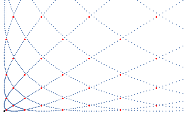
Figure 1: Illustration of the spectrum of Virasoro primaries in the $(h,\tilde{h})$ plane for $k=-12,c=-59.5$. The red dots correspond to the type $(r,1)\otimes(\tilde{r},1)$ primaries which an interpretation as solitons in the Lorentzian bulk theory. The black dot is the lowest lying primary of type $(1,|k|)\otimes(1,|k|)$.

The precise multiplicity $d(r,s;\tilde{r},\tilde{s})$ of the $(r,s)\otimes(\tilde{r},\tilde{s})$ representation can be read off from the character decomposition

$$Z=\sum_{r,\tilde{r}=1}^{\infty}\sum_{s,\tilde{s}=1}^{|k|}d(r,s;\tilde{r},\tilde{s})\chi_{r,s}\bar{\chi}_{\tilde{r},\tilde{s}},$$ (160)

and is given by, for $|k|$ even as in the case of interest,

$$d(r,s;\tilde{r},s)= 2r\tilde{r} {\rm for} \ s\notin\left\{{|k|\over 2},|k|\right\}\ {\rm and\ }r+\tilde{r}\ {\rm even}$$

$${}d(r,s;\tilde{r},|k|-s)= 2r\tilde{r} {\rm for} \ s\notin\left\{{|k|\over 2},|k|\right\}\ {\rm and\ }r+\tilde{r}\ {\rm odd}$$

$${}d\left(r,{|k|\over 2};\tilde{r},{|k|\over 2}\right)= 2r\tilde{r}$$

$${}d(r,|k|;\tilde{r},|k|)= r\tilde{r} {\rm for} \ r+\tilde{r}\ {\rm even}$$ (161)

Let us discuss the spectrum in more detail. As we argued previously, the primaries of type $(r,1)\otimes(\tilde{r},1)$ have a clear Lorentzian gravity interpretation as solitonic surplus solutions. These appear when $r+\tilde{r}$ is even, with multiplicity $2r\tilde{r}$. The remaining primary states do not have a clear interpretation as smooth Lorentzian solutions but have to be included in the theory to render it consistent. Similar to the momentum sectors of a standard compact boson, they do have an interpretation as winding sectors around the time direction in the Euclidean path integral.

It’s important to note that, while the spectrum of conformal weights is bounded below, there are states with negative weights. The state with lowest weights is the primary $(1,|k|)\otimes(1,|k|)$ with

$$h_{1,|k|}=\tilde{h}_{1,|k|}={c-1\over 24}.$$ (162)

which appears with multiplicity one. Since the energy scales with $c$ it is tempting to associate a classical background to this state, which we seem to be instructed to include in the theory. This would be the zero mass and angular momentum limit of the BTZ black hole metric, see (40). This solution is not smooth and the Chern-Simons gauge fields have a nontrivial holonomy of parabolic type.

It is well-known that in CFTs where the lowest-lying state is not the conformal vacuum, the central charge $c$ appearing in the Virasoro algebra is not the measure of the number degrees of freedom in the theory. The latter is rather measured by the effective central charge $c_{\rm eff}=c-24h_{\rm min}$ which is one in our case. This is the reason why the theory can have the same partition function (154) as a theory with $c=1$. The fact that $c_{\rm eff}=1$ explains why the theory does not contain BTZ black holes with finite horizon: while the spectrum does display Cardy growth with an exponential number of states at high level Cardy:1986ie , the entropy does not scale with Newton’s constant and is therefore too small to lead to a horizon in the bulk description. One can therefore think of these models as containing only gravitational solitons and no black holes.

4.4 The monster of log-ness

So far, we have discussed the $c_{|k|,1}$ models at the level of the partition function and its decomposition into irreducible characters. The fact that these models are in fact logarithmic CFTs is not so obvious from this point of view, though there are some indicators. A first notable feature is that most representations appear with multiplicities in the spectrum (cfr. the factor of 2 in (158)). Indeed, even the ‘vacuum’ representation with $h_{1,1}=\tilde{h}_{1,1}=0$ is apparently doubly degenerate. If the spectrum is degenerated, it can happen Gurarie:1993xq that $L_{0}$ (as well as the other zero-modes of the chiral algebra) are not diagonalizable but have nontrivial Jordan cells. For example $L_{0}$ might be represented on the two ‘vacuum’ states as the matrix

$$L_{0}=\left(\begin{array}[]{cc}0&1\\ 0&0\end{array}\right).$$ (163)

In this case, the two $h_{1,1}=0$ representations are part of a larger indecomposable module. Theories of this type are called logarithmic CFTs, and in fact the $c_{|k|,1}$ models under consideration are among the most studied examples (see Flohr:2001zs ; Gaberdiel:2001tr ; Creutzig:2013hma for reviews). The partition function is insensitive to the presence of Jordan cells like (163) and it still formally decomposes into irreducible characters. The actual representations however do not decompose into irreducibles and instead form indecomposable structures. Another hint of the logarithmic nature of the theory is the fact that the irreducible characters do not have nice transformation properties under modular group since the theta and affine theta functions in (141) have different weights under the modular $S$-transformation.

Though a thorough review of logarithmic CFTs is beyond the scope of this note, it is worth recalling how the logarithmic structure appears in the simplest example with $k=-2$ and $c=c_{2,1}=-2$ (which, as we recall from section 2, is strictly speaking not in our class of gravity models in which $k\in 4\mathbb{Z}$). The lightest degenerate primary field is ${\cal O}_{2,1}$ with $h_{2,1}=-1/8$. The four-point correlator of such fields is determined by a differential equation of second order which expresses the decoupling of the null vector at level two. In this special case the roots of the characteristic equation coincide which leads to a logarithmic branch of solutions. In terms of the OPE this translates into

$${\cal O}_{2,1}(z){\cal O}_{2,1}(0)\sim z^{-{1\over 4}}({\cal O}_{1,1}(0)+\log z{\cal O}_{1,1}^{\prime}(0))+\ldots$$ (164)

Here, ${\cal O}_{1,1}$ and ${\cal O}_{1,1}^{\prime}$ are two primary fields of weight $h_{1,1}=0$. The action of $L_{0}$ on the corresponding states yields precisely the Jordan form of (163):

$$L_{0}{\cal O}_{1,1}^{\prime}={\cal O}_{1,1},\qquad L_{0}{\cal O}_{1,1}=0.$$ (165)

Acting on ${\cal O}_{1,1}^{\prime}$ with the level 1 generators of the chiral algebra furthermore connects to the doublet of states ${\cal O}_{2,1},Q_{+}{\cal O}_{2,1}$ at $h_{2,1}=1$, schematically:

The detailed analysis of Gaberdiel:1996np shows that there are in this case are four consistent representations of the triplet algebra: two indecomposable ones (including the one we just sketched) and the irreducible representations which we called ${\cal H}^{W}_{1,2},{\cal H}^{W}_{2,2}$ before. The resulting CFT is rational in the sense that it has only a finite number of representations of the chiral algebra. Combining the holomorphic and antiholomorphic sectors into a local CFT leads to further nontrivial constraints as was discussed in Gaberdiel:1998ps . The upshot for the $|k|=2$ example, which presumably generalizes to arbitrary $|k|$, is that the entire last term containing the sum in (158) forms the character of a single indecomposable representation.

5 Discussion

In this work we made a case for a holographic dual interpretation of the non-unitary $c_{p,1}$ logarithmic models at large $p$. It is interesting to contrast the proposal for a holographic duality involving a specific CFT with recently studied instances of ‘imprecise’ holography where a gravity-like theory in the bulk is described by an average over an ensemble of CFTs. In the recent example of Afkhami-Jeddi:2020ezh ; Maloney:2020nni , as in the original work on pure gravity Maloney:2007ud the partition function is obtained by starting from the Virasoro character of the lowest energy state in the theory and performing a (regularized) sum over modular images. This leads, under natural assumptions, to a continuous spectrum characteristic of an ensemble average of CFTs. However, in theories with $c_{\rm eff}=1$, the procedure of modular averaging becomes much more subtle. Indeed, the standard expression for the modular average becomes ill-defined (see e.g. (2.3) in Benjamin:2020mfz ) in this case. Both the models we considered here and the proposal for a gravity dual to Liouville theory in Li:2019mwb have $c_{\rm eff}=1$, and this seems to be how these examples bypass the assumptions leading to an ensemble-averaged partition function. It would be interesting to understand how this works for other examples of precise holography such as tensionless string theory on AdS₃ Eberhardt:2018ouy .

We end by listing some remaining confusions and possible generalizations.

• While, as we have argued, the $(r,1)\otimes(\tilde{r},1)$ representations have a clear Lorentzian bulk interpretation, the same can not be said of the other representations which were needed to fill out a modular invariant spectrum. These arose from winding sectors around the time direction in the Euclidean gravitational path integral. It is at present not clear if these represent fluctuations of matter fields that we should add to the theory (as was the case in the example of Perlmutter:2012ds , where similar representations came from a Vasiliev-like scalar field Prokushkin:1998bq ), or whether they should be seen as somewhat exotic boundary graviton sectors.

• It is somewhat unsatisfying that, in the current work, the logarithmic character of the dual theory was not directly visible in the bulk, rather we were led to it by considering the modular invariant completion of the spectrum. It would be interesting to see a logarithmic branch (164) appearing in an amplitude computed in the bulk. This should happen for example in the four-point amplitude of the lowest lying primary in the theory, which in the bulk is represented as an $M=J=0$ BTZ metric.

• It would be interesting to understand better if the standard nonunitary minimal models with $c_{p,p^{\prime}}$ for $p>p^{\prime}>1$ also have a gravity-like dual interpretation at large negative central charge. One would expect that the $(r,1)$ representations still have an interpretation as surplus solutions. However, the structure of the degenerate representations and of the partition function is more complicated in this case, and perhaps a more sophisticated version of our arguments could lead to these models.

• It is expected that our observations can be extended to higher spin theories based on an $SL(N,\mathbb{R})\times SL(N,\mathbb{R})$ Chern-Simons theory in the bulk. It would be interesting to understand if one obtains, following the procedure of Cotler:2018zff and section 2 an analog of the geometric action for W_N coadjoint orbits. Also, the argument of Campoleoni:2017xyl picks out the value of the central charge

  $$c^{N}_{|k|,1}=(N-1)\left(1-N(N+1){(|k|-1)^{2}\over|k|}\right)$$ (166)

  which for integral $k$ is a limiting case of the central charge for W_N minimal models.

Appendix A Variational principle and boundary term

In this section we briefly review, following Henneaux:1987hz , the boundary terms which have to be added to (79) to obtain a well-defined variational principle. This requires that we specify, in addition to the quasi-periodic boundary conditions along the $\phi$-circle, boundary conditions at initial and final times (say, $t_{1}$ and $t_{2}$) and possibly add appropriate boundary terms. Naively, the action is stationary on solutions of the equations of motion (82) if we keep $X$ fixed at both endpoints:

$$\delta X(t_{1},\phi)=\delta X(t_{2},\phi)=0.$$ (167)

However, as stressed in Henneaux:1987hz , this is not correct as it imposes two independent conditions while $X$ only obeys a first-order equation in time. As was argued there, a natural boundary condition to impose is

$$\delta X(t_{1},\phi)=-\delta X(t_{2},\phi).$$ (168)

One checks that the action is stationary on solutions obeying this boundary conditions if we add the boundary term

$$S_{\rm bdy}=-{|k|\over 16\pi}\int_{0}^{2\pi}d\phi\left(X(t_{2},\phi)-X(t_{1},\phi)\right)\left(X^{\prime}(t_{2},\phi)+X^{\prime}(t_{1},\phi)\right).$$ (169)

The presence of this boundary term also solves a puzzle about gauge invariance of the on-shell action. Using the shift transformation (71) we can represent the surplus solutions either as

$$X=rx_{+}\qquad{\rm or}\qquad X=r\phi+c_{0}.$$ (170)

Without the boundary term, the first form would lead to vanishing on-shell action while the second would give

$$S_{\rm on-shell}=-{|k|n^{2}\over 4}(t_{2}-t_{1})$$ (171)

This is the physically expected answer as it equals minus the energy of the solution times the time interval. Adding the boundary however term both forms in (170) give the correct answer (171). The boundary term is required for on-shell gauge invariance because the gauge transformation linking the two solutions does not vanish at the endpoints $t_{1}$ and $t_{2}$, though it does respect the boundary condition (168) for an appropriate choice of the constant $c_{0}$ in (170).

References

- (1) A. Maloney and E. Witten, “Quantum Gravity Partition Functions in Three Dimensions,” JHEP 02 (2010) 029, arXiv:0712.0155 [hep-th].
- (2) N. Benjamin, H. Ooguri, S.-H. Shao, and Y. Wang, “Light-cone modular bootstrap and pure gravity,” Phys. Rev. D 100 no. 6, (2019) 066029, arXiv:1906.04184 [hep-th].
- (3) N. Benjamin, S. Collier, and A. Maloney, “Pure Gravity and Conical Defects,” JHEP 09 (2020) 034, arXiv:2004.14428 [hep-th].
- (4) H. Maxfield and G. J. Turiaci, “The path integral of 3D gravity near extremality; or, JT gravity with defects as a matrix integral,” arXiv:2006.11317 [hep-th].
- (5) A. Castro, M. R. Gaberdiel, T. Hartman, A. Maloney, and R. Volpato, “The Gravity Dual of the Ising Model,” Phys. Rev. D 85 (2012) 024032, arXiv:1111.1987 [hep-th].
- (6) C.-M. Jian, A. W. Ludwig, Z.-X. Luo, H.-Y. Sun, and Z. Wang, “Establishing strongly-coupled 3D AdS quantum gravity with Ising dual using all-genus partition functions,” JHEP 10 (2020) 129, arXiv:1907.06656 [hep-th].
- (7) E. Witten, “Three-Dimensional Gravity Revisited,” arXiv:0706.3359 [hep-th].
- (8) O. Coussaert, M. Henneaux, and P. van Driel, “The Asymptotic dynamics of three-dimensional Einstein gravity with a negative cosmological constant,” Class. Quant. Grav. 12 (1995) 2961–2966, arXiv:gr-qc/9506019 [gr-qc].
- (9) S. Li, N. Toumbas, and J. Troost, “Liouville Quantum Gravity,” Nucl. Phys. B952 (2020) 114913, arXiv:1903.06501 [hep-th].
- (10) D. Anninos and B. Mühlmann, “Matrix integrals finite holography,” arXiv:2012.05224 [hep-th].
- (11) P. Saad, S. H. Shenker, and D. Stanford, “JT gravity as a matrix integral,” arXiv:1903.11115 [hep-th].
- (12) S. Deser, R. Jackiw, and G. ’t Hooft, “Three-Dimensional Einstein Gravity: Dynamics of Flat Space,” Annals Phys. 152 (1984) 220.
- (13) S. Deser and R. Jackiw, “Three-Dimensional Cosmological Gravity: Dynamics of Constant Curvature,” Annals Phys. 153 (1984) 405–416.
- (14) A. Castro, R. Gopakumar, M. Gutperle, and J. Raeymaekers, “Conical Defects in Higher Spin Theories,” JHEP 02 (2012) 096, arXiv:1111.3381 [hep-th].
- (15) E. Perlmutter, T. Prochazka, and J. Raeymaekers, “The semiclassical limit of CFTs and Vasiliev theory,” JHEP 05 (2013) 007, arXiv:1210.8452 [hep-th].
- (16) J. Raeymaekers, “Quantization of conical spaces in 3D gravity,” JHEP 03 (2015) 060, arXiv:1412.0278 [hep-th].
- (17) A. Campoleoni, S. Fredenhagen, S. Pfenninger, and S. Theisen, “Asymptotic symmetries of three-dimensional gravity coupled to higher-spin fields,” JHEP 11 (2010) 007, arXiv:1008.4744 [hep-th].
- (18) M. Flohr, “Bits and pieces in logarithmic conformal field theory,” Int. J. Mod. Phys. A18 (2003) 4497–4592, arXiv:hep-th/0111228 [hep-th].
- (19) M. R. Gaberdiel, “An Algebraic approach to logarithmic conformal field theory,” Int. J. Mod. Phys. A18 (2003) 4593–4638, arXiv:hep-th/0111260 [hep-th].
- (20) D. Grumiller, W. Riedler, J. Rosseel, and T. Zojer, “Holographic applications of logarithmic conformal field theories,” J. Phys. A46 (2013) 494002, arXiv:1302.0280 [hep-th].
- (21) I. I. Kogan, “Singletons and logarithmic CFT in AdS / CFT correspondence,” Phys. Lett. B 458 (1999) 66–72, arXiv:hep-th/9903162.
- (22) A. Campoleoni, S. Fredenhagen, and J. Raeymaekers, “Quantizing higher-spin gravity in free-field variables,” JHEP 02 (2018) 126, arXiv:1712.08078 [hep-th].
- (23) J. Cotler and K. Jensen, “A theory of reparameterizations for AdS3 gravity,” JHEP 02 (2019) 079, arXiv:1808.03263 [hep-th].
- (24) R. Floreanini and R. Jackiw, “Selfdual Fields as Charge Density Solitons,” Phys. Rev. Lett. 59 (1987) 1873.
- (25) G. Felder, “BRST Approach to Minimal Models,” Nucl. Phys. B317 (1989) 215. [Erratum: Nucl. Phys.B324,548(1989)].
- (26) M. A. I. Flohr, “On modular invariant partition functions of conformal field theories with logarithmic operators,” Int. J. Mod. Phys. A11 (1996) 4147–4172, arXiv:hep-th/9509166 [hep-th].
- (27) M. R. Gaberdiel and H. G. Kausch, “A Rational logarithmic conformal field theory,” Phys. Lett. B386 (1996) 131–137, arXiv:hep-th/9606050 [hep-th].
- (28) P. Di Francesco, H. Saleur, and J. B. Zuber, “Modular Invariance in Nonminimal Two-dimensional Conformal Theories,” Nucl. Phys. B285 (1987) 454.
- (29) A. Achucarro and P. K. Townsend, “A Chern-Simons Action for Three-Dimensional anti-De Sitter Supergravity Theories,” Phys. Lett. B180 (1986) 89.
- (30) E. Witten, “(2+1)-Dimensional Gravity as an Exactly Soluble System,” Nucl. Phys. B311 (1988) 46.
- (31) J. D. Brown and M. Henneaux, “Central Charges in the Canonical Realization of Asymptotic Symmetries: An Example from Three-Dimensional Gravity,” Commun. Math. Phys. 104 (1986) 207–226.
- (32) J. Sonnenschein, “Chiral Bosons,” Nucl. Phys. B309 (1988) 752–770.
- (33) V. G. Drinfeld and V. V. Sokolov, “Lie algebras and equations of Korteweg-de Vries type,” J. Sov. Math. 30 (1984) 1975–2036.
- (34) S. Elitzur, G. W. Moore, A. Schwimmer, and N. Seiberg, “Remarks on the Canonical Quantization of the Chern-Simons-Witten Theory,” Nucl. Phys. B326 (1989) 108–134.
- (35) A. Campoleoni and S. Fredenhagen, “On the higher-spin charges of conical defects,” Phys. Lett. B726 (2013) 387–389, arXiv:1307.3745 [hep-th].
- (36) V. G. Kac, “Contravariant Form for Infinite Dimensional Lie Algebras and Superalgebras,” in Group theoretical methods in physics. proceedings, 7th international colloquium and integrative conference held in Austin, Texas, September 11-16, 1978, pp. 441–445. 1978.
- (37) J. M. Izquierdo and P. K. Townsend, “Supersymmetric space-times in (2+1) adS supergravity models,” Class. Quant. Grav. 12 (1995) 895–924, arXiv:gr-qc/9501018 [gr-qc].
- (38) T. Mansson and B. Sundborg, “Multi - black hole sectors of AdS(3) gravity,” Phys. Rev. D65 (2002) 024025, arXiv:hep-th/0010083 [hep-th].
- (39) J. de Boer, A. Castro, E. Hijano, J. I. Jottar, and P. Kraus, “Higher spin entanglement and conformal blocks,” JHEP 07 (2015) 168, arXiv:1412.7520 [hep-th].
- (40) E. Witten, “Coadjoint Orbits of the Virasoro Group,” Commun. Math. Phys. 114 (1988) 1.
- (41) A. Alekseev and S. L. Shatashvili, “Path Integral Quantization of the Coadjoint Orbits of the Virasoro Group and 2D Gravity,” Nucl. Phys. B323 (1989) 719–733.
- (42) G. W. Gibbons, S. W. Hawking, and M. J. Perry, “Path Integrals and the Indefiniteness of the Gravitational Action,” Nucl. Phys. B138 (1978) 141–150.
- (43) V. S. Dotsenko and V. A. Fateev, “Conformal Algebra and Multipoint Correlation Functions in Two-Dimensional Statistical Models,” Nucl. Phys. B240 (1984) 312.
- (44) D. Kapec and R. Mahajan, “Comments on the Quantum Field Theory of the Coulomb Gas Formalism,” arXiv:2010.10428 [hep-th].
- (45) M. Henneaux and C. Teitelboim, “Consistent quantum mechanics of chiral p forms,” in 2nd Meeting on Quantum Mechanics of Fundamental Systems (CECS) Santiago, Chile, December 17-20, 1987, pp. 79–112. 1987.
- (46) J. Balog, L. Feher, L. O’Raifeartaigh, P. Forgacs, and A. Wipf, “Toda Theory and Algebra From a Gauged WZNW Point of View,” Annals Phys. 203 (1990) 76–136.
- (47) M. Lavelle and D. McMullan, “A New symmetry for QED,” Phys. Rev. Lett. 71 (1993) 3758–3761, arXiv:hep-th/9306132 [hep-th].
- (48) D. J. Gross, J. A. Harvey, E. J. Martinec, and R. Rohm, “Heterotic String Theory. 1. The Free Heterotic String,” Nucl. Phys. B256 (1985) 253.
- (49) T. L. Curtright and C. B. Thorn, “Conformally Invariant Quantization of the Liouville Theory,” Phys. Rev. Lett. 48 (1982) 1309. [Erratum: Phys. Rev. Lett.48,1768(1982)].
- (50) B. L. Feigin and D. B. Fuks, “Verma modules over the Virasoro algebra,” Funct. Anal. Appl. 17 (1983) 241–241.
- (51) H. Kausch, “Extended conformal algebras generated by a multiplet of primary fields,” Phys. Lett. B 259 (1991) 448–455.
- (52) J. Polchinski, “Evaluation of the One Loop String Path Integral,” Commun. Math. Phys. 104 (1986) 37.
- (53) M. Henneaux and C. Teitelboim, Quantization of gauge systems. 1992.
- (54) P. H. Ginsparg, “Curiosities at c = 1,” Nucl. Phys. B 295 (1988) 153–170.
- (55) M. R. Gaberdiel and H. G. Kausch, “A Local logarithmic conformal field theory,” Nucl. Phys. B538 (1999) 631–658, arXiv:hep-th/9807091 [hep-th].
- (56) H. G. Kausch, “Curiosities at c = -2,” arXiv:hep-th/9510149 [hep-th].
- (57) J. L. Cardy, “Operator Content of Two-Dimensional Conformally Invariant Theories,” Nucl. Phys. B 270 (1986) 186–204.
- (58) V. Gurarie, “Logarithmic operators in conformal field theory,” Nucl. Phys. B 410 (1993) 535–549, arXiv:hep-th/9303160.
- (59) T. Creutzig and D. Ridout, “Logarithmic Conformal Field Theory: Beyond an Introduction,” J. Phys. A46 (2013) 4006, arXiv:1303.0847 [hep-th].
- (60) N. Afkhami-Jeddi, H. Cohn, T. Hartman, and A. Tajdini, “Free partition functions and an averaged holographic duality,” arXiv:2006.04839 [hep-th].
- (61) A. Maloney and E. Witten, “Averaging over Narain moduli space,” JHEP 10 (2020) 187, arXiv:2006.04855 [hep-th].
- (62) L. Eberhardt, M. R. Gaberdiel, and R. Gopakumar, “The Worldsheet Dual of the Symmetric Product CFT,” JHEP 04 (2019) 103, arXiv:1812.01007 [hep-th].
- (63) S. F. Prokushkin and M. A. Vasiliev, “Higher spin gauge interactions for massive matter fields in 3-D AdS space-time,” Nucl. Phys. B545 (1999) 385, arXiv:hep-th/9806236 [hep-th].