Motion Adaptive Deblurring with Single-Photon Cameras

Abstract

Single-photon avalanche diodes (SPADs) are a rapidly developing image sensing technology with extreme low-light sensitivity and picosecond timing resolution. These unique capabilities have enabled SPADs to be used in applications like LiDAR, non-line-of-sight imaging and fluorescence microscopy that require imaging in photon-starved scenarios. In this work we harness these capabilities for dealing with motion blur in a passive imaging setting in low illumination conditions. Our key insight is that the data captured by a SPAD array camera can be represented as a 3D spatio-temporal tensor of photon detection events which can be integrated along arbitrary spatio-temporal trajectories with dynamically varying integration windows, depending on scene motion. We propose an algorithm that estimates pixel motion from photon timestamp data and dynamically adapts the integration windows to minimize motion blur. Our simulation results show the applicability of this algorithm to a variety of motion profiles including translation, rotation and local object motion. We also demonstrate the real-world feasibility of our method on data captured using a $32\times 32$ SPAD camera.

1 Introduction

When imaging dynamic scenes with a conventional camera, the finite exposure time of the camera sensor results in motion blur. This blur can be due to motion in the scene or motion of the camera. One solution to this problem is to simply lower the exposure time of the camera. However, this leads to noisy images, especially in low light conditions. In this paper we propose a technique to address the fundamental trade-off between noise and motion blur due to scene motion during image capture. We focus on the challenging scenario of capturing images in low light, with fast moving objects. Our method relies on the strengths of rapidly emerging single-photon sensors such as single-photon avalanche diodes (SPADs).

Figure 1: Overview of our adaptive motion deblurring method. (a) The photon frames captured from a rotating fan contain timestamps for the first detected photon in each frame. Note the smaller value of timestamps in brighter regions and vice versa. (b) Flux changepoints obtained after changepoint detection and flux estimation at pixel location highlighted in cyan in (a). Note the rapidly varying photon timestamps due to heavy-tailed nature of the raw timestamp data. (c) A changepoint video (CPV) maintains sharp edges while providing motion cues to estimate inter-frame motion trajectories; the temporal flux profile of the highlighted pixel in this CPV is the piecewise constant function shown in (b). (d) Integrating photons along estimated spatio-temporal motion trajectories generates a sharp image with high signal-to-noise ratio.

Light is fundamentally discrete and can be measured in terms of photons. Conventional camera pixels measure brightness by first converting the incident photon energy into an analog quantity (e.g. photocurrent, or charge) that is then measured and digitized. When imaging in low light levels, much of the information present in the incident photons is lost due to electronic noise inherent in the analog-to-digital conversion and readout process. Unlike conventional image sensor pixels that require 100’s-1000’s of photons to produce a meaningful signal, SPADs are sensitive down to individual photons. A SPAD pixel captures these photons at an instant in time, with a time resolution of hundreds of picoseconds. Each photon detection can therefore be seen as an instantaneous event, free from any motion blur. Recently, single photon sensors have been shown to be useful when imaging in low light, or equivalently, imaging at high frame rates where each image frame is photon-starved [22].

The data captured by a SPAD camera is thus quite different than a conventional camera: in addition to the two spatial dimensions, we also capture data on a high resolution time axis resulting in a 3D spatio-temporal tensor of photon detection events. We exploit this novel data format to deal with the noise-blur trade-off. Our key observation is that the photon timestamps can be combined dynamically, across space and time, when estimating scene brightness. If the scene motion is known a priori, photons can be accumulated along corresponding spatio-temporal trajectories to create an image with no motion blur. A conventional camera does not have this property because at capture time high frequency components are lost [24]. So even with known scene motion, image deblurring is an ill-posed problem.

Our method relies on dynamically changing exposure times, where each pixel can have its own set of exposure times. An overview of our approach is shown in Fig. 1. We propose using statistical changepoint detection to infer points in time where the photon flux at a given pixel changes from one steady state rate to another. This allows us to choose exposure times that adapt to scene motion. Changepoints allow us to track high contrast edges in the scene and align “high frequency” motion details across multiple image frames. We show that for the case of global motion (e.g., rotation) we can track the varying motion speeds of different scene pixels and combine photons spatially to create deblurred images. We also show that for the case of local scene motion, our method can provide robust estimates of flux changepoints around the edges of the moving objects that improves deblurring results obtained from downstream motion alignment and integration.

The locations of changepoints can be thought of as a spike-train generated by a neuromorphic event camera [9], but with three key differences: First, unlike an event camera, our method preserves original intensity information for each pixel. Second, the numbers and locations of events, chosen by our algorithm, adapt to each pixel, without the need for a hard-coded change threshold. Third, direct photon measurements are inherently more sensitive, less noisy, and have a higher time resolution than conventional cameras. Current cameras create an analog approximation of the quantized photon stream (usually a charge level in a capacitor) and then measure and digitize that analog quantity. This process introduces noise and does not take advantage of the inherent quantized properties of the photons. We therefore expect photon counting methods to have higher sensitivity, accuracy, and temporal resolution than analog cameras, when imaging in low light scenarios.

Single-Photon Sensitive Cameras for Machine Vision? Currently, single-photon sensitive image sensors are quite limited in their spatial resolution compared to conventional complementary metal–oxide–semiconductor (CMOS) and charge-coupled device (CCD) image sensors. However, single-photon image sensing is a rapidly developing field; recent work has demonstrated the feasibility of making megapixel resolution single-photon sensitive camera arrays [23, 12]. Moreover, silicon SPAD arrays are amenable to manufacturing at scale using the same photolithographic fabrication techniques as conventional CMOS image sensors. This means that many of the foundries producing our cellphone camera sensors today could also make SPAD array sensors at similar cost. Other current limitations of SPAD sensors are the small fraction of chip area sensitive to light (fill factor) resulting from the large amount of additional circuitry that is required in each pixel. Emerging 3D stacking technologies could alleviate this problem by placing the circuitry behind the pixel.

Limitations Our experimental demonstration uses a first generation commercial SPAD array that is limited to a 32$\times$32 pixel spatial resolution. More recently 256$\times$256 pixel commercial arrays have become available [5]. Although current SPAD cameras cannot compete with the image quality of commercial CMOS and CCD cameras, with the rapid development of SPAD array technology, we envision our techniques could be applied to future arrays with spatial resolution similar to that of existing CMOS cameras.

Contributions:

• We introduce the notion of flux changepoints; these can be estimated using an off-the-shelf statistical changepoint detection algorithm.

• We show that flux changepoints enable inter-frame motion estimation while preserving edge details when imaging in low light and at high speed.

• We show experimental demonstration using data acquired from a commercially available SPAD camera.

2 Related Work

Motion Deblurring Motion deblurring for existing cameras can be performed using blind deconvolution [21]. Adding a fast shutter (“flutter shutter”) sequence can aid this deconvolution task [24]. We push the idea of a fluttered shutter to the extreme limit of individual photons: our image frames consist of individual photon timestamps allowing dynamic adaptation of sub-exposure times for the shutter function. Our deblurring method is inspired by burst photography pipelines used for conventional CMOS cameras. Burst photography relies on combining frames captured with short exposure times [16], resulting in large amounts of data that suffer from added readout noise. Moreover, conventional motion deblurring methods give optimal performance when the exposure time is matched to the true motion speed which is not known a priori.

Event-based Vision Sensors Event cameras directly capture temporal changes in intensity instead of capturing scene brightness [9]. Although it is possible to create intensity images from event data in post-processing [3], our method natively captures scene intensities at single-photon resolution: the “events” in our sensing modality are individual photons. The notion of using photon detections as “spiking events” has also been explored in the context of biologically inspired vision sensors [30, 1]. We derive flux changepoints from the high-resolution photon timestamp data. Due to the single-photon sensitivity, our method enjoys lower noise in low light conditions, and pixel-level adaptivity for flux changepoint estimation.

Deblurring Methods for Quanta Image Sensors There are two main single-photon detection technologies for passive imaging: SPADs [20, 17] and quanta image sensors (QIS) [8]. Although our proof-of-concept uses a SPAD camera, our idea of adaptively varying exposure times can be applied to QIS data as well. Existing motion deblurring algorithms for QIS [13, 14, 22] rely on a fixed integration window to sum the binary photon frames. However, the initial step of picking the size of this window requires a priori knowledge about the motion speed and scene brightness. Our technique is therefore complementary to existing motion deblurring algorithms. For example, our method can be considered as a generalization of the method in [18] which uses two different window sizes. Although we use a classical correlation-based method for motion alignment, the sequence of flux changepoints generated using our method can be used with state-of-the-art align-and-merge algorithms [22] instead.

3 SPAD Image Formation Model

SPADs are most commonly used in synchronization with an active light source such as a pulsed laser for applications including LiDAR and fluorescence microscopy. In contrast, here we operate the SPAD passively and only collect ambient photons from the scene. In this section, we describe the imaging model for a single SPAD pixel collecting light from a fixed scene point whose brightness may vary as a function of time due to camera or scene motion.

3.1 Pixelwise Photon Flux Estimator

Our imaging model assumes a frame-based readout mechanism: each SPAD pixel in a photon frame stores at most one timestamp of the first captured ambient photon. This is depicted in Fig. 1(a). Photon frames are read out synchronously from the entire SPAD array; the data can be read out quite rapidly allowing photon frame rates of 100s of kHz (frame times on the order of a few microseconds).

Let $N_{\text{pf}}$ denote the number of photon frames, and $T_{\text{pf}}$ be the frame period. So the total exposure time is given by $T=N_{\text{pf}}T_{\text{pf}}$. We now focus on a specific pixel in the SPAD array. In the $i^{\text{th}}$ photon frame ($1\leq i\leq N_{\text{pf}}$), the output of this pixel is tagged with a photon arrival timestamp $t_{i}$ relative to the start of that frame. If no photons are detected during a photon frame, we assume $t_{i}=T_{\text{pf}}$.

Photon arrivals at a SPAD pixel can be modeled as a Poisson process [15]. It is possible to estimate the intensity of this process (i.e. the perceived brightness at the pixel) from the sequence of photon arrival times [20, 17]. The maximum likelihood brightness estimator $\widehat{\Phi}$ for the true photon flux $\Phi$ is given by [20]:

$$\widehat{\Phi}=\frac{\sum_{i=1}^{N_{\text{pf}}}\mathbf{1}(t_{i}\neq T_{\text{pf}})}{q\sum_{i=1}^{N_{\text{pf}}}t_{i}}$$ (1)

where $q$ is the sensor’s photon detection efficiency and $\mathbf{1}$ denotes a binary indicator variable.

This equation assumes that the pixel intensity does not change for the exposure time $T$. The assumption is violated in case of scene motion. If we can determine the temporal locations of intensity changes, we can use still use Eq. (1) to estimate a time-varying intensity profile for each pixel. In the next section we introduce the idea of flux changepoints and methods to locate them with photon timestamps.

3.2 Flux Changepoints

Photon flux at a given pixel may change over time in case of scene motion. This makes it challenging to choose pixel exposure times a priori: ideally, for pixels with rapidly varying brightness, we should use a shorter exposure time and vice versa. We propose an algorithm that dynamically adapts to brightness variations and chooses time-varying exposure times on a per pixel basis. Our method relies on locating temporal change locations where the pixel’s photon flux has a large change: we call these flux changepoints.

In general, each pixel in the array can have different numbers and locations of flux changepoints. For pixels that maintain constant brightness over the entire capture period (e.g. pixels in a static background), there will be no flux changepoints detected and we can integrate photons over the entire capture time $T$. For pixels with motion, we assume that the intensity between flux changepoints is constant, and we call these regions virtual exposures. Photons in each virtual exposure are aggregated to create a piecewise constant flux estimate. The length of each virtual exposure will depend on how quickly the local pixel brightness varies over time, which in turn, depends on the true motion speed.

An example is shown in Fig. 1(b). Note that the photon timestamps are rapidly varying and extremely noisy due to a heavy-tailed exponential distribution. Our changepoint detection algorithm detects flux changepoints (red arrows) and estimates a piecewise constant flux waveform for the pixel (blue plot). In the example shown, five different flux levels are detected.

3.2.1 Changepoint Detection

Detecting changepoints is a well studied problem in the statistics literature [4, 26]. The goal is to split a time-series of measurements into regions with similar statistical properties. Here, our time series is a sequence of photon timestamps at a pixel location, and we would like to find regions where the timestamps have the same mean arrival rate, i.e., the photon flux during this time is roughly constant.

Using the sequence of photon arrival times $\{t_{i}\}_{i=1}^{N_{\text{pf}}}$, we wish to find a subset $\{t_{l_{1}},\ldots,t_{l_{L}}\}$ representing the flux changepoints. For convenience, we let the first and the last flux changepoint be the first and the last photons captured by the pixel ($l_{1}:=1$ and $l_{L}=N_{\text{pf}}$).

Offline changepoint detection is non-causal, i.e., it uses the full sequence of photon timestamps for a pixel to estimate flux changepoints at that pixel. In Suppl. Note S.1 we describe an online changepoint detection method that can be used for real-time applications.

For a sequence of photon timestamps, we solve the following optimization problem [29] (see Suppl. Note S.1):

$$(l_{i}^{*})_{i=1}^{L}\!=\!\operatorname*{arg\,min}_{l_{1},\!\ldots,\!l_{L}}\sum^{L-1}_{i=1}\!\left[-\log(\widehat{\Phi}_{i})\sum^{l_{i+1}}_{j=l_{i}}\mathbf{1}(t_{j}\!\neq\!T_{\text{pf}})\right]\!+\!\lambda L$$ (2)

where $\widehat{\Phi}_{i}$ is the photon flux estimate given by Eq. (1) using only the subset of photons between times $t_{l_{i}}$ and $t_{l_{i+1}}$. Here $\lambda$ is the penalty term that prevents overfitting by penalizing the number of flux changepoints. For larger test images we use the BottomUp algorithm [28] which is approximate but has a faster run time. For lower resolution images we use the Pruned Exact Linear Time (PELT) algorithm [19] which gives an exact solution but runs slower. See Suppl. Section S.4 for results using the BottomUp algorithm.

Flux Changepoints for QIS Data The cost function in Eq. (2) applies to photon timestamp data, but the same idea of adaptive flux changepoint detection can be used with QIS photon count data as well. A modified cost function that uses photon counts (0 or 1) is derived in Suppl. Note S.1.2.

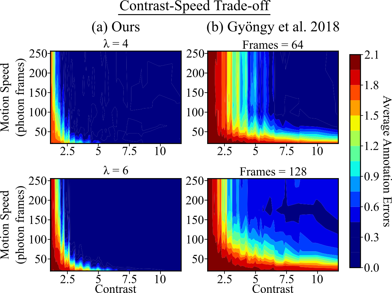
Figure 2: Contrast-Speed Trade-off. We simulate a single SPAD pixel measuring a pulse-shaped photon flux signal to analyze the contrast-speed trade-off when detection motion. Our method (a) based on PELT changepoint detection adapts to a wider range of contrast and speed combinations than the comparison method (b) from Gyöngy et al. [14].

3.2.2 Single-Pixel Simulations

There is a trade-off between contrast and motion speed when trying to detect changepoints. For example, it is harder to detect the flux change with a fast moving object with a lower contrast with respect to its background. To evaluate this trade-off, we simulate a single SPAD pixel for 800 photon frames with a time varying flux signal with a randomly placed pulse wave. We use the pulse width as a proxy for motion speed, and vary the contrast by varying the ratio of the pulse height. We measure the absolute difference between the number of changepoints detected by our algorithm and the true number of flux changes (which is exactly 2 for a single pulse). We call this “annotation error.”

Fig. 2 shows the annotation errors for different values of contrast and motion speeds for two different algorithms. For each set of contrasts and motion speeds we display the average number of annotation errors over 120 simulation runs. We use the PELT algorithm to detect flux changepoints. For comparison, we also show the fixed windowing approach used by Gyöngy et al. [14, 2]. The changepoint detection algorithm is able to adapt to a wider range of contrasts and speeds.

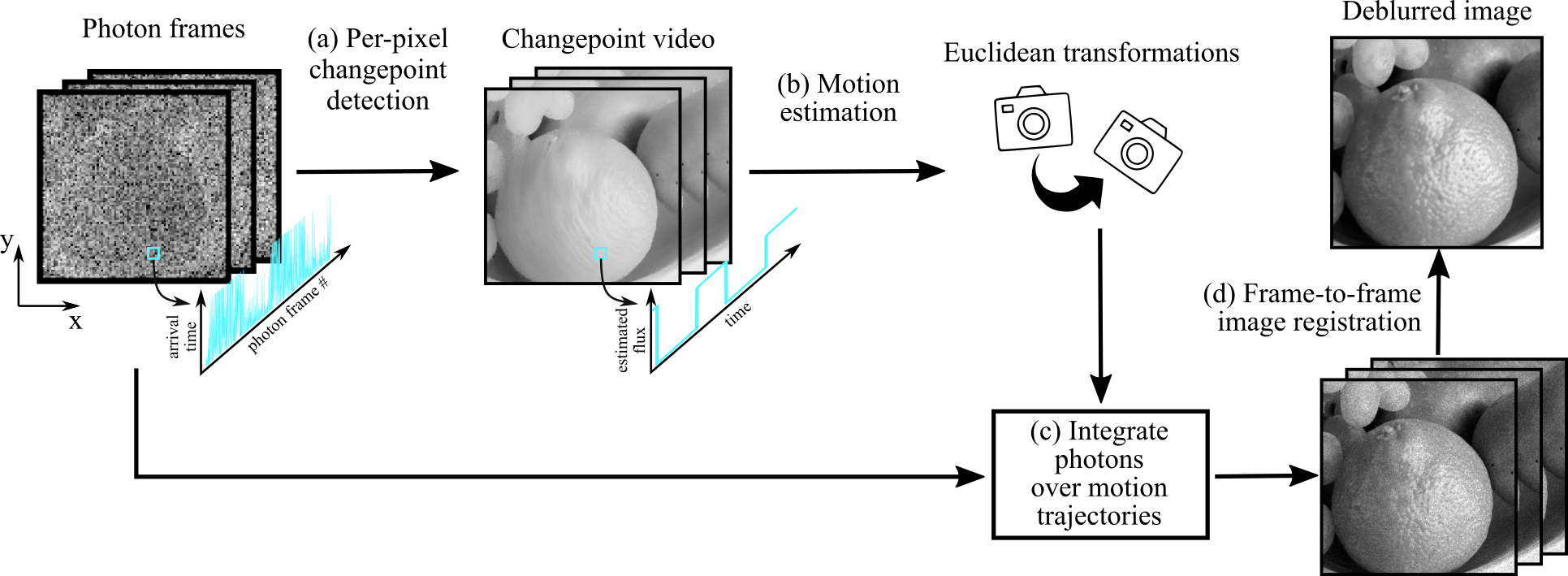
Figure 3: Changepoint video deblurring. Photon timestamps for each pixel location in the 3D timestamp tensor are analyzed for changepoints (a) to generate a changepoint video. Pixels may have different numbers of changepoints, and hence, dynamically changing frame-rate over time. We estimate motion between successive frames of the changepoint video (b) and estimate motion parameters. Finally, using this motion estimate, we sum photons (c) from the photon frames along motion trajectories resulting in a deblurred video. Frames in the deblurred video are registered and summed (d) to obtain the final deblurred image. (Original images from FreeImages.com)

4 Pixel-Adaptive Deblurring

4.1 Changepoint Video

Using methods described in the previous section we locate flux changepoints for each pixel in the image. The changepoints for each pixel represent when a new virtual exposure starts and stops; photons within each virtual exposure can be used to estimate photon flux using Eq. (1). We call this collection of piecewise constant functions over all pixels in the array the changepoint video (CPV).

The CPV does not have an inherent frame rate; since each pixel has a continuous time piecewise constant function, it can be sampled at arbitrarily spaced time instants in $[0,T]$ to obtain any desired frame rate. We sample the CPV at non-uniform time intervals using the following criterion. Starting with the initial frame sampled at $t=0$, we sample the subsequent frames at instants when at least 1% of the pixel values have switched to a new photon flux. This leads to a variable frame rate CPV that adapts to changes in scene velocity: scenes with fast moving objects will have a higher average CPV frame rate.

The CPV preserves large brightness changes in a scene. For example, the edges of a bright object moving across a dark background remain sharp. However, finer texture details within an object may appear blurred.

4.2 Spatio-Temporal Motion Integration

We use global motion cues from the CPV and then combine the motion estimates with the photon frames to create a deblurred video. The overall flowchart is shown in Fig. 3.

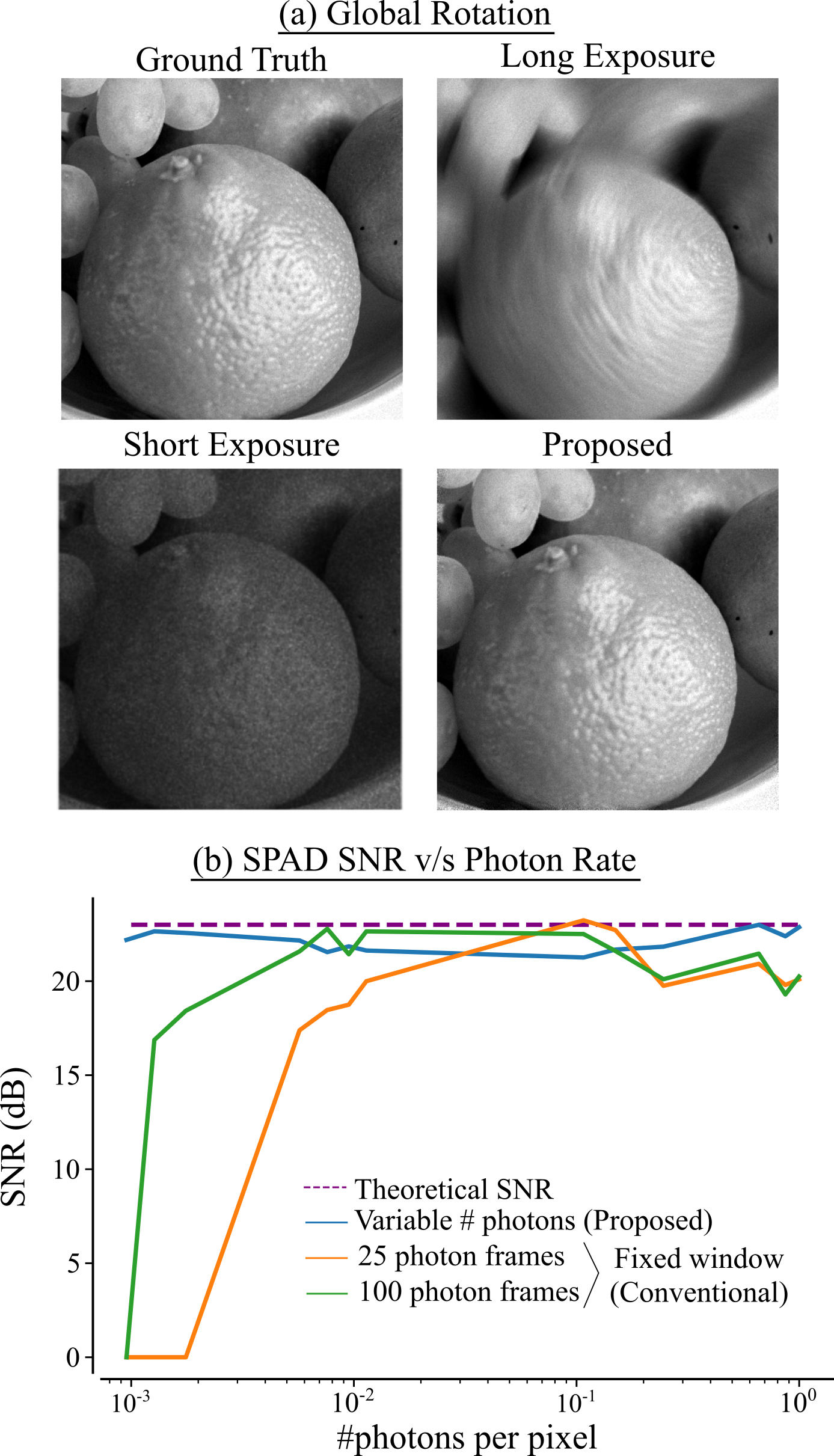
Figure 4: Comparison of SNR for different deblurring window sizes. (a) A ground truth video of a rotating orange used for creating simulated SPAD photon frames. A long exposure image is quite blurry while a short exposure image is very noisy. Our deblurring algorithm strikes a balance between noise and blur to get a sharp high-quality image. (b) By varying the brightness of the orange scene, we compare the simulated SNR using our method compared to a conventional method with fixed windows. Notice the proposed method stays above 20 dB at all photon rates, while the fixed photon window SNRs decrease in the low photon count regime. (Original image from FreeImages.com)

We use a correlation-based image registration algorithm to find the motion between consecutive frames in the CPV. For each location $\mathbf{p}=[x,y]$ in the $i^{\text{th}}$ CPV frame, we assume it maps to a location $\mathbf{p}^{\prime}$ in $(i+1)^{\text{st}}$ CPV frame. We assume that the mapping is a linear transformation:

$$A\mathbf{p}=\mathbf{p}^{\prime}.$$ (3)

We constrain $A$ to represent planar Euclidean motion (rotation and translation). Let $\theta$ be the amount of rotation centered around a point $[r_{x},r_{y}]$ and let $[\tau_{x},\tau_{y}]$ be the translation vector. Then $A$ has the form:

$$A\!=\!\begin{bmatrix}\cos\theta&\sin\theta&r_{x}(1\!-\!\cos\theta)\!+\!r_{y}\sin\theta\!+\!\tau_{x}\\ -\sin\theta&\cos\theta&r_{y}(1\!-\!\cos\theta)\!-\!r_{x}\sin\theta\!+\!\tau_{y}\\ 0&0&1\end{bmatrix}.$$ (4)

We apply the enhanced correlation coefficient maximization algorithm [7] to estimate the transformation matrix $A$ for consecutive pairs of CPV frames $i\rightarrow i+1$. A sequence of frame-to-frame linear transformations generates arbitrarily shaped global motion trajectories. We aggregate the original photon frame data along these estimated spatio-temporal motion trajectories.

We assume that the rotation center, $[r_{x},r_{y}]$, is the middle of the image and a change in rotation center can be modeled as a translation. We solve for $\theta$, $\tau_{x}$, and $\tau_{y}$ which we linearly interpolate. Then using the interpolated motion parameters and Eq. (3), we align all photon frames corresponding to the time interval between CPV frames $i\rightarrow i+1$ and sum these frames to get a photon flux image by using Eq. (1) at each pixel. This generates a motion deblurred video with the same frame rate as the CPV, but with finer textures preserved as shown in Fig. 3.

If the final goal is to obtain a single deblurred image, we repeat the steps described above on consecutive frames in the deblurred video, each time decreasing the frame rate by a factor of 2, until eventually we get a single image. This allows us to progressively combine photons along spatial-temporal motion trajectories to increase the overall signal to noise ratio (SNR) and also preserve high frequency details that were lost in the CPV.

Our method fails when motion becomes too large to properly align images, especially at low resolutions. It can also fail when not many flux changepoints are detected, this will occur mainly due to a lack of photons per pixel of movement. In the worst case, if not enough changepoints are detected, the result of the algorithm will look similar to a single long exposure image.

The method of aligning and adding photon frames is similar to contrast maximization algorithms used for event cameras [10]. However, unlike event camera data, our method relies on the CPV which contains both intensity and flux changepoints derived from single-photon timestamps.

Handling Multiple Moving Objects To handle multiple moving objects on a static background, we implement a method similar to Gyögny et al. [14] and combine it with our CPV method. We cluster the changepoints for different objects using a density-based spatial clustering algorithm (DBSCAN) [6]. For each cluster, we then create a bounding box, isolating different moving objects. We then apply our motion deblurring algorithm on each object individually, before stitching together each object with the areas that are not moving in the CPV. The clustering step also denoises by rejecting flux changepoints not belonging to a cluster.

4.3 Simulations

Starting with a ground truth high resolution, high frame rate video, we scale the video frames to units of photons per second and generate photon frames using exponentially distributed arrival times. We model a photon frame readout SPAD array with $8000$ bins and bin width of $256\text{\,}\mathrm{ps}$.

We first simulate a rotating orange by applying successive known rigid transformations to an image and generating SPAD data by scaling the transformed images between $10^{4}$ and $10^{8}$ photons per second. We rotate the image by 0.1^∘ for every 10 generated photons for a total of 1000 photons. We use the BottomUp algorithm [29] with $\lambda=5$ for the changepoint detection step. The results are shown in Fig. 4(a). Our method captures sharp details on the orange skin while maintaining high quality.

Fig. 4(b) shows quantitative comparisons of SNR for different deblurring methods. The conventional approach to deblur photon data uses a fixed frame rate; we use two different window lengths for comparison. We compute the SNR of the deblurred imaging using the $\ell 2$ (root-mean-squared) distance from the ground truth to and repeat this over a range of photon flux levels. We keep the total number of photons captured approximately constant by extending the capture time for darker flux levels. Our method dynamically adapts to motion and lighting so we are able to reconstruct with high SNR even in photon starved regimes where the SNR of the fixed window methods degrades rapidly.

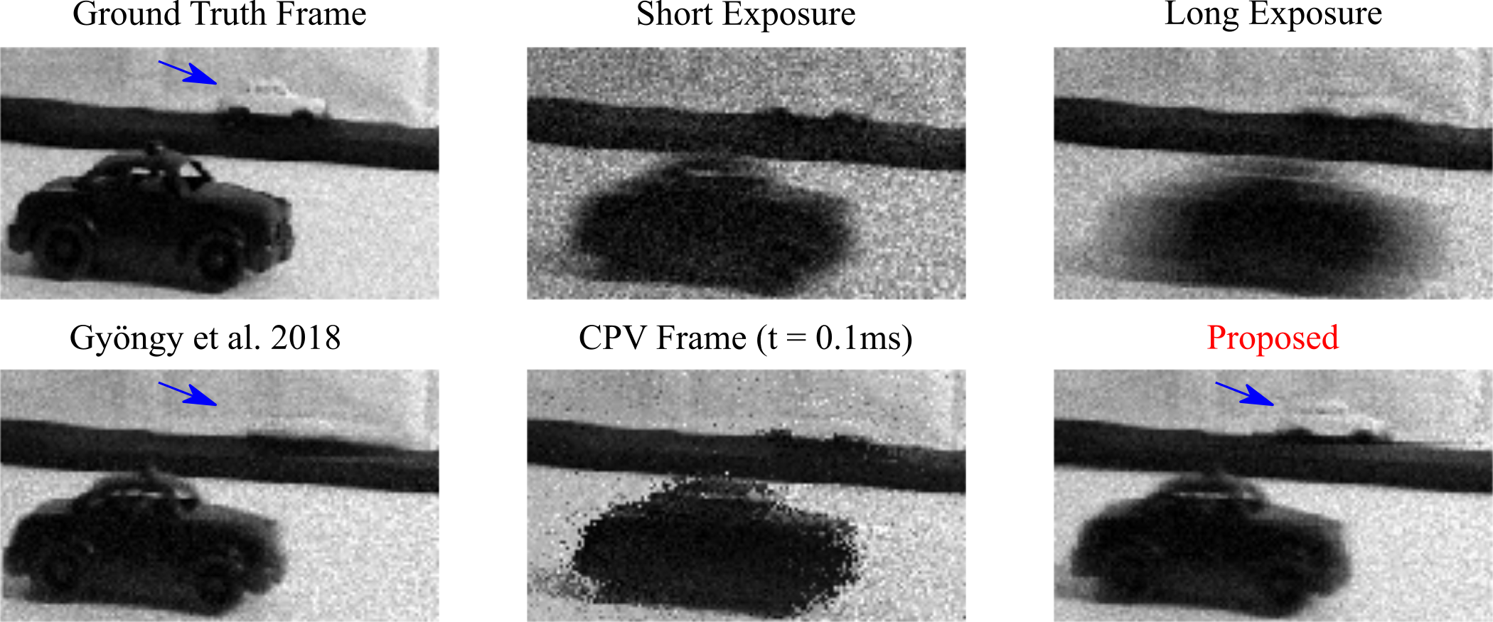
Figure 5: Simulated Motion Deblurring for Multiple Moving Objects. We simulate SPAD data from video of toy cars, a fast moving black car and slow moving white car. (Top row) A sample frame from the ground truth frame sequence is shown. The short and long exposure images show the results of using integrating the first 75 and 250 photon frames, respectively. Notice that the short exposure preserves the black car while the white car is quite noisy, on the other hand, the long average blurs the black car but preserves details of the white one better. (Bottom row) The method of Gyögny et al. [14], fails to reconstruct the white car (blue arrow) due to its low contrast. A sample frame from our changepoint video shows both moving cars. Finally, our deblurring algorithm is able to reconstruct both the black and white car with negligible motion blur.

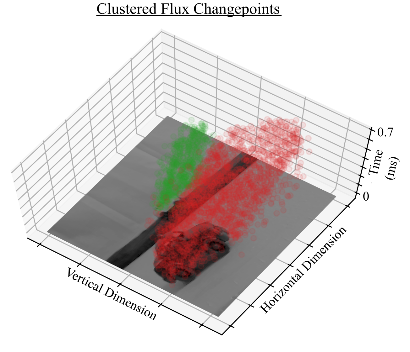
Figure 6: Clustered Flux Changepoints Two clusters of flux changepoints are detected using frames from the changepoint video for the toy car scene. These changepoint clusters are used for segmenting the moving cars from the static background.

To simulate multi-object motion, we captured a ground truth video of two toy cars rolling down a ramp at different speeds. The video frame pixels are then scaled between $10^{5}$ and $10^{6}$ photons per second and a total of 690 photon frames are generated. A bright slow moving car has a contrast of 1.2 with respect to the background, and moves 48 pixels over the duration of video. The dark car has a contrast of 5.0 with the background, and moves 143 pixels. We use the PELT algorithm [19] with $\lambda=6$ for the changepoint detection step. We use $\epsilon=7.5$ and $\text{MinPts}=40$ in the DBSCAN clustering algorithm. The resulting deblurred images are shown in Fig. 5. Observe that the method of [14] blurs out the low contrast white car in the back. Our method assigns dynamically changing integration windows extracted from the CPV to successfully recover both cars simultaneously with negligible motion blur. The changepoint clusters used for segmenting cars from the static background in our method are are shown in Fig. 6.

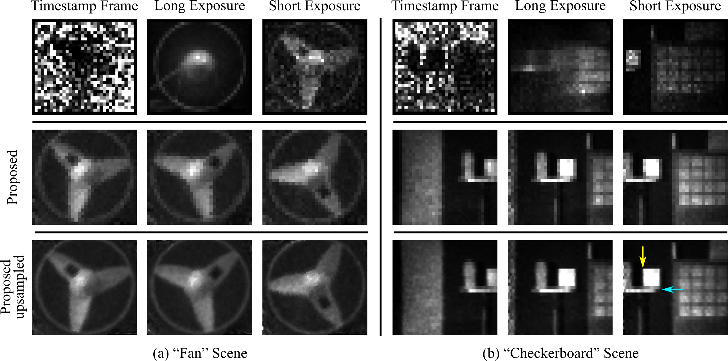
Figure 7: Experimental Results. The first row shows a single raw data frame from the photon timestamp tensor; each photon has an associated timestamp with a $250\text{\,}\mathrm{ps}$ bin resolution. Integration over a long exposure ($2\text{\,}\mathrm{ms}$ for the fan and $0.2\text{\,}\mathrm{ms}$ for checkerboard scene) this gives a low noise but blurry result. Using a short exposure time ($40\text{\,}\mathrm{\SIUnitSymbolMicro s}$ for both scenes) produces very noisy results. The second row shows a sequence of three frames from the final deblurred video. The third row shows the result with upsampling. Note that in the checkerboard scene due to purely horizontal motion, some vertical edges (yellow arrow) are sharper but not the horizontal edges (cyan arrow). See supplementary video results.

5 Experiments

We validate our method using experimental data captured using a 32$\times$32 InGaAs SPAD array from Princeton Lightwave Inc., USA. The pixels are sensitive to near infrared and shortwave infrared ($900\text{\,}\mathrm{nm}$–$1.6\text{\,}\mathrm{\SIUnitSymbolMicro m}$ wavelengths). The SPAD array operates in a frame readout mode at 50,000 photon frames per second. Each photon frame exposure window is $2\text{\,}\mathrm{\SIUnitSymbolMicro s}$ and sub-divided into 8000 bins, giving a temporal resolution of $250\text{\,}\mathrm{ps}$ per bin [27].

For this low resolution experimental data, we zero-order hold upsample both the timestamp frames and the CPV before step (b) in Fig. 3 in the spatial dimensions. We then use upsampled photon frames for step (c) resulting in sharper images. Upsampling before motion integration allows photons that are captured in the same pixel to land in a larger space during the motion integration step.

Fig. 7 shows results from two different scenes. The “fan” scene shows the performance of our algorithm with fast rotation. The optimal exposure time in this case depends on the rotation speed. Our method preserves the details of the fan blades including the small black square patch on one of the fan blades. The “checkerboard” scene shows deblurring result with purely horizontal global motion. Note that our method is able to resolve details such as the outlines of the squares on the checkerboard.

The last row in Fig. 7 shows the upsampled results. Benefits of upsampling are restricted to the direction of motion. The “fan” dataset is upsampled 9$\times$ compared to the original resolution. The “checkerboard” dataset is upsampled 4$\times$; this is because the motion is limited to the horizontal dimension. Note that some of the details in the vertical edges are sharp, but horizontal edges remain blurry.

6 Discussion and Future Work

Euclidean Motion Assumption In the case of camera shake, most of the motion will come from small rotations in the camera that result in 2D translations and rotations in the image frames. The short distance translations of shaking camera would cause translations in the frames that are similar in nature, but smaller in magnitude.

Translation of the camera over larger distances would result in parallax while motion within the scene can result in more complex changes. In these cases our model captures scene changes only approximately. It applies to frame to frame motion over short time-scales and limited to regions in the scene. Ideas for extending our model to deal with larger motion will be the subject of future work.

Dealing with Local Motion The techniques presented in this paper assume multiple moving objects exhibiting euclidean motion, with no occlusions. We can extend our approach to more complex motions. We can use a patch-wise alignment and merging methods to deal with more complex local motion and occlusions [16, 22].

Deblurring algorithms developed for event camera data can be adapted to SPAD data, because the flux changepoints represent changes in brightness similar to the output of event cameras. Current event camera algorithms are able to recover complex motion in scenes [10, 25], and they could be improved with a fusion based approach where image intensity information is also available [11].

Data Compression With increasing number of pixels, processing photon frames with high spatio-temporal resolution will be quite resource intensive. Our online changepoint method takes some initial steps towards a potential real-time implementation. The CPV can be used for video compression with variable frame rate: by tuning the regularization parameter of the changepoint detection algorithm a tradeoff between image fidelity and data rate can be achieved.

Acknowledgments This material is based upon work supported by the Department of Energy / National Nuclear Security Administration under Award Number DE-NA0003921, the National Science Foundation (GRFP DGE-1747503, CAREER 1846884), DARPA (REVEAL HR0011-16-C-0025) and the Wisconsin Alumni Research Foundation.

Disclaimer This report was prepared as an account of work sponsored by an agency of the United States Government. Neither the United States Government nor any agency thereof, nor any of their employees, makes any warranty, express or implied, or assumes any legal liability or responsibility for the accuracy, completeness, or usefulness of any information, apparatus, product, or process disclosed, or represents that its use would not infringe privately owned rights. Reference herein to any specific commercial product, process, or service by trade name, trademark, manufacturer, or otherwise does not necessarily constitute or imply its endorsement, recommendation, or favoring by the United States Government or any agency thereof. The views and opinions of authors expressed herein do not necessarily state or reflect those of the United States Government or any agency thereof.

S.1 Flux Changepoint Detection

S.1.1 Offline Algorithm: Cost Function Derivation

Consider a set of photon time stamp measurements $\{x_{i}\}_{i=1}^{N}$. Here each $x_{i}$ is a valid measurement, and in the frame-readout capture mode, described in the main text, this is different than the $t_{i}$’s. If no photon is detected in a frame we add the frame length to the next detected photon. We do this so each $x_{i}$ will be i.i.d. and distributed exponentially. We again wish to find a set of change points, $\{x_{l_{1}},\ldots,x_{l_{L}}\}$. In general, the optimization problem for changepoint detection is given by Eq. (P2) in rupturesPaper:

$$(l_{i}^{*})_{i=1}^{L}\!=\!\operatorname*{arg\,min}_{l_{1},\!\ldots,\!l_{L}}\sum^{L-1}_{i=1}\!c(x_{l_{i}...l_{i+1}}).\!+\!\lambda L$$ (S1)

The summation term represents the likelihood that each segment in between changepoints come from the same underlying distribution, while the regularization term is needed because the number of changepoints are not known a priori. For our case $c(\cdot)$ is the negative log likelihood for a set of exponentially distributed measurements. Let $f(x)$ be the exponential density function with rate parameter $\Phi$, and let $\widehat{\Phi}_{i}$ be the maximum likelihood estimate for $\Phi$ for the set of measurements $\{x_{l_{i}}\ldots x_{l_{i+1}}\}$. Note that the maximum likelihood estimator maximizes the log likelihood. To derive $c(\cdot)$, we begin with Eq. (C1) from rupturesPaper:

$$c(x_{l_{i}...l_{i+1}}) =-\underset{\Phi}{\max}\sum_{j=l_{i}}^{l_{i+1}}\log f(x_{j}|\Phi)$$ (S2)

$$=-\sum_{j=l_{i}}^{l_{i+1}}\log f(x_{j}|\widehat{\Phi}_{i})$$ (S3)

$$=-\sum_{j=l_{i}}^{l_{i+1}}\log\widehat{\Phi}_{i}e^{-\widehat{\Phi}_{i}x_{j}}$$ (S4)

$$=-\sum_{j=l_{i}}^{l_{i+1}}\log\widehat{\Phi}_{i}+\sum_{j=l_{i}}^{l_{i+1}}\widehat{\Phi}_{i}x_{j}$$ (S5)

$$=-(l_{i+1}-l_{i})\log\widehat{\Phi}_{i}+(l_{i+1}-l_{i})$$ (S6)

where the last line comes from the fact that $\widehat{\Phi}_{i}=\frac{(l_{i+1}-l_{i})}{\sum_{j=l_{i}}^{l_{i+1}}x_{j}}$. Plugging Eq. (S6) into Eq. (S1), the last term sums to a constant $N$ and can be dropped from the optimization. Then we convert to the direct measurments $t_{i}$ by expanding out where no photons where found to get Eq. (2).

S.1.2 QIS: Offline Cost Function

A quanta image sensor (QIS) is another sensor type capable of measuring single photons. Unlike a SPAD, the QIS senor only gives a binary output for each photon-frame corresponding to whether or not a photon was detected. Note that we can convert our experimental SPAD data to QIS data by stripping the SPAD data of the timing information. Let $n_{i}=0$ if the $i^{th}$ QIS photon-frame detects no photons and $n_{i}=1$ otherwise. Let $\tau_{b}$ be the temporal bin width for each photon-frame. Suppose the jot is exposed to a flux of $\Phi$, then the probability of detecting a photon during photon-frame $i$ is:

$$p=P(n_{i}=1)=1-e^{-q\Phi\tau_{b}}$$ (S7)

Where $q$ is the quantum efficiency. We can model measuring multiple photon-frames with the QIS jot as a Bernoulli Trial, with probability of success given by Eq. S7. For a set of $N$ photon-frames the maximum likelihood estimator, $\hat{\Phi}_{QIS}$, is given by ingle2019high,

$$\hat{\Phi}_{QIS}=\frac{-1}{q\tau_{b}}\ln({1-\widehat{p}})$$ (S8)

$$\widehat{p}=\frac{\sum_{i=0}^{N}n_{i}}{N}$$ (S9)

This flux estimator should also be used in SPAD sensors under very high fluxes, where their is significant probability of detecting more than one photon in a period equal to the SPAD’s time quantization. Similarly, the MLE in Eq. 1 can be used in low light conditions for a QIS sensor.

We derive the changepoint cost function in the raw data domain. Following the steps of the earlier derivation, with $f(n_{i})$ being the Bernoulli distribution with parameter $p$:

$$c_{QIS}(x_{l_{i}...l_{i+1}}) =-\underset{\Phi}{\max}\sum_{j=l_{i}}^{l_{i+1}}\log f(n_{j}|\Phi)$$ (S10)

$$=-\sum_{j=l_{i}}^{l_{i+1}}\log f(n_{j}|\widehat{\Phi}_{i})$$ (S11)

$$=-\log(\widehat{p_{i}})\sum_{j=l_{i}}^{l_{i+1}}n_{j}-\log(1-\widehat{p_{i}})\sum_{j=l_{i}}^{l_{i+1}}1-n_{j}$$ (S12)

Where $\widehat{p_{i}}=\frac{\sum_{j=l_{i}}^{l_{i+1}}n_{j}}{l_{i+1}-l_{i}}$.

S.1.3 Online Flux Changepoint Detection Algorithm

Offline changepoint detection is suitable for offline applications that capture a batch of photon frames and generate a deblurred image in post-processing. In some applications that require fast real-time feedback (e.g. live deblurred video) or on-chip processing with limited frame buffer memory, online changepoint detection methods can be used. We use a Bayesian online changepoint detection method Adams2007BayesianOC. This algorithm calculates the joint probability distribution of the time since the last flux changepoint. For exponentially distributed data, it uses the posterior predictive distribution which is a Lomax distribution (see Suppl. Note S.1.3). We assume that the flux changepoints appear uniformly randomly in the exposure window $T$. Because detecting a flux changepoint after only one photon is difficult we use a look-behind window that evaluates the probability of the photon 20–40 photon frames into the past as being a flux changepoint. Using a look-behind window greatly increases detection accuracy and introduces only minor latency (on the order of tens of microseconds). We also found that it is helpful to use a small spatial window that spreads out flux changepoints in space to increase the density of changepoints. In general, online detection will work better for slower motion as the algorithm learns from past data. We compare online and offline detection in Suppl. Note S.3.

We use a Bayesian changepoint detection algorithm shown in Algorithm 1 of Adams2007BayesianOC. Here we derive the posterior predictive distribution used in Step 3 of their algorithm. We use a $\textsf{Gamma}(\alpha,\beta)$ prior for $\Phi$. Let $\mathbf{x}:=\{x_{i}\}_{i=1}^{N}.$ It can be shown that $\Phi|\mathbf{x}\sim\textsf{Gamma}(\alpha+N,\beta+\sum_{i=1}^{N}x_{i})$. The predictive posterior density is given by:

$$f_{x_{N+1}|\mathbf{x}}(y|\mathbf{x}) =\int_{0}^{\infty}f_{x_{N+1}|\mathbf{\Phi}}(y|\Phi)f_{\mathbf{\Phi}|\mathbf{x}}(\Phi|{\bf x})d\Phi$$ (S13)

$$=\int_{0}^{\infty}\Phi e^{-\Phi y}\frac{(\beta+\sum x_{i})^{\alpha+N}}{\Gamma(\alpha+N)}\Phi^{\alpha+N-1}e^{-(\beta+\sum_{i}x_{i})\Phi}d\Phi$$ (S14)

$$=\frac{(\beta+\sum_{i}x_{i})^{\alpha+N}(\alpha+N)}{(\beta+y+\sum_{i}x_{i})^{\alpha+N-1}}$$ (S15)

which is a Lomax density with shape parameter $\alpha+N$ and scale parameter $\beta+\sum_{i}x_{i}$. For our data we used a $\mathsf{Lomax}(1,100)$ in Step 3 and $H(\cdot)=40$ in Steps 4 and 5 of Algorithm 1 in Adams2007BayesianOC.

For online detection we use code modified from onlineDetectionCode (Commit: 7d21606859feb63eba6d9d19942938873915f8dc). Fig. 1 shows the results of using the online changepoint detection algorithm. Observe that some of the edge details are better preserved with the offline changepoint algorithm.

We run the same experiment as in Fig. 4, where an orange is rotated at different brightness levels. We show the resulting SNR for online vs offline detection in supplementary Fig. 2

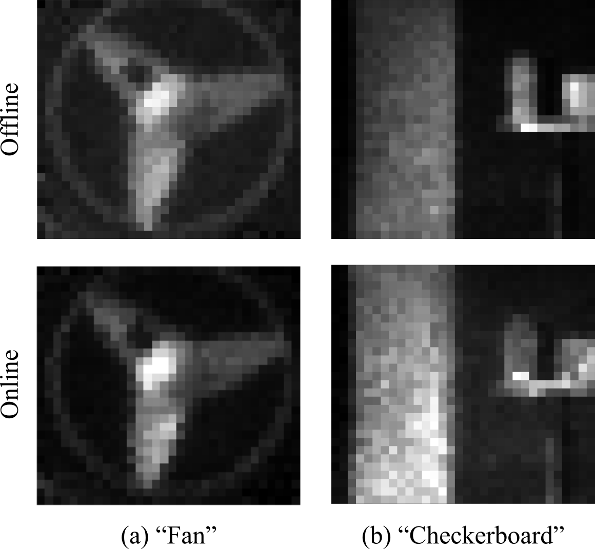
Supplementary Figure 1: Comparing online vs. offline changepoint detection. We processed the two experimental datasets using our online and offline changepoint detection algorithms. There is a slight loss of edge details when the online algorithm is used.

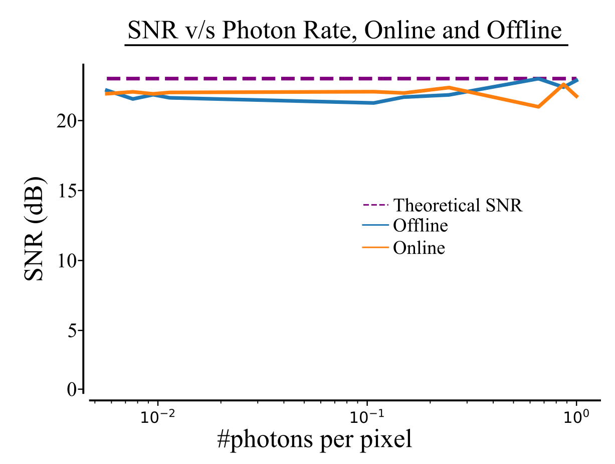
Supplementary Figure 2: Online vs. Offline Rotating Orange SNR We run the same experiment as in Fig. 4, with the rotating orange at many light levels. Note that the resulting SNRs of the two methods are quite similar.

S.2 SNR Analysis

We test our deblurring algorithm for different motion speeds for the case of rotational motion using the “orange” dataset in the main text. We measure the SNR by computing the discrepancy between the ground truth flux image and the deblurred result. We do this by temporally downsampling the original photon frames, so the number of photons decrease as the motion speeds up. Suppl. Fig. 3 shows how changing the regularization parameter $\lambda$ in the offline flux changepoint detection algorithm effects the SNR. We find that as long as $\lambda$ is high enough a good reconstruction SNR stays high. In Suppl. Fig. 4 we show that our algorithm converges to the performances of a long exposure capture (with motion blur) if the number of photons per degree of rotation falls below 3.

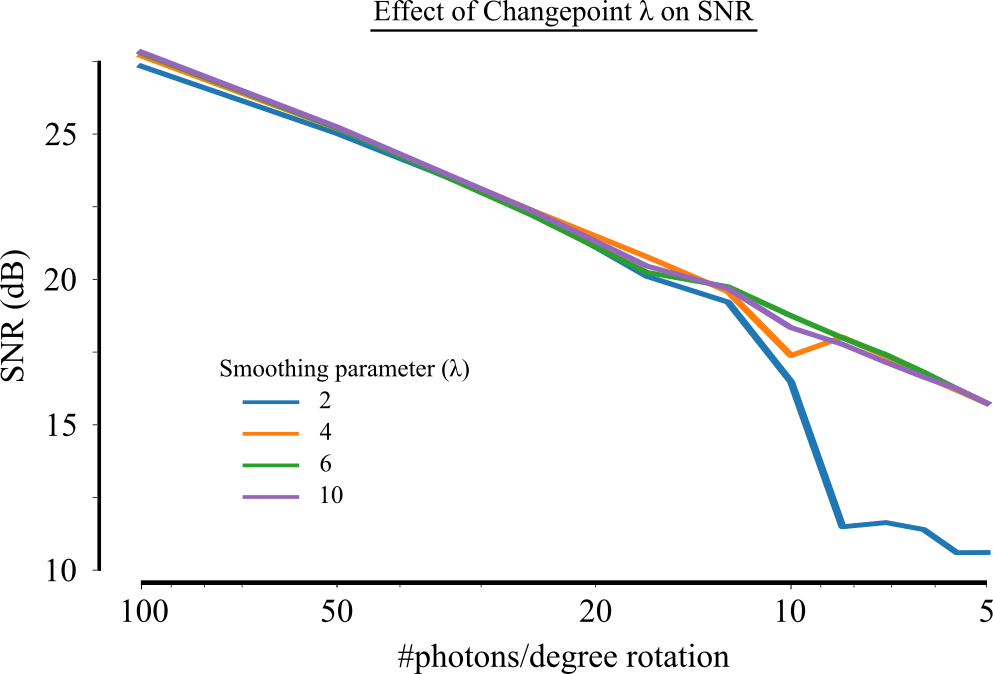
Supplementary Figure 3: Effect of offline changepoint algorithm regularization parameter $\lambda$. If $\lambda$ is large enough we get good performance. When $\lambda$ is too small, many flux changepoints are found, which will cause the CPV to be too noisy to properly align frames.

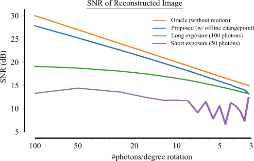
Supplementary Figure 4: Effect of number of photons captured per degree of rotation. Our algorithm is unable to find flux changepoints at speeds of 3 photon frames per degree. When no flux changepoints are found we just get a long exposure image. We also see that the SNR for a blurry image (long exposure) or a noisy image (short exposure) is worse than the proposed deblurring method until our method converges to the long exposure image.

We run the same experiment as in Fig. 4, where an orange is rotated at different brightness levels. We test our offline QIS changepoint detection method by removing the timing information and only considering a binary output. Our adaptive changepoint method helps at low light levels, see Fig. 5.

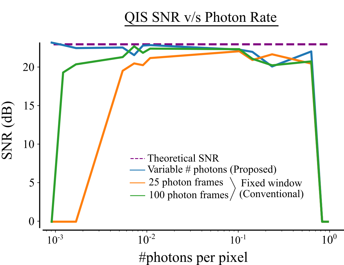
Supplementary Figure 5: QIS, SNR vs. Brightness. We run the same experiment as in Fig. 4, with the rotating orange at many light levels. We remove timing information from the raw data to create QIS binary data frames and run the same deblurring experiment. Again our adaptive changepoint method is helpful in low light scenarios. Note that the sharp drop on the right is due to saturation of a QIS sensor.

S.3 Additional Simulation Results

This section contains some additional simulated results. A second scene with two toy cars is displayed, we use the same parameters as the toy car scene in the main text for frame generation, changepoint detection and deblurring. For this scene the dark car moves 90 pixels and has a contrast 3.3. The bright car has a contrast of 1.2 and moves 30 pixels. Our results are shown in supplementary Fig. 6 and the clustered changepoints are shown in supplementary Fig. 7. Again, our method is able to deblur both moving cars.

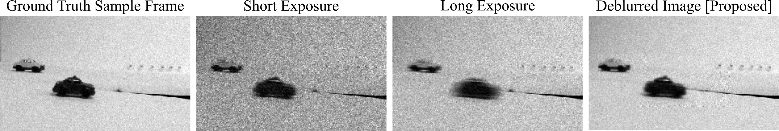
Supplementary Figure 6: Simulated Multiple Objects. We simulate SPAD data from a 240 fps phone video of two rolling toy cars, a fast moving dark car and slow moving bright car. From left to right, the ground truth image shows the result of generating the same number of photon frames from the first frame of the video sequence. The short and long exposure images show the results of using only the first 75 and 250 photon frames, respectively. Notice that the short exposure preserves the dark car while the bright car is quite noisy, on the other hand, the long average blurs the dark car but preserves details of the bright one better. Finally, our deblurring algorithm is able to reconstruct both the dark and bright car.

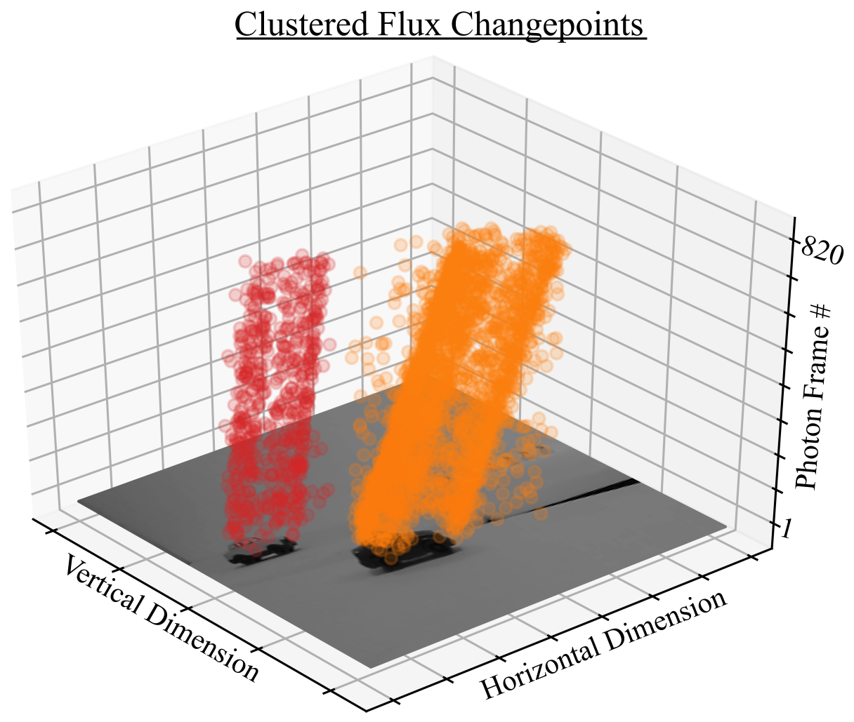
Supplementary Figure 7: Clustered Flux Changepoints Displayed are the 2 flux changepoint clusters found for the scene in Supplementary Fig. 6. We only display half of the flux changepoints in each cluster for visualization purposes.

We simulate a simple pixel art scene to demonstrate the advantage of deblurring on a changepoint video rather than burst frames. Notice in supplementary Fig. 8 that the changepoint video frame is able to capture a wide range of motion speeds and contrasts that a single fixed frame cannot capture.

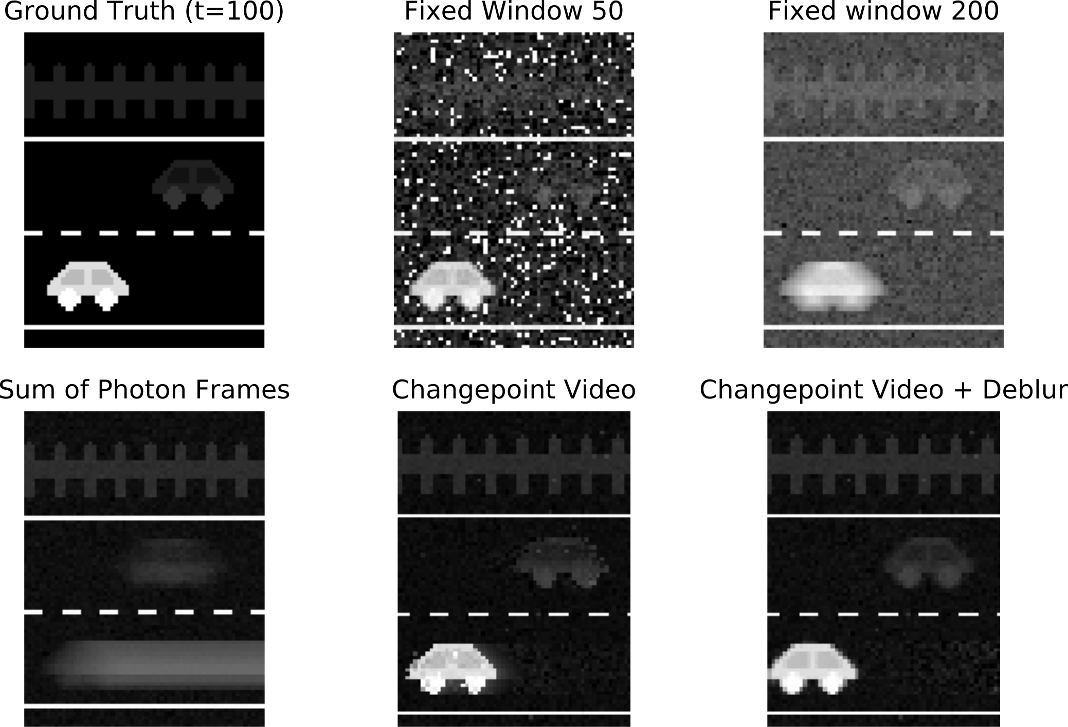
Supplementary Figure 8: Pixel Art Multiple Objects. We simulate a scene where a bright car moves quickly to the right and a dim car moves slowly to the left. Notice that in the short averaging window, the dim car is lost in the noise while in the long averaging window the bright car is blurred. The sum of all photon frames maintains the background quite well. The changepoint video frame adapts to motion in each pixel and captures both the bright car, the dim car, and the background. Notice that the changepoint video frame loses some of the structure of the dim car due to noisy changepoints. We combine the adaptive changepoint video with a deblurring algorithm to deblur both cars.

S.3.1 Global Motion Results

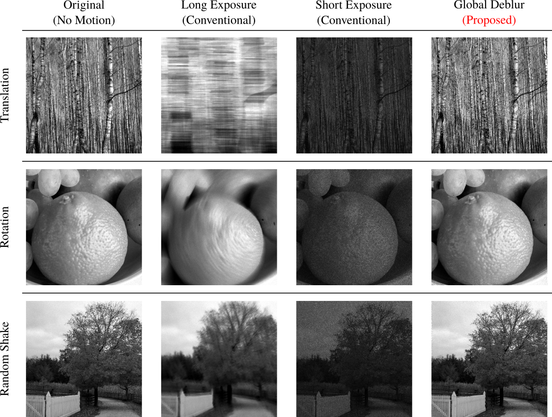
Supplementary Figure 9: Simulated motion deblurring results for different types of global motion. From left the right the columns show, a ground truth image that shows the result if the same number of photons are sampled from the original image but with no motion. A long exposure where all photon frames are summed, the result is a blurred image. A short exposure image shows the combination of the first 20 photons of the timestamp data, notice the edges are sharp but noise dominates. The result of the global motion deblur algorithm is shown in the last column. (Original images from FreeImages.com)

We start with a ground truth high resolution image, successively apply rigid transformations (using known rotations and translations), and generate photon frames using exponentially distributed arrival times. We reassign these high spatial resolution timestamps a lower resolution 2D array to simulate a low resolution SPAD pixel array.

We model a photon frame readout from a SPAD array with $8000$ bins and bin width of $256\text{\,}\mathrm{ps}$. Images are scaled so that the true photon flux values ranges between $10^{4}$ and $10^{8}$ photons per second. We then iteratively transform the flux image according to known motion parameters, and downsample spatially to a resolution of 425$\times$425 before generating photon timestamps.

For the horizontal translation blur, we moved the image 1 pixel to the right blur, we rotate the image 0.1 degree for every 10 generated photons for a total of 1000 photons. To emulate random camera shake, we create random motion trajectories by drawing two i.i.d. discrete uniform random variables between $-3$ and $3$ and use that as the number of pixels to translate along the horizontal and vertical directions. We generate 20 photons per translation for a total of 2000 photons. We use the BottomUp algorithm rupturesPaper with $\lambda=5$ for the changepoint detection step. In practice we found that the results were not very sensitive to the choice of $\lambda$ and values between $2$ and $12$ produced similar results.

We generate photon events from an exponential distribution. We transform the flux image, then down-sample to simulate objects with more detail than pixel resolution. We then generate 10-20 photons from the down-sampled flux image. Continuing this we get a 3-d tensor of photons representing global motion of the original image.

Supplementary Fig. 9 shows simulated deblurring results for three different motion trajectories. The top row shows a case of horizontal translation: conventional long/short exposures must trade off motion blur and shot noise. Our deblurring method reproduces sharp details, such as vertical lines of the tree stems. The second row shows a case of rotation: note that different pixels of the scene now undergo different amount of motion per unit time. Our method reconstructs fine details of the texture of the orange peel. The bottom row shows random camera shake with unstructured motion. Our technique is able to correct for this global motion by approximating the overall motion trajectory as a sequence of small translations and rotations. Supplementary Fig. 10 shows the comparison between the true motion trajectory and the trajectory estimated as part of our deblurring algorithm.

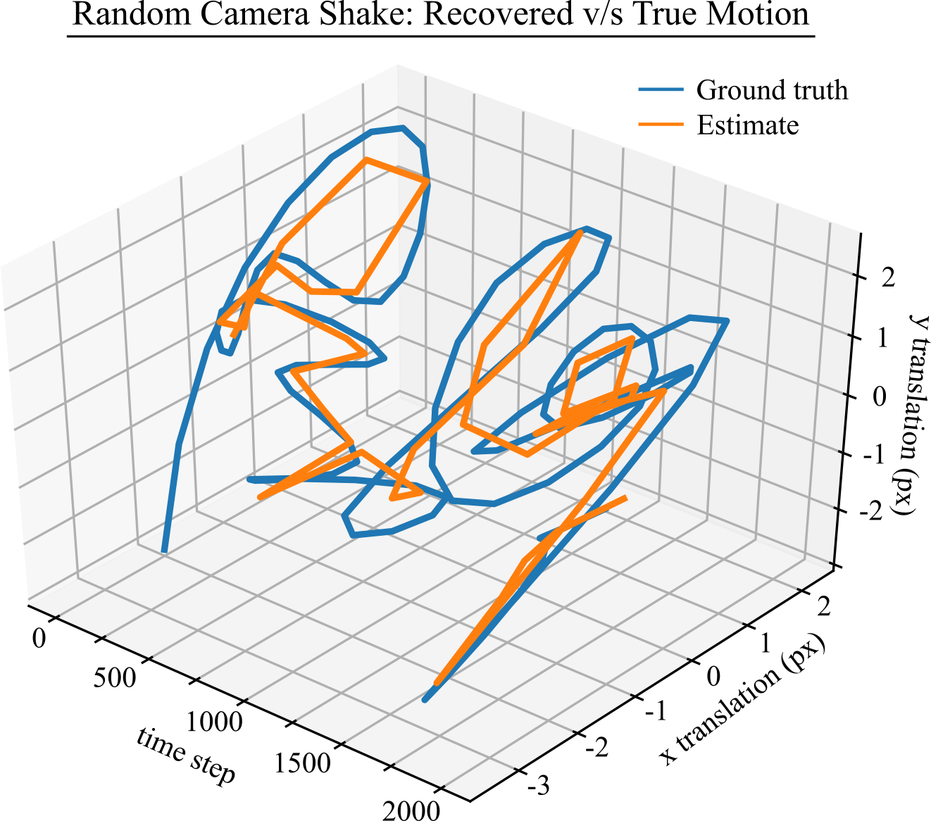
Supplementary Figure 10: Comparison of estimated and true motion trajectories. This plot shows the true and estimated motion trajectories for the random shake case in Fig. 9. The recovered motion tracks the ground truth motion quite well.

S.4 Comparison of BottomUp and PELT

In this section we run some of the same simulation experiments from the main text but with the BottomUp algorithm instead of the PELT algorithm. In Suppl. Fig. 11 we compare the ability of both algorithms on the toy car scene, BottomUp seems to produce slightly more noisy and blurry results. In Suppl. Fig. 12 we re-run the contrast vs. speed simulations and find that BottomUp does comparably well with slightly more false positives.

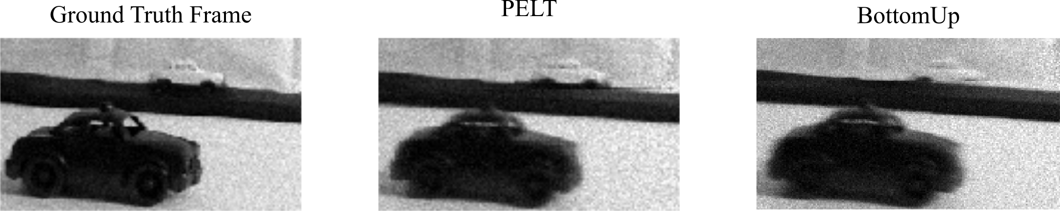
Supplementary Figure 11: Toy Car Simulated Scene. Here are the results using the toy car simulated scene. The parameters used are the same as in the main text. Note that the BottomUp algorithm is able to detect and deblur both cars; however, it seems to produce a slightly noisier and blurrier result. For this scene 210 by 300 with 690 photon frames per pixel, on our unoptimized system with 30 parallel cores, it takes the PELT algorithm two minutes to run while the BottomUp takes approximately one minute.

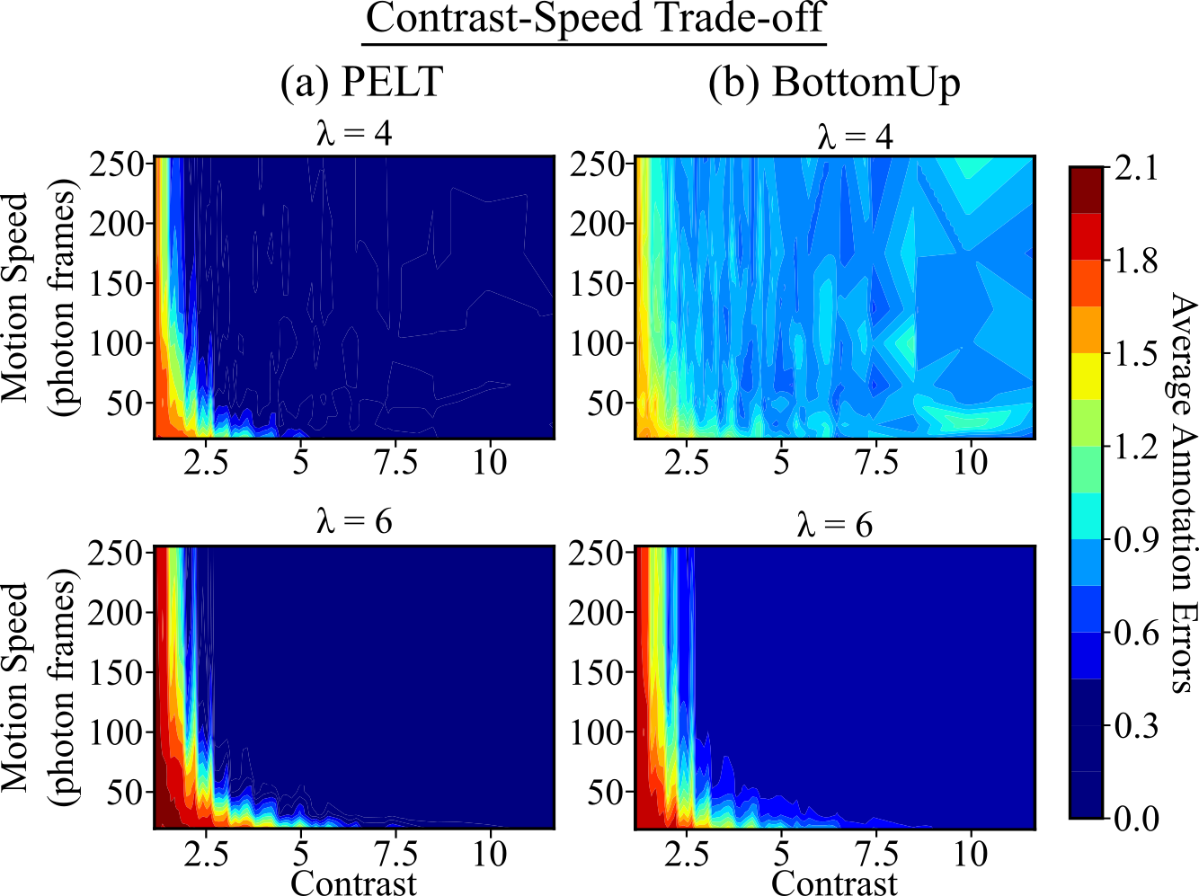
Supplementary Figure 12: BottomUp vs. PELT - Contrast vs. Speed. We repeat the contrast vs. speed simulation as done in the main text but with the BottomUp algorithm. Note that the BottomUp algorithm does comparably well for $\lambda=6$. For $\lambda=4$, the BottumUp algorithm is able to detect more difficult objects at the expense of false positives during easier scenarios.

S.5 Experiment Setup

For the experimental investigation we used a 32$\times$32 InGaAs SPAD array from Princeton Lightwave (PL GM-APD 32 x 32 Geiger-Mode Flash 3-D LiDAR Camera) and an RGB camera (VIS/BW point gray Grashopper 3, GS3-U3-23S6M-C) capturing the same field-of-view. The SPAD camera samples photon events with a depth of $10^{13}$ bins and $250\text{\,}\mathrm{p}\mathrm{s}\mathrm{/}\mathrm{b}\mathrm{i}\mathrm{n}$. Further, during the experiments we used a frame readout rate of $50\text{\,}\mathrm{k}\mathrm{H}\mathrm{z}$. The InGaAs sensor is sensitive in near infrared (NIR) to shortwave infrared (SWIR) wavelengths ranging from $900\text{\,}\mathrm{nm}$ to $1.6\text{\,}\mathrm{\SIUnitSymbolMicro m}$.

During the measurements we investigated two different type of scene setups: a “fan” and a “checkerboard” scene, as depicted in Suppl. Fig. 13. In the first scene, the fan consists of three blades mounted on a central cone and is enclosed by a circular frame with a diameter of $18\text{\,}\mathrm{cm}$. One blade was marked with a black piece of paper. The fan scene was used to investigate rotational motion. The second scene consists of an artificial head, a white plate and a colored checkerboard. Colors appear at a different gray levels in the SWIR wavelength images. This second scene was used to investigate random motion due to a horizontally shaking camera.

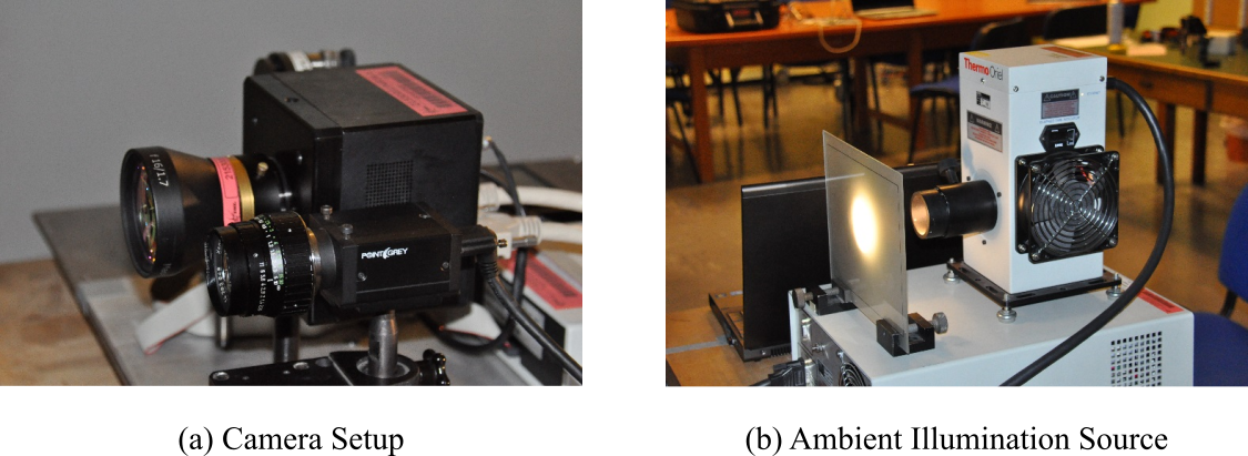
Supplementary Figure 13: Hardware setup (a) Our hardware setup consists of a Princeton Lightwave SPAD array (PL GM-APD 32$\times$32 Geiger-Mode Flash 3-D LiDAR Camera) and an RGB camera (VIS/BW point gray Grashopper 3, GS3-U3-23S6M-C) capturing the same field-of-view. (b) Ambient illumination is provided by a diffuse light source (broadband arc lamp ThermoOriel Model 66881).

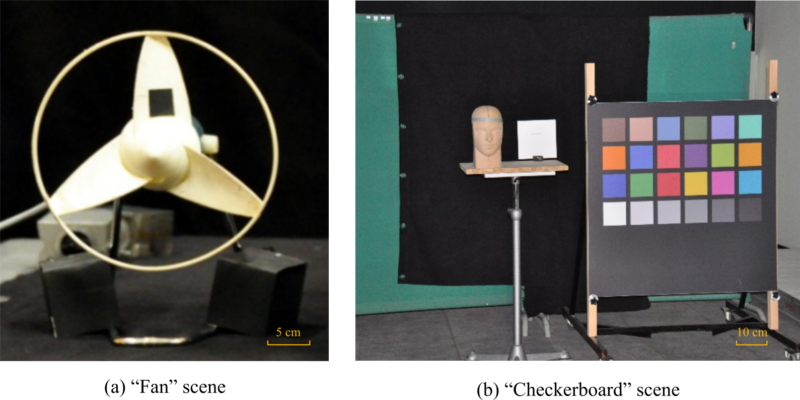
Supplementary Figure 14: Experimental Scenes (a) The “fan” scene consists of a small fan with a black square patch on one of the fan blades. (b) The “checkerboard” scene consists of a large color checkerboard and a mannequin head.

S.6 Description of Video Results

Please refer to included .txt and .mp4 files for supplementary video results. ieee_fullname egbib

References

- [1] S. Afshar, T. J. Hamilton, L. Davis, A. Van Schaik, and D. Delic. Event-based processing of single photon avalanche diode sensors. IEEE Sensors Journal, pages 1–1, 2020.
- [2] Alan Agresti and Brent A. Coull. Approximate is better than ”exact” for interval estimation of binomial proportions. The American Statistician, 52(2):119–126, 1998.
- [3] Patrick Bardow, Andrew J Davison, and Stefan Leutenegger. Simultaneous optical flow and intensity estimation from an event camera. In Proceedings of the IEEE Conference on Computer Vision and Pattern Recognition, pages 884–892, 2016.
- [4] Michèle Basseville, Igor V Nikiforov, et al. Detection of abrupt changes: theory and application, volume 104. Prentice Hall Englewood Cliffs, 1993.
- [5] Vinit Dhulla, Sapna S Mukherjee, Adam O Lee, Nanditha Dissanayake, Booshik Ryu, and Charles Myers. 256 x 256 dual-mode cmos spad image sensor. In Advanced Photon Counting Techniques XIII, volume 10978, page 109780Q. International Society for Optics and Photonics, 2019.
- [6] Martin Ester, Hans-Peter Kriegel, Jörg Sander, and Xiaowei Xu. A density-based algorithm for discovering clusters in large spatial databases with noise. In Proceedings of the Second International Conference on Knowledge Discovery and Data Mining, KDD’96, page 226–231. AAAI Press, 1996.
- [7] Georgios D Evangelidis and Emmanouil Z Psarakis. Parametric image alignment using enhanced correlation coefficient maximization. IEEE Transactions on Pattern Analysis and Machine Intelligence, 30(10):1858–1865, 2008.
- [8] Eric R Fossum, Jiaju Ma, Saleh Masoodian, Leo Anzagira, and Rachel Zizza. The quanta image sensor: Every photon counts. Sensors, 16(8):1260, 2016.
- [9] G. Gallego, T. Delbruck, G. M. Orchard, C. Bartolozzi, B. Taba, A. Censi, S. Leutenegger, A. Davison, J. Conradt, K. Daniilidis, and D. Scaramuzza. Event-based vision: A survey. IEEE Transactions on Pattern Analysis and Machine Intelligence, pages 1–1, 2020.
- [10] Guillermo Gallego, Henri Rebecq, and Davide Scaramuzza. A unifying contrast maximization framework for event cameras, with applications to motion, depth, and optical flow estimation. Proceedings / CVPR, IEEE Computer Society Conference on Computer Vision and Pattern Recognition. IEEE Computer Society Conference on Computer Vision and Pattern Recognition, 06 2018.
- [11] Daniel Gehrig, Henri Rebecq, Guillermo Gallego, and Davide Scaramuzza. EKLT: Asynchronous, photometric feature tracking using events and frames. Int. J. Comput. Vis., 2019.
- [12] Abhiram Gnanasambandam, Omar Elgendy, Jiaju Ma, and Stanley H Chan. Megapixel photon-counting color imaging using quanta image sensor. Optics express, 27(12):17298–17310, 2019.
- [13] I. Gyöngy, T. A. Abbas, N. Dutton, and R. Henderson. Object tracking and reconstruction with a quanta image sensor. In Proceedings of the International Image Sensor Workshop, 2017.
- [14] Istvan Gyongy, Neale AW Dutton, and Robert K Henderson. Single-photon tracking for high-speed vision. Sensors, 18(2):323, 2018.
- [15] Samuel W. Hasinoff. Photon, Poisson Noise, pages 608–610. Springer US, Boston, MA, 2014.
- [16] Samuel W Hasinoff, Dillon Sharlet, Ryan Geiss, Andrew Adams, Jonathan T Barron, Florian Kainz, Jiawen Chen, and Marc Levoy. Burst photography for high dynamic range and low-light imaging on mobile cameras. ACM Transactions on Graphics (TOG), 35(6):1–12, 2016.
- [17] Atul Ingle, Andreas Velten, and Mohit Gupta. High flux passive imaging with single-photon sensors. In Proceedings of the IEEE Conference on Computer Vision and Pattern Recognition, pages 6760–6769, 2019.
- [18] Gyongy Istvan, Dutton Neale, Luca Parmesan, Davies Amy, Saleeb Rebecca, Duncan Rory, Rickman Colin, Dalgarno Paul, and Robert K Henderson. Bit-plane processing techniques for low-light, high speed imaging with a spad-based qis. In International Image Sensor Workshop, pages 1–4, 2015.
- [19] R. Killick, P. Fearnhead, and I. A. Eckley. Optimal detection of changepoints with a linear computational cost. Journal of the American Statistical Association, 107(500):1590–1598, 2012.
- [20] Martin Laurenzis. Single photon range, intensity and photon flux imaging with kilohertz frame rate and high dynamic range. Optics Express, 27(26):38391–38403, 2019.
- [21] Anat Levin, Peter Sand, Taeg Sang Cho, Frédo Durand, and William T Freeman. Motion-invariant photography. ACM Transactions on Graphics (TOG), 27(3):1–9, 2008.
- [22] Sizhuo Ma, Shantanu Gupta, Arin C. Ulku, Claudio Bruschini, Edoardo Charbon, and Mohit Gupta. Quanta burst photography. ACM Trans. Graph., 39(4), July 2020.
- [23] Kazuhiro Morimoto, Andrei Ardelean, Ming-Lo Wu, Arin Can Ulku, Ivan Michel Antolovic, Claudio Bruschini, and Edoardo Charbon. Megapixel time-gated spad image sensor for 2d and 3d imaging applications. Optica, 7(4):346–354, 2020.
- [24] Ramesh Raskar, Amit Agrawal, and Jack Tumblin. Coded exposure photography: motion deblurring using fluttered shutter. In ACM SIGGRAPH 2006 Papers, pages 795–804. ACM, 2006.
- [25] Timo Stoffregen, Guillermo Gallego, Tom Drummond, Lindsay Kleeman, and Davide Scaramuzza. Event-based motion segmentation by motion compensation. In Proceedings of the IEEE International Conference on Computer Vision, pages 7244–7253, 2019.
- [26] Alexander Tartakovsky, Igor Nikiforov, and Michele Basseville. Sequential analysis: Hypothesis testing and changepoint detection. CRC Press, 2014.
- [27] Princeton Lightwave/AMS Technologies. 32 x 32 Geiger-mode Avalanche Photodiode (GmAPD) Camera, 2012 (accessed June 20, 2020). http://www.amstechnologies.com/fileadmin/amsmedia/downloads/4796_gmapdcameradatasheet.pdf.
- [28] C. Truong. ruptures Python Package, 2017 (accessed June 20, 2020). https://ctruong.perso.math.cnrs.fr/ruptures-docs/build/html/index.html.
- [29] Charles Truong, Laurent Oudre, and Nicolas Vayatis. Selective review of offline change point detection methods. Signal Processing, 167:107299, 2020.
- [30] Lin Zhu, Siwei Dong, Jianing Li, Tiejun Huang, and Yonghong Tian. Retina-like visual image reconstruction via spiking neural model. In Proceedings of the IEEE/CVF Conference on Computer Vision and Pattern Recognition, pages 1438–1446, 2020.
Supplementary Document for
“