Impact of a Midband Gravitational Wave Experiment On Detectability of Cosmological Stochastic Gravitational Wave Backgrounds
Abstract
We make forecasts for the impact a future “midband” space-based gravitational wave experiment, most sensitive to Hz, could have on potential detections of cosmological stochastic gravitational wave backgrounds (SGWBs). Specific proposed midband experiments considered are TianGo, B-DECIGO and AEDGE. We propose a combined power-law integrated sensitivity (CPLS) curve combining GW experiments over different frequency bands, which shows the midband improves sensitivity to SGWBs by up to two orders of magnitude at Hz. We consider GW emission from cosmic strings and phase transitions as benchmark examples of cosmological SGWBs. We explicitly model various astrophysical SGWB sources, most importantly from unresolved black hole mergers. Using Markov Chain Monte Carlo, we demonstrated that midband experiments can, when combined with LIGO A+ and LISA, significantly improve sensitivities to cosmological SGWBs and better separate them from astrophysical SGWBs. In particular, we forecast that a midband experiment improves sensitivity to cosmic string tension by up to a factor of , driven by improved component separation from astrophysical sources. For phase transitions, a midband experiment can detect signals peaking at Hz, which for our fiducial model corresponds to early Universe temperatures of GeV, generally beyond the reach of LIGO and LISA. The midband closes an energy gap and better captures characteristic spectral shape information. It thus substantially improves measurement of the properties of phase transitions at lower energies of GeV, potentially relevant to new physics at the electroweak scale, whereas in this energy range LISA alone will detect an excess but not effectively measure the phase transition parameters. Our modeling code and chains are publicly available.111https://github.com/sbird/grav_midband
I Introduction
LIGO recently ushered in the era of gravitational wave (GW) physics by detecting a binary black hole merger [1]. Around 2034, ground-based detectors are expected to be supplemented by the space-based LISA satellite constellation. LISA, with an interferometer arm length of m, is most sensitive to GWs in the frequency range to Hz, with some sensitivity from to Hz [2]. The ground based LIGO, limited by low-frequency oscillations of the Earth, is sensitive to signals in the Hz range [3]. There is thus a frequency gap between the two detectors, from Hz, known as the midband. Several GW experiments have recently been proposed to close this gap, based on laser- or atomic-interferometer techniques, including B-DECIGO, TianGo, TianQin, MAGIS and AEDGE [4, 5, 6, 7, 8, 9].
GW detectors are sensitive not just to resolved sources, but also to unresolved coherent stochastic gravitational wave backgrounds (SGWB). An important source of SGWB are cosmological signals. Among the many well-motivated cosmogenic SGWB sources (for a review see e.g. [10]), we will focus on two well-motivated examples: GW emission from cosmic strings and phase transitions. Discovering such cosmogenic SGWBs would elucidate the dynamics of the very early Universe and reveal new particle physics beyond the Standard Model (SM).
Cosmic strings [11, 12, 13, 14, 15, 16], are one-dimensional topological defects which can arise from e.g. superstring theory or a symmetry breaking in the early Universe [17, 18, 19, 20, 21, 22]. Phase transitions arise from first-order electroweak symmetry breaking or a dark sector [23, 24, 25, 26]. In both scenarios, the observation of GWs serves as a probe of other potential new physics, such as those related to dark matter, mechanisms addressing the long-standing matter-antimatter puzzle, unification of forces and the Universe’s dynamics prior to big bang nucleosynthesis [27, 28, 29, 30, 31, 32, 33, 34, 35, 36, 37, 26, 38].
Both sources are speculative at present, yet are well-motivated and represent fairly minimal extensions to the SM of particle physics. They can also produce strong signals that are within the reach of current/near future GW detectors and are amongst the primary targets of SGWB searches by the LIGO and LISA collaborations [3, 39, 40, 41]. Intriguingly, the NANOGrav pulsar timing experiment recently detected an excess signal [42]. This signal could be explained by a SGWB originating from cosmic strings or a dark phase transition [43, 44, 45, 46, 47, 48, 49, 50], although the lack of a quadrupole correlation prevents a claim of GW detection with current data.
The typical broadband nature of SGWB signatures makes it feasible to boost sensitivity by simultaneously utilizing data from multiple experiments. Here we investigate the potential of a future midband experiment, taking TianGo and B-DECIGO as examples, to improve sensitivities to cosmological SGWB signals from cosmic strings and phase transitions. We pay particular attention to potential astrophysical sources of a SGWB, as one of the possible benefits of a midband experiment is breaking degeneracies between astrophysical and cosmological signals. Our analysis is at the power spectrum level, but a full analysis of the astrophysical sources would make use of the information available in higher order statistics. (e.g. [51, 52, 53]) We create simulated signals with astrophysical SGWB sources and both with and without a cosmological source component. Using Markov Chain Monte Carlo (MCMC), we forecast satellite mission sensitivities to cosmogenic SGWBs.
Different SGWB sources produce signals with different power law indices, allowing component separation (e.g. [54]). Bayesian stochastic background detection techniques have been considered by Refs. [55, 56]. Various separation techniques have also been considered for LISA [57, 58, 59, 60]. Ref. [61] mentioned that a midband experiment could improve detectability of a SGWB from a phase transition near the electroweak symmetry breaking scale of GeV, assuming that the SGWB from lower redshift black hole mergers could be completely subtracted. Here we improve these estimates by explicitly modeling relevant astrophysical and cosmological backgrounds and using Bayesian techniques to marginalise the amplitude of each one. This allows us to compute the extent to which a midband experiment improves cosmological detectability.
We first propose a generalization of power-law integrated sensitivity curves [62], commonly derived for individual experiments, to combinations of multiple experiments covering different frequency bands. We then present our likelihood analysis and results with benchmark cosmological and astrophysical source models, demonstrating ways that a midband GW experiment can boost the discovery prospect for a cosmological SGWB. Finally we summarize and conclude.
II Combined Sensitivity Curve Incorporating Midband Data
Below, we demonstrate how midband data would enhance sensitivity to cosmological SGWBs when marginalising over astrophysical sources. Here we present an analytical approach to illustrate this improvement, the combined power-law sensitivity curve. The discussion here focuses on distinguishing an SGWB from experimental noise, and does not yet address issues of separability into astrophysical and cosmological sources.
II.1 Combined Power-Law Sensitivity to SGWB
An individual GW experiment has an effective characteristic strain noise amplitude and an effective strain noise spectral density 222See Ref. [63] for a discussion of the different GW sensitivity conventions in use.. For SGWB searches the energy density sensitivity,
| (1) |
is usually introduced to characterize noise level. is the current-day Hubble expansion rate (we assume km/s/Mpc). The corresponding GW energy density for signals is defined as [64]
| (2) |
where is the reduced Planck mass. can be detected with signal to noise ratio (SNR) if . Thus, is an estimate of the sensitivity to a SGWB signal in a single narrow frequency bin. However, in practice the sensitivity to a SGWB will be much better: the signal is generally expected to be spread over a wide frequency range and static throughout the observational time window. A more realistic estimate of SNR integrates over all observations and scales as [62] for observation time and frequency . For a frequency-dependent signal, SNR is defined as
| (3) |
Ref. [62] introduced a modification, the integrated power-law sensitivity (PLS) curve, which describes the sensitivity to a general signal with a piece-wise power-law dependence on . For a given power law signal , with index and reference frequency , the sensitivity is defined so that SNR from Eq. 3 is equal to the target threshold . The PLS for is then defined by maximising over
| (4) |
where we take the maximum over all integer from to . Note that is independent of .
In Ref. [62], PLS curves are drawn for individual experiments. Here we propose that they can be further generalized to combine data from GW experiments designed for different frequency ranges, such as LISA and a midband experiment. We can consider the combination of these different GW experiments as one big experiment for GW measurements, even if their running times do not overlap: the SGWB is expected to be static over the relevant year observational time window. Labeling different experiments with , we can define the combined SNR for a given SGWB as:
| (5) |
and then substitute SNR into Eq. 4 to define the combined experimental PLS, . We can use this CPLS to give an estimate for the improvement in SGWB measurements expected from a midband experiment, in advance of our likelihood results later in the paper.
II.2 Expected Strain Sensitivities
In this section we detail our assumed models for the gravitational wave detector landscape around , the timescale of the full LISA mission. We model LISA and the funded LIGO A+ detector becoming operational in the s. We also discuss the impact of the proposed third generation ground-based detector network, Cosmic Explorer and Einstein Telescope [65, 66]. The first phase of this network, improving by a factor of in sensitivity to strain and in sensitivity to over LIGO A+, could begin operations by , a similar timeframe to LISA [65].
The midband landscape is substantially more uncertain, including several space-based designs and atomic interferometers. We choose to focus on two space missions, TianGo and B-DECIGO, where B-DECIGO is more ambitious. Our results for B-DECIGO are also relevant for the atomic interferometer AEDGE [7], which has similar sensitivity. We do not consider the Taiji mission [67] as its constraining power is similar to LISA and it is thus of limited interest. We also neglect the earlier TianQin mission concept [5], which reaches into the midband, but to a lesser extent than TianGo. Other missions in a similar frequency range are possible, but should give similar results for realistic error budgets.
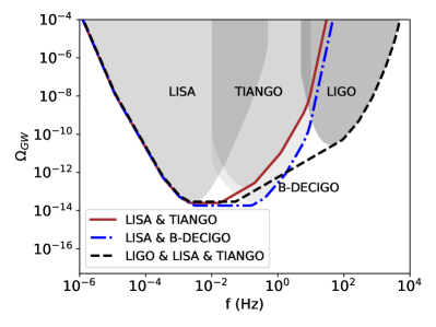
Figure 1 shows the power law sensitivity curves for our three main experiments, given our assumed models, as well as the power law sensitivity for the combination. In the transitional region between LIGO and LISA, the midband experiment TianGo improves sensitivity by several orders of magnitude.
LISA: We use the noise model from [64], which is based on the LISA science requirements document [2]. This assumes a single detector channel333See [68] for a model with a complete set of detector channels.. We are moderately more ambitious by assuming years of observational data in a year mission (thus setting in Eq. 5). The noise budget at high frequencies is dominated by the “optical metrology system” noise and at low frequencies by the “mass acceleration” noise , where and are dimensionless accuracy constants (see also [69, 70]). For arm length, , the shape of the noise curve is
| (6) | ||||
| (7) | ||||
| (8) |
, which relaxes the sensitivity at high frequencies, comes from white noise displacement of the test masses converted into acceleration. The constant is for LISA. For other missions we have assumed it scales linearly with arm length, as it becomes important when frequency is comparable to round-trip laser time.
We combine Eqs. 6-8 with the gravitational wave transfer function to give
| (9) |
and the transfer function is
| (10) |
Here is the length of the satellite arms, is the frequency in Hz, is the speed of light, is the residual acceleration noise and is the position noise. For LISA, we set m, acceleration noise of m s-2 Hz-1/2 and position noise of m Hz-1/2, sensitive to frequencies between Hz and Hz, following Ref. [64].
TianGo: We use the sensitivity curve from Ref. [6]. This can be derived from Eq. 9 by assuming three satellites sensitive to a frequency range of Hz with an arm length of m, acceleration noise of m s-2 Hz-1/2 and position noise m Hz-1/2. The template includes extra noise at Hz due to gravity gradient.
DECIGO: The DECIGO experiment has two components: an initial mission, B-DECIGO, which comprises three drag-free satellites in a geocentric orbit with an arm length of m, and the full DECIGO mission, which is a constellation of four sets of three drag-free satellites at three different points in a heliocentric orbit. The science target of DECIGO is the detection of the stochastic background from inflation [4, 71, 72]. Here we consider B-DECIGO, as the next generation satellite mission expected to launch in the 2030s. B-DECIGO is expected to be sensitive to frequencies from Hz. The satellites of B-DECIGO have kg test masses with a force noise of and thus acceleration noise of m s-2 Hz-1/2. We assume position noise of m Hz-1/2[72].
AEDGE: AEDGE is an alternative design for a satellite experiment using a detector based on cold atom interferometry, also capable of probing the midband. The sensitivity curves for AEDGE are similar to those for B-DECIGO, although achieved with only two satellites [7]. Our conclusions for B-DECIGO are thus also applicable to AEDGE.
LIGO/VIRGO ground-based detectors: The operational ground-based detector network (including LIGO, VIRGO, KAGRA and LIGO India) in is expected to be well developed. We have conservatively used the presently funded A+ detector [73], although there are proposals [65, 66] for detectors with an order of magnitude better sensitivity. We assume the experiment will obtain years of data and use the public forecast sensitivity curve obtained from the LIGO website444https://dcc.ligo.org/LIGO-T1800042/public.
III Analysis for Benchmark Cosmological Sources
III.1 Cosmological Stochastic Gravitational Wave Backgrounds
We consider two representative cosmological sources of SGWB: cosmic strings and phase transitions. These two new physics scenarios are also being probed by other experimental means. For example, the cosmic microwave background constrains cosmic strings. The Large Hadron Collider and or future collider experiments could probe a Higgs sector capable of producing a strong electroweak (EW) phase transition through precision measurements of Higgs couplings. However, LISA is several orders of magnitude more sensitive to a cosmic string network than current or future microwave background experiments, and can complement related collider searches for an extended Higgs sector [74, 75].
III.1.1 Cosmic Strings
Cosmic strings are one-dimensional topological defects, generically predicted by particle physics theories beyond the standard model. Examples include fundamental strings in superstring theory and vortex-like solutions in field theories with a spontaneously broken symmetry. At macroscopic scales the string properties are characterized by energy per unit length (tension), . The string network forms in the early Universe, composed of a few long strings per horizon volume and copious, unstable string loops (formed upon long string intersections), tracing the background energy by a fraction . For many cosmic string models GW production is usually considered the dominant radiation mode for the oscillating string loops 555Although Ref. [76, 77] argue that particle emission dominates for gauge strings., and yields a SGWB from the accumulation of these decaying string loops. In this work we calculate the SGWB from strings following Ref. [54, 41], which incorporates the simulation results for loop distribution from Ref. [78] and an analytical derivation based on a velocity-dependent one scale (VOS) model 666This loop distribution is widely accepted, but other possibilities are discussed in Refs. [79, 41].
The shape of the SGWB spectrum from strings is sensitive to the cosmic expansion history, and a number of recent papers have explored how an early matter domination or kination period may imprint such a spectrum [29, 54, 80, 33, 29, 32, 34, 35, 81]. For the purpose of this work we consider only the case with a standard cosmology: the post-inflationary Universe is radiation dominated until , when it transitions to matter domination. More complex cosmologies we defer to future work.
The cosmic string SGWB spans a wide range of frequency with a nearly flat plateau towards high . As we specify the cosmic history and the loop distribution, the SGWB signal is parametrized by one parameter, the cosmic string tension . We sample string tensions up to the upper limit from EPTA [82], , which is several orders of magnitude larger than LISA’s detection limit. The excess noise in NANOGrav, if interpreted as a detection of cosmic strings, would imply [43]. The exact upper limit we assume has no effect on our results, as LISA alone is able to detect a cosmic string tension many orders of magnitude lower.
III.1.2 Phase Transitions
A strong first order phase transition (PT) may occur in the early Universe, associated with, for example, electroweak symmetry breaking, generation of a matter-antimatter asymmetry or the formation of dark matter [83]. Notably, with simple extensions to the Higgs sector, in the SM the electroweak symmetry breaking phase transition may be first order, and so trigger electroweak baryogenesis. Such a phase transition can generate a SGWB with a peaky structure [23, 84, 85].
The gravitational wave signal from phase transitions arises from three major effects: collisions between bubbles, long lasting sound waves, and possibly turbulence [23, 10, 86]. Each of these three effects produce a component of gravitational wave spectrum which follow a broken power law, peaking around a frequency which roughly scales as the average bubble size (e.g. [86]). The specific amplitude, power laws and peak location depend on the underlying phase transition model. Recent studies show that the GW component from bubble collisions is generally sub-dominant in many particle physics models, such as the extension of the SM for the electroweak phase transition. It can however be important in special cases such as a classically scale-invariant extension of the SM [87, 88]. The signal from turbulence is currently uncertain, as it may only be derived from numerical simulations, which are challenging in the strongly turbulent regime [89]. We will therefore consider the sound wave component only, neglecting other sources. As described below, we focus on parameter regions where this is likely to be a good approximation (e.g. away from extreme supercooling [87, 40]).
The SGWB spectra from a first order PT is determined by four independent parameters: the bubble wall velocity , the temperature at which the transition occurs, the strength of the transition , and the duration of the transition (which we refer to as hereafter). For any given particle physics model , and can be computed from the field Lagrangian, although requires detailed simulation. As our focus is on detectability using a midband experiment we do not choose a specific particle physics model and instead marginalise over these phenomenological parameters.
The emitted gravitational wave spectrum may be computed from these parameters using the formulae derived in [90, 86, 91, 88]. For a phase transition at temperature , with Hubble expansion rate and bubble size at the percolation time, we have777Ref. [86] uses max, where is the sound speed instead of , but see [90, 91, 92].
| (11) |
The gravitational wave spectrum peaks at a frequency proportional to , which today becomes
| (12) |
is the number of degrees of freedom at the phase transition which for GeV is , assuming particle content as in the SM.
The gravitational wave spectrum today is [90, 64, 88]:
| (13) |
The normalisation comes from fitting to the numerical simulations of Ref. [90].888An erratum was issued for their eq. 39. We use the corrected equation. However, at the time of writing the correction has not propagated to the equivalent equation (eq. 29) of Ref. [86], with which we disagree by a factor of . Here subscript denotes the present day and subscript denotes the time of the phase transition. evolves into and is given by
| (14) |
is the reduced Hubble parameter, which we assume to be in agreement with Planck [93]. We neglect for simplicity the possibility of an early matter dominated phase induced by a very strong phase transition [94]. The shape function is chosen to fit numerical simulations [95, 83]:
| (15) |
The numerical factor Eq. 13 comes from . This shape function overestimates power at small and underestimates it at large . Its domain of validity is , [88]. We are particularly interested in this regime, as it includes the upper limit on for well-constrained phase transition energies. The factor is numerically determined [90]. is the kinetic energy fraction in the fluid, given by
| (16) | ||||
| (17) |
As shown by [96, 91] when the phase transition is slow the gravitational wave amplitude decays by a factor proportional to the optical depth, due to shock formation [97]
| (18) |
so that Eq. 13 is multiplied by when , which is the generic case as noted by Ref. [96].999We define following Ref. [94], but older models, omit the factor of [86]. Thus when , the final equation is
| (19) |
Eq. 19 applies in practice to all our phase transition predictions.
To summarize, this model includes four free parameters. First, the strength of the phase transition, , which controls the amplitude of the gravitational wave signal. Second, , the energy density of the phase transition which controls the frequency of the emitted gravitational waves. Third, the speed of the phase transition, . Finally, the speed of the bubbles, . As occurs only in Eq. 11, it is observationally degenerate with . We therefore fix , a regime where the equations above are accurate. For any given particle physics model for the phase transition, correlates with (e.g. [96]), and is observationally degenerate with a combination of and . For the purposes of our parameter constraints we fix as a fiducial value for which the above equations are valid. We have confirmed explicitly by running dedicated chains that varying produces a three-way parameter degeneracy. We will therefore vary only and in our analysis.
We scan over the range of GeV, the region most relevant for observation with a midband experiment. This includes the GeV energy range generally expected for the electroweak phase transition as well as possible more energetic phase transitions associated with, for example, EW PT in Randall-Sundrum models [98], supersymmetry breaking [99] or a dark sector [24, 26]. We choose to limit in our chains, which generally ensures that the PT can be completed [96].
III.2 Astrophysical Stochastic Gravitational Wave Backgrounds
Gravitational waves have been detected from mergers of compact objects: black holes and neutron stars. These objects also contribute to the SGWB. The unresolved signals that make it up are merger events which are too far away to be detectable, and the early inspiral phase of ultimately observable mergers. The latter emit weakly at low frequencies and thus may last much longer at low frequencies than the mission time of LISA. Coalescing compact objects emit GWs with a spectral energy density , where is the frequency in the source frame. The background energy density is then
| (20) |
Here kg m-3 is the critical density, is the frequency in the observed frame, is the Hubble expansion rate and is the merger rate in Gpc-3 yr-1. For all astrophysical backgrounds we integrate redshift from to , approximately the time of formation of the earliest black hole binaries. We have checked that our results are insensitive to the upper redshift limit.
In the below Section, we discuss a variety of astrophysical SGWB sources. The most important are: the unresolved inspiral phases of the already detected LIGO mergers, which we call Stellar Mass Binary Black Holes (StMBBH), mergers from putative intermediate mass ratio inspirals (IMRIs), and, in the LISA band, extreme mass ratio inspirals (EMRIs). We discuss, and conclude to be subdominant, SGWB signals from supermassive black holes, white dwarf mergers and type 1a supernovae. The SGWB from StMBBH and IMRI can be approximated as a power law with index . The shape of the EMRI SGWB is more complex, but can be approximated by a power law with index for Hz. These astrophysical sources are summarized in Figure 2.
III.2.1 Stellar Mass Black Hole Binary Mergers
Mergers detected in the LIGO band emit GWs at lower frequencies during their inspiral phase [100]. We model the signal from these stellar mass binary black hole (StMBBH) mergers following [101, 102]. We neglect neutron star mergers as they are subdominant and degenerate with the overall merger rate, which we marginalize over. By allowing the merger rate to vary we include possible signals from as-yet undetected sources such as primordial black holes [103]. We note that there is still considerable uncertainty in even the shape of the mass function of binary black hole mergers, and that future LIGO merger data may still shift the preferred power law indices [104]. However, the power law index of the SGWB at lower frequencies is dominated by the emission in the inspiral phase and is actually relatively well-characterised, at least compared to other potential SGWB sources.
We compute using separate templates for the merger and inspiral phases from [105]. For the inspiral phase
| (21) |
and are the masses of the two merging objects and is the gravitational constant. During the inspiral phase the emission varies over a wide frequency range. For the merger phase
| (22) |
is the GW frequency at merger in the source frame:
| (23) |
We neglect the subdominant signal from ringdown, and so set for , the source frame ringdown frequency:
| (24) |
Thus , the total energy emitted as a function of frequency, is the sum of the signals from merger and inspiral, integrated over the mass distributions, and .
In the LISA band the stochastic signal is dominated by the low-frequency inspiral phases, while the merger phase is important only in the LIGO band. We assume mergers occur for masses . has a power law mass distribution and is uniformly distributed. We note that the best fit to the latest LIGO data is a slightly steeper power law with an index of and a separate Gaussian peak at [104], which differs moderately from our model. However, our assumed model is only moderately disfavoured at present.
We assume that the merger rate evolves with redshift following an empirical fit to the star formation rate:
| (25) |
We take , , and we define a normalizing constant to specify the rate at , which we leave as a free parameter in our Markov chains. The shape of and the values of and are currently uncertain. However, in the midband region the signal is dominated by the early inspiral phase of relatively low redshift binaries, so we found that for reasonable values of these parameters they were degenerate with the total merger rate. For similar reasons we have not attempted to remove the contribution for merger events resolved by LIGO, which is also degenerate with the overall merger rate.
III.2.2 Extreme Mass Ratio Inspirals
LISA will be sensitive to extreme mass ratio inspirals (EMRIs), mergers between stellar mass and supermassive black holes (SuMBH) [106, 107, 108]. The merger frequency of these objects is approximately
| (26) |
The non-detection of a black hole in M33 [109] suggests that a reasonable guess for a lower limit on the SuMBH mass is , while cosmological simulations use a seed mass around . The EMRI signal thus lies within the LISA band, and would not be detected by a midband experiment. A typical EMRI signal lasts year and includes up to orbits [107]. A fiducial merger rate is Gpc-3 year-1, or LISA detections year-1 [110]. Although these signals are faint, the mock LISA data challenge [111] demonstrated that they are detectable in the datastream due to the high number of orbits.
Modeling the overall signal from EMRIs is complex, as they have a large range of possible parameters, including both black hole masses, eccentricity and black hole spin. We use the EMRI population model from Ref. [112], based on the fiducial population model (M1) of Ref. [107], with detected sources removed. We calculate using
| (27) |
where is the EMRI SGWB characteristic strain. When making forecasts, we leave the overall rate of EMRI mergers as a free parameter to model uncertainty in the EMRI population [113, 107].
III.2.3 Supermassive Black Holes
LISA will also be sensitive to mergers between two SuMBH of masses . We do not consider the stochastic background from these objects as LISA is sensitive enough to detect essentially all such mergers for . At higher redshifts the expected number of supermassive black hole mergers is reduced exponentially, following the number density of halos and the expected timescale for SuMBH formation. SuMBH with , when they occur, would merge in a timescale too short to be resolved from LISA’s data stream [114]. As these objects are rare, brief, transients, they are better treated as glitches rather than a SGWB and so we do not include them.
III.2.4 Intermediate Mass Ratio Inspirals
Between stellar mass and supermassive black hole populations lies a hypothetical population of intermediate mass black holes (IMBH) with [106, e.g ]. The best candidate for their production is dense star clusters which may produce a runaway merger [115, 116]. Only one IMBH has yet been observed, indirectly as the outcome of GW190521 [117], although some may be accessible with LIGO [118].
We can postulate Intermediate Mass Ratio Inspirals (IMRIs) with a mass ratio of , resulting from the merger of stellar mass black holes and IMBHs. Such a merger would be observable by a midband experiment at Hz [119]. Like EMRIs, the merger rate would depend on a variety of uncertain parameters, including the dynamics inside star clusters and the spin distribution of the IMBH.
These mergers would produce a corresponding SGWB. However, the shape of the merger has not yet been computed in the literature. We therefore model the IMRI signal using the same model as we used for stellar mass binary black holes, modifying only the mass distribution of the IMBH and the fiducial merger rate. We assume for the IMBH a uniform mass distribution with a range . Ref. [106] predicted the inspiral phase of IMRIs could be observed by LISA, implying a merger rate of Gpc-3 year-1. We thus choose a fiducial merger rate for our IMRI SGWB model of Gpc-3 year-1.
At this rate the SGWB from IMRIs in the LISA band is similar, but subdominant to, the SGWB from stellar mass binaries merging in the LIGO band. At low frequencies the shape of the signal is completely degenerate with the lower mass objects, with the degeneracy being broken only by the signal from the merger phase in the midband.
Our modeling of the IMRI SGWB is simplistic and likely to be incorrect in detail. However, we suspect that the broad picture of a SGWB component, moderately subdominant to stellar mass binary black holes, degenerate during inspiral and distinguishable during mergers, is likely to be upheld by more detailed future modeling.
III.2.5 White Dwarf Mergers
LISA is sensitive to gravitational wave emission from white dwarf mergers, weak unresolved instances of which would also produce a stochastic gravitational wave background [120]. However, as the emission from these objects is weak, LISA’s sensitivity is limited to mergers in the Milky Way. The stochastic signal from these objects would thus be highly anisotropic, both in space and in time (due to the earth’s rotation around the Sun). We assume that the stochastic signal can be successfully decomposed using angular harmonics, and all but the isotropic component discarded, effectively allowing the white dwarf background to be neglected [121, 122, 59].
III.2.6 Slowly Rotating Neutron Stars
Non-axisymmetric neutron stars are expected to produce gravitational waves [123, 124]. These gravitational waves arise from the rotation of a small deviation from spherical symmetry and have a frequency twice the rotational frequency of the neutron star. The stochastic background from this source thus peaks at high frequencies, reaching perhaps at Hz and dropping to by Hz [125, 126], although these amplitude estimates are uncertain. These gravitational waves may thus be marginally detectable by LIGO detectors, but sensitivity is likely to be limited to the Milky Way [127] and can thus be separated from other SGWB sources through their angular harmonics, as with white dwarf mergers.
III.2.7 Type 1a Supernovae
A source of gravitational waves unique to a midband experiment is type 1a supernovae, whose GW signal peaks in the Hz range [128]. There is no inspiral phase to this event, as the supernovae are assumed to originate from white dwarfs reaching the Chandrasekhar mass by accretion. The events are also faint, with a peak energy of erg/Hz in a frequency range of Hz. If we approximate in Eq. 20 as , then we have
| (28) |
For a cosmological type 1a rate of yr-1 Gpc-3 [129], and Hz, this evaluates to , small enough that we can safely neglect it.
Note that this result is physically due to the lack of an inspiral phase. The full GW energy is released in s and thus produces detectable events without contributing significantly to a SGWB.
III.3 Forecast Generation
For our analysis, we first consider signals with fiducial astrophysical SGWB models only. We generate forecasts to show how a midband experiment can improve constraints on cosmogenic SGWB signals. The upper confidence limits on these parameters provides an estimate of the level at which we could rule out the cosmological signal with the provided set of detectors. We then sample a likelihood function which allows for a non-zero cosmic string or phase transition GW signal. To investigate discovery potential, we separately estimate our ability to extract parameters from models containing cosmological SGWB sources, both a phase transition and a cosmic string background.
Our likelihood function is derived from the overall sensitivity curves of each experiment, and is defined similarly to the squared power-law sensitivity of Eq. 5 as
| (29) |
Here is the length of each experiment and is the model prediction for a SGWB signal with frequency and parameters . is the noise spectral density for each experiment, computed using Eq. 9. is the mock data, generated without detector noise101010Detector noise is not necessary to forecast the experimental covariances. using the default parameters of our astrophysical model. This was a stellar mass BH merger rate of Gpc-3 yr-1, an IMBH merger rate of Gpc-3 yr-1 and an EMRI merger rate matching the fiducial choices of Ref. [112]. We perform separate chains where includes a cosmological signal. For cosmic strings we include a SGWB with , and for a phase transition we use GeV and , which peaks at Hz, in the midband region.
The summation denotes a summation over experiments. Since we are interested in the extra constraining power of a midband experiment we compare LISA, LIGO to constraints from chains which also include a midband experiment, either B-DECIGO or TianGo. We thus generated multiple chains using different experiments.
Markov chains were sampled using EMCEE [130], a widely used affine-invariant sampler. We ran the sampler using walkers for samples each. The walkers were initialized at randomly chosen positions in a ball in the middle of parameter space and moved for samples each. These samples were then discarded and the position of the walkers used as the initial positions for the main sampling run. Acceptance fractions after burn-in were .
To summarize our parameters, they were: 1) The overall merger rate of stellar mass black holes. 2) The overall merger rate of intermediate mass ratio black holes. 3) The overall rate of EMRI mergers. Depending on the cosmological model we then had: 4) The cosmic string tension , or 4) the phase transition temperature scale and 5) the phase transition strength .
IV Results
IV.1 Astrophysical SGWB sources
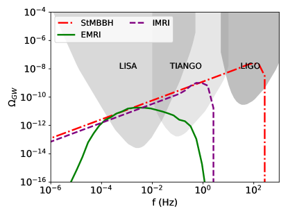
Figure 2 shows example signals from the astrophysical SGWB signals. We show for comparison the PLS for LIGO, LISA and TianGo. Midband experiments improve sensitivity in the region between Hz and Hz. In addition to TianGo, we have run chains with B-DECIGO, which has roughly a factor of two higher sensitivity.
The astrophysical signal from StMBBH and IMRIs is dominated by the inspiral phase until near the peak amplitude. These two astrophysical signals have similar shapes and we have chosen the (uncertain) fiducial merger rate of the IMBH SGWB so that the amplitude of the GW signal is similar to the fiducial StMBBH signal. They are thus extremely degenerate in the LISA and midband frequency channels, although this degeneracy is broken by the high frequency measurements of LIGO and (somewhat) by the signal from the merger phase at Hz. The shape of the EMRI signal differs substantially, as explained in [112]. That the overall amplitude is similar in the LISA band to the fiducial StMBBH merger rate is largely a coincidence and sensitive to our assumptions about how many EMRI mergers are resolvable.
IV.2 Cosmic Strings
IV.2.1 Constraints
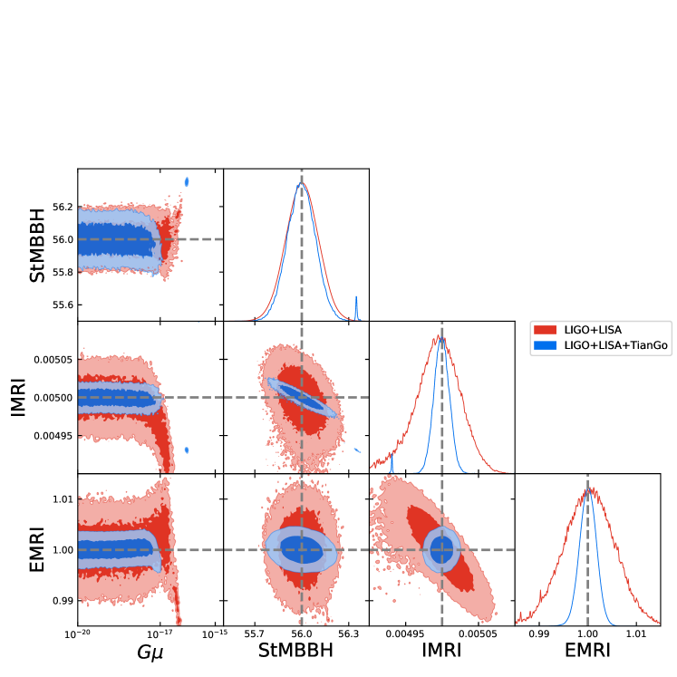
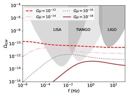
Figure 3 shows the results of our forecast for constraining a cosmic string SGWB based on mock data including astrophysical sources only. We compare the likelihood contours with only LISA and LIGO to those including TianGo. The midband experiment produces a quantitative improvement in the constraints. With only LIGO and LISA, the marginalised upper confidence limit on was , whereas with TianGo it became , an improvement of a factor of . We performed chains with the more sensitive B-DECIGO experiment and found an upper limit of , an improvement of a further factor of .
The improvement in the upper limit on is driven by improved constraints on the SGWB from EMRI and IMRI, which improves following the power law sensitivity of the combined experiments. StMBBH rate constraints do not improve substantially as they are already well constrained by LIGO. Figure 4 explains these results: because the SGWB from cosmic strings is flat between Hz and Hz, LISA dominates the sensitivity if astrophysical sources are neglected. Improvements in constraints with TianGo are thus driven primarily by improved component separation.
Note that, since neither IMRIs nor EMRIs emit at LIGO frequencies, the third generation detectors are unlikely to further improve component separation. However, the raw improvement by a factor of in sensitivity to means that the third generation network may be able to directly detect a cosmic string SGWB with [66].
IV.2.2 Discovery Potential
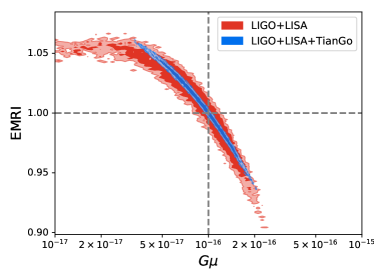
To further assess discovery potential, we ran chains where the simulated data include a cosmic string SGWB with , near the edge of the amplitude detectable with LISA. As expected, without a midband experiment, the string signal was detected at low confidence. Figure 5 shows our results. A strong curving degeneracy emerged between the amplitude of the EMRI SGWB signal and the cosmic string signal: in the presence of a cosmological signal, LISA alone was unable to correctly separate astrophysical and cosmological components. The degeneracy ran between , and , while the EMRI merger rate runs between and the fiducial rate. Since we have probably underestimated the uncertainty in the EMRI SGWB by assuming the fiducial model of [112], this suggests that LISA will struggle to perform component separation for these low string tensions. The addition of the extra information from a midband experiment resolved this issue. Cosmic strings were separated from the EMRI SGWB with a % confidence interval on the tension of for TianGo. For B-DECIGO the interval was slightly narrower, .
IV.3 Phase Transitions
IV.3.1 Constraints
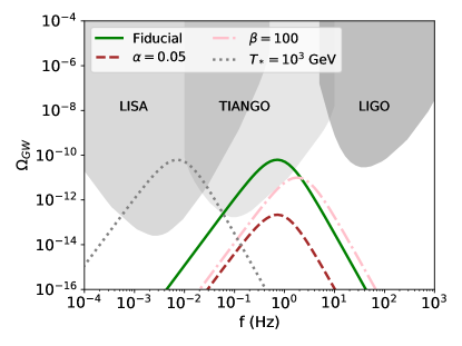
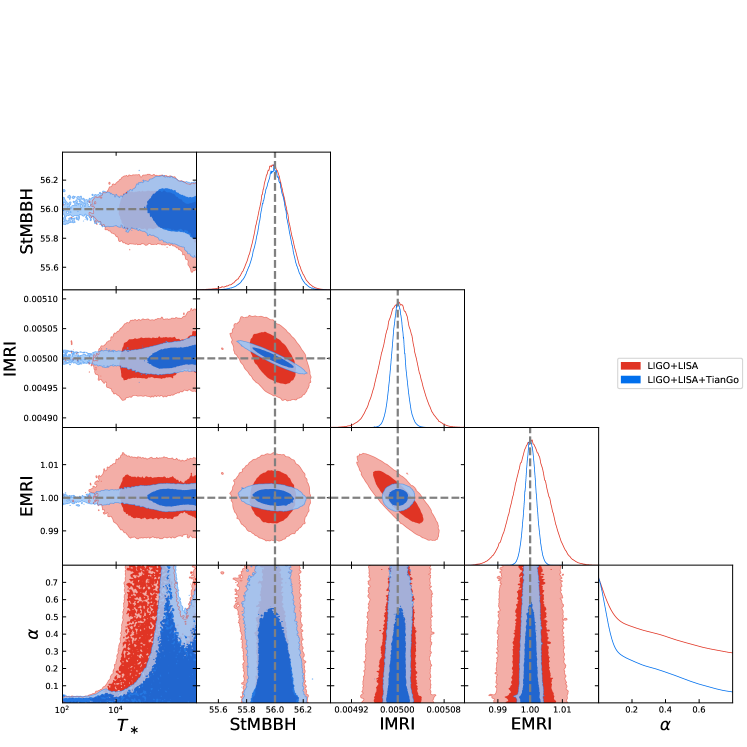
Figure 6 shows the expected SGWB signal from a variety of phase transitions. This SGWB signal is sharply peaked, at a frequency depending on the energy scale and an amplitude directly proportional to the strength of the transition. For our fiducial choice of , transitions peak in the midband region with a temperature (or energy scale) at GeV. Transitions around the electroweak energy scale at GeV peak in the LISA band. Finally, strong phase transitions with GeV peak in the LIGO band, although these are only detectable for . A future third generation network with a sensitivity improvement of would further close this energy gap and improve constraints on phase transitions in this energy band to . For completeness, we also show the effect of increasing . This increases the peak frequency by decreasing the effective bubble size as well as decreasing the amplitude of the SGWB.
Figure 6 thus suggests that there is a region of parameter space where the midband experiment will sharply constrain the presence of a phase transition, and a region of parameter space where the signal peaks at lower energies, within the LISA frequency range. This is confirmed by Figure 7, where we shows constraints on the phase transition parameters from our Markov chains, including only astrophysical SGWBs. Again we show LISA and LIGO only, followed by the results also including TianGo. The midband experiment does not improve constraints for phase transitions with GeV, where detectability is dominated by LIGO. For transitions with GeV, LISA dominates the constraints, and the midband has little effect.
For phase transitions with GeV, the midband experiment substantially improves constraints, as these transitions peak in a frequency band where only the midband experiment has sensitivity. The TianGo experiment leaves a small window around GeV where the presence of a phase transition is not well constrained. Our B-DECIGO chains show that the more sensitive experiment also closes this window.
IV.3.2 Discovery Potential
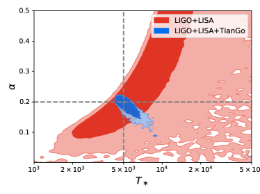
To assess discovery potential, we have run chains where the mock signal includes a phase transition with a variety of energies. We set . We found that, because there is uncertainty on the parameters of the phase transition, there is an energy region where experiments can detect the transition signal, but not estimate its parameters correctly. For example, a transition with GeV and is within the range detectable by LISA. However, because LISA is much less sensitive at higher frequencies, it is not able distinguish a SGWB which peaks within the LISA band and then diminishes in the midband from one which peaks in the midband. Thus it is difficult for LISA to estimate the parameters of the phase transition for signals near the edge of its sensitivity as it cannot measure both sides of the peak in the SGWB. Figure 8 shows our results for this parameter choice. With the combination of LISA and LIGO111111LIGO does not probe these scales, but is necessary to constrain the astrophysical signal from StMBBH., we can only constrain that GeV and , with a range of possible signals at higher and tracing the edge of the LISA PLS curve. The TianGo midband experiment provides extra frequency coverage and measures between and GeV, with . At lower energies in the expected region for an electroweak phase transition, a cosmological signal with GeV had parameters which were fairly well localised by LISA alone, which found at .
We further examined the effect of the gap TianGo leaves at GeV on our constraints. We found that a signal with GeV can be detected with a combination of LISA, LIGO and TianGo, producing confidence intervals of GeV and , with slightly smaller parameter ranges for B-DECIGO. However, a higher energy transition with GeV was only reliably separable with B-DECIGO, as TianGo was unable to localise the transition energy away from the poorly measured GeV region. The more sensitive B-DECIGO or AEDGE is thus preferred for the most robust phase transition measurement.
IV.4 Discussion: Uncertainties in the Astrophysical SGWB Models
Here we assess the likely uncertainty in our conclusions due to our modeling choices for astrophysical SGWB sources. The amplitude of the StMBBH background is currently uncertain by a factor of two, while the EMRI background is uncertain at an order of magnitude level. For the SGWB from IMRI mergers, even the shape is uncertain, although the power law index of the SGWB is likely to be between that of the EMRI and StMBBH backgrounds. Our quantitative forecast limits with B-DECIGO/AEDGE ( and strong constraints on phase transitions in the GeV range) thus represent an estimate. Qualitatively, however, the model we have built includes a separate astrophysical SGWB source in each frequency band: LIGO, LISA and the midband. As long as the IMRI SGWB is close to a power law with index and the EMRI SGWB close to our assumed shape, our conclusion that a midband experiment improves component separation will be valid. Over the next decade a great deal of new data will become available. In particular, once LISA and TianGo begin taking data they should detect EMRI and IMRI mergers, and thus will better constrain the power law index of the SGWB.
V Conclusions
We have examined the ability of a future midband gravitational wave experiment to improve detection prospects for cosmological SGWB signals, when combined with the existing LISA and LIGO detectors. We propose a combined power law sensitivity (CPLS) curve as a simple way to quantify the sensitivity to SGWB of detectors covering multiple frequency bands. The CPLS shows that the midband significantly improves sensitivity to in the transitional frequency region between LIGO and LISA.
We then conducted a dedicated analysis of the potential of a midband experiment to improve prospects for probing a cosmogenic SGWB signal in the presence of a variety of realistic astrophysical signals from black hole mergers. We consider phase transitions and cosmic string SGWB templates, and either TianGo or B-DECIGO as prototypical midband experiments. Our results for B-DECIGO are also valid for AEDGE, which has a similar sensitivity curve.
We find that combining a midband with existing detectors substantially improves constraints on the cosmic string tension. Upper limits on strengthen by a factor of with TianGo and with B-DECIGO or AEDGE. We showed that the addition of an extra frequency channel improves component separation for cosmic string signals. We considered a signal near the lower bound accessible to LISA, , and showed that a midband experiment was necessary for the network to distinguish a cosmic string SGWB from the signal due to extreme mass ratio inspirals.
The phase transition energy scale sets the peak frequency of its SGWB signal. The midband experiment is extremely powerful for understanding phase transitions which peak within its observational frequency band. For our fiducial model choices, it severely constrains the strength of a phase transition in the energy scale GeV. With LISA alone, a phase transition in this energy range is not meaningfully constrained, allowing a phase transition strength . TianGo can strongly constrain GeV to . It does, however, leave an energy gap around GeV which requires the more sensitive B-DECIGO or AEDGE to fully close. We show that a midband experiment allows improved parameter measurement in the presence of phase transitions at lower energies, by ruling out the possibility that the signal comes from a strong phase transition in the GeV range. Note that our analysis fixed some observationally degenerate phase transition parameters. By varying these parameters, we could choose plausible parameters for electroweak phase transition models for which the midband experiment would be critical for measurement of the GW signal.
For a transition at the upper end of the electroweak energy range with GeV and , LISA and LIGO alone show an excess distinguishable from the astrophysical model at about . However, with the addition of TianGo to the network, it is possible to measure and with precision and confidently distinguish them from an astrophysical signal. The midband experiment thus allows the combined detector network to measure the properties of a phase transition, while LISA alone will only show that it exists. For measuring the properties of a phase transition at a few TeV, B-DECIGO or AEDGE provides additional power by completely closing the frequency gap between LISA and LIGO. A third generation ground based detector network would further improve constraints at higher energies.
Our approach can be applied to other cosmological SGWB sources and other proposed GW detectors such as MAGIS [131] or BBO [132]. We demonstrated the significant impact of a potential midband GW experiment in boosting detection prospects for a cosmological SGWB. Our modeling code and chains are available at: https://github.com/sbird/grav_midband. Our results can be further generalized to showcase the advantages for probing new physics obtainable by invigorating a well-coordinated multiple frequency band GW program. This could include not just detectors covering LIGO, LISA and midband frequencies but also other frequency channels. For example, the - nano Hz range is accessible by pulsar timing arrays [133, 42] and milli - Hz by Ares [134].
Acknowledgments
Acknowledgements.
SB was supported by NSF grant AST-1817256 and would like to thank his wife, Priya Bird. YC is supported in part by the US Department of Energy under award number DE-SC0008541, and thanks the Kavli Institute for Theoretical Physics (supported by the National Science Foundation under Grant No. NSF PHY-1748958) for support and hospitality while the work was being completed. We thank Mark Hindmarsh, Marek Lewicki and David Weir for helpful discussions and Chia-Feng Chiang for calculating the early time radiation density.References
- Abbott et al. [2016] B. P. Abbott, R. Abbott, T. D. Abbott, M. R. Abernathy, LIGO Scientific Collaboration, and Virgo Collaboration, Observation of Gravitational Waves from a Binary Black Hole Merger, Phys. Rev. Lett. 116, 061102 (2016), arXiv:1602.03837 [gr-qc] .
- [2] The LISA Collaboration, LISA Science Requirements Document, https://www.elisascience.org/files/publications/LISA_L3_20170120.pdf.
- Abbott et al. [2009] B. P. Abbott et al. (VIRGO, LIGO Scientific), An Upper Limit on the Stochastic Gravitational-Wave Background of Cosmological Origin, Nature 460, 990 (2009), arXiv:0910.5772 [astro-ph.CO] .
- Kawamura et al. [2011] S. Kawamura et al., The Japanese space gravitational wave antenna: DECIGO, Classical and Quantum Gravity 28, 094011 (2011).
- Luo et al. [2016] J. Luo et al., TianQin: a space-borne gravitational wave detector, Classical and Quantum Gravity 33, 035010 (2016), arXiv:1512.02076 [astro-ph.IM] .
- Kuns et al. [2020] K. A. Kuns, H. Yu, Y. Chen, and R. X. Adhikari, Astrophysics and cosmology with a decihertz gravitational-wave detector: TianGO, Phys. Rev. D 102, 043001 (2020), arXiv:1908.06004 [gr-qc] .
- El-Neaj et al. [2020] Y. A. El-Neaj et al. (AEDGE), AEDGE: Atomic Experiment for Dark Matter and Gravity Exploration in Space, EPJ Quant. Technol. 7, 6 (2020), arXiv:1908.00802 [gr-qc] .
- Graham et al. [2017] P. W. Graham, J. M. Hogan, M. A. Kasevich, S. Rajendran, and R. W. Romani (MAGIS), Mid-band gravitational wave detection with precision atomic sensors, (2017), arXiv:1711.02225 [astro-ph.IM] .
- Graham et al. [2016] P. W. Graham, J. M. Hogan, M. A. Kasevich, and S. Rajendran, Resonant mode for gravitational wave detectors based on atom interferometry, Phys. Rev. D94, 104022 (2016), arXiv:1606.01860 [physics.atom-ph] .
- Caprini and Figueroa [2018] C. Caprini and D. G. Figueroa, Cosmological backgrounds of gravitational waves, Classical and Quantum Gravity 35, 163001 (2018), arXiv:1801.04268 [astro-ph.CO] .
- Vilenkin [1981] A. Vilenkin, Gravitational radiation from cosmic strings, Phys. Lett. 107B, 47 (1981).
- Turok [1984] N. Turok, Grand Unified Strings and Galaxy Formation, Nucl. Phys. B242, 520 (1984).
- Vachaspati and Vilenkin [1985] T. Vachaspati and A. Vilenkin, Gravitational Radiation from Cosmic Strings, Phys. Rev. D31, 3052 (1985).
- Burden [1985] C. J. Burden, Gravitational Radiation From a Particular Class of Cosmic Strings, Phys. Lett. 164B, 277 (1985).
- Olum and Blanco-Pillado [2000] K. D. Olum and J. J. Blanco-Pillado, Radiation from cosmic string standing waves, Phys. Rev. Lett. 84, 4288 (2000), arXiv:astro-ph/9910354 [astro-ph] .
- Moore et al. [2001] J. N. Moore, E. P. S. Shellard, and C. J. A. P. Martins, On the evolution of Abelian-Higgs string networks, Phys. Rev. D65, 023503 (2001), arXiv:hep-ph/0107171 [hep-ph] .
- Nielsen and Olesen [1973] H. B. Nielsen and P. Olesen, Vortex Line Models for Dual Strings, Nucl. Phys. B61, 45 (1973), [,302(1973)].
- Kibble [1976] T. W. B. Kibble, Topology of Cosmic Domains and Strings, J. Phys. A9, 1387 (1976).
- Jackson et al. [2005] M. G. Jackson, N. T. Jones, and J. Polchinski, Collisions of cosmic F and D-strings, JHEP 10, 013, arXiv:hep-th/0405229 [hep-th] .
- Tye et al. [2005] S. H. H. Tye, I. Wasserman, and M. Wyman, Scaling of multi-tension cosmic superstring networks, Phys. Rev. D71, 103508 (2005), [Erratum: Phys. Rev.D71,129906(2005)], arXiv:astro-ph/0503506 [astro-ph] .
- Dubath et al. [2008] F. Dubath, J. Polchinski, and J. V. Rocha, Cosmic String Loops, Large and Small, Phys. Rev. D77, 123528 (2008), arXiv:0711.0994 [astro-ph] .
- Figueroa et al. [2020] D. G. Figueroa, M. Hindmarsh, J. Lizarraga, and J. Urrestilla, Irreducible background of gravitational waves from a cosmic defect network: update and comparison of numerical techniques, Phys. Rev. D 102, 103516 (2020), arXiv:2007.03337 [astro-ph.CO] .
- Caprini et al. [2009] C. Caprini, R. Durrer, T. Konstandin, and G. Servant, General Properties of the Gravitational Wave Spectrum from Phase Transitions, Phys. Rev. D79, 083519 (2009), arXiv:0901.1661 [astro-ph.CO] .
- Schwaller [2015] P. Schwaller, Gravitational Waves from a Dark Phase Transition, Phys. Rev. Lett. 115, 181101 (2015), arXiv:1504.07263 [hep-ph] .
- Helmboldt et al. [2019] A. J. Helmboldt, J. Kubo, and S. van der Woude, Observational prospects for gravitational waves from hidden or dark chiral phase transitions, Phys. Rev. D 100, 055025 (2019), arXiv:1904.07891 [hep-ph] .
- Hall et al. [2020] E. Hall, T. Konstandin, R. McGehee, H. Murayama, and G. Servant, Baryogenesis From a Dark First-Order Phase Transition, JHEP 04, 042, arXiv:1910.08068 [hep-ph] .
- Cohen et al. [1991] A. G. Cohen, D. B. Kaplan, and A. E. Nelson, Baryogenesis at the weak phase transition, Nucl. Phys. B349, 727 (1991).
- Anderson and Hall [1992] G. W. Anderson and L. J. Hall, The Electroweak phase transition and baryogenesis, Phys. Rev. D45, 2685 (1992).
- Cui et al. [2018] Y. Cui, M. Lewicki, D. E. Morrissey, and J. D. Wells, Cosmic Archaeology with Gravitational Waves from Cosmic Strings, Phys. Rev. D97, 123505 (2018), arXiv:1711.03104 [hep-ph] .
- Caldwell et al. [2019] R. R. Caldwell, T. L. Smith, and D. G. Walker, Using a Primordial Gravitational Wave Background to Illuminate New Physics, Phys. Rev. D 100, 043513 (2019), arXiv:1812.07577 [astro-ph.CO] .
- Cui et al. [2019] Y. Cui, M. Lewicki, D. E. Morrissey, and J. D. Wells, Probing the pre-BBN universe with gravitational waves from cosmic strings, Journal of High Energy Physics 2019, 81 (2019), arXiv:1808.08968 [hep-ph] .
- Cui et al. [2020] Y. Cui, M. Lewicki, and D. E. Morrissey, Gravitational Wave Bursts as Harbingers of Cosmic Strings Diluted by Inflation, Phys. Rev. Lett. 125, 211302 (2020), arXiv:1912.08832 [hep-ph] .
- Chang and Cui [2020] C.-F. Chang and Y. Cui, Stochastic Gravitational Wave Background from Global Cosmic Strings, Phys. Dark Univ. 29, 100604 (2020), arXiv:1910.04781 [hep-ph] .
- Dror et al. [2020] J. A. Dror, T. Hiramatsu, K. Kohri, H. Murayama, and G. White, Testing the Seesaw Mechanism and Leptogenesis with Gravitational Waves, Phys. Rev. Lett. 124, 041804 (2020), arXiv:1908.03227 [hep-ph] .
- Buchmuller et al. [2020a] W. Buchmuller, V. Domcke, H. Murayama, and K. Schmitz, Probing the scale of grand unification with gravitational waves, Phys. Lett. B 809, 135764 (2020a), arXiv:1912.03695 [hep-ph] .
- Gouttenoire et al. [2020a] Y. Gouttenoire, G. Servant, and P. Simakachorn, Beyond the Standard Models with Cosmic Strings, JCAP 07, 032, arXiv:1912.02569 [hep-ph] .
- Gouttenoire et al. [2020b] Y. Gouttenoire, G. Servant, and P. Simakachorn, BSM with Cosmic Strings: Heavy, up to EeV mass, Unstable Particles, JCAP 07, 016, arXiv:1912.03245 [hep-ph] .
- Dev et al. [2019] P. B. Dev, F. Ferrer, Y. Zhang, and Y. Zhang, Gravitational Waves from First-Order Phase Transition in a Simple Axion-Like Particle Model, JCAP 11, 006, arXiv:1905.00891 [hep-ph] .
- Abbott et al. [2018] B. P. Abbott et al. (LIGO Scientific, Virgo), Constraints on cosmic strings using data from the first Advanced LIGO observing run, Phys. Rev. D97, 102002 (2018), arXiv:1712.01168 [gr-qc] .
- Caprini et al. [2020] C. Caprini et al., Detecting gravitational waves from cosmological phase transitions with LISA: an update, JCAP 2003, 024, arXiv:1910.13125 [astro-ph.CO] .
- Auclair et al. [2020] P. Auclair et al., Probing the gravitational wave background from cosmic strings with LISA, JCAP 2004, 034, arXiv:1909.00819 [astro-ph.CO] .
- Arzoumanian et al. [2020] Z. Arzoumanian et al. (NANOGrav), The NANOGrav 12.5 yr Data Set: Search for an Isotropic Stochastic Gravitational-wave Background, Astrophys. J. Lett. 905, L34 (2020), arXiv:2009.04496 [astro-ph.HE] .
- Ellis and Lewicki [2021] J. Ellis and M. Lewicki, Cosmic String Interpretation of NANOGrav Pulsar Timing Data, Phys. Rev. Lett. 126, 041304 (2021), arXiv:2009.06555 [astro-ph.CO] .
- Addazi et al. [2020] A. Addazi, Y.-F. Cai, Q. Gan, A. Marciano, and K. Zeng, NANOGrav results and Dark First Order Phase Transitions, (2020), arXiv:2009.10327 [hep-ph] .
- Ratzinger and Schwaller [2021] W. Ratzinger and P. Schwaller, Whispers from the dark side: Confronting light new physics with NANOGrav data, SciPost Phys. 10, 047 (2021), arXiv:2009.11875 [astro-ph.CO] .
- Blasi et al. [2021] S. Blasi, V. Brdar, and K. Schmitz, Has NANOGrav found first evidence for cosmic strings?, Phys. Rev. Lett. 126, 041305 (2021), arXiv:2009.06607 [astro-ph.CO] .
- Buchmuller et al. [2020b] W. Buchmuller, V. Domcke, and K. Schmitz, From NANOGrav to LIGO with metastable cosmic strings, Phys. Lett. B 811, 135914 (2020b), arXiv:2009.10649 [astro-ph.CO] .
- Samanta and Datta [2020] R. Samanta and S. Datta, Gravitational wave complementarity and impact of NANOGrav data on gravitational leptogenesis: cosmic strings, (2020), arXiv:2009.13452 [hep-ph] .
- Nakai et al. [2021] Y. Nakai, M. Suzuki, F. Takahashi, and M. Yamada, Gravitational Waves and Dark Radiation from Dark Phase Transition: Connecting NANOGrav Pulsar Timing Data and Hubble Tension, Phys. Lett. B 816, 136238 (2021), arXiv:2009.09754 [astro-ph.CO] .
- Neronov et al. [2021] A. Neronov, A. Roper Pol, C. Caprini, and D. Semikoz, NANOGrav signal from magnetohydrodynamic turbulence at the QCD phase transition in the early Universe, Phys. Rev. D 103, L041302 (2021), arXiv:2009.14174 [astro-ph.CO] .
- Smith and Thrane [2018] R. Smith and E. Thrane, Optimal Search for an Astrophysical Gravitational-Wave Background, Phys. Rev. X 8, 021019 (2018), arXiv:1712.00688 [gr-qc] .
- Bartolo et al. [2018] N. Bartolo, V. Domcke, D. G. Figueroa, J. García-Bellido, M. Peloso, M. Pieroni, A. Ricciardone, M. Sakellariadou, L. Sorbo, and G. Tasinato, Probing non-Gaussian Stochastic Gravitational Wave Backgrounds with LISA, JCAP 11, 034, arXiv:1806.02819 [astro-ph.CO] .
- Ginat et al. [2020] Y. B. Ginat, V. Desjacques, R. Reischke, and H. B. Perets, Probability distribution of astrophysical gravitational-wave background fluctuations, Phys. Rev. D 102, 083501 (2020), arXiv:1910.04587 [astro-ph.CO] .
- Cui et al. [2019] Y. Cui, M. Lewicki, D. E. Morrissey, and J. D. Wells, Probing the pre-BBN universe with gravitational waves from cosmic strings, JHEP 01, 081, arXiv:1808.08968 [hep-ph] .
- Romano and Cornish [2017] J. D. Romano and N. J. Cornish, Detection methods for stochastic gravitational-wave backgrounds: a unified treatment, Living Reviews in Relativity 20, 2 (2017), arXiv:1608.06889 [gr-qc] .
- Romano [2019] J. D. Romano, Searches for stochastic gravitational-wave backgrounds, arXiv e-prints (2019), arXiv:1909.00269 [gr-qc] .
- Cutler and Harms [2006] C. Cutler and J. Harms, Big Bang Observer and the neutron-star-binary subtraction problem, Phys. Rev. D 73, 042001 (2006), arXiv:gr-qc/0511092 [gr-qc] .
- Pan and Yang [2020] Z. Pan and H. Yang, Probing Primordial Stochastic Gravitational Wave Background with Multi-band Astrophysical Foreground Cleaning, Class. Quant. Grav. 37, 195020 (2020), arXiv:1910.09637 [astro-ph.CO] .
- Pieroni and Barausse [2020] M. Pieroni and E. Barausse, Foreground cleaning and template-free stochastic background extraction for LISA, JCAP 2020, 021 (2020), arXiv:2004.01135 [astro-ph.CO] .
- Boileau et al. [2021] G. Boileau, N. Christensen, R. Meyer, and N. J. Cornish, Spectral separation of the stochastic gravitational-wave background for LISA: Observing both cosmological and astrophysical backgrounds, Phys. Rev. D 103, 103529 (2021), arXiv:2011.05055 [gr-qc] .
- Sedda et al. [2020] M. A. Sedda et al., The missing link in gravitational-wave astronomy: discoveries waiting in the decihertz range, Class. Quant. Grav. 37, 215011 (2020), arXiv:1908.11375 [gr-qc] .
- Thrane and Romano [2013] E. Thrane and J. D. Romano, Sensitivity curves for searches for gravitational-wave backgrounds, Phys. Rev. D88, 124032 (2013), arXiv:1310.5300 [astro-ph.IM] .
- Moore et al. [2015] C. J. Moore, R. H. Cole, and C. P. L. Berry, Gravitational-wave sensitivity curves, Classical and Quantum Gravity 32, 015014 (2015), arXiv:1408.0740 [gr-qc] .
- Caprini et al. [2019] C. Caprini, D. G. Figueroa, R. Flauger, G. Nardini, M. Peloso, M. Pieroni, A. Ricciardone, and G. Tasinato, Reconstructing the spectral shape of a stochastic gravitational wave background with LISA, JCAP 11, 017, arXiv:1906.09244 [astro-ph.CO] .
- Reitze et al. [2019] D. Reitze et al., Cosmic Explorer: The U.S. Contribution to Gravitational-Wave Astronomy beyond LIGO, Bull. Am. Astron. Soc. 51, 035 (2019), arXiv:1907.04833 [astro-ph.IM] .
- Maggiore et al. [2020] M. Maggiore et al., Science Case for the Einstein Telescope, JCAP 03, 050, arXiv:1912.02622 [astro-ph.CO] .
- Ruan et al. [2020] W.-H. Ruan, Z.-K. Guo, R.-G. Cai, and Y.-Z. Zhang, Taiji program: Gravitational-wave sources, Int. J. Mod. Phys. A 35, 2050075 (2020), arXiv:1807.09495 [gr-qc] .
- Flauger et al. [2021] R. Flauger, N. Karnesis, G. Nardini, M. Pieroni, A. Ricciardone, and J. Torrado, Improved reconstruction of a stochastic gravitational wave background with LISA, JCAP 01, 059, arXiv:2009.11845 [astro-ph.CO] .
- Larson et al. [2000] S. L. Larson, W. A. Hiscock, and R. W. Hellings, Sensitivity curves for spaceborne gravitational wave interferometers, Phys. Rev. D 62, 062001 (2000), arXiv:gr-qc/9909080 [gr-qc] .
- Cornish and Rubbo [2003] N. J. Cornish and L. J. Rubbo, Publisher’s Note: LISA response function [Phys. Rev. D 67, 022001 (2003)], Phys. Rev. D 67, 029905(E) (2003), arXiv:gr-qc/0209011 [gr-qc] .
- Sato et al. [2017] S. Sato et al., The status of DECIGO, Journal of Physics: Conference Series 840, 012010 (2017).
- Nakamura et al. [2016] T. Nakamura et al., Pre-DECIGO can get the smoking gun to decide the astrophysical or cosmological origin of GW150914-like binary black holes, Progress of Theoretical and Experimental Physics 2016, 093E01 (2016), arXiv:1607.00897 [astro-ph.HE] .
- National Science Foundation [2019] National Science Foundation, Press statement: Upgraded LIGO to search for universe’s most extreme events., https://www.nsf.gov/news/news_summ.jsp?cntn_id=297414 (2019).
- Huang et al. [2016] P. Huang, A. J. Long, and L.-T. Wang, Probing the Electroweak Phase Transition with Higgs Factories and Gravitational Waves, Phys. Rev. D 94, 075008 (2016), arXiv:1608.06619 [hep-ph] .
- Gould et al. [2019] O. Gould, J. Kozaczuk, L. Niemi, M. J. Ramsey-Musolf, T. V. Tenkanen, and D. J. Weir, Nonperturbative analysis of the gravitational waves from a first-order electroweak phase transition, Phys. Rev. D 100, 115024 (2019), arXiv:1903.11604 [hep-ph] .
- Vincent et al. [1998] G. Vincent, N. D. Antunes, and M. Hindmarsh, Numerical simulations of string networks in the Abelian Higgs model, Phys. Rev. Lett. 80, 2277 (1998), arXiv:hep-ph/9708427 [hep-ph] .
- Bevis et al. [2007] N. Bevis, M. Hindmarsh, M. Kunz, and J. Urrestilla, CMB power spectrum contribution from cosmic strings using field-evolution simulations of the Abelian Higgs model, Phys. Rev. D75, 065015 (2007), arXiv:astro-ph/0605018 [astro-ph] .
- Blanco-Pillado et al. [2014] J. J. Blanco-Pillado, K. D. Olum, and B. Shlaer, The number of cosmic string loops, Phys. Rev. D89, 023512 (2014), arXiv:1309.6637 [astro-ph.CO] .
- Ringeval et al. [2007] C. Ringeval, M. Sakellariadou, and F. Bouchet, Cosmological evolution of cosmic string loops, JCAP 0702, 023, arXiv:astro-ph/0511646 [astro-ph] .
- D’Eramo and Schmitz [2019] F. D’Eramo and K. Schmitz, Imprint of a scalar era on the primordial spectrum of gravitational waves, Phys. Rev. Research. 1, 013010 (2019), arXiv:1904.07870 [hep-ph] .
- Blasi et al. [2020] S. Blasi, V. Brdar, and K. Schmitz, Fingerprint of low-scale leptogenesis in the primordial gravitational-wave spectrum, Phys. Rev. Res. 2, 043321 (2020), arXiv:2004.02889 [hep-ph] .
- van Haasteren et al. [2011] R. van Haasteren et al., Placing limits on the stochastic gravitational-wave background using European Pulsar Timing Array data, MNRAS 414, 3117 (2011), arXiv:1103.0576 [astro-ph.CO] .
- Caprini et al. [2016] C. Caprini et al., Science with the space-based interferometer eLISA. II: gravitational waves from cosmological phase transitions, JCAP 2016, 001 (2016), arXiv:1512.06239 [astro-ph.CO] .
- Alanne et al. [2020] T. Alanne, T. Hugle, M. Platscher, and K. Schmitz, A fresh look at the gravitational-wave signal from cosmological phase transitions, Journal of High Energy Physics 2020, 4 (2020), arXiv:1909.11356 [hep-ph] .
- Schmitz [2021] K. Schmitz, New Sensitivity Curves for Gravitational-Wave Signals from Cosmological Phase Transitions, JHEP 01, 097, arXiv:2002.04615 [hep-ph] .
- Caprini et al. [2020] C. Caprini et al., Detecting gravitational waves from cosmological phase transitions with LISA: an update, JCAP 2020, 024 (2020), arXiv:1910.13125 [astro-ph.CO] .
- Ellis et al. [2019] J. Ellis, M. Lewicki, J. M. No, and V. Vaskonen, Gravitational wave energy budget in strongly supercooled phase transitions, JCAP 06, 024, arXiv:1903.09642 [hep-ph] .
- Hindmarsh et al. [2021] M. B. Hindmarsh, M. Lüben, J. Lumma, and M. Pauly, Phase transitions in the early universe, SciPost Phys. Lect. Notes 24, 1 (2021), arXiv:2008.09136 [astro-ph.CO] .
- Cutting et al. [2020] D. Cutting, M. Hindmarsh, and D. J. Weir, Vorticity, Kinetic Energy, and Suppressed Gravitational-Wave Production in Strong First-Order Phase Transitions, Phys. Rev. Lett. 125, 021302 (2020), arXiv:1906.00480 [hep-ph] .
- Hindmarsh et al. [2017] M. Hindmarsh, S. J. Huber, K. Rummukainen, and D. J. Weir, Shape of the acoustic gravitational wave power spectrum from a first order phase transition, Phys. Rev. D 96, 103520 (2017), arXiv:1704.05871 [astro-ph.CO] .
- Guo et al. [2021] H.-K. Guo, K. Sinha, D. Vagie, and G. White, Phase Transitions in an Expanding Universe: Stochastic Gravitational Waves in Standard and Non-Standard Histories, JCAP 01, 001, arXiv:2007.08537 [hep-ph] .
- Weir [2020] D. J. Weir, Ptplot: a tool for exploring the gravitational wave power spectrum from first-order phase transitions (2020).
- Aghanim et al. [2020] N. Aghanim et al. (Planck), Planck 2018 results. VI. Cosmological parameters, Astron. Astrophys. 641, A6 (2020), arXiv:1807.06209 [astro-ph.CO] .
- Ellis et al. [2020] J. Ellis, M. Lewicki, and V. Vaskonen, Updated predictions for gravitational waves produced in a strongly supercooled phase transition, JCAP 11, 020, arXiv:2007.15586 [astro-ph.CO] .
- Hindmarsh et al. [2015] M. Hindmarsh, S. J. Huber, K. Rummukainen, and D. J. Weir, Numerical simulations of acoustically generated gravitational waves at a first order phase transition, Phys. Rev. D 92, 123009 (2015), arXiv:1504.03291 [astro-ph.CO] .
- Ellis et al. [2019] J. Ellis, M. Lewicki, and J. M. No, On the maximal strength of a first-order electroweak phase transition and its gravitational wave signal, JCAP 2019, 003 (2019), arXiv:1809.08242 [hep-ph] .
- Ellis et al. [2020] J. Ellis, M. Lewicki, and J. M. No, Gravitational waves from first-order cosmological phase transitions: lifetime of the sound wave source, JCAP 2020, 050 (2020), arXiv:2003.07360 [hep-ph] .
- Agashe et al. [2021] K. Agashe, P. Du, M. Ekhterachian, S. Kumar, and R. Sundrum, Phase Transitions from the Fifth Dimension, JHEP 02, 051, arXiv:2010.04083 [hep-th] .
- Craig [2009] N. J. Craig, Gravitational Waves from Supersymmetry Breaking, (2009), arXiv:0902.1990 [hep-ph] .
- Finn and Thorne [2000] L. S. Finn and K. S. Thorne, Gravitational waves from a compact star in a circular, inspiral orbit, in the equatorial plane of a massive, spinning black hole, as observed by LISA, Phys. Rev. D 62, 124021 (2000), arXiv:gr-qc/0007074 [gr-qc] .
- Cholis [2017] I. Cholis, On the gravitational wave background from black hole binaries after the first LIGO detections, JCAP 2017, 037 (2017), arXiv:1609.03565 [astro-ph.HE] .
- Abbott et al. [2019] B. P. Abbott et al. (LIGO Scientific, Virgo), Search for the isotropic stochastic background using data from Advanced LIGO’s second observing run, Phys. Rev. D 100, 061101 (2019), arXiv:1903.02886 [gr-qc] .
- Mandic et al. [2016] V. Mandic, S. Bird, and I. Cholis, Stochastic Gravitational-Wave Background due to Primordial Binary Black Hole Mergers, Phys. Rev. Lett. 117, 201102 (2016), arXiv:1608.06699 [astro-ph.CO] .
- Abbott et al. [2020a] R. Abbott et al. (LIGO Scientific, Virgo), Population Properties of Compact Objects from the Second LIGO-Virgo Gravitational-Wave Transient Catalog, (2020a), arXiv:2010.14533 [astro-ph.HE] .
- Ajith et al. [2008] P. Ajith, S. Babak, Y. Chen, M. Hewitson, B. Krishnan, A. Sintes, et al., A Template bank for gravitational waveforms from coalescing binary black holes. I. Non-spinning binaries, Phys. Rev. D 77, 104017 (2008), [Erratum: Phys.Rev.D 79, 129901 (2009)], arXiv:0710.2335 [gr-qc] .
- Amaro-Seoane et al. [2007] P. Amaro-Seoane et al., TOPICAL REVIEW: Intermediate and extreme mass-ratio inspirals—astrophysics, science applications and detection using LISA, Classical and Quantum Gravity 24, R113 (2007), arXiv:astro-ph/0703495 [astro-ph] .
- Babak et al. [2017] S. Babak et al., Science with the space-based interferometer LISA. V. Extreme mass-ratio inspirals, Phys. Rev. D 95, 103012 (2017), arXiv:1703.09722 [gr-qc] .
- Amaro-Seoane [2018a] P. Amaro-Seoane, Relativistic dynamics and extreme mass ratio inspirals, Living Reviews in Relativity 21, 4 (2018a), arXiv:1205.5240 [astro-ph.CO] .
- Gebhardt et al. [2001] K. Gebhardt et al., M33: A Galaxy with No Supermassive Black Hole, AJ 122, 2469 (2001), arXiv:astro-ph/0107135 [astro-ph] .
- Gair et al. [2004] J. R. Gair et al., Event rate estimates for LISA extreme mass ratio capture sources, Classical and Quantum Gravity 21, S1595 (2004), arXiv:gr-qc/0405137 [gr-qc] .
- Babak et al. [2010] S. Babak et al., The Mock LISA Data Challenges: from challenge 3 to challenge 4, Classical and Quantum Gravity 27, 084009 (2010), arXiv:0912.0548 [gr-qc] .
- Bonetti and Sesana [2020] M. Bonetti and A. Sesana, Gravitational wave background from extreme mass ratio inspirals, Phys. Rev. D 102, 103023 (2020), arXiv:2007.14403 [astro-ph.GA] .
- Amaro-Seoane and Preto [2011] P. Amaro-Seoane and M. Preto, The impact of realistic models of mass segregation on the event rate of extreme-mass ratio inspirals and cusp re-growth, Classical and Quantum Gravity 28, 094017 (2011), arXiv:1010.5781 [astro-ph.CO] .
- Salcido et al. [2016] J. Salcido et al., Music from the heavens - gravitational waves from supermassive black hole mergers in the EAGLE simulations, MNRAS 463, 870 (2016), arXiv:1601.06156 [astro-ph.GA] .
- Ebisuzaki et al. [2001] T. Ebisuzaki et al., Missing Link Found? The “Runaway” Path to Supermassive Black Holes, ApJL 562, L19 (2001), arXiv:astro-ph/0106252 [astro-ph] .
- Miller [2005] M. C. Miller, Probing General Relativity with Mergers of Supermassive and Intermediate-Mass Black Holes, Astrophys. J. 618, 426 (2005), arXiv:astro-ph/0409331 [astro-ph] .
- Abbott et al. [2020b] R. Abbott et al. (LIGO Scientific, Virgo), GW190521: A Binary Black Hole Merger with a Total Mass of 150 M, Phys. Rev. Lett. 125, 101102 (2020b), arXiv:2009.01075 [gr-qc] .
- Ezquiaga and Holz [2021] J. M. Ezquiaga and D. E. Holz, Jumping the Gap: Searching for LIGO’s Biggest Black Holes, Astrophys. J. Lett. 909, L23 (2021), arXiv:2006.02211 [astro-ph.HE] .
- Amaro-Seoane [2018b] P. Amaro-Seoane, Detecting intermediate-mass ratio inspirals from the ground and space, Phys. Rev. D 98, 063018 (2018b), arXiv:1807.03824 [astro-ph.HE] .
- Bender and Hils [1997] P. L. Bender and D. Hils, Confusion noise level due to galactic and extragalactic binaries, Classical and Quantum Gravity 14, 1439 (1997).
- Thrane et al. [2009] E. Thrane, S. Ballmer, J. D. Romano, S. Mitra, D. Talukder, S. Bose, and V. Mandic, Probing the anisotropies of a stochastic gravitational-wave background using a network of ground-based laser interferometers, Phys. Rev. D 80, 122002 (2009), arXiv:0910.0858 [astro-ph.IM] .
- Adams and Cornish [2014] M. R. Adams and N. J. Cornish, Detecting a stochastic gravitational wave background in the presence of a galactic foreground and instrument noise, Phys. Rev. D 89, 022001 (2014), arXiv:1307.4116 [gr-qc] .
- Press and Thorne [1972] W. H. Press and K. S. Thorne, Gravitational-wave astronomy, Annual Review of Astronomy and Astrophysics 10, 335 (1972), https://doi.org/10.1146/annurev.aa.10.090172.002003 .
- Riles [2013] K. Riles, Gravitational Waves: Sources, Detectors and Searches, Prog. Part. Nucl. Phys. 68, 1 (2013), arXiv:1209.0667 [hep-ex] .
- Marassi et al. [2011] S. Marassi, R. Ciolfi, R. Schneider, L. Stella, and V. Ferrari, Stochastic background of gravitational waves emitted by magnetars, Mon. Not. Roy. Astron. Soc. 411, 2549 (2011), arXiv:1009.1240 [astro-ph.CO] .
- Rosado [2012] P. A. Rosado, Gravitational wave background from rotating neutron stars, Phys. Rev. D 86, 104007 (2012), arXiv:1206.1330 [gr-qc] .
- Christensen [2019] N. Christensen, Stochastic Gravitational Wave Backgrounds, Rept. Prog. Phys. 82, 016903 (2019), arXiv:1811.08797 [gr-qc] .
- Seitenzahl et al. [2015] I. R. Seitenzahl, M. Herzog, A. J. Ruiter, K. Marquardt, S. T. Ohlmann, and F. K. Röpke, Neutrino and gravitational wave signal of a delayed-detonation model of type Ia supernovae, Phys. Rev. D 92, 124013 (2015), arXiv:1511.02542 [astro-ph.SR] .
- Bonaparte et al. [2013] I. Bonaparte, F. Matteucci, S. Recchi, E. Spitoni, A. Pipino, and V. Grieco, Galactic and cosmic Type Ia supernova (SNIa) rates: is it possible to impose constraints on SNIa progenitors?, MNRAS 435, 2460 (2013), arXiv:1308.0137 [astro-ph.CO] .
- Foreman-Mackey et al. [2013] D. Foreman-Mackey, D. W. Hogg, D. Lang, and J. Goodman, emcee: The MCMC Hammer, PASP 125, 306 (2013), arXiv:1202.3665 [astro-ph.IM] .
- Adamson et al. [2018] P. Adamson et al., PROPOSAL: P-1101 Matter-wave Atomic Gradiometer Interferometric Sensor (MAGIS-100) 10.2172/1605586 (2018).
- Yagi and Seto [2011] K. Yagi and N. Seto, Detector configuration of DECIGO/BBO and identification of cosmological neutron-star binaries, Phys. Rev. D 83, 044011 (2011), [Erratum: Phys.Rev.D 95, 109901 (2017)], arXiv:1101.3940 [astro-ph.CO] .
- Janssen et al. [2015] G. Janssen et al., Gravitational wave astronomy with the SKA, PoS AASKA14, 037 (2015), arXiv:1501.00127 [astro-ph.IM] .
- Sesana et al. [2019] A. Sesana et al., Unveiling the Gravitational Universe at -Hz Frequencies, (2019), arXiv:1908.11391 [astro-ph.IM] .