Effect of magnon decays on parametrically pumped magnons

Abstract

We investigate the influence of magnon decays on the non-equilibrium dynamics of parametrically excited magnons in the magnetic insulator yttrium-iron garnet (YIG). Our investigations are motivated by a recent experiment by Noack et al. [Phys. Status Solidi B 256, 1900121 (2019)] where an enhancement of the spin pumping effect in YIG was observed near the magnetic field strength where magnon decays via confluence of magnons becomes kinematically possible. To explain the experimental findings, we have derived and solved kinetic equations for the non-equilibrium magnon distribution. The effect of magnon decays is taken into account microscopically via collision integrals derived from interaction vertices involving three powers of magnon operators. Our results agree quantitatively with the experimental data.

I Introduction

In a recent experiment Noack19 the parametric excitation of magnons in the magnetic insulator yttrium-iron garnet (YIG) was investigated by coupling an oscillating microwave field into the system and measuring the magnon density via the inverse spin-Hall effectHirsch99 . This effect, which converts a spin current into an electric field perpendicular to the directions of the spin current and the spin polarization, is caused by the relativistic spin-orbit interactions that are also responsible for the direct spin-Hall effectAndo11 . In solids this effect is enhanced due to the strong potential of atomic nuclei Nagaosa08 . In the experimentNoack19 a thin YIG film was exposed to an oscillating magnetic field $\bm{H}(t)={H}_{0}\bm{e}_{z}+H_{1}\cos(\omega_{0}t)\bm{e}_{z}$, where the static part $H_{0}\bm{e}_{z}$ forces the macroscopic magnetization to be aligned along the $z$-axis $\bm{e}_{z}$, while the oscillating part with amplitude $H_{1}\ll H_{0}$ drives the magnons in the sample out of equilibrium. Noack et al. Noack19 observed that the spin-pumping effect was enhanced for certain values of the static field $H_{0}$, and that the magnon density in the stationary non-equilibrium state displayed peaks or dips for those values of $H_{0}$ where magnon decays due to the confluence of two parametrically excited magnons with identical energy and momentum becomes kinematically possible. Recall that magnon decays due to the confluence and the reverse splitting process conserve the total energy and momentum of the magnons involved in these scattering processes Cherepanov93 ; Lvov94 .

In this work we provide a quantitative microscopic explanation for the experimental observations of Ref. [Noack19, ]. It turns out that therefore a proper understanding of magnon damping under non-equilibrium conditions in YIG is crucial. We therefore construct a kinetic theory of pumped magnon gases including microscopically derived collision integrals describing the relevant dissipative effects. While theoretical investigations of pumped magnon gases in magnetic insulators have a long history Suhl57 ; Schloemann60 ; Zakharov70 ; Zakharov74 ; Vinikovetskii79 ; Cherepanov93 ; Araujo74 ; Tsukernik75 ; Lavrinenko81 ; Zvyagin82 ; Zvyagin85 ; Lim88 ; Kalafati89 ; Lvov94 ; Zvyagin07 ; Rezende09 ; Kloss10 ; Safonov13 ; Slobodianiuk17 ; Hahn20 in all works published so far the effect of collisions on the non-equilibrium magnon dynamics was considered only phenomenologically by introducing (by hand) a relaxation rate into the kinetic equations for the magnon distribution functions. Although the relevant microscopic collision integrals have been derived within the Born approximation in Ref. [Vinikovetskii79, ], to our knowledge a microscopic treatment of the effect of magnon collisions on the non-equilibrium dynamics of magnons is still missing in the literature. An alternative method to investigate the dynamics of pumped magnons in YIG is based on the numerical solution of the stochastic non-Markovian Landau-Lifshitz-Gilbert equation with a microscopically derived noise and dissipation kernel Rueckriegel15 . The approach based on kinetic equations adopted here has the advantage that it allows us to identify the experimentally relevant confluent scattering processes directly in the collision integral. Still, the resulting non-linear integro-differential equations are very complicated and can only be solved numerically. Moreover, the derivation of the collision integrals starting from an effective spin Hamiltonian for YIG is a demanding technical problem because the distribution function of the magnon gas in YIG with external pumping has an off-diagonal component so that we have to deal with various types of anomalous cubic interaction vertices. While in principle the collision integrals can be derived diagrammatically using the Keldysh formalismKamenev11 , to keep track of all terms contributing to the collision integrals we have found it more convenient to use an unconventional method developed in Ref. [Fricke97, ] based on a systematic expansion of the collision integrals in terms of connected equal-time correlation functions.

The rest of this article is organized as follows. In Sec. II we introduce the effective Hamiltonian describing pumped magnons in YIG which is the starting point for our investigations. In Sec. III we derive collisionless kinetic equations for the magnon distribution functions in YIG. We also discuss the usual phenomenological strategy of introducing dissipative effects into the collisionless kinetic equations, derive the resulting stationary non-equilibrium distributions for YIG, and show that the experimental results of Noack et al. Noack19 cannot be explained within this approximation. In Sec. IV we derive the collision integrals containing the cubic vertices using an expansion in powers of connected equal-time correlations Fricke97 . Our numerical results for the stationary non-equilibrium solution including the effects of the cubic vertices are presented in Sec. V. Finally, in Sec. VI we summarize our results and present our conclusions. To make this work self-contained we have added three appendices with technical details. In Appendix A we outline the derivation of the Hamiltonian of pumped magnons in YIG following mainly Refs. [Kreisel09, ; Hick10, ]. In Appendix B we review the method of deriving kinetic equations via an expansion in terms of connected equal-time correlations developed by Fricke Fricke97 , and in Appendix C we give the explicit expressions for the relevant collision integrals for YIG obtained with this method.

II Hamiltonian for pumped magnons in YIG

In the experimental setup of Ref. [Noack19, ] a thin stripe of YIG is exposed to an oscillating microwave field in the parallel pumping geometry where the oscillating component of the magnetic field is parallel to its static component. At the energy scales of interest the magnon dynamics can be described by the following time-dependent effective Hamiltonian,Cherepanov93 ; Lvov94 ; Rezende06 ; Rezende09 ; Kreisel09 ; Hick10 ; Kloss10 ; Rueckriegel14

$${\mathcal{H}}(t) = -\frac{1}{2}\sum\limits_{ij}\sum\limits_{\alpha\beta}\left[J_{ij}\delta^{\alpha\beta}+D_{ij}^{\alpha\beta}\right]S_{i}^{\alpha}S_{j}^{\beta}$$ (1)

$$-\left[h_{0}+h_{1}\cos\left(\omega_{0}t\right)\right]\sum\limits_{i}S_{i}^{z},$$

where the indices $i,j$ label the $N$ sites of a cubic lattice and $\alpha,\beta$ denote the three spin components $x,y,z$ of the spin operators $S_{i}^{\alpha}$. The nearest neighbor exchange couplings connecting lattice sites $\bm{r}_{i}$ and $\bm{r}_{j}$ are denoted by $J_{ij}$, while $D_{ij}^{\alpha\beta}$ denotes the matrix elements of the dipolar tensor defined in Eq. (A1) of Appendix A. The last term in Eq. (1) represents the coupling of the spins to a static magnetic field $H_{0}$ and a time-dependent microwave magnetic field $H_{1}$ oscillating with frequency $\omega_{0}$, where $h_{0}=\mu H_{0}$ and $h_{1}=\mu H_{1}$ are the corresponding Zeeman energies. The geometry of the system and our choice of the coordinate system is shown in Fig. 1.

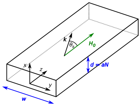
Figure 1: Sketch of a long YIG stripe oriented along the $z$-axis with width $w$ in $y$-direction and thickness $d=aN$ in $x$-direction. Here $a$ is the lattice spacing and $N$ is the number of lattice sites in $x$-direction. In this work we consider wavevectors ${\bm{k}}$ in the $y$-$z$-plane with $\theta_{\bm{k}}$ being the angle between ${\bm{k}}$ and the static magnetic field magnetic field ${\bm{H}}_{0}=H_{0}{\bf e}_{z}$.

The Hamiltonian (1) can be bosonized using the Holstein-Primakoff transformation Holstein40 as described in Appendix A. We expand the resulting bosonized Hamiltonian in powers of the inverse spin quantum number $1/S$,

$$\mathcal{H}(t)=\mathcal{H}_{0}(t)+\mathcal{H}_{2}(t)+\mathcal{H}_{3}+\mathcal{H}_{4}+\mathcal{O}(S^{-1/2}),$$ (2)

where $\mathcal{H}_{n}$ contains $n$ powers of the boson operators. Explicit expressions for the terms in the expansion (2) are given in Refs. [Kreisel09, ; Kloss10, ; Hick10, ; Hahn20, ] and are reproduced in Appendix A. It is convenient to use a canonical (Bogoliubov) transformation to diagonalize the time-independent part of ${\cal{H}}_{2}(t)$, which then assumes the form given in Eq. (LABEL:eq:H2_r). For our purpose it is sufficient to further simplify ${\cal{H}}_{2}(t)$ by dropping all non-resonant terms which are explicitly time-dependent in the rotating reference frame defined by the canonical transformation (9) below Kloss10 ; Hick10 ; Hahn20 . In this approximation

$$\mathcal{H}_{2}\left(t\right) = \sum\limits_{\bm{k}}\left[\epsilon_{\bm{k}}a^{\dagger}_{\bm{k}}a_{\bm{k}}+\frac{1}{2}V_{\bm{k}}\text{e}^{-i\omega_{0}t}a^{\dagger}_{\bm{k}}a^{\dagger}_{-{\bm{k}}}\right.$$ (3)

$$\hskip 55.48286pt\left.+\frac{1}{2}V_{\bm{k}}^{*}\text{e}^{i\omega_{0}t}a_{-{\bm{k}}}a_{\bm{k}}\right],$$

where $a_{\bm{k}}$ and $a_{\bm{k}}^{\dagger}$ annihilate and create magnons with momentum $\bm{k}$ and energy $\epsilon_{\bm{k}}$. For small $\bm{k}$ the magnon energy can be approximated by Kreisel09 ; Tupitsyn08 ; Kalinkos86

$$\epsilon_{\bm{k}}=\sqrt{\left[h_{0}+\rho{\bm{k}}^{2}+\left(1-f_{\bm{k}}\right)\Delta\sin^{2}\theta_{\bm{k}}\right]\left[h_{0}+\rho{\bm{k}}^{2}+f_{\bm{k}}\Delta\right]},$$ (4)

while the pumping energy $V_{\bm{k}}$ can be written as

$$V_{\bm{k}}=\frac{h_{1}\Delta}{4\epsilon_{\bm{k}}}\left[-f_{\bm{k}}+\left(1-f_{\bm{k}}\right)\sin^{2}\theta_{\bm{k}}\right].$$ (5)

Here, $\rho$ is the exchange stiffness of long-wavelength magnons,Kreisel09 the dipolar energy scale

$$\Delta=\frac{4\pi\mu^{2}S}{a^{3}}$$ (6)

is determined by the effective magnetic moment $\mu$ and the effective spin $S$ [see Eq. (A18)], and the form factor $f_{\bm{k}}$ for a thin stripe of YIG shown in Fig. 1 is given by Kalinkos86 ; Kreisel09

$$f_{\bm{k}}=\frac{1-\text{e}^{-\left|{\bm{k}}\right|d}}{\left|{\bm{k}}\right|d},$$ (7)

where $d$ is the thickness of the YIG stripe. We parametrize the in-plane wavevector as

$${\bm{k}}=k_{y}\bm{e}_{y}+k_{z}\bm{e}_{z}=|{\bm{k}}|\left(\sin\theta_{\bm{k}}\bm{e}_{y}+\cos\theta_{\bm{k}}\bm{e}_{z}\right),$$ (8)

where $\theta_{\bm{k}}$ is the angle between the wavevector ${\bm{k}}$ and the static magnetic field $H_{0}\bm{e}_{z}$ as shown in Fig. 1.

The explicit time-dependence of the quadratic part of the Hamiltonian (3) can be removed via a canonical transformation to the rotating reference frame,

$$\tilde{a}_{\bm{k}} = \text{e}^{i\frac{\omega_{0}}{2}t}a_{\bm{k}},\;\;\;\tilde{a}^{\dagger}_{\bm{k}}=\text{e}^{-i\frac{\omega_{0}}{2}t}a^{\dagger}_{\bm{k}}.$$ (9)

The quadratic part of the Hamiltonian then becomes Kloss10 ; Hick10 ; Hahn20

$$\tilde{\mathcal{H}}_{2}=\sum\limits_{\bm{k}}\left[E_{\bm{k}}\tilde{a}_{\bm{k}}^{\dagger}\tilde{a}_{\bm{k}}+\frac{V_{\bm{k}}}{2}\tilde{a}_{\bm{k}}^{\dagger}\tilde{a}_{-{\bm{k}}}^{\dagger}+\frac{V_{\bm{k}}^{*}}{2}\tilde{a}_{-{\bm{k}}}\tilde{a}_{\bm{k}}\right],$$ (10)

where

$$E_{\bm{k}}=\epsilon_{\bm{k}}-\omega_{0}/2$$ (11)

is the shifted magnon energy in the rotating reference frame. It turns out that in this frame the cubic and the quartic parts of the magnon Hamiltonian acquire an explicit time-dependence. Explicitly, after Bogoliubov transformation and transformation the cubic and quartic part of the magnon Hamiltonian are in the rotating reference frame of the form

$$\tilde{\mathcal{H}}_{3}(t) = \frac{1}{\sqrt{N}}\sum\limits_{{\bm{k}}_{1},{\bm{k}}_{2},{\bm{k}}_{3}}\delta_{{\bm{k}}_{1}+{\bm{k}}_{2}+{\bm{k}}_{3},0}\left[\frac{1}{2}\Gamma^{\bar{a}aa}_{1;2,3}e^{-i\omega_{0}t/2}\tilde{a}^{\dagger}_{-1}\tilde{a}_{2}\tilde{a}_{3}+\frac{1}{2}\Gamma^{\bar{a}\bar{a}a}_{1,2;3}e^{i\omega_{0}t/2}\tilde{a}^{\dagger}_{-1}\tilde{a}^{\dagger}_{-2}\tilde{a}_{3}\right.$$ (12)

$$\hskip 99.58464pt\left.+\frac{1}{3!}\Gamma^{aaa}_{1,2,3}e^{-3i\omega_{0}t/2}\tilde{a}_{1}\tilde{a}_{2}\tilde{a}_{3}+\frac{1}{3!}\Gamma^{\bar{a}\bar{a}\bar{a}}_{1,2,3}e^{3i\omega_{0}t/2}\tilde{a}^{\dagger}_{-1}\tilde{a}^{\dagger}_{-2}\tilde{a}^{\dagger}_{-3}\right],$$

$$\tilde{\mathcal{H}}_{4}(t) = \frac{1}{N}\sum\limits_{{\bm{k}}_{1},{\bm{k}}_{2},{\bm{k}}_{3},{\bm{k}}_{4}}\delta_{{\bm{k}}_{1}+{\bm{k}}_{2}+{\bm{k}}_{3}+{\bm{k}}_{4},0}\left[\frac{1}{\left(2!\right)^{2}}\Gamma^{\bar{a}\bar{a}aa}_{1,2;3,4}\tilde{a}^{\dagger}_{-1}\tilde{a}^{\dagger}_{-2}\tilde{a}_{3}\tilde{a}_{4}+\frac{1}{3!}e^{-i\omega_{0}t}\Gamma^{\bar{a}aaa}_{1;2,3,4}\tilde{a}^{\dagger}_{-1}\tilde{a}_{2}\tilde{a}_{3}\tilde{a}_{4}\right.$$ (13)

$$\left.+\frac{1}{3!}e^{i\omega_{0}t}\Gamma^{\bar{a}\bar{a}\bar{a}a}_{1,2,3;4}\tilde{a}^{\dagger}_{-1}\tilde{a}^{\dagger}_{-2}\tilde{a}^{\dagger}_{-3}\tilde{a}_{4}+\frac{1}{4!}e^{-2i\omega_{0}t}\Gamma^{aaaa}_{1,2,3,4}\tilde{a}_{1}\tilde{a}_{2}\tilde{a}_{3}\tilde{a}_{4}+\frac{1}{4!}e^{2i\omega_{0}t}\Gamma^{\bar{a}\bar{a}\bar{a}\bar{a}}_{1,2,3,4}\tilde{a}^{\dagger}_{-1}\tilde{a}^{\dagger}_{-2}\tilde{a}^{\dagger}_{-3}\tilde{a}^{\dagger}_{-4}\right],$$

where we have introduced the short notation ${\bm{k}}_{i}\rightarrow i$ for the momentum labels. In Eqs. (A14) and (A15) of Appendix A we explicitly give the rather cumbersome expressions for the vertices appearing in Eqs. (12) and (13). At the first sight it seems that within the rotating-wave approximation we should drop all oscillating terms in Eqs. (12) and (13). However, as will be shown in Sec. IV, the collision integrals originating from the cubic part $\tilde{\mathcal{H}}_{3}(t)$ of the Hamiltonian contain products of two cubic vertices, so that some of the time-dependent factors in Eq. (12) cancel in the collision integrals and at this point we do not neglect the oscillating terms in Eq. (12).

We conclude this section with a cautionary remark about the validity of the spin Hamiltonian (1) which describes only the lowest (acoustic) branch of the magnon spectrum. Since YIG is a ferrimagnetic insulator with a rather large number of spins per unit cell, the magnon spectrum has also several high-energy (optical) branches Cherepanov93 which are not taken into account via the spin Hamiltonian (1). It turns out, however, that in thermal equilibrium at room temperature these optical magnons have a much lower occupancy than the low-energy magnons, so that at the energy scales probed in the experiment Noack19 we can safely neglect the optical magnons. In principle we cannot exclude the possibility that non-equilibrium scattering processes lead to a significant population of the optical magnons. In fact, a recent calculation of the inverse spin-Hall voltage and the spin Seebeck effect in YIG by Barker and Bauer Barker16 suggests that optical magnons can significantly contribute to spin transport. On the other hand, in Ref. [Barker16, ] is is also shown that the inclusion of the optical magnons does not qualitatively change the predicted inverse spin-Hall voltage. Since in the present work we do not attempt to calculate the absolute size of the inverse spin-Hall voltage but consider only the magnon density (which is expected to be proportional to the inverse spin-Hall voltage), for our purpose it is sufficient to work with the effective low-energy spin Hamiltonian (1). The high-energy magnon bands can at least partially be taken into account by considering the parameters in Eq. (1) as effective quantities which include renormalization effects due to the optical magnon bands. This argument is further strengthened by the fact that the Hamiltonian (1) correctly describes the dynamics of non-equilibrium magnon condensation in YIG Rueckriegel15 .

III Collisionless kinetic equations and S-theory with phenomenological damping

Before deriving in Sec. IV kinetic equations for the distribution functions of magnons in YIG including the relevant collision integrals, it is instructive to consider first the collisionless limit. As recently pointed out in Ref. [Hahn20, ], for a complete description of the non-equilibrium time-evolution of the magnon distribution in YIG, we should take into account that in the presence of a time-dependent microwave field the magnon annihilation operators can have a finite expectation value exhibiting a non-trivial dynamics. In the rotating reference frame we define

$$\tilde{\psi}_{\bm{k}}(t) = \langle\tilde{a}_{\bm{k}}(t)\rangle=e^{i\omega_{0}t/2}\langle{a}_{\bm{k}}(t)\rangle=e^{i\omega_{0}t/2}\psi_{\bm{k}}(t),\hskip 19.91692pt$$ (14)

where the time-evolution is in the Heisenberg picture and $\langle\dots\rangle$ denotes to the non-equilibrium statistical average. In addition, we should consider the time-evolution of the connected diagonal- and off-diagonal distribution functions,

$$n^{c}_{\bm{k}}(t) = \langle\delta a^{\dagger}_{\bm{k}}(t)\delta a_{\bm{k}}(t)\rangle=\langle\delta\tilde{a}^{\dagger}_{\bm{k}}(t)\delta\tilde{a}_{\bm{k}}(t)\rangle,$$ (15)

$$\tilde{p}^{c}_{\bm{k}}(t) = \langle\delta\tilde{a}_{-{\bm{k}}}(t)\delta\tilde{a}_{\bm{k}}(t)\rangle=\mbox{e}^{i\omega_{0}t}p_{\bm{k}}(t),$$ (16)

where $\delta a_{\bm{k}}(t)=a_{\bm{k}}(t)-\langle a_{\bm{k}}(t)\rangle=a_{\bm{k}}(t)-\psi_{\bm{k}}(t)$. Note that the phase factors $e^{\pm i\omega_{0}t/2}$ generated by the transformation to the rotating reference frame cancel in the diagonal distribution function $n^{c}_{\bm{k}}(t)$.

III.1 Collisionless kinetic equations

The equations of motion for the distribution functions can be derived from the Heisenberg equations of motion for the operators in the rotating reference frame,

$$i\partial_{t}\tilde{a}_{\bm{k}} = \bigl{[}\tilde{a}_{\bm{k}},\tilde{\cal{H}}(t)\bigr{]},$$ (17a)

$$i\partial_{t}\tilde{a}^{\dagger}_{\bm{k}} = \bigl{[}\tilde{a}^{\dagger}_{\bm{k}},\tilde{\cal{H}}(t)\bigr{]}.$$ (17b)

To begin with, let us approximate the magnon Hamiltonian by its quadratic part $\tilde{\mathcal{H}}_{2}$ neglecting all magnon-magnon interactions. In this approximation Hahn20 ,

$$\partial_{t}n_{\bm{k}}^{c}+i\left[V_{\bm{k}}\left(\tilde{p}_{{\bm{k}}}^{c}\right)^{*}-V_{\bm{k}}^{*}\tilde{p}_{{\bm{k}}}^{c}\right] = 0,$$ (18a)

$$\partial_{t}\tilde{p}_{{\bm{k}}}^{c}+2iE_{\bm{k}}\tilde{p}_{{\bm{k}}}^{c}+iV_{\bm{k}}\left[2n_{\bm{k}}^{c}+1\right] = 0,$$ (18b)

$$\partial_{t}\tilde{\psi}_{{\bm{k}}}+iE_{\bm{k}}\tilde{\psi}_{{\bm{k}}}+iV_{\bm{k}}\tilde{\psi}_{-{\bm{k}}}^{*} = 0.$$ (18c)

Unfortunately, these equations do not provide a satisfactory description of the experimental results of Ref.[Noack19, ]. In particular, in the strong pumping regime $\left|V_{\bm{k}}\right|>\left|E_{\bm{k}}\right|$ these equations predict an exponential growth of the magnon distributionsSuhl57 ; Schloemann60 ; Kloss10 , whereas experimentally one observes a saturation for sufficiently long times. To describe this saturation we have to take magnon-magnon interactions into account. This can be done by employing a time-dependent self-consistent Hartree-Fock approximation, which in this context is called S-theory Zakharov70 ; Zakharov74 ; Lim88 ; Lvov94 ; Rezende09 . The kinetic equations (18) are then replaced by non-linear integro-differential equations, which in the rotating reference frame take again the form Hahn20

$$\partial_{t}n_{\bm{k}}^{c}+i\left[\tilde{V}_{\bm{k}}\left(\tilde{p}_{{\bm{k}}}^{c}\right)^{*}-\tilde{V}_{\bm{k}}^{*}\tilde{p}_{{\bm{k}}}^{c}\right] = 0,$$ (19a)

$$\partial_{t}\tilde{p}_{{\bm{k}}}^{c}+2i\tilde{E}_{\bm{k}}\tilde{p}_{{\bm{k}}}^{c}+i\tilde{V}_{\bm{k}}\left[2n_{\bm{k}}^{c}+1\right] = 0,$$ (19b)

$$\partial_{t}\tilde{\psi}_{{\bm{k}}}+i\tilde{E}_{\bm{k}}\tilde{\psi}_{{\bm{k}}}+i\tilde{V}_{\bm{k}}\tilde{\psi}_{-{\bm{k}}}^{*} = 0,$$ (19c)

where the renormalized magnon energy $\tilde{E}_{\bm{k}}$ and the renormalized pumping energy $\tilde{V}_{\bm{k}}$ depend on the distribution functions as follows,

$$\tilde{E}_{\bm{k}} = E_{\bm{k}}+\frac{1}{N}\sum\limits_{\bm{q}}T_{{\bm{k}},{\bm{q}}}\Bigl{(}n^{c}_{\bm{q}}+\bigl{|}\tilde{\psi}_{{\bm{q}}}\bigr{|}^{2}\Bigr{)},$$ (20a)

$$\tilde{V}_{\bm{k}} = V_{\bm{k}}+\frac{1}{2N}\sum\limits_{\bm{q}}S_{{\bm{k}},{\bm{q}}}\left(\tilde{p}_{\bm{q}}^{c}+\tilde{\psi}_{-{\bm{q}}}\tilde{\psi}_{{\bm{q}}}\right).$$ (20b)

Here $T_{{\bm{k}},{\bm{q}}}$ and $S_{{\bm{k}},{\bm{q}}}$ are defined via the following matrix elements of magnon-magnon interaction vertices in Eq. (13),

$$T_{{\bm{k}},{\bm{q}}} = \Gamma^{\bar{a}\bar{a}aa}_{-{\bm{k}},-{\bm{q}};{\bm{q}},{\bm{k}}},$$ (21a)

$$S_{{\bm{k}},{\bm{q}}} = \Gamma^{\bar{a}\bar{a}aa}_{-{\bm{k}},{\bm{k}};-{\bm{q}},{\bm{q}}}.$$ (21b)

Note that in Eq. (20) we have dropped oscillating terms arising from the vertices of ${\tilde{\cal{H}}}_{4}(t)$ in Eq. (13) involving time-dependent factors of $e^{\pm i\omega_{0}t}$ and $e^{\pm 2i\omega_{0}t}$, which is consistent within the rotating-wave approximation.

III.2 Stationary non-equilibrium distribution with phenomenological damping

In the experiment by Noack et al.Noack19 the magnetic-field dependence of the magnon distribution in a stationary non-equilibrium state of a YIG sample subject to an oscillating microwave field is measured. Let us now try to explain this experiment using a simple modification of the collisionless kinetic equations (19) where we introduce (by hand) a phenomenological damping rate $\gamma_{\bm{k}}$. Note that without such a damping rate the solutions of the collisionless kinetic equations never reach a stationary non-equilibrium state Hahn20 . In the rotating reference frame the equations of motion for the magnon operators including the phenomenological damping $\gamma_{\bm{k}}$ are

$$\partial_{t}\tilde{a}_{\bm{k}}(t) = \left(-iE_{\bm{k}}-\gamma_{\bm{k}}\right)\tilde{a}_{\bm{k}}-iV_{\bm{k}}\tilde{a}_{-{\bm{k}}}^{\dagger},$$ (22a)

$$\partial_{t}\tilde{a}_{\bm{k}}^{\dagger}(t) = \left(iE_{\bm{k}}-\gamma_{\bm{k}}\right)\tilde{a}_{\bm{k}}^{\dagger}+iV_{\bm{k}}^{\ast}\tilde{a}_{-{\bm{k}}}.$$ (22b)

In Refs. [Zakharov70, ; Zakharov74, ] it was argued that the damping selects the pair of magnon modes with momentum $\pm{\bm{k}}$ that is characterized by the smallest damping to be the only significantly occupied modes, so that the dynamics of these modes is effectively decoupled from the other modes. Moreover, it is argued that, if initially other magnon modes are significantly occupied as well, after sufficiently long times only this single pair of magnon modes will survive. This argument justifies the approximation of replacing the integrals defining the renormalized energies in Eq. (20) by a single term where the loop momentum ${\bm{q}}$ is equal the external momentum ${\bm{k}}$,

$$\tilde{E}_{\bm{k}} \approx E_{\bm{k}}+\frac{1}{N}T_{{\bm{k}},{\bm{k}}}\Bigl{(}n^{c}_{\bm{k}}+\bigl{|}\tilde{\psi}_{{\bm{k}}}\bigr{|}^{2}\Bigr{)},$$ (23a)

$$\tilde{V}_{\bm{k}} \approx V_{\bm{k}}+\frac{1}{2N}S_{{\bm{k}},{\bm{k}}}\left(\tilde{p}_{\bm{k}}^{c}+\tilde{\psi}_{-{\bm{k}}}\tilde{\psi}_{{\bm{k}}}\right).$$ (23b)

Neglecting the expectation values of the magnon operators, Zakharov et al. Zakharov70 ; Zakharov74 find that the stationary solution of the collisionless kinetic equations (19) with additional damping is given by

$$n^{s}_{\bm{k}} = N\frac{\sqrt{V_{\bm{k}}^{2}-\gamma_{\bm{k}}^{2}}-\bigl{|}E_{\bm{k}}\bigr{|}}{T_{{\bm{k}},{\bm{k}}}+\frac{1}{2}S_{{\bm{k}},{\bm{k}}}},$$ (24a)

$$\tilde{p}^{s}_{\bm{k}} = -n^{s}_{\bm{k}},$$ (24b)

provided the pumping is strong enough to compensate the losses due to damping,

$$\left|V_{\bm{k}}\right|>\left|\gamma_{\bm{k}}\right|.$$ (25)

We shall refer to Eq. (24) as the stationary solution within S-theory. Taking explicitly the expectation values of the magnon operators in Eq. (23) into account yields the same result Hahn20 ; footnoteamb ,

$$n^{c}_{\bm{k}}+\left|\tilde{\psi}_{{\bm{k}}}\right|^{2} = n^{s}_{\bm{k}},$$ (26a)

$$\tilde{p}^{c}_{\bm{k}}+\tilde{\psi}_{{\bm{k}}}^{2} = -n^{s}_{\bm{k}}.$$ (26b)

In Fig. 2 we plot the stationary magnon density $n^{s}=\sum_{\bm{k}}n_{\bm{k}}^{s}$ within S-theory obtained from Eq. (24) as a function of the external magnetic field assuming a constant phenomenological relaxation rate $\gamma_{\bm{k}}=2.08\times 10^{-3}$GHz.

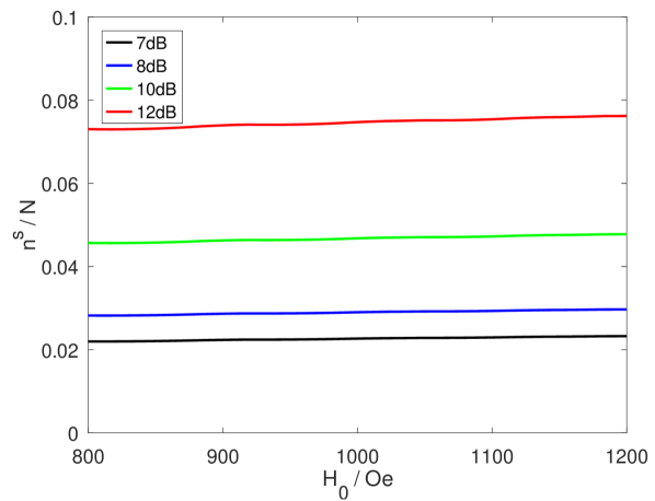
Figure 2: Dependence of the magnon density $n^{s}/N=\sum_{\bm{k}}n^{s}_{\bm{k}}/N$ on the external magnetic field strength $H_{0}$ in the stationary non-equilibrium state within S-theory given by Eq. (24a) for different pumping strengths. The maximum of $V_{\bm{k}}$ was chosen to be larger than the relaxation rate $\gamma_{\bm{k}}=2.19\times 10^{-3}$GHz. To describe the experiment of Noack et al Noack19 we have performed our calculations for a thin YIG film with thickness $d=22.8\,\mu$m (corresponding to $N=18422$) subject to a microwave field with frequency $\omega_{0}=13.857$ GHz.

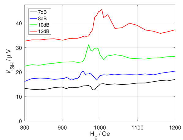
Figure 3: Experimental results for the inverse spin-Hall voltage $V_{\rm{ISH}}$ reproduced from Fig. 4 a) of Ref. [Noack19, ].

For comparision, we reproduce in Fig. 3 the experimental results for the inverse spin-Hall effect voltage from Fig. 4 a) of Ref. [Noack19, ], which is expected to be proportional to the density of pumped magnons. Obviously, in a certain range of magnetic fields the experimental data exhibit characteristic features which are missed by S-theory, which explains only the average linear growth of the observed magnon density with increasing magnetic field. An obvious reason for the failure of S-theory is that the phenomenological damping introduced by hand neither takes into account the kinematic constraints nor the microscopic magnon dynamics responsible for the dissipative effects which are essential for the emergence of a stationary non-equilibrium state in the pumped magnon gas. For a satisfactory explanation of the experimental data Noack19 reproduced in the lower part of Fig. 3 we should therefore use kinetic equations with microscopically derived collision integrals describing the relevant scattering processes. The collisionless kinetic equations (18) are then replaced by

$$\partial_{t}n_{\bm{k}}^{c}(t)+i\left[\tilde{V}_{\bm{k}}(t)\left(\tilde{p}_{{\bm{k}}}^{c}(t)\right)^{*}-\tilde{V}_{\bm{k}}^{*}(t)\tilde{p}_{{\bm{k}}}^{c}(t)\right] = I^{n}_{\bm{k}}(t),$$

$$\partial_{t}\tilde{p}_{{\bm{k}}}^{c}(t)+2i\tilde{E}_{\bm{k}}(t)\tilde{p}_{{\bm{k}}}^{c}(t)+i\tilde{V}_{\bm{k}}(t)\left[2n_{\bm{k}}^{c}(t)+1\right] = I^{p}_{\bm{k}}(t),$$

$$\partial_{t}\tilde{\psi}_{{\bm{k}}}(t)+i\tilde{E}_{\bm{k}}(t)\tilde{\psi}_{{\bm{k}}}(t)+i\tilde{V}_{\bm{k}}(t)\tilde{\psi}_{-{\bm{k}}}^{*}(t) = I^{\psi}_{\bm{k}}(t),$$

where all interactions beyond S-theory are taken into account via three types of collision integrals $I^{n}_{\bm{k}}(t)$, $I^{p}_{\bm{k}}(t)$, and $I^{\psi}_{\bm{k}}(t)$. These collision integrals should be derived from the Hamiltonian (2), including the cubic part $\mathcal{\tilde{H}}_{3}(t)$ which determines the damping to leading order in the small parameter $1/S$. In spite of many decades of theoretical research on pumped magnon gases,Suhl57 ; Schloemann60 ; Zakharov70 ; Zakharov74 ; Vinikovetskii79 ; Cherepanov93 ; Araujo74 ; Tsukernik75 ; Lavrinenko81 ; Zvyagin82 ; Zvyagin85 ; Lim88 ; Kalafati89 ; Lvov94 ; Zvyagin07 ; Rezende09 ; Kloss10 ; Safonov13 ; Slobodianiuk17 ; Hahn20 a complete derivation of the relevant collision integrals $I^{n}_{\bm{k}}(t)$, $I^{p}_{\bm{k}}(t)$, and $I^{\psi}_{\bm{k}}(t)$ and the subsequent numerical solution of the resulting kinetic equations cannot be found in the literature. In the rest of this work we will solve this technically very complicated problem using an unconventional approach to non-equilibrium many-body systems developed by J. Fricke Fricke97 which we review in Appendix B.

Before deriving in the following section explicit microscopic expressions for the collision integrals in Eq. (27) let us generalize the construction of a stationary solution with phenomenological damping discussed above by assuming that the collision integrals are of the form

$$I^{n}_{\bm{k}}(t) = \gamma^{n}_{\bm{k}}n_{\bm{k}}(t),$$ (28a)

$$I^{p}_{\bm{k}}(t) = \gamma^{p}_{\bm{k}}\tilde{p}_{\bm{k}}(t),$$ (28b)

where $\gamma^{n}_{\bm{k}}$ and $\gamma^{p}_{\bm{k}}$ are assumed to be constant in time and independent of the magnon distribution functions. For simplicity we assume that the expectation values of the magnon operators are negligible and set $I^{\psi}_{\bm{k}}(t)=0$. In this case the stationary non-equilibrium solution of Eq. (27) can easily be obtained analytically. The imaginary part of $\gamma^{p}_{\bm{k}}$ can be grouped together with the renormalized magnon energy $\tilde{E}_{\bm{k}}$ and we therefore modify the expression for the renormalized magnon energy as follows,

$$\tilde{E}_{\bm{k}}=E_{\bm{k}}-\frac{1}{2}\mathrm{Im}\gamma^{p}_{\bm{k}}+\frac{1}{N}\sum\limits_{\bm{q}}T_{{\bm{k}},{\bm{q}}}n_{\bm{q}}(t).$$ (29)

For $|V_{\bm{k}}|>\frac{1}{4}\gamma^{n}_{\bm{k}}\mathrm{Re}\gamma^{p}_{\bm{k}}$ the stationary non-equilibrium solution of Eq. (27) is then given by

$$n^{s}_{\bm{k}} = \sqrt{\frac{\mathrm{Re}\gamma^{p}_{\bm{k}}}{\gamma^{n}_{\bm{k}}}}\left|\tilde{p}_{\bm{k}}\right|,$$ (30a)

$$\tilde{p}^{s}_{\bm{k}} = -\left(\sqrt{1-\frac{\gamma^{n}_{\bm{k}}\mathrm{Re}\gamma^{p}_{\bm{k}}}{4V_{\bm{k}}^{2}}}+i\sqrt{\frac{\gamma^{n}_{\bm{k}}\mathrm{Re}\gamma^{p}_{\bm{k}}}{4V_{\bm{k}}^{2}}}\right)\left|\tilde{p}_{\bm{k}}\right|,$$

$$\left|\tilde{p}^{s}_{\bm{k}}\right| = N\frac{\sqrt{V_{\bm{k}}^{2}-\frac{1}{4}\gamma^{n}_{\bm{k}}\mathrm{Re}\gamma^{p}_{\bm{k}}}-|E_{\bm{k}}|\sqrt{\gamma^{n}_{\bm{k}}/\mathrm{Re}\gamma^{p}_{\bm{k}}}}{T_{{\bm{k}},{\bm{k}}}+\frac{1}{2}S_{{\bm{k}},{\bm{k}}}}.$$

Note that for $\frac{1}{2}\gamma^{n}_{\bm{k}}=\frac{1}{2}\gamma^{p}_{\bm{k}}\equiv\gamma_{\bm{k}}$ we recover the stationary solution within conventional S-theory Zakharov70 ; Zakharov74 given in Eqs. (24). Contrary to the case without collision integrals, the result for non-vanishing expectation values $\tilde{\psi}_{{\bm{k}}}$ differs as the collision integrals cannot be written in the form $\gamma^{n}_{\bm{k}}(n_{\bm{k}}+|\tilde{\psi}_{{\bm{k}}}|^{2})$.

IV Collision Integrals

In this section we present a microscopic derivation of the collision integrals $I^{n}_{\bm{k}}(t)$, $I^{p}_{\bm{k}}(t)$, and $I^{\psi}_{\bm{k}}(t)$ appearing in the kinetic equations (27). Given the fact that for YIG the effective spin $S\approx 14$ is rather large Kreisel09 , we work to leading order in $1/S$ where only the cubic part $\mathcal{\tilde{H}}_{3}(t)$ of the Hamiltonian in Eq. (12) has to be taken into account. The assumption that the experimentally observed fine structure of the inverse spin-Hall signal shown in Fig. 3 can be explained with the help of the scattering processes described by the cubic vertices contained in $\mathcal{\tilde{H}}_{3}(t)$ is also supported by the fact that the peaks and dips of the observed signal as a function of the magnetic field agree with the points where the splitting processes (in which one magnon is absorbed and two magnons are emitted) and the confluence processes (in which two magnons are absorbed and one magnon is emitted) described by the vertices in $\mathcal{\tilde{H}}_{3}(t)$ become kinematically possible Noack19 . Note that a finite cubic part $\mathcal{\tilde{H}}_{3}(t)$ of the magnon Hamiltonian arises entirely from dipole-dipole interactions. The corresponding scattering processes conserve energy and momentum, but do not conserve the number of magnons Filho00 . As we do not expect magnon-phonon interactions, magnon-defect interactions, and interactions with thermal optical magnons to be responsible for the effect observed in the experiment Noack19 we neglect these interactions.

In principle, the collision integrals can be derived using the Keldysh formalism Kamenev11 . However the Keldysh formalism has the disadvantage that it produces two-time correlations, whereas in our case we are only interested in equal-time correlations. Although the reduction of two-time correlations to equal-time correlations can be achieved by means of standard methods such as the generalized Kadanoff-Baym-Ansatz Lipavsky86 , in view of the complexity of the collision integrals for YIG we find it more efficient to use a method involving only equal-time correlations at every step of the calculation. We therefore use the method developed by J. Fricke Fricke97 , which allows us to to derive directly a hierarchy of coupled kinetic equations for equal-time correlations and provides us with a systematic scheme for decoupling the correlations for arbitrary order. To make this work self-contained, in Appendix B we outline the main features of this method.

IV.1 Collision integrals due to cubic interaction vertices

Consider first the diagonal collision integral $I^{n}_{\bm{k}}(t)$ appearing in the kinetic equation (LABEL:eq:dgl_n_ci) for the connected part $n^{c}_{\bm{k}}(t)$ of the diagonal magnon distribution. Using the method developed in Ref. [Fricke97, ] (which we review in Appendix B) and omitting for simplicity the time-arguments, we find

$$I^{n}_{\bm{k}}(t)=\frac{i}{\sqrt{N}} \sum\limits_{\bm{q}}\left[\frac{1}{2}\Gamma_{{\bm{k}};{\bm{q}},{{\bm{k}}-{\bm{q}}}}^{\bar{a}aa}e^{-i\omega_{0}t/2}\langle\tilde{a}_{\bm{q}}^{\dagger}\tilde{a}_{{\bm{k}}-{\bm{q}}}^{\dagger}\tilde{a}_{\bm{k}}\rangle^{c}-\mathrm{c.c.}\right.$$

$$\left.+(\Gamma_{{\bm{q}};{{\bm{q}}-{\bm{k}}},{\bm{k}}}^{\bar{a}aa})^{*}e^{i\omega_{0}t/2}\langle\tilde{a}_{\bm{q}}^{\dagger}\tilde{a}_{{\bm{q}}-{\bm{k}}}\tilde{a}_{\bm{k}}\rangle^{c}-\mathrm{c.c.}\right],$$

where we have used momentum conservation to carry out one of the summations. Here $\langle\tilde{a}_{\bm{q}}^{\dagger}\tilde{a}_{{\bm{k}}-{\bm{q}}}^{\dagger}\tilde{a}_{\bm{k}}\rangle^{c}$ and $\langle\tilde{a}_{\bm{q}}^{\dagger}\tilde{a}_{{\bm{q}}-{\bm{k}}}\tilde{a}_{\bm{k}}\rangle^{c}$ are connected equal-time correlations involving three magnon operators. In the graphical representation of Eq. (LABEL:eq:n_3pc) shown Fig. 4 these correlations are represented by empty circles with three external legs (correlation bubbles).

Figure 4: Diagrammatic representation of contributions to the collision integral $I^{n}_{\bm{k}}(t)$ given in (LABEL:eq:n_3pc) which determine the time-evolution of the connected diagonal distribution function $n^{c}_{\bm{k}}(t)$. For simplicity we do not draw the two conjugated diagrams obtained by flipping the direction of each arrow corresponding to the complex conjugated terms in Eq. (LABEL:eq:n_3pc). The symbols have the following meaning: Outgoing arrows represent creation operators, incoming arrows represent annihilation operators, and the black dots represent external or interaction vertices. The left diagram contains two external vertices and the interaction vertex $\Gamma_{{\bm{k}};{\bm{q}},{{\bm{k}}-{\bm{q}}}}^{\bar{a}aa}$; the empty circle (correlation bubble) represents the correlation $\langle\tilde{a}_{\bm{q}}^{\dagger}\tilde{a}_{{\bm{k}}-{\bm{q}}}^{\dagger}\tilde{a}_{\bm{k}}\rangle^{c}$. As the lines between the correlation bubble and the interaction vertex in the left diagram form a pair of equivalent lines we have to insert a prefactor of $1/2$ in front of the first vertex in Eq. (LABEL:eq:n_3pc). The right diagram contains the vertex $\Gamma^{\bar{a}\bar{a}a}_{{\bm{k}},{{\bm{q}}-{\bm{k}}};{\bm{q}}}$ and the correlation $\langle\tilde{a}_{\bm{q}}^{\dagger}\tilde{a}_{{\bm{q}}-{\bm{k}}}\tilde{a}_{\bm{k}}\rangle^{c}$.

Note that the diagrams shown in Fig. 4 differ from Feynman diagrams as they represent contributions to the differential equations for the correlations at a fixed time. Next, we express the three-point correlations in Eq. (LABEL:eq:n_3pc) in terms of the four-point correlations using the equation of motion. As a representative example, let us consider the correlation $\langle\tilde{a}^{\dagger}_{\bm{q}}\tilde{a}^{\dagger}_{{\bm{k}}-{\bm{q}}}\tilde{a}_{\bm{k}}\rangle^{c}$ in the first term on the right-hand side of Eq. (LABEL:eq:n_3pc) and explicitly evaluate only the diagram shown in Fig. 5. The other terms entering the equation of motion corresponding to the remaining diagrams have the same form and are represented by the dots in Eqs. (32)–34) below. The calculations leading to the collision integrals are analogous for all terms. The equation of motion implies

$$\left[\frac{d}{dt}+i\left(\epsilon_{\bm{k}}-\epsilon_{\bm{q}}-\epsilon_{{\bm{k}}-{\bm{q}}}\right)\right]\langle\tilde{a}^{\dagger}_{\bm{q}}\tilde{a}^{\dagger}_{{\bm{k}}-{\bm{q}}}\tilde{a}_{\bm{k}}\rangle^{c}=-\frac{i}{\sqrt{N}}\sum\limits_{{\bm{q}}^{\prime}}\left[\frac{1}{2}\left(\Gamma_{{\bm{k}};{\bm{q}}^{\prime},{\bm{k}}-{\bm{q}}^{\prime}}^{\bar{a}aa}\right)^{*}e^{i\omega_{0}t/2}\langle\tilde{a}^{\dagger}_{\bm{q}}\tilde{a}^{\dagger}_{{\bm{k}}-{\bm{q}}}\tilde{a}_{{\bm{q}}^{\prime}}\tilde{a}_{{\bm{k}}-{\bm{q}}^{\prime}}\rangle^{c}+...\right].$$ (32)

Integrating Eq. (32) over the time we obtain

$$\langle\tilde{a}^{\dagger}_{\bm{q}}\tilde{a}^{\dagger}_{{\bm{k}}-{\bm{q}}}\tilde{a}_{\bm{k}}\rangle^{c}=-\frac{i}{\sqrt{N}}\sum\limits_{{\bm{q}}^{\prime}}\left[\frac{1}{2}\int\limits_{t_{0}}^{t}dt^{\prime}\mathrm{e}^{-i\left(\epsilon_{\bm{k}}-\epsilon_{\bm{q}}-\epsilon_{{\bm{k}}-{\bm{q}}}\right)\left(t-t^{\prime}\right)}\left(\Gamma_{{\bm{k}};{\bm{q}}^{\prime},{\bm{k}}-{\bm{q}}^{\prime}}^{\bar{a}aa}\right)^{*}e^{i\omega_{0}t/2}\langle\tilde{a}^{\dagger}_{\bm{q}}\tilde{a}^{\dagger}_{{\bm{k}}-{\bm{q}}}\tilde{a}_{{\bm{q}}^{\prime}}\tilde{a}_{{\bm{k}}-{\bm{q}}^{\prime}}\rangle^{c}+...\right].$$ (33)

Finally, substituting Eq. (33) into Eq. (LABEL:eq:n_3pc) we obtain

$$I^{n}_{\bm{k}}(t) = \frac{1}{N}\sum\limits_{{\bm{q}},{\bm{q}}^{\prime}}\left[\frac{1}{2}\int\limits_{t_{0}}^{t}dt^{\prime}\cos\left[\left(\epsilon_{\bm{k}}-\epsilon_{\bm{q}}-\epsilon_{{\bm{k}}-{\bm{q}}}\right)\left(t-t^{\prime}\right)\right]\Gamma_{{\bm{k}};{\bm{q}},{{\bm{k}}-{\bm{q}}}}^{\bar{a}aa}\left(\Gamma_{{\bm{k}};{\bm{q}}^{\prime},{\bm{k}}-{\bm{q}}^{\prime}}^{\bar{a}aa}\right)^{*}\langle\tilde{a}^{\dagger}_{\bm{q}}\tilde{a}^{\dagger}_{{\bm{k}}-{\bm{q}}}\tilde{a}_{{\bm{q}}^{\prime}}\tilde{a}_{{\bm{k}}-{\bm{q}}^{\prime}}\rangle^{c}+...\right]$$

$$\underrightarrow{t_{0}\rightarrow-\infty} \frac{2\pi}{N}\sum\limits_{{\bm{q}},{\bm{q}}^{\prime}}\left[\frac{1}{2}\delta\left(\epsilon_{\bm{k}}-\epsilon_{\bm{q}}-\epsilon_{{\bm{k}}-{\bm{q}}}\right)\Gamma_{{\bm{k}};{\bm{q}},{{\bm{k}}-{\bm{q}}}}^{\bar{a}aa}\left(\Gamma_{{\bm{k}};{\bm{q}}^{\prime},{\bm{k}}-{\bm{q}}^{\prime}}^{\bar{a}aa}\right)^{*}\langle\tilde{a}^{\dagger}_{\bm{q}}\tilde{a}^{\dagger}_{{\bm{k}}-{\bm{q}}}\tilde{a}_{{\bm{q}}^{\prime}}\tilde{a}_{{\bm{k}}-{\bm{q}}^{\prime}}\rangle^{c}+...\right],$$ (34)

where in the last step we have taken the limit $t_{0}\rightarrow-\infty$ and the dots denote the contributions of the other diagrams. The other terms entering this equation represented by the dots are of the same form. Note that the terms with two annihilation operators or two creation operators within the two-particle correlations are complex. Therefore, there appears an exponential function with imaginary valued argument instead of the cosine function leading in the thermodynamic limit to a term of the same form as in Eq. (34) without the factor of two. In this way all terms entering the equation of motion for the one-particle distribution functions can be obtained from the diagrams. A complete list of all diagrams contributing to the equation of motion of the three-point correlations $\langle\tilde{a}^{\dagger}_{\bm{q}}\tilde{a}^{\dagger}_{{\bm{k}}-{\bm{q}}}\tilde{a}_{\bm{k}}\rangle^{c}$ and $\langle\tilde{a}_{\bm{q}}^{\dagger}\tilde{a}_{{\bm{q}}-{\bm{k}}}\tilde{a}_{\bm{k}}\rangle^{c}$ is shown in Fig. 18 of Appendix C.

Figure 5: One of the diagrams contributing to the equation of motion of the three-point correlation $\langle\tilde{a}^{\dagger}_{\bm{q}}\tilde{a}^{\dagger}_{{\bm{k}}-{\bm{q}}}\tilde{a}_{\bm{k}}\rangle^{c}$. This diagram, which corresponds to the term explicitly written out in Eq. (32), contains the interaction vertex $\Gamma^{\bar{a}\bar{a}a}_{{\bm{q}}^{\prime},{\bm{k}}-{\bm{q}}^{\prime};{\bm{k}}}$ and the four-point correlation $\langle\tilde{a}^{\dagger}_{\bm{q}}\tilde{a}^{\dagger}_{{\bm{k}}-{\bm{q}}}\tilde{a}_{{\bm{q}}^{\prime}}\tilde{a}_{{\bm{k}}-{\bm{q}}^{\prime}}\rangle^{c}$. As the lines between the correlation bubble and the interaction vertex are a pair of equivalent lines this diagram should be weighted by an extra factor of $1/2$.

The approach outlined above can also be used to obtain the off-diagonal collision integral $I^{p}_{\bm{k}}(t)$ in the kinetic equation (LABEL:eq:dgl_p_ci) for the off-diagonal distribution function $\tilde{p}_{{\bm{k}}}^{c}(t)$. In this case there are only two diagrams containing the relevant vertices shown in Fig. 6. The corresponding expression for the off-diagonal collision integral is

$$I^{p}_{\bm{k}}(t)=-i\frac{1}{\sqrt{N}}\sum\limits_{\bm{q}} \left[\frac{1}{2}\left(\Gamma_{{\bm{k}};{\bm{q}},{{\bm{k}}-{\bm{q}}}}^{\bar{a}aa}\right)^{*}e^{i\omega_{0}t/2}\langle\tilde{a}_{-{\bm{q}}}\tilde{a}_{{\bm{q}}-{\bm{k}}}\tilde{a}_{-{\bm{k}}}\rangle^{c}\right.$$

$$\left.+\Gamma_{{{\bm{q}}-{\bm{k}}};{\bm{q}},{\bm{k}}}^{\bar{a}aa}e^{-i\omega_{0}t/2}\langle\tilde{a}^{\dagger}_{\bm{q}}\tilde{a}_{{\bm{q}}-{\bm{k}}}\tilde{a}_{-{\bm{k}}}\rangle^{c}\right].$$

The correlation $\langle\tilde{a}_{-{\bm{q}}}\tilde{a}_{{\bm{q}}-{\bm{k}}}\tilde{a}_{-{\bm{k}}}\rangle^{c}$ in the first term leads for large times to a delta function of the form $\delta\left(\epsilon_{\bm{k}}+\epsilon_{\bm{q}}+\epsilon_{{\bm{k}}-{\bm{q}}}\right)$. Keeping in mind that the magnon dispersion $\epsilon_{\bm{k}}$ is positive for all momenta, this term does not contribute to the off-diagonal collision integral $I^{p}_{\bm{k}}(t)$ for large times. The diagrams contributing to the correlation $\langle\tilde{a}^{\dagger}_{\bm{q}}\tilde{a}_{{\bm{q}}-{\bm{k}}}\tilde{a}_{-{\bm{k}}}\rangle^{c}$ have already been discussed in the context of the diagonal collision integral $I^{n}_{\bm{k}}(t)$, see Fig. 18 in Appendix C. Finally, the collision integral $I^{\psi}_{\bm{k}}(t)$ entering the kinetic equation (27) for the expectation values $\tilde{\psi}_{\bm{k}}$ of the magnon operators vanishes,

$$I^{\psi}_{\bm{k}}(t)=0,$$ (36)

because there is no diagram contributing to the time-evolution of $\tilde{\psi}_{\bm{k}}(t)$ that is quadratic in the three-point vertices.

Figure 6: The two diagrams contributing to the time-evolution of the off-diagonal distribution function $p_{\bm{k}}=\langle\tilde{a}_{-{\bm{k}}}\tilde{a}_{\bm{k}}\rangle$. The diagrams correspond to the two terms on the right-hand side of Eq. (LABEL:eq:p_3pc). The left diagram contains the interaction vertex $\Gamma^{\bar{a}\bar{a}a}_{{\bm{q}},{{\bm{k}}-{\bm{q}}};{\bm{k}}}$ and the correlation $\langle\tilde{a}_{-{\bm{q}}}\tilde{a}_{{\bm{q}}-{\bm{k}}}\tilde{a}_{-{\bm{k}}}\rangle^{c}$. The left diagram should be multiplied by a factor of $1/2$ because the lines between the correlation bubble and the vertex are equivalent. The right diagram contains the vertex $\Gamma_{{{\bm{q}}-{\bm{k}}};{\bm{q}},{\bm{k}}}^{\bar{a}aa}$ and the correlation $\langle\tilde{a}^{\dagger}_{\bm{q}}\tilde{a}_{{\bm{q}}-{\bm{k}}}\tilde{a}_{-{\bm{k}}}\rangle^{c}$.

IV.2 Decoupling of the equations of motion for the connected correlations

So far, we have expressed the contributions to the collision integrals involving the various types of three-point vertices in terms of connected four-point correlations. The next step is to decouple the hierarchy of equations of motion by replacing the connected four-point correlations by one-point and connected two-point correlations. Keeping in mind that the only non-vanishing distribution functions are $n^{c}_{\bm{k}}$, $\tilde{p}_{{\bm{k}}}^{c}$, and $\tilde{\psi}_{{\bm{k}}}$ we find

$$\langle\tilde{a}^{\dagger}_{\bm{k}}\tilde{a}_{\bm{k}}\tilde{a}^{\dagger}_{\bm{q}}\tilde{a}_{\bm{q}}\rangle^{c} = -1!\langle\tilde{a}^{\dagger}_{\bm{k}}\tilde{a}_{\bm{k}}\rangle\langle\tilde{a}^{\dagger}_{\bm{q}}\tilde{a}_{\bm{q}}\rangle+2!\langle\tilde{a}^{\dagger}_{\bm{k}}\tilde{a}_{\bm{k}}\rangle\langle\tilde{a}^{\dagger}_{\bm{q}}\rangle\langle\tilde{a}_{\bm{q}}\rangle$$ (37)

$$+2!\langle\tilde{a}^{\dagger}_{\bm{k}}\rangle\langle\tilde{a}_{\bm{k}}\rangle\langle\tilde{a}^{\dagger}_{\bm{q}}\tilde{a}_{\bm{q}}\rangle-3!\langle\tilde{a}^{\dagger}_{\bm{k}}\rangle\langle\tilde{a}_{\bm{k}}\rangle\langle\tilde{a}^{\dagger}_{\bm{q}}\rangle\langle\tilde{a}_{\bm{q}}\rangle$$

$$= -n^{c}_{\bm{k}}n^{c}_{\bm{q}}+n^{c}_{\bm{k}}\left|\psi_{\bm{q}}\right|^{2}+n^{c}_{\bm{q}}\left|\psi_{\bm{k}}\right|^{2}$$

$$-3\left|\psi_{\bm{k}}\right|^{2}\left|\psi_{\bm{q}}\right|^{2}.$$

Analogous expressions can be written down for the other four-point correlations, so that the collision integrals can be expressed in terms of the two types of two-point correlations $n^{c}_{\bm{k}}(t)$ and $\tilde{p}^{c}_{\bm{k}}(t)$ and the non-equilibrium expectation values $\psi_{\bm{k}}(t)$ of the magnon operators. It is convenient to decompose the collision integrals as

$$I^{p}_{\bm{k}}=I^{p}_{{\bm{k}},\mathrm{in}}-I^{p}_{{\bm{k}},\mathrm{out}},$$ (38a)

$$I^{p}_{\bm{k}}=I^{p}_{{\bm{k}},\mathrm{in}}-I^{p}_{{\bm{k}},\mathrm{out}},$$ (38b)

where $I_{{\bm{k}},\mathrm{in}}$ is the in-scattering or arrival term, and $I_{{\bm{k}},\mathrm{out}}$ is the out-scattering or departure term. The explicit expressions for the various contributions to the collision integrals are rather cumbersome and are given in Eqs. (C1) - (C4) of Appendix C. Within the rotating-wave approximation the fast oscillating terms containing factors of $\mathrm{e}^{\pm i\omega_{0}t}$ should be neglected to be consistent with a similar approximation in the renormalized magnon dispersion $\tilde{E}_{\bm{k}}$ and the pumping energy $\tilde{V}_{\bm{k}}$.

V Explanation of the magnetic field dependence of the inverse spin-Hall signal in YIG

Having derived explicit expressions for the collision integrals $I^{n}_{\bm{k}}(t)$ and $I^{p}_{\bm{k}}(t)$ we can now construct stationary solutions of the kinetic equations (27) and determine the non-equilibrium magnon distribution which is proportional to the inverse spin-Hall signal observed in the experiment.Noack19 As discussed in Sec. III.2, in order to understand the magnetic field dependence of the inverse spin-Hall signal we need a microscopic understanding of the momentum-dependent magnon damping. In this section we first calculate the magnon damping in thermal equilibrium which we need in the subsequent calculation of the collision integrals. We then present an approximate solution of the kinetic equations (27) with microscopic collision integrals derived in Sec. IV and obtain excellent agreement with the experiment Noack19 .

V.1 Magnon damping in thermal equilibrium

In thermal equilibrium with temperature $T$ the normal magnon distribution is given by the Bose-Einstein distribution

$$n_{\bm{k}}=\frac{1}{\mbox{e}^{\epsilon_{\bm{k}}/T}-1}.$$ (39)

The magnon damping in equilibrium can then be obtained from the imaginary part of the magnon self-energy obtained within the imaginary-time (Matsubara) formalism. Alternatively, the magnon damping $\gamma^{n}_{\bm{k}}$ in equilibrium can be obtained by writing the departure term of the collision integral as

$$I^{n}_{{\bm{k}},\mathrm{out}}=\gamma^{n}_{\bm{k}}n_{\bm{k}},$$ (40)

where for simplicity we consider only the normal (diagonal) part $I^{n}_{{\bm{k}},\mathrm{out}}$ of the collision integral. To simplify the explicit evaluation of the damping $\gamma^{n}_{\bm{k}}$ let us assume that the momentum $\bm{k}$ is sufficiently large so that we can neglect the effect of dipole-dipole interactions on the magnon dispersion. In this regime the long-wavelength magnon dispersion is determined by the exchange interaction,

$$\epsilon_{\bm{k}}=\sqrt{A_{\bm{k}}^{2}-\left|B_{\bm{k}}\right|^{2}}\approx\left|A_{\bm{k}}\right|=h_{0}+\rho{\bm{k}}^{2},$$ (41)

with exchange stiffness

$$\rho=JSa^{2}.$$ (42)

In the expressions for the magnon dispersion given in Appendix A [see Eqs. (A9c) and (A11)] we can then set $B_{\bm{k}}=0$ and $V_{\bm{k}}=0$. According to Ref. [Kreisel09, ], for the effective exchange energy in YIG is $J\approx 1.29$K, the effective spin is $S\approx 14.2$, and the lattice constant is $a\approx 12.376$ Å. The Bogoliubov transformation from Holstein-Primakoff bosons $b_{\bm{k}}$ to magnon operators $a_{\bm{k}}$ is then not necessary so that we may identify the corresponding vertices, $\Gamma_{{\bm{k}}_{1};{\bm{k}}_{2},{\bm{k}}_{3}}^{\bar{a}aa}=\Gamma_{{\bm{k}}_{1};{\bm{k}}_{2},{\bm{k}}_{3}}^{\bar{b}bb}$. Moreover, in the regime where the magnon dispersion is dominated by the exchange energy we may neglect the diagonal elements of the dipolar tensor $D_{\bm{k}}^{\alpha\beta}$ defined in Eq. (A19). In the geometry shown in Fig. 1 the only non-zero elements of the dipolar tensor are then $D^{yz}_{\bm{k}}=D^{zy}_{\bm{k}}$, see Eq. (A19d). This greatly simplifies all quantities appearing in the kinetic equations for the magnon distribution. To get a rough estimate for the order of magnitude of the damping, let us also neglect the contributions from the off-diagonal distribution $p_{\bm{k}}(t)$ and the expectation values $\psi_{\bm{k}}$ of the magnon operators to the collision integral $I^{n}_{{\bm{k}},\mathrm{out}}$ in Eq. (40). In this approximation we obtain

$$\gamma^{n}_{\bm{k}}=\gamma^{n}_{{\bm{k}},\mathrm{con}}+\gamma^{n}_{{\bm{k}},\mathrm{split}},$$ (43)

where the contribution from the confluent process is

$$\gamma^{n}_{{\bm{k}},{\rm con}} = \frac{\pi}{N}\sum_{\bm{q}}\delta({\epsilon}_{\bm{k}}-{\epsilon}_{\bm{k}-\bm{q}}-{\epsilon}_{\bm{q}})$$ (44)

$$\times|\Gamma^{\bar{a}aa}_{\bm{k};\bm{q},\bm{k}-\bm{q}}|^{2}[n_{\bm{q}}+n_{\bm{k}-\bm{q}}+1],$$

and the contribution from the splitting process is

$$\gamma^{n}_{{\bm{k}},{\rm split}} = \frac{2\pi}{N}\sum_{\bm{q}}\delta({\epsilon}_{\bm{k}}+{\epsilon}_{\bm{q}-\bm{k}}-{\epsilon}_{\bm{q}})$$ (45)

$$\times|\Gamma^{\bar{a}aa}_{\bm{q};\bm{k},\bm{q}-\bm{k}}|^{2}[n_{\bm{q}-\bm{k}}-n_{\bm{q}}].$$

Note that these expressions can also be obtained directly from the diagonal part of the imaginary frequency magnon self-energy $\Sigma(\bm{k},i\omega)$ via analytic continuation,

$$\gamma^{n}_{\bm{k}}=-{\rm Im}\Sigma(\bm{k},\epsilon_{\bm{k}}+i0^{+}).$$ (46)

The Feynman diagrams for the self-energy corrections associated with the confluence and the splitting processes are shown in Fig. 7.

(a)

(b)

Figure 7: Feynman diagrams representing the contributions to the magnon self-energy which generate (a) the confluent and (b) the splitting contributions to the magnon damping given in Eqs. (44) and (45). Here the arrows represent the magnon propagators and the dots represent the cubic interaction vertices.

For vanishing wavevector $\bm{k}=0$ the confluent contribution has been carefully evaluated by Chernyshev Chernyshev12 . Here we are only interested in the range of wavevectors $\bm{k}$ where the magnon dispersion is dominated by the exchange energy so that it can be approximated by $\epsilon_{\bm{k}}=h_{0}+\rho\bm{k}^{2}$. Keeping in mind that in our geometry the only non-vanishing matrix elements of the dipolar tensor are $D^{yz}_{\bm{k}}=D^{zy}_{\bm{k}}$ and using Eq. (A19d) we find that the relevant cubic interaction vertex in Eqs. (44) and (45) is given by

$$\Gamma_{{\bm{k}}_{1};{\bm{k}}_{2},{\bm{k}}_{3}}^{\bar{a}aa} = \Gamma^{\bar{b}bb}_{{\bm{k}}_{1},{\bm{k}}_{2},{\bm{k}}_{3}}=\sqrt{\frac{S}{2}}\left(D^{zy}_{{\bm{k}}_{2}}+D^{yz}_{{\bm{k}}_{3}}\right)$$ (47)

$$\approx -\frac{\Delta}{\sqrt{2S}}\left(\frac{k_{2y}k_{2z}}{k_{2}^{2}}+\frac{k_{3y}k_{3z}}{k_{3}^{2}}\right),$$

where the energy scale $\Delta$ associated with the dipolar interaction is defined in Eq. (6). Since the experimentNoack19 has been performed at room temperature which is large compared with the typical magnon energies, we may approximate the equilibrium magnon distribution in Eqs. (44) and (45) by a Rayleigh-Jeans distribution,

$$n_{\bm{q}} \approx T/\epsilon_{\bm{q}},\;\;\;\;\;\;n_{{\bm{k}}-{\bm{q}}}\approx T/\epsilon_{{\bm{k}}-{\bm{q}}}.$$ (48)

Shifting the integration variable $\bm{q}=\bm{q}^{\prime}+\bm{k}/2$ in Eq. (44), we obtain for the ratio of the confluent magnon damping to the magnon energy at high temperatures,

$$\frac{\gamma^{n}_{\bm{k},{\rm con}}}{\epsilon_{\bm{k}}}=\frac{T}{8J}\left(\frac{\Delta}{h_{0}S}\right)^{2}\Theta(|\bm{k}|-\kappa)F_{\rm con}({\bm{k}}/{\kappa}),$$ (49)

where the threshold momentum $\kappa$ is defined by

$$\kappa^{2}=2h_{0}/\rho,$$ (50)

and the dimensionless function $F_{\rm con}(\bm{p})$ is defined via the following integral

$$F_{\rm con}(\bm{p}) = \int_{0}^{2\pi}\frac{d\varphi}{2\pi}\frac{1}{\Bigl{[}1+\frac{1}{2}\left(\bm{p}+\hat{\bm{q}}_{\varphi}\sqrt{p^{2}-1}\right)^{2}\Bigr{]}\Bigl{[}1+\frac{1}{2}\left(\bm{p}-\hat{\bm{q}}_{\varphi}\sqrt{p^{2}-1}\right)^{2}\Bigr{]}}$$ (51)

$$\times \left[\frac{\left(p_{y}+\sqrt{p^{2}-1}\cos\varphi\right)\left(p_{z}+\sqrt{p^{2}-1}\sin\varphi\right)}{\left(\bm{p}+\hat{\bm{q}}_{\varphi}\sqrt{p^{2}-1}\right)^{2}}+\frac{\left(p_{y}-\sqrt{p^{2}-1}\cos\varphi\right)\left(p_{z}-\sqrt{p^{2}-1}\sin\varphi\right)}{\left(\bm{p}-\hat{\bm{q}}_{\varphi}\sqrt{p^{2}-1}\right)^{2}}\right]^{2},\hskip 19.91692pt$$

where $\hat{\bm{q}}_{\varphi}=\bm{e}_{y}\cos\varphi+\bm{e}_{z}\sin\varphi$. At the threshold momentum $\bm{k}=\kappa\hat{\bm{k}}$ this reduces to

$$F_{\rm con}(\hat{\bm{k}})=\frac{16}{9}\hat{k}_{y}^{2}\hat{k_{z}^{2}}.$$ (52)

A numerical evaluation of $F_{\rm con}(p_{y},p_{z}=0)$ is shown in Fig. 8.

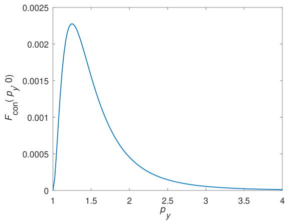
Figure 8: Numerical evaluation of the function $F_{\rm con}(p_{y},0)$ defined in Eq. (51) as a function of $p_{y}=k_{y}/\kappa$. For large $p_{y}$ we find that $F_{\rm con}(p_{y},0)\propto 1/p_{y}^{4}$.

A rough estimate for the order of magnitude of the confluent magnon damping for YIG at room temperature is given by the prefactor in Eq. (49), which yieldsNoack19

$$\frac{\gamma^{n}_{\bm{k},{\rm con}}}{\epsilon_{\bm{k}}} \approx \frac{T}{16J}\left(\frac{\Delta}{h_{0}S}\right)^{2}$$ (53)

$$= \frac{290K}{16\times 1.29K}\left(\frac{1750\;G}{1000\;G\times 14}\right)^{2}$$

$$= 14\times(0.125)^{2}\approx 0.22.$$

This indicates that at room temperature the damping due to magnon confluence can be substantial.

Next, consider the contribution from the splitting process to the magnon damping in equilibrium represented by the diagram (b) in Fig. 7. With the same approximations as above we obtain

$$\frac{\gamma^{n}_{\bm{k},{\rm split}}}{\epsilon_{\bm{k}}} = 2\pi Ta^{2}\int\frac{d^{2}q}{(2\pi)^{2}}\frac{\delta(h_{0}-2\rho\bm{k}\cdot\bm{q})}{\epsilon_{\bm{q}}\epsilon_{\bm{q}+\bm{k}}}$$ (54)

$$\times \frac{\Delta^{2}}{2S}\left[\hat{k}_{y}\hat{k}_{z}+\hat{q}_{y}\hat{q}_{z}\right]^{2}.$$

Setting for simplicity $k_{z}=0$, we see that the $\delta$-function enforces $q_{y}=q_{y}^{0}=h_{0}/(2\rho k_{y})$. The condition $|q_{y}^{0}|\leq\pi/a$ then reduces to $|k_{y}|>h_{0}a/(2\pi\rho)=\kappa^{2}a/(4\pi)$. With $\kappa a\ll 1$, it is clear that the splitting contribution to the magnon damping has a much lower threshold than the confluent contribution. Using the quadratic approximation (41) for the magnon dispersion and the definition (50) of $\kappa$ we find that for parametrically pumped magnons with $\epsilon_{\bm{k}}=\omega_{0}/2$ the condition $|{\bm{k}}|>\kappa$ is satisfied for

$$h_{0}<\frac{\omega_{0}}{6},$$ (55)

where the upper bound $\omega_{0}/6$ coincides with the magnetic field strength below which the confluent damping process is kinematically possible. On the other hand, for $h_{0}>\omega_{0}/6$ the damping is dominated by the splitting processes.

Unfortunately, the approximations made in this section are only valid for small pumping energy $\left|V_{\bm{k}}\right|$, whereas the experiment Noack19 has been performed in the regime of parametric instability where $\left|V_{\bm{k}}\right|>\left|E_{\bm{k}}\right|$. Therefore we expect that the estimates for the magnon damping in this subsection are not relevant for the experiment of Ref. [Noack19, ]. This is also confirmed by the linear magnetic field dependence of the damping due to the confluent and the splitting processes in thermal equilibrium shown in Fig. 9, which can be obtained by numerically evaluating Eqs. (44) and (45). In Fig. 10 we show the corresponding magnon density obtained by inserting this damping into the expression (24a) for the magnon distribution predicted by S-theory. Obviously, the magnetic-field dependence is linear in a wide range of fields and shows a small discontinuity at $H_{0}\approx 820$ Oe where the condition (55) is violated. By comparing Fig. 10 with the experimental result for the inverse spin-Hall voltage shown in Fig. 3, we conclude that by inserting the equilibrium magnon damping into the S-theory result for the stationary magnon density of the pumped magnon gas we cannot explain the experimental results.

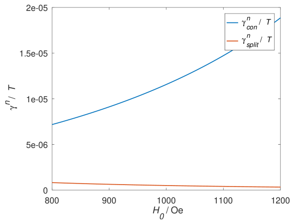
Figure 9: Magnetic field dependence of the magnon damping in thermal equilibrium due to the confluence and the splitting processes. The plotted damping rates $\gamma^{n}_{\mathrm{con}}$ and $\gamma^{n}_{\mathrm{split}}$ are obtained from Eqs. (49) and (54) by averaging over all momenta ${\bm{k}}$ satisfying $\epsilon_{\bm{k}}=\omega_{0}$. For the calculation we have assumed a film thickness of $d=22.8\,\mu$m and a pumping frequency $\omega_{0}=13.857$ GHz.

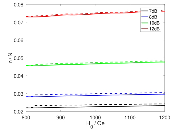
Figure 10: Magnetic field dependence of the stationry magnon density within S-theory given by Eq. (24a) for the same parameters as in Fig. 9. The continuous lines are obtained assuming a constant magnon damping $\gamma_{\bm{k}}=2.19\times 10^{-3}$GHz, while the dashed lines are obtained by substituting the equilibrium magnon damping shown in Fig. 9 into Eq. (24a).

V.2 Solution of the kinetic equations with microscopic collision integrals

In this section we show that the experimental results can be explained when the effect of collisions on the stationary distribution of the pumped magnon gas is taken into account microscopically within a non-equilibrium many-body approach where we approximately solve the kinetic equations (27) with collision integrals given in Appendix C. As it stands, this system of non-linear integro-differential equations is very complicated and we have not been able to solve it directly. Fortunately, we have found an approximation strategy which is sufficiently simple to allow for a numerical solution of the kinetic equations while it still contains the relevant physical processes which determine the detailed form of the experimentally observed inverse spin-Hall signal. Our strategy is to divide the magnons into the following two groups corresponding to different regimes in momentum space and different energy windows:

1. Parametric magnons are directly excited by the oscillating microwave field via parametric resonance. From S-theoryZakharov70 ; Zakharov74 ; Hahn20 we know that only magnons in a small area of the momentum space near the resonance surface defined by $\epsilon_{\bm{k}}=\omega_{0}/2$ are generated by the parametric pumping so that it is justified to assume that all parametric magnons fulfill the resonance condition $\epsilon_{\bm{k}}=\omega_{0}/2$.

2. Secondary magnons are created by confluence process of two parametric magnons. As a consequence, their energy $\epsilon_{\bm{k}}=\omega_{0}$ is twice as large as the energy of parametric magnons.

Assuming that the non-equilibrium magnon dynamics is dominated by these two groups of magnons, we can approximate the distribution of all other magnons in the collision integrals by the thermal equilibrium distribution. These approximations significantly simplify the collision integrals as the arguments of the delta functions only vanish if two of the energies correspond to parametric magnons and the other one to secondary magnons. The complexity of evaluating the collision integrals numerically is then greatly reduced. Neglecting the expectation values of the magnon operators we find from the general expressions for the collision integrals given in Appendix C that the collision integrals associated with the two different magnon groups can be written as

$$I^{n^{(1)}}_{\bm{k}} = \frac{2\pi}{N}\sum_{\stackrel{{\scriptstyle{\bm{q}}}}{{\stackrel{{\scriptstyle\epsilon_{\bm{q}}=\omega_{0}}}{{\epsilon_{{\bm{q}}-{\bm{k}}}=\omega_{0}/2}}}}}\biggl{[}\left|\Gamma_{{\bm{q}};{\bm{k}},{{\bm{q}}-{\bm{k}}}}^{\bar{a}aa}\right|^{2}\left(n^{(2)}_{\bm{q}}\left[1+n^{(1)}_{{\bm{q}}-{\bm{k}}}\right]-n^{(1)}_{\bm{k}}\left[n^{(1)}_{{\bm{q}}-{\bm{k}}}-n^{(2)}_{\bm{q}}\right]\right)$$ (56a)

$$\hskip 56.9055pt+\mathrm{Re}\left[\left(\Gamma_{{\bm{q}};{\bm{k}},{{\bm{q}}-{\bm{k}}}}^{\bar{a}aa}\right)^{*}\Gamma_{{{\bm{q}}-{\bm{k}}};{\bm{k}},{\bm{q}}}^{\bar{a}aa}(\tilde{p}^{(2)}_{{\bm{q}}})^{*}\tilde{p}^{(1)}_{{\bm{q}}-{\bm{k}}}\right]\biggr{]},$$

$$I^{n^{(2)}}_{\bm{k}} = \frac{2\pi}{N}\sum_{\stackrel{{\scriptstyle{\bm{q}}}}{{\stackrel{{\scriptstyle\epsilon_{\bm{q}}=\omega_{0}/2}}{{\epsilon_{{\bm{k}}-{\bm{q}}}=\omega_{0}/2}}}}}\biggl{[}\frac{1}{2}\left|\Gamma_{{\bm{k}};{\bm{q}},{{\bm{q}}-{\bm{k}}}}^{\bar{a}aa}\right|^{2}\left(n^{(1)}_{\bm{q}}n^{(1)}_{{\bm{k}}-{\bm{q}}}-n^{(2)}_{\bm{q}}\left[1+n^{(1)}_{\bm{q}}+n^{(1)}_{{\bm{k}}-{\bm{q}}}\right]\right)$$ (56b)

$$\hskip 56.9055pt-\mathrm{Re}\left[\Gamma_{{\bm{k}};{\bm{q}},{{\bm{k}}-{\bm{q}}}}^{\bar{a}aa}\left(\Gamma_{{\bm{q}};{{\bm{k}}-{\bm{q}}},{\bm{k}}}^{\bar{a}aa}\right)^{*}\tilde{p}^{(2)}_{\bm{k}}(\tilde{p}^{(1)}_{\bm{q}})^{*}+\left(\Gamma_{{\bm{k}};{\bm{q}},{{\bm{q}}-{\bm{k}}}}^{\bar{a}aa}\right)^{*}\Gamma_{{{\bm{k}}-{\bm{q}}};{\bm{k}},{\bm{q}}}^{\bar{a}aa}\tilde{p}^{(2)}_{\bm{k}}(\tilde{p}^{(1)}_{{\bm{k}}-{\bm{q}}})^{*}\right]\biggr{]},$$

$$I^{p^{(1)}}_{\bm{k}} = \frac{2\pi}{N}\sum_{\stackrel{{\scriptstyle{\bm{q}}}}{{\stackrel{{\scriptstyle\epsilon_{\bm{q}}=\omega_{0}}}{{\epsilon_{{\bm{q}}-{\bm{k}}}=\omega_{0}/2}}}}}\biggl{[}\Gamma_{{{\bm{q}}-{\bm{k}}};{\bm{k}},{\bm{q}}}^{\bar{a}aa}\left(\Gamma_{{\bm{k}};{{\bm{q}}-{\bm{k}}},{\bm{q}}}^{\bar{a}aa}\right)^{*}\tilde{p}^{(1)}_{{\bm{q}}-{\bm{k}}}\left(n^{(2)}_{\bm{q}}-n^{(1)}_{\bm{k}}\right)$$ (56c)

$$\hskip 51.21495pt-\left|\Gamma_{{{\bm{q}}-{\bm{k}}};{\bm{k}},{\bm{q}}}^{\bar{a}aa}\right|^{2}\tilde{p}^{(1)}_{\bm{k}}\left(1+n^{(1)}_{{\bm{q}}-{\bm{k}}}-\frac{1}{2}n^{(2)}_{\bm{q}}-\tilde{p}^{(2)}_{\bm{q}}\right)\biggr{]},$$

$$I^{p^{(2)}}_{\bm{k}} = 0,$$ (56d)

where $n^{(1)}_{\bm{k}}$ and $\tilde{p}^{(1)}_{\bm{k}}$ refer to the magnon distribution functions of parametric magnons and $n^{(2)}_{\bm{k}}$ and $\tilde{p}^{(2)}_{\bm{k}}$ refer to the secondary magnon group. When summing over the loop momentum ${\bm{q}}$, we have to implement the conditions $\epsilon_{\bm{k}}=\epsilon_{{\bm{q}}-{\bm{k}}}=\omega_{0}/2$, $\epsilon_{\bm{q}}=\omega_{0}$ in the collision integrals of the parametric magnon group, and the conditions $\epsilon_{\bm{k}}=\omega_{0}$ and $\epsilon_{\bm{q}}=\epsilon_{{\bm{k}}-{\bm{q}}}=\omega_{0}/2$ for the secondary magnon group. When all of these conditions can be fulfilled simultaneously, there is only one possible combination of wavevectors so that only a single term contributes to the sums in Eq. (56). In order to calculate the collision integrals numerically we thus have to find the specific combination of wavevectors that fulfill momentum and energy conservation. Then, we interpolate linearly between the magnon distribution functions defined on a finite grid in momentum space and evaluate the expressions (56). It is also possible that for certain parameters the conservation laws cannot be fulfilled, so that the collision integrals vanish in our approximation. All other magnons which do not belong to the above two groups are assumed to be in thermal equilibrium where the stationary distributions are given by the Bose-Einstein distribution (39) with $T=290$ K. We take the contribution of these equilibrium magnons to the damping of the non-equilibrium magnons into account using the equilibrium damping rates derived in Sec. V.1.

To obtain a self-consistent solution of the kinetic equations (27) with collision integrals given by Eq. (56) we use the following iterative procedure: Initially, we completely neglect the collision integrals and use the stationary distribution (30) of the kinetic equations with phenomenological damping $\gamma^{n}_{\bm{k}}=\gamma^{p}_{\bm{k}}=\gamma_{0}=2.87\times 10^{-3}$GHz to construct the initial seed for the iteration. We then substitute the resulting stationary distribution back into our microscopic expressions (56) for the collision integrals and calculate a new estimate for the collision integrals. Next, we use the result to re-calculate a refined estimate for the stationary solution of the kinetic equations (30). To obtain new values for non-equilibrium damping rates $\gamma^{n^{(1)}}_{\bm{k}}$ and $\gamma^{p^{(1)}}_{\bm{k}}$ we assume that the terms proportional to $n^{(1)}_{\bm{k}}$ and $\tilde{p}^{(1)}_{\bm{k}}$ dominate the collision integrals and estimate $\gamma^{n^{(1)}}_{\bm{k}}$ and $\gamma^{p^{(1)}}_{\bm{k}}$ by $I^{n^{(1)}}_{\bm{k}}/n^{(1)}_{\bm{k}}$ and $I^{p^{(1)}}_{\bm{k}}/\tilde{p}^{(1)}_{\bm{k}}$. The result is again substituted into the right-hand side of the collision integrals (56) and the procedure is iterated again. Gradually, we obtain corrections to the initial estimate of the magnon distribution in the stationary non-equilibrium state. To control the convergence of this algorithm we estimate the error by evaluating the derivatives $\partial_{t}n_{\bm{k}}$ and $\partial_{t}\tilde{p}_{\bm{k}}$ given by the equations of motion (27) and summing up the absolute values for every magnon mode. This expression should vanish if our estimates for the magnon distributions approach the exact stationary solutions. If this estimated error tends to zero during the iteration, our algorithm has produced a self-consistent stationary solution of the kinetic equations (27). Note that the vanishing of the off-diagonal collision integral $I^{p^{(2)}}_{\bm{k}}$ associated with the secondary magnons implies that the stationary solution of the kinetic equation (30a) has the property that $n^{(2)}_{\bm{k}}$ vanishes independently of the value of $\tilde{p}^{(2)}_{\bm{k}}$.

In Fig. 11 we show our numerical results for a YIG film with thickness $d=22.8\mu$m (corresponding to $N=18423$) in a microwave field with frequency $\omega_{0}=13.857$GHz for four different pumping strengths between 7dB and 12dB, where the parameter controlling the pumping strength is $\langle V_{{\bm{k}}_{1}}-\gamma_{0}\rangle_{{\bm{k}}_{1}}$ with the average taken over all momenta ${\bm{k}}_{1}$ of parametric magnons. The magnon density shown in Fig. 11 is approximated by taking the sum over all magnon modes used for the calculations,

$$n^{s}=\sum_{i=1}^{N_{\theta}}n^{s}_{i},$$ (57)

where the momentum dependence of the magnon distribution functions are parameterized by the angle $\theta_{i}=\theta_{\bm{k}_{i}}$ of the in-plane wavevectors defined in Eq. (8) and we use $N_{\theta}=40$ angles of equal size in the interval $[0,\pi/2]$. The wavevectors ${\bm{k}}_{1}$ and ${\bm{k}}_{2}$ of parametric and secondary magnons for a given angle $\theta_{i}$ are calculated by solving the equations $\epsilon_{{\bm{k}}_{1}}=\omega_{0}/2$ and $\epsilon_{{\bm{k}}_{2}}=\omega_{0}$ numerically for ${\bm{k}}_{1}$ and ${\bm{k}}_{2}$ with magnon dispersion given by Eq. (4).

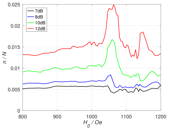
Figure 11: The magnon density obtained by the procedure described in Sec. V.2 for a thin YIG film of thickness $d=22.8\mu$m and $\omega_{0}=13.857$ GHz is plotted over the external field strength $H_{0}$ for four different pumping strengths. The parameter for the pumping strength is $\langle V_{{\bm{k}}_{1}}-\gamma_{0}\rangle_{{\bm{k}}_{1}}$ with the average taken over all momenta ${\bm{k}}_{1}$ of parametric magnons. Our theoretical result shown in this figure should be compared with the experimental results by Noack et al.Noack19 reproduced in Fig. 3.

Apart from a small offset in the overall field strength by about $50$ Oe, the main features of the experimentally observed line-shape of the inverse spin-Hall signal shown in Fig. 3 are reproduced remarkably well by our calculation. Recall that S-theory with phenomenological constant damping cannot explain this line-shape. In particular, the experimentally observed dip around $H_{0}\approx 1050$ Oe for small pumping strength which evolves into a peak at the same field for larger pumping strength is reproduced by our method. Note, however, that in the experiment these features appear at a slightly lower field of $H_{0}\approx 1000$ Oe. A possible explanation for this discrepancy in the overall field strength is the influence of cubic crystallographic and uni-axial anisotropy fields which can modify the saturation magnetization. It is therefore plausible that the experimentally relevant value of the saturation magnetization differs from the value of $1750$ G assumed in our calculation which can explain the $50$ Oe shift in the position of the peaks and dips in the upper and lower part of Fig. 11 .

To show that dip and the peak are related to the confluent magnon damping, we have plotted in Fig. 12 the cumulative damping rates $\gamma^{n}=\sum_{i=1}^{N_{\theta}}\gamma^{n}_{i}$ and ${\rm Re}\gamma^{p}=\sum_{i=1}^{N_{\theta}}{\rm Re}\gamma^{p}_{i}$ for the stationary non-equilibrium state we have obtained from our kinetic equations.

(a)

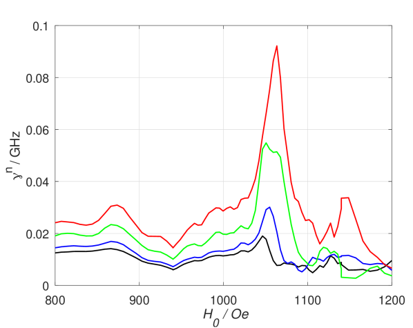
(b)

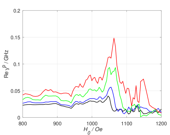
Figure 12: The damping defined by Eqs. (28) in the stationary non-equilibrium state shown in Fig. 11 is plotted over the external field strength $H_{0}$ for the same parameter values as in Fig. 11.

Obviously, the peaks in the cumulative magnon damping are observed at the same magnetic field strength where the enhancement of the magnon density takes place. Not all magnon modes show these enhancements. The distribution functions for most of the magnon modes still increase linearly with the external field strength and only a few magnon modes around $\theta_{\bm{k}}\approx 40^{\circ}$ have peaks between $H_{0}=1050$ Oe and $H_{0}=1100$ Oe.

It is interesting to compare the order of magnitude of the cumulative non-equilibrium damping $\gamma^{n}$ shown in the upper panel of Fig. 12 with the established value of the Gilbert damping used in phenomenological approaches for YIG Bender14 ; Hoffman13 ; Cornelissen16 . Usually the momentum-dependent damping $\gamma_{\bm{k}}$ is parameterized in terms of a dimensionless damping parameter $\alpha=\gamma_{{\bm{k}}}/(2\epsilon_{\bm{k}})$, where $\epsilon_{\bm{k}}$ is the magnon dispersion.Bender14 According to Refs. [Hoffman13, ; Cornelissen16, ] for thermal acoustic magnons in YIG the typical value of $\alpha$ is for small wavevectors of order $10^{-4}$. On the other hand, our cumulative non-equilibrium damping $\gamma^{n}$ in the upper panel of Fig. 12 is typically of order $0.02$ GHz, which yields a dimensionless damping parameter $\alpha\approx 1.4\times 10^{-3}$. We conclude that the non-equilibrium damping obtained within our microscopic approach is roughly an order of magnitude larger than the accepted phenomenological value of the equilibrium damping of thermal magnons in YIG.

The rather complicated dependence of the non-equilibrium magnon density on the external magnetic field shown in Fig. 12) cannot be reproduced within conventional S-theory where the microscopic collision integrals are replaced by a phenomenological relaxation rate. In the relevant parameter regime, S-theory predicts a linear dependence of the magnon density on the external field strength as shown in Fig. 2. Note also that within S-theory the damping is assumed to be strong so that only magnon modes near the maximum of the pumping energy $V_{\bm{k}}$ at $\theta_{\bm{k}}=90^{\circ}$ are significantly occupied. In fact, the magnon modes which we have identified to be responsible for the observed peaks and dips are assumed to be suppressed by the phenomenological damping in S-theory. Thus, it is evident that the experimentally observed structures in the non-equilibrium magnon density are caused by the confluence and splitting decay processes; the kinematic constraints controlling these processes are fully taken into account in our collision integrals which couple pairs of parametric magnons at special wavevectors depending on the external field strength. The mathematical structure of the equations of motion is complicated and leads to peak structures appearing in the collision integrals at certain field strengths. This in turn gives rise to similar structures in the field-dependent magnon density close to magnetic fields where confluent magnon decay is kinematically possible.

VI Summary and conclusions

In this work we have derived and solved kinetic equations for pumped magnons in YIG with collision integrals discribing dissipative effects associated with magnon decays. The collisionless limit of these equations has recently been discussed in Ref. [Hahn20, ]. However, to explain recent experimentel data Noack19 for the magnetic field dependence of the inverse spin-Hall voltage in the stationary non-equilibrium state of pumped magnons in YIG a microscopic understanding of magnon decays is crucial. We have derived the relevant collision integrals due to cubic interaction vertices using a systematic expansion in powers of connected equal-time correlations Fricke97 . We have obtained the collision integrals for the diagonal and off-diagonal distribution functions containing terms which are linear and quadratic in the magnon distribution functions as well as the expectation values of the magnon operators. In previous works these collision integrals were not taken into account due to their complexity or were only derived within Born approximation Vinikovetskii79 and evaluated in thermal equilibrium.

We have found a way to numerically solve the resulting kinetic equations within an approximation where only two groups of magnons are asumed to be driven out of equilibrium: parametric magnons that are generated by the pumping, and secondary magnons that are involved in confluence and splitting processes described by the microscopic collision integrals. We have explicitly constructed the stationary non-equilibrium solution of the kinetic equations for the pumped magnon gas.

Our results show in a large parameter regime a roughly linear magnetic field dependence of the magnon density, in agreement with previous results obtained within a collisionless kinetic theory. However, near the magnetic field strength where magnon decays (confluence and splitting processes) become kinematically allowed, we have obtained peak and dip structures in the magnon density, in good agreement with the experiment by Noack et al. Noack19 where the non-equilibrium magnon density has been measured via the inverse spin-Hall effect.

APPENDIX A: HAMILTONIAN FOR PUMPED MAGNONS IN YIG

Here we derive the magnon Hamiltonian for the parametrically pumped magnon gas in YIG following mainly Ref. [Kreisel09, ]. We start from the effective spin Hamiltonian for YIG Cherepanov93 ; Lvov94 ; Rezende09 ; Kloss10 ; Hick10 ; Rueckriegel14 ; Rezende06 ; Kreisel09 given in Eq. (1). The exchange couplings $J_{ij}$ assume the value $J\approx 1.29$ K for all pairs of nearest neighbor spins located at lattices sites $\bm{r}_{i}$ and $\bm{r}_{j}$, and the dipolar tensor is Kreisel09 ; Filho00

$$D_{ij}^{\alpha\beta}=\left(1-\delta_{ij}\right)\frac{\mu^{2}}{\left|\bm{r}_{ij}\right|^{3}}\left[3\hat{{r}}_{ij}^{\alpha}\hat{{r}}_{ij}^{\beta}-\delta^{\alpha\beta}\right],$$ (A1)

where $\mu$ is the magnetic moment of the spins, $\bm{r}_{ij}=\bm{r}_{i}-\bm{r}_{j}$, and $\hat{\bm{r}}_{ij}=\bm{r}_{ij}/\left|\bm{r}_{ij}\right|$. After Holstein-Primakoff transformation Holstein40 and expansion in powers of $1/S$ the spin Hamiltonian is mapped onto an effective boson Hamiltonian of the form (2) where the terms ${\cal{H}}_{i}$ can be expressed in terms of Holstein-Primakoff bosons $b_{i}$ and $b^{\dagger}_{i}$. The zeroth order contribution $\mathcal{H}_{0}(t)$ can be dropped as it does not contain any boson operators. Transforming to momentum space,

$$b_{i}=\frac{1}{\sqrt{N}}\sum\limits_{\bm{k}}\text{e}^{i{\bm{k}}\cdot\bm{r}_{i}}b_{\bm{k}},$$ (A2)

where $N$ is the total number of lattice sites, the contributions to the Hamiltonian up to fourth order in the bosons can be written as Hick10

$$\mathcal{H}_{2}(t) = \sum\limits_{\bm{k}}\left[A_{\bm{k}}b^{\dagger}_{\bm{k}}b_{\bm{k}}+\frac{B_{\bm{k}}}{2}\left(b^{\dagger}_{\bm{k}}b^{\dagger}_{-{\bm{k}}}+b_{-{\bm{k}}}b_{\bm{k}}\right)\right]$$ (A3a)

$$\hskip 22.76219pt+h_{1}\cos\left(\omega_{0}t\right)\sum\limits_{\bm{k}}b^{\dagger}_{\bm{k}}b_{\bm{k}},$$

$$\mathcal{H}_{3} = \frac{1}{\sqrt{N}}\sum\limits_{{\bm{k}}_{1},{\bm{k}}_{2},{\bm{k}}_{3}}\delta_{{\bm{k}}_{1}+{\bm{k}}_{2}+{\bm{k}}_{3},0}\frac{1}{2!}\left[\Gamma^{\bar{b}bb}_{1;2,3}b^{\dagger}_{-1}b_{2}b_{3}\right.$$ (A3b)

$$\hskip 45.5244pt\left.+\Gamma^{\bar{b}\bar{b}b}_{1,2;3}b^{\dagger}_{-1}b^{\dagger}_{-2}b_{3}\right],$$

$$\mathcal{H}_{4} = \frac{1}{N}\sum\limits_{{\bm{k}}_{1},\dots,{\bm{k}}_{4}}\delta_{{\bm{k}}_{1}+\dots+{\bm{k}}_{4},0}\left[\frac{1}{\left(2!\right)^{2}}\Gamma^{\bar{b}\bar{b}bb}_{1,2;3,4}b^{\dagger}_{-1}b^{\dagger}_{-2}b_{3}b_{4}\right.$$

$$\left.+\frac{1}{3!}\Gamma^{\bar{b}bbb}_{1;2,3,4}b^{\dagger}_{-1}b_{2}b_{3}b_{4}+\frac{1}{3!}\Gamma^{\bar{b}\bar{b}\bar{b}b}_{1,2,3;4}b^{\dagger}_{-1}b^{\dagger}_{-2}b^{\dagger}_{-3}b_{4}\right].$$

The vertices in (A3a)-(LABEL:eq:H4_ft) can be expressed in terms of the Fourier transforms of the exchange and dipolar couplings,

$$J_{\bm{k}} = \sum\limits_{i}\text{e}^{-i{\bm{k}}\cdot\bm{r}_{ij}}J_{ij},$$ (A4a)

$$D^{\alpha\beta}_{\bm{k}} = \sum\limits_{i}\text{e}^{-i{\bm{k}}\cdot\bm{r}_{ij}}D^{\alpha\beta}_{ij}.$$ (A4b)

The coefficients $A_{\bm{k}}$ and $B_{\bm{k}}$ in Eq.(A3a) are

$$A_{\bm{k}} = h_{0}+S\left(J_{\bm{0}}-J_{\bm{k}}\right)+S\left[D^{zz}_{\bm{0}}-\frac{1}{2}\left(D^{xx}_{\bm{k}}+D^{yy}_{\bm{k}}\right)\right],$$

$$B_{\bm{k}} = -\frac{S}{2}\left[D^{xx}_{\bm{k}}-2iD^{xy}_{\bm{k}}-D^{yy}_{\bm{k}}\right],$$ (A5b)

while the cubic vertices depend only on the dipolar tensor as follows,

$$\Gamma^{\bar{b}bb}_{1;2,3} = \sqrt{\frac{S}{2}}\left[D^{zy}_{{\bm{k}}_{2}}-iD^{zx}_{{\bm{k}}_{2}}+D^{zy}_{{\bm{k}}_{3}}-iD^{zx}_{{\bm{k}}_{3}}\right.$$ (A6a)

$$\left.+\frac{1}{2}\left(D^{zy}_{\mathbf{0}}-iD^{zx}_{\mathbf{0}}\right)\right],$$

$$\Gamma^{\bar{b}\bar{b}b}_{1,2;3} = \left(\Gamma^{\bar{b}bb}_{3;2,1}\right)^{*},$$ (A6b)

and the quartic vertices are

$$\Gamma^{\bar{b}\bar{b}bb}_{1,2;3,4} = -\frac{1}{2}\left[J_{{\bm{k}}_{1}+{\bm{k}}_{3}}+J_{{\bm{k}}_{2}+{\bm{k}}_{3}}+J_{{\bm{k}}_{1}+{\bm{k}}_{4}}+J_{{\bm{k}}_{2}+{\bm{k}}_{4}}\right.$$ (A7a)

$$\left.+D^{zz}_{{\bm{k}}_{1}+{\bm{k}}_{3}}+D^{zz}_{{\bm{k}}_{2}+{\bm{k}}_{3}}+D^{zz}_{{\bm{k}}_{1}+{\bm{k}}_{4}}+D^{zz}_{{\bm{k}}_{2}+{\bm{k}}_{4}}\right.$$

$$\left.-\sum\limits_{i=1}^{4}\left(J_{{\bm{k}}_{i}}-2D^{zz}_{{\bm{k}}_{i}}\right)\right],$$

$$\Gamma^{\bar{b}bbb}_{1;2,3,4} = \frac{1}{4}\left[D^{xx}_{{\bm{k}}_{2}}-2iD^{xy}_{{\bm{k}}_{2}}-D^{yy}_{{\bm{k}}_{2}}+D^{xx}_{{\bm{k}}_{3}}-2iD^{xy}_{{\bm{k}}_{3}}-D^{yy}_{{\bm{k}}_{3}}\right.$$ (A7b)

$$\left.+D^{xx}_{{\bm{k}}_{4}}-2iD^{xy}_{{\bm{k}}_{4}}-D^{yy}_{{\bm{k}}_{4}}\right],$$

$$\Gamma^{\bar{b}\bar{b}\bar{b}b}_{1,2,3;4} = \left(\Gamma^{\bar{b}bbb}_{4;1,2,3}\right)^{*}.$$ (A7c)

Next, we diagonalize the time-independent part of $\mathcal{H}_{2}(t)$ by introducing magnon annihilation and creation operators $a_{\bm{k}}$ and $a^{\dagger}_{\bm{k}}$ via the Bogoliubov transformation,

$$\left(\begin{array}[]{c}b_{\bm{k}}\\ b^{\dagger}_{-\bm{k}}\end{array}\right)=\left(\begin{array}[]{cc}u_{\bm{k}}&-v_{\bm{k}}\\ -v_{\bf{k}}^{\ast}&u_{\bm{k}}\end{array}\right)\left(\begin{array}[]{c}a_{\bm{k}}\\ a^{\dagger}_{-\bm{k}}\end{array}\right),$$ (A8)

where

$$u_{\bm{k}} = \sqrt{\frac{A_{\bm{k}}+\varepsilon_{\bm{k}}}{2\varepsilon_{\bm{k}}}},$$ (A9a)

$$v_{\bm{k}} = \frac{B_{\bm{k}}}{|B_{\bm{k}}|}\sqrt{\frac{A_{\bm{k}}-\varepsilon_{\bm{k}}}{2\varepsilon_{\bm{k}}}},$$ (A9b)

$$\varepsilon_{\bm{k}} = \sqrt{A_{\bm{k}}^{2}-|B_{\bm{k}}|^{2}}.$$ (A9c)

In terms of the magnon operators the time-dependent term in Eq. (A3a) leads to off-diagonal terms, so that the total quadratic Hamiltonian reads Hick10 ,

$$\mathcal{H}_{2}(t) = \sum\limits_{\bm{k}}\left[\varepsilon_{\bm{k}}a^{\dagger}_{\bm{k}}a_{\bm{k}}+\frac{\varepsilon_{\bm{k}}-A_{\bm{k}}}{2}\right.$$

$$\left.+h_{1}\cos\left(\omega_{0}t\right)\left(\frac{A_{\bm{k}}}{\varepsilon_{\bm{k}}}a^{\dagger}_{\bm{k}}a_{\bm{k}}-\frac{\varepsilon_{\bm{k}}-A_{\bm{k}}}{2\varepsilon_{\bm{k}}}\right)\right]$$

$$+\sum\limits_{\bm{k}}\left[V_{\bm{k}}\cos\left(\omega_{0}t\right)a^{\dagger}_{\bm{k}}a^{\dagger}_{-{\bm{k}}}+V_{\bm{k}}^{*}\cos\left(\omega_{0}t\right)a_{-{\bm{k}}}a_{\bm{k}}\right],$$

with pumping energy

$$V_{\bm{k}}=-\frac{h_{1}B_{\bm{k}}}{2\varepsilon_{\bm{k}}}.$$ (A11)

Expressing also the cubic and quartic parts of the Hamiltonian in terms of magnon operators we obtain Hick10

$$\mathcal{H}_{3} = \frac{1}{\sqrt{N}}\sum\limits_{{\bm{k}}_{1},{\bm{k}}_{2},{\bm{k}}_{3}}\delta_{{\bm{k}}_{1}+{\bm{k}}_{2}+{\bm{k}}_{3},0}\left[\frac{1}{2}\Gamma^{\bar{a}aa}_{1;2,3}a^{\dagger}_{-1}a_{2}a_{3}+\frac{1}{2}\Gamma^{\bar{a}\bar{a}a}_{1,2;3}a^{\dagger}_{-1}a^{\dagger}_{-2}a_{3}+\frac{1}{3!}\Gamma^{aaa}_{1,2,3}a_{1}a_{2}a_{3}+\frac{1}{3!}\Gamma^{\bar{a}\bar{a}\bar{a}}_{1,2,3}a^{\dagger}_{-1}a^{\dagger}_{-2}a^{\dagger}_{-3}\right],$$

$$\mathcal{H}_{4} = \frac{1}{N}\sum\limits_{{\bm{k}}_{1},{\bm{k}}_{2},{\bm{k}}_{3},{\bm{k}}_{4}}\delta_{{\bm{k}}_{1}+{\bm{k}}_{2}+{\bm{k}}_{3}+{\bm{k}}_{4},0}\left[\frac{1}{\left(2!\right)^{2}}\Gamma^{\bar{a}\bar{a}aa}_{1,2;3,4}a^{\dagger}_{-1}a^{\dagger}_{-2}a_{3}a_{4}+\frac{1}{3!}\Gamma^{\bar{a}aaa}_{1;2,3,4}a^{\dagger}_{-1}a_{2}a_{3}a_{4}\right.$$ (A13)

$$\left.+\frac{1}{3!}\Gamma^{\bar{a}\bar{a}\bar{a}a}_{1,2,3;4}a^{\dagger}_{-1}a^{\dagger}_{-2}a^{\dagger}_{-3}a_{4}+\frac{1}{4!}\Gamma^{aaaa}_{1,2,3,4}a_{1}a_{2}a_{3}a_{4}+\frac{1}{4!}\Gamma^{\bar{a}\bar{a}\bar{a}\bar{a}}_{1,2,3,4}a^{\dagger}_{-1}a^{\dagger}_{-2}a^{\dagger}_{-3}a^{\dagger}_{-4}\right],$$

with cubic vertices given by

$$\Gamma^{aaa}_{1,2,3} = -\Gamma^{\bar{b}bb}_{1;2,3}v_{1}u_{2}u_{3}-\Gamma^{\bar{b}bb}_{2;1,3}v_{2}u_{1}u_{3}-\Gamma^{\bar{b}bb}_{3;1,2}v_{3}u_{1}u_{3}+\Gamma^{\bar{b}\bar{b}b}_{1,2;3}v_{1}v_{2}u_{3}+\Gamma^{\bar{b}\bar{b}b}_{2,3;1}v_{2}v_{3}u_{1}+\Gamma^{\bar{b}\bar{b}b}_{1,3;2}v_{1}v_{3}u_{2},$$ (A14a)

$$\Gamma^{\bar{a}aa}_{1;2,3} = \Gamma^{\bar{b}bb}_{1;2,3}u_{1}u_{2}u_{3}+\Gamma^{\bar{b}bb}_{2;1,3}v_{1}v_{2}u_{3}+\Gamma^{\bar{b}bb}_{3;1,2}v_{1}v_{3}u_{2}-\Gamma^{\bar{b}\bar{b}b}_{3,2;1}v_{3}v_{2}v_{1}-\Gamma^{\bar{b}\bar{b}b}_{1,2;3}v_{2}u_{1}u_{3}-\Gamma^{\bar{b}\bar{b}b}_{1,3;2}v_{3}u_{1}u_{2},$$ (A14b)

$$\Gamma^{\bar{a}\bar{a}a}_{1,2;3} = \left(\Gamma^{\bar{a}aa}_{3;2,1}\right)^{*},$$ (A14c)

$$\Gamma^{\bar{a}\bar{a}\bar{a}}_{1,2,3} = \left(\Gamma^{aaa}_{1,2,3}\right)^{*},$$ (A14d)

and quartic vertices

$$\Gamma^{aaaa}_{1,2,3,4} = \Gamma^{\bar{b}\bar{b}bb}_{1,2;3,4}u_{1}u_{2}v_{3}v_{4}+\Gamma^{\bar{b}\bar{b}bb}_{1,3;2,4}u_{1}u_{3}v_{2}v_{4}+\Gamma^{\bar{b}\bar{b}bb}_{1,4;2,3}u_{1}u_{4}v_{2}v_{3}+\Gamma^{\bar{b}\bar{b}bb}_{2,3;1,4}u_{2}u_{3}v_{1}v_{4}$$ (A15a)

$$+\Gamma^{\bar{b}\bar{b}bb}_{2,4;1,3}u_{2}u_{4}v_{1}v_{3}+\Gamma^{\bar{b}\bar{b}bb}_{3,4;1,2}u_{3}u_{4}v_{1}v_{2}$$

$$-\Gamma^{\bar{b}bbb}_{4;1,2,3}u_{1}u_{2}u_{3}v_{4}-\Gamma^{\bar{b}bbb}_{3;1,2,4}u_{1}u_{2}u_{4}v_{3}-\Gamma^{\bar{b}bbb}_{2;1,3,4}u_{1}u_{3}u_{4}v_{2}-\Gamma^{\bar{b}bbb}_{1;2,3,4}u_{2}u_{3}u_{4}v_{1}$$

$$-\Gamma^{\bar{b}\bar{b}\bar{b}b}_{2,3,4;1}u_{1}v_{2}v_{3}v_{4}-\Gamma^{\bar{b}\bar{b}\bar{b}b}_{1,3,4;2}u_{2}v_{1}v_{3}v_{4}-\Gamma^{\bar{b}\bar{b}\bar{b}b}_{1,2,4;3}u_{3}v_{1}v_{2}v_{4}-\Gamma^{\bar{b}\bar{b}\bar{b}b}_{1,2,3;4}u_{4}v_{1}v_{2}v_{3},$$

$$\Gamma^{\bar{a}aaa}_{1;2,3,4} = -\Gamma^{\bar{b}\bar{b}bb}_{2,1;3,4}u_{2}v_{1}v_{3}v_{4}-\Gamma^{\bar{b}\bar{b}bb}_{3,1;2,4}u_{3}v_{1}v_{2}v_{4}-\Gamma^{\bar{b}\bar{b}bb}_{4,1;2,3}u_{4}v_{1}v_{2}v_{3}-\Gamma^{\bar{b}\bar{b}bb}_{2,3;1,4}u_{2}u_{3}u_{1}v_{4}$$ (A15b)

$$-\Gamma^{\bar{b}\bar{b}bb}_{2,4;1,3}u_{2}u_{4}u_{1}v_{3}-\Gamma^{\bar{b}\bar{b}bb}_{3,4;1,2}u_{3}u_{4}u_{1}v_{2}$$

$$+\Gamma^{\bar{b}bbb}_{1;2,3,4}u_{1}u_{2}u_{3}u_{4}+\Gamma^{\bar{b}bbb}_{4;3,2,1}u_{3}u_{2}v_{1}v_{4}+\Gamma^{\bar{b}bbb}_{3;4,2,1}u_{4}u_{2}v_{1}v_{3}+\Gamma^{\bar{b}bbb}_{2;4,3,1}u_{4}u_{3}v_{1}v_{2}$$

$$+\Gamma^{\bar{b}\bar{b}\bar{b}b}_{1,2,3;4}u_{4}u_{1}v_{2}v_{3}+\Gamma^{\bar{b}\bar{b}\bar{b}b}_{1,2,4;3}u_{3}u_{1}v_{2}v_{4}+\Gamma^{\bar{b}\bar{b}\bar{b}b}_{1,3,4;2}u_{2}u_{1}v_{3}v_{4}+\Gamma^{\bar{b}\bar{b}\bar{b}b}_{4,3,2;1}v_{4}v_{2}v_{3}v_{1},$$

$$\Gamma^{\bar{a}\bar{a}aa}_{1,2;3,4} = \Gamma^{\bar{b}\bar{b}bb}_{1,2;3,4}u_{1}u_{2}u_{3}u_{4}+\Gamma^{\bar{b}\bar{b}bb}_{1,3;4,2}u_{1}u_{4}v_{3}v_{2}+\Gamma^{\bar{b}\bar{b}bb}_{1,4;3,2}u_{1}u_{3}v_{4}v_{2}+\Gamma^{\bar{b}\bar{b}bb}_{2,3;4,1}u_{2}u_{4}v_{3}v_{1}$$ (A15c)

$$+\Gamma^{\bar{b}\bar{b}bb}_{2,4;3,1}u_{2}u_{3}v_{4}v_{1}+\Gamma^{\bar{b}\bar{b}bb}_{3,4;2,1}v_{1}v_{2}v_{3}v_{4}$$

$$-\Gamma^{\bar{b}bbb}_{4;3,2,1}u_{3}v_{2}v_{1}v_{4}-\Gamma^{\bar{b}bbb}_{3;4,2,1}u_{4}v_{2}v_{1}v_{3}-\Gamma^{\bar{b}bbb}_{2;3,4,1}u_{2}u_{3}u_{4}v_{1}-\Gamma^{\bar{b}bbb}_{1;3,4,2}u_{1}u_{3}u_{4}v_{2}$$

$$-\Gamma^{\bar{b}\bar{b}\bar{b}b}_{2,3,4;1}u_{2}v_{3}v_{4}v_{1}-\Gamma^{\bar{b}\bar{b}\bar{b}b}_{1,3,4;2}u_{1}v_{3}v_{4}v_{2}-\Gamma^{\bar{b}\bar{b}\bar{b}b}_{1,2,4;3}u_{1}u_{2}u_{3}v_{4}-\Gamma^{\bar{b}\bar{b}\bar{b}b}_{1,2,3;4}u_{1}u_{2}u_{4}v_{3},$$

$$\Gamma^{\bar{a}\bar{a}\bar{a}\bar{a}}_{1,2,3,4} = \Gamma^{aaaa}_{1,2,3,4},$$ (A15d)

$$\Gamma^{\bar{a}\bar{a}\bar{a}a}_{1,2,3;4} = \left(\Gamma^{\bar{a}aaa}_{4;3,2,1}\right)^{*}.$$ (A15e)

Finally, let us give simplified expressions for the Fourier transforms $J_{\bm{k}}$ and $D^{\alpha\beta}_{\bm{k}}$ for the geometry shown in Fig. 1 which reduce the complexity of the coefficients $A_{\bm{k}}$ and $B_{\bm{k}}$ and the higher-order vertices. For the energy scales probed in the experimentNoack19 it is sufficient to retain only the lowest magnon band, so that we can derive the dispersion from an effective in-plane Hamiltonian. The simplest approximation for the lowest transverse mode is the uniform mode approximation where we approximate the transverse modes by plane waves Kreisel09 . This approach is valid if the thickness $d$ of the YIG film is small compared to the extensions in $y$- and $z$-direction. Then we find

$$A_{\bm{k}} = h_{0}+JS\left[4-2\cos\left(k_{y}a\right)-2\cos\left(k_{z}a\right)\right]$$ (A16)

$$-\frac{S}{2}\left(D^{xx}_{\bm{k}}+D^{yy}_{\bm{k}}\right)+\frac{\Delta}{3},$$

$$B_{\bm{k}} = -\frac{S}{2}\left(D^{xx}_{\bm{k}}-D^{yy}_{\bm{k}}\right),$$ (A17)

where

$$\Delta=\frac{4\pi\mu^{2}S}{a^{3}}$$ (A18)

is the dipolar energy and the Fourier transformed elements of the dipolar tensor are Kreisel09

$$D^{xx}_{\bm{k}} = \frac{4\pi\mu^{2}}{a^{3}}\left[\frac{1}{3}-f_{\bm{k}}\right],$$ (A19a)

$$D^{yy}_{\bm{k}} = \frac{4\pi\mu^{2}}{a^{3}}\left[\frac{1}{3}-\left(1-f_{\bm{k}}\right)\sin^{2}\theta_{\bm{k}}\right],$$ (A19b)

$$D^{zz}_{\bm{k}} = \frac{4\pi\mu^{2}}{a^{3}}\left[\frac{1}{3}-\left(1-f_{\bm{k}}\right)\cos^{2}\theta_{\bm{k}}\right],$$ (A19c)

$$D^{yz}_{\bm{k}} = D^{zy}_{\bm{k}}=-\frac{2\pi\mu^{2}}{a^{3}}\sin\left(2\theta_{\bm{k}}\right),$$ (A19d)

$$D^{xy}_{\bm{k}} = D^{yx}_{\bm{k}}=0.$$ (A19e)

The form factor $f_{\bm{k}}$ is given in Eq. (7). For in-plane wavevectors $D^{yz}_{\bm{k}}=D^{zy}_{\bm{k}}$ is the only non-zero off-diagonal matrix element of the dipolar tensor. Within these approximations the expressions for the magnon energy $\epsilon_{\bm{k}}$ and the pumping energy $V_{\bm{k}}$ reduce to Eqs.(4) and (5) of the main text.

APPENDIX B: EXPANSION IN POWERS OF CONNECTED CORRELATIONS

In this appendix we review the method of deriving kinetic equations in terms of connected equal-time correlations developed by J. Fricke in Ref. [Fricke97, ]. In the following we refer to this method as the Fricke approach. In Sec. IV we have used this method to derive the leading contributions of the cubic interaction vertices to the collision integrals appearing in the kinetic equations (27). While it is also possible to use the Keldysh formalismKamenev11 for this task, the Fricke approach is more efficient for our purpose because it produces directly a hierarchy of coupled kinetic equations involving only equal-time correlations and provides us with a systematic decoupling scheme for correlations of arbitrary order. Note also that the Fricke approach generates an expansion of the collision integrals in powers of connected equal-time correlations and is therefore very convenient for including the effect of time-dependent non-Gaussian correlations in the non-equilibrium dynamics; in contrast, the Keldysh formalism relies on the perturbative expansion in terms of single-particle Green functions.

.1 Equations of motion

Consider the bosonic many-body system with second quantized Hamiltonian $H$ which may explicitly depend on time. In the Heisenberg picture the time-dependence of an operator $A(t)$ is given by the Heisenberg equation of motion,

$$i\frac{\mathrm{d}}{\mathrm{d}t}A(t)=\left[A(t),H\right].$$ (B1)

The expectation value of $A(t)$ is given by

$$\langle A\rangle_{t}=\mathrm{Tr}\left[\rho_{0}A(t)\right],$$ (B2)

where the density matrix $\rho_{0}$ specifies a mixture of states at the initial time $t_{0}$. The time-dependence of the expectation value is described by

$$i\frac{\mathrm{d}}{\mathrm{d}t}\langle A\rangle_{t}=\langle\left[A,H\right]\rangle_{t}.$$ (B3)

Writing $H=H_{0}^{t}+V$, where the one-particle part $H_{0}^{t}$ contains the terms that are quadratic in the bosonic operators and $V$ describes interactions, we obtain

$$i\frac{d}{dt}\langle A\rangle_{t}-\langle\left[A,H_{0}^{t}\right]\rangle_{t}=\langle\left[A,V\right]\rangle_{t}.$$ (B4)

The contribution of the one-particle Hamiltonian $H_{0}^{t}$ to the time-evolution of the system is easy to handle. In order to derive the contribution of the right hand side of Eq. (B4) containing the interaction Hamiltonian $V$, it is useful to introduce connected correlations.

.2 Connected correlations

In order to express expectation values of an arbitrary set of bosonic operators at the same time in terms of connected equal-time correlations we introduce the cluster expansion. Following again Ref. [Fricke97, ], let us consider a set of bosonic operators $B_{i}$ labeled by a set of integers $i\in\mathbb{N}$. The explicit expressions for the connected correlations contain sums over all partitions $P$ of an index set $I$ defined as the set of all non-empty disjoint subsets $J$ of $I$ with $\bigcup_{J\in P}J=I$. Furthermore, we define $B_{I}\equiv B_{i_{1}}\cdots B_{i_{k}}$ as the product of all operators with indices $i_{1},\dots,i_{k}$, where $i_{1}<\ldots<i_{k}$ and $I=\{i_{1},\dots,i_{k}\}$. In our case, the $B_{i}$ are bosonic field operators, i.e. linear combinations of bosonic creation operators $b_{j}^{\dagger}$ and annihilation operators $b_{j}$. They obey the commutation relations

$$\big{[}b_{i},b_{j}\big{]} = 0,\;\;\;\;\big{[}b_{i},b^{\dagger}_{j}\big{]}=\delta_{ij}.$$ (B5)

Since the operators do not commute in general, we keep track of their ordering by requireing that the indices $i_{k}$ within the sets $I$ are ordered as denoted above Fricke97 .

The connected correlations $\langle...\rangle^{c}$ can be defined recursively as follows, Baumann85

$$\langle B_{I}\rangle=\sum\limits_{P\in P_{I}}\prod\limits_{J\in P}\langle B_{J}\rangle^{c},$$ (B6)

where $P_{I}$ refers to the set of all partitions of $I$. With the help of Eq. (B6) we can write $n$-point correlation functions as sums over all partitions $P$ of the index set $I$ with each summand being the product of all correlations of the subsets $J\in P$. Note that the correlations preserve the ordering of the indices in the sets $J$. It is also possible to obtain an explicit expression for the connected correlations,Fricke97 ; Baumann85

$$\langle B_{I}\rangle^{c}=\sum\limits_{P\in P_{I}}\left(-1\right)^{\#P-1}\left(\#P-1\right)!\prod\limits_{J\in P}\langle B_{J}\rangle,$$ (B7)

where $\#I$ denotes to the cardinality of the set $I$ which we will refer to as the order of the correlations. For example, the connected correlations up to third order are, Fricke97

$$\langle B_{1}\rangle^{c} = \langle B_{1}\rangle,$$ (B8a)

$$\langle B_{1}B_{2}\rangle^{c} = \langle B_{1}B_{2}\rangle-\langle B_{1}\rangle\langle B_{2}\rangle,$$ (B8b)

$$\langle B_{1}B_{2}B_{3}\rangle^{c} = \langle B_{1}B_{2}B_{3}\rangle-\langle B_{1}B_{2}\rangle\langle B_{3}\rangle-\langle B_{1}\rangle\langle B_{2}B_{3}\rangle$$ (B8c)

$$-\langle B_{1}B_{3}\rangle\langle B_{2}\rangle+2\langle B_{1}\rangle\langle B_{2}\rangle\langle B_{3}\rangle.$$

The commutation relations (B5) imply that correlations with a permuted sequence of field operators differ. Using $\big{\langle}b_{1}b_{2}\big{\rangle}^{c}=\big{\langle}b_{1}b_{2}\big{\rangle}-\big{\langle}b_{1}\big{\rangle}\big{\langle}b_{2}\big{\rangle}$ it follows that the connected one-particle correlations are

$$\langle b_{i}b_{j}\rangle^{c}=\langle b_{j}b_{i}\rangle^{c},$$ (B9a)

$$\langle b_{i}b^{\dagger}_{j}\rangle^{c}=\delta_{ij}+\langle b^{\dagger}_{j}b_{i}\rangle^{c}.$$ (B9b)

On the other hand, in correlations of order greater than two the field operators permute trivially,Fricke97

$$\langle\cdots b_{i}b_{j}\cdots\rangle^{c} = \langle\cdots b_{j}b_{i}\cdots\rangle^{c},$$ (B10a)

$$\langle\cdots b_{i}b^{\dagger}_{j}\cdots\rangle^{c} = \langle\cdots b^{\dagger}_{j}b_{i}\cdots\rangle^{c}.$$ (B10b)

We note that only connected correlations of order $n=2$ obey a non-trivial commutation relation and are thus a special case. For this reason, we will refer to one-particle connected correlations as contractions. As we will see later, contractions play an important role for this method. A proof of Eqs. (B10a) and (B10b) can be found in Refs. [Baumann85, ; Fricke97, ].

The definition of the cluster expansion can also be extended to fermionic field operators in such a way that we obtain analogous equations. Then the correlations of order $n\neq 2$ anti-commuteFricke97 and hence sign rules have to be included. In this work we are only interested in bosonic operators.

.3 Linked-cluster theorem

We are interested in the time-evolution of $n$-point functions $\langle B_{I}\rangle_{t}=\langle B_{1}\cdots B_{k}\rangle_{t}$, where $B_{i}$ are linear combinations of bosonic field operators with $i\in I$. First, we simplify the interaction Hamiltonian $V$ in Eq. (B4) by assuming the form $V=B_{K}$. This can be justified by the fact that the equation of motion (B4) is a linear combination of the $B_{K}$. The linked-cluster theorem discussed in this appendix still holds for the full interaction Hamiltonian with the form of $V=\sum_{K}v_{K}B_{K}$.

The equation of motion of the expectation value $\langle B_{I}\rangle$ is given by Fricke97

$$i\frac{\mathrm{d}}{\mathrm{d}t}\langle B_{I}\rangle_{t}=\langle\left[B_{I},V\right]\rangle_{t}=\langle B_{I}B_{K}-B_{K}B_{I}\rangle_{t},$$ (B11)

where we have chosen $I$ and $K$ to be disjoint without loss of generality. As the connected correlation obey non-trivial commutation relations in general, we have to keep track of the sequence of indices of the operators inside the expectation values in Eq. (B11). Therefore we define $I+K$ as the set $I\cup K$ with the order relation given by the order relations of $I$ and $K$ respectively and the condition $i<k\ \forall i\in I,\ k\in K$. Note that the sets $I+K$ and $K+I$ are identical; their order relation differs though. For $J\in I+K$ we define $\tilde{J}$ as the identical set $J$ but with order relation of $K+I$, following Ref. [Fricke97, ].

It can be shown that there is a linked-cluster-theorem for the equation of motion of the connected correlations which is given by Fricke97

$$i\frac{\mathrm{d}}{\mathrm{d}t}\langle B_{I}\rangle^{c}_{t}=\sum\limits_{P\in P_{I,K}^{c}}\left(\prod\limits_{J\in P}\langle B_{J}\rangle^{c}_{t}-\prod\limits_{\tilde{J}\in P}\langle B_{\tilde{J}}\rangle^{c}_{t}\right),$$ (B12)

where $P_{I,K}^{c}$ is the set of all connected diagrams and is defined by

$$P_{I,K}^{c}\equiv\{P\in P_{I+K}|\forall J\in P:J\cap K\neq\emptyset\}.$$ (B13)

The right-hand side of Eq. (B12) can be further simplified. We have seen in the above section that only contractions which are one-particle connected correlations obey non-trivial commutation relations. Therefore the correlations $\langle B_{J}\rangle^{c}_{t}$ and $\langle B_{\tilde{J}}\rangle^{c}_{t}$ differ only for contraction and are identical for connected correlations of order $n\neq 2$. Obviously, the term within the brackets on the right-hand side of Eq. (B12) is non-zero only if it contains at least one contraction, so that in a diagrammatic representation (see below) only diagrams that contain contractions of external vertices with the interaction vertex contribute to the equation of motion of connected correlations.

.4 Diagrams

The diagrams introduced here differ from Feynman diagrams because they represent differential equations for the correlations. As a consequence, each diagrams contain only one interaction vertex. Moeover, each diagrams describe the time-evolution of a particular correlation at time $t$ so that there is no time or energy integration involved Fricke97 . Also, we introduce a new graphical symbol, the correlation bubble Schoeller94 representing the time-dependent correlations.

Let us now introduce the graphical elements of the diagrams. External vertices (Fig. 13) represent annihilation or creation operators. At least one external vertex is contracted with an interaction vertex (Fig. 14) which represents the interaction associated with a certain matrix element. Contractions (Fig. 15) are connected one-particle correlations. They are represented by their own graphical element as they play a special role for this method. Connected correlations of order $n\neq 2$ are represented by correlation bubbles (Fig. 16) Fricke97 . As there is not necessarily a conservation of particle numbers for bosons, the number of incoming lines can differ from the number of outgoing lines for interaction vertices and correlation bubbles.

Figure 13: External vertices represent annihilation operators with wavevector ${\bm{k}}^{\prime}_{1}$ or creation operators with wavevector ${\bm{k}}_{1}$.

Figure 14: Interaction vertices describe the interactions. They are connected with matrix elements $v_{i_{1},\dots,i_{r};j_{1},\dots,j_{s}}$.

Figure 15: The contraction $\big{\langle}b_{{\bm{k}}^{\prime}_{1}}^{\dagger}b_{{\bm{k}}_{1}}\rangle^{c}$. Contractions are connected correlations of order two. If the order is larger than two they are correlation bubbles (see Fig.16).

Figure 16: Correlation bubbles represent connected correlations, in this case $\langle b_{{\bm{k}}_{1}}\cdots b_{{\bm{k}}_{s}}b^{\dagger}_{{\bm{k}}^{\prime}_{r}}\cdots b^{\dagger}_{{\bm{k}}^{\prime}_{1}}\rangle^{c}_{t}$. Note that the order of the connected correlation has to be larger than two. Otherwise it is a contraction (see Fig.15).

Now we explain the rules for obtaining the time derivative of the $n$ point function $\langle b_{{\bm{k}}_{1}}\cdots b_{{\bm{k}}_{s}}b^{\dagger}_{{\bm{k}}^{\prime}_{r}}\cdots b^{\dagger}_{{\bm{k}}^{\prime}_{1}}\rangle_{t}$ due to interactions from the diagrams, where $n=r+s$. The cluster expansion of $\langle[b_{{\bm{k}}_{1}}\cdots b_{{\bm{k}}_{s}}b^{\dagger}_{{\bm{k}}^{\prime}_{r}}\cdots b^{\dagger}_{{\bm{k}}^{\prime}_{1}},V]\rangle_{t}$ leads to all possible diagrams where vertices are connected with contractions and correlation bubbles. The resulting diagrams contain $r+s$ external vertices and only one interaction vertex Fricke97 . The fact that there is only one interaction vertex simplifies the diagrammatic rules; there are no rules regarding time-ordering.

We start with the rule for the prefactor. From Eq. (B4) we get a factor of $(-i)$. Furthermore, we can write the interaction Hamiltonian in the form

$$V=\frac{1}{r!s!}\sum v_{i_{1},\dots,i_{r};i^{\prime}_{1},\dots,i^{\prime}_{s}}b^{\dagger}_{i_{1}}\cdots b^{\dagger}_{i_{s}}b_{i^{\prime}_{r}}\cdots b_{i^{\prime}_{1}}.$$ (B14)

Usually the interaction matrix elements $v_{i_{1},\dots,i_{r};i^{\prime}_{1},\dots,i^{\prime}_{s}}$ fulfill symmetry properties, causing the prefactor of $1/\left(r!s!\right)$ to drop out because permutating annihilation and creation operators in the interaction term gives the same contribution. However, there exists an exception: if two lines connected to a correlation bubble point into the same direction, permutating the operators yields the same graph and thus the prefactor remains Fricke97 .

The diagrammatic expansion of the equation of motion for the $n=r+s$-point function has the following structure,

$$\left[\frac{\mathrm{d}}{\mathrm{d}t}+i\left(\epsilon_{{\bm{k}}_{1}}+\dots+\epsilon_{{\bm{k}}_{s}}-\epsilon_{{\bm{k}}^{\prime}_{1}}-\dots-\epsilon_{{\bm{k}}^{\prime}_{r}}\right)\right]\langle b_{{\bm{k}}_{1}}\cdots b_{{\bm{k}}_{s}}b^{\dagger}_{{\bm{k}}^{\prime}_{r}}\cdots b^{\dagger}_{{\bm{k}}^{\prime}_{1}}\rangle_{t}=-i\sum_{\mathrm{diagrams}}\frac{1}{2^{n_{e}}}\sum\limits_{\begin{matrix}i_{1},\dots,i_{r}\\ j_{1},\dots,j_{s}\end{matrix}}v_{i_{1},\dots,i_{r},j_{1},\dots,j_{s}}X_{\mathrm{diagram}},$$ (B15)

where $X_{\mathrm{diagram}}$ is the collision term containing the contractions and correlations and $n_{e}$ denotes to the number of equivalent pairs of lines. By comparing Eq. (B15) with the general structure (B12) of the linked cluster expansion we notice that the collision term contains the difference of the partitions of $\langle b_{{\bm{k}}_{1}}\cdots b_{{\bm{k}}_{s}}b^{\dagger}_{{\bm{k}}^{\prime}_{r}}\cdots b^{\dagger}_{{\bm{k}}^{\prime}_{1}}V\rangle_{t}$ and the partitions of $\langle Vb_{{\bm{k}}_{1}}\cdots b_{{\bm{k}}_{s}}b^{\dagger}_{{\bm{k}}^{\prime}_{r}}\cdots b^{\dagger}_{{\bm{k}}^{\prime}_{1}}\rangle_{t}$. As connected correlations of order $n\neq 2$ obey trivial commutation relations, there will only be a difference of these two terms due to contractions. As a result, the collision term is a product of a several factors: First of all, $X_{\mathrm{diagram}}$ contains all correlations which are denoted by correlation bubbles. Furthermore, there are contributions from contractions. Contractions starting and ending at the interaction vertex give a normal-ordered contribution in the form $-\langle b^{\dagger}_{{\bm{k}}_{i}}b_{{\bm{k}}_{j}}\rangle^{c}_{t}$, contractions between external vertices give an anti-normal-ordered contribution of the form $\langle b_{{\bm{k}}_{i}}b^{\dagger}_{{\bm{k}}^{\prime}_{j}}\rangle^{c}_{t}$. Finally, there is a contribution from the remaining contractions connecting the external vertices with the interaction vertex. Labeling the diagram as shown in Fig. 17, this contribution has the form Fricke97

$$\left[\langle b_{{\bm{k}}_{1}}b^{\dagger}_{\bm{i}_{1}}\rangle^{c}_{t}\cdots\langle b_{{\bm{k}}_{s}}b^{\dagger}_{\bm{i}_{s}}\rangle^{c}_{t}\left(-\langle b^{\dagger}_{{\bm{k}}^{\prime}_{1}}b_{\bm{j}_{1}}\rangle^{c}_{t}\right)\cdots\left(-\langle b^{\dagger}_{{\bm{k}}^{\prime}_{r}}b_{\bm{j}_{r}}\rangle^{c}_{t}\right)\right.$$

$$\left.-\left(-\langle b^{\dagger}_{\bm{i}_{1}}b_{{\bm{k}}_{1}}\rangle^{c}_{t}\right)\cdots\left(-\langle b^{\dagger}_{\bm{i}_{s}}b_{{\bm{k}}_{s}}\rangle^{c}_{t}\right)\langle b_{\bm{j}_{1}}b^{\dagger}_{{\bm{k}}^{\prime}_{1}}\rangle^{c}_{t}\cdots\langle b_{\bm{j}_{r}}b^{\dagger}_{{\bm{k}}^{\prime}_{r}}\rangle^{c}_{t}\right].$$

Figure 17: Schematic diagram showing the interaction vertex. In total $r+s$ lines connect the interaction vertex with external vertices. The other lines go to correlation bubbles.

Diagrams without at least one contraction connecting an external vertex and an interaction vertex can be omitted, because the contributions of these diagrams vanish due to the fact that only contractions obey non-trivial commutation relations. Also, we only consider connected diagrams as unconnected diagrams do not contribute to the time-evolution of the correlations according to the linked-cluster theorem (B12).

APPENDIX C: COLLISION INTEGRALS FOR PUMPED MAGNONS IN YIG

Here we use the general formalism outlined in Appendix B to derive the collision integrals due to the cubic interaction vertices in the kinetic equations (27) describing the pumped magnon gas in YIG. The diagrams contributing to the correlations $\langle a^{\dagger}_{\bm{q}}a^{\dagger}_{{\bm{k}}-{\bm{q}}}a_{\bm{k}}\rangle^{c}$ and $\langle a^{\dagger}_{\bm{q}}a_{{\bm{q}}-{\bm{k}}}a_{\bm{k}}\rangle^{c}$ are shown in Fig. 18. Recall that these diagrams are different from Feynman diagrams as they describe the time-evolution of correlations. Therefore they only contain one interaction vertex and there is no time or energy integration associated with the diagrams. The diagrams shown in Fig. 18 represent contributions to the connected three-point correlations which determine the collision integrals as described in Sec. IV, see Eqs. (LABEL:eq:n_3pc) and (LABEL:eq:p_3pc). For the collision integrals associated with the diagonal distribution function we obtain for the arrival term

Figure 18: Diagrammatic representation of all terms contributing to the time-evolution of the correlation $\langle a^{\dagger}_{\bm{q}}a^{\dagger}_{{\bm{k}}-{\bm{q}}}a_{\bm{k}}\rangle^{c}$ (left set of diagrams) and to the correlation $\langle a^{\dagger}_{\bm{q}}a_{{\bm{q}}-{\bm{k}}}a_{\bm{k}}\rangle^{c}$ (right set of diagrams).

$$I_{{\bm{k}},\mathrm{in}}^{n} = \frac{2\pi}{N}\sum\limits_{\bm{q}}\Biggl{\{}\frac{1}{2}\delta\left(\varepsilon_{\bm{k}}-\varepsilon_{\bm{q}}-\varepsilon_{{\bm{k}}-{\bm{q}}}\right)\left|\Gamma_{{\bm{k}};{\bm{q}},{{\bm{k}}-{\bm{q}}}}^{\bar{a}aa}\right|^{2}n^{c}_{\bm{q}}n^{c}_{{\bm{k}}-{\bm{q}}}+\delta\left(\varepsilon_{\bm{k}}+\varepsilon_{{\bm{k}}-{\bm{q}}}-\varepsilon_{\bm{q}}\right)\left|\Gamma_{{\bm{q}};{\bm{k}},{{\bm{q}}-{\bm{k}}}}^{\bar{a}aa}\right|^{2}n^{c}_{\bm{q}}\left(1+n^{c}_{{\bm{q}}-{\bm{k}}}\right)$$ (C1)

$$\hskip 34.1433pt+\delta\left(\varepsilon_{\bm{k}}-\varepsilon_{\bm{q}}-\varepsilon_{{\bm{k}}-{\bm{q}}}\right)\Gamma_{{\bm{k}};{\bm{q}},{{\bm{k}}-{\bm{q}}}}^{\bar{a}aa}\sum\limits_{{\bm{q}}_{1}^{\prime},{\bm{q}}_{2}^{\prime}}\delta_{{\bm{q}}_{1}^{\prime}+{\bm{q}}_{2}^{\prime}-{\bm{k}},0}\biggr{[}\Gamma_{{\bm{q}}_{1}^{\prime};-{\bm{q}}_{2}^{\prime},{\bm{k}}}^{\bar{a}aa}e^{-i\omega_{0}t}\langle\tilde{a}_{\bm{q}}^{\dagger}\tilde{a}_{{\bm{q}}-{\bm{k}}}\tilde{a}_{-{\bm{q}}_{2}^{\prime}}^{\dagger}\tilde{a}_{{\bm{q}}_{1}^{\prime}}\rangle^{c}$$

$$\hskip 227.62204pt+\frac{1}{2}\left(\Gamma_{{\bm{k}};{\bm{q}}_{1}^{\prime},{\bm{q}}_{2}^{\prime}}^{\bar{a}aa}\right)^{*}\langle\tilde{a}_{\bm{q}}^{\dagger}\tilde{a}_{{\bm{q}}-{\bm{k}}}\tilde{a}_{{\bm{q}}_{1}^{\prime}}\tilde{a}_{{\bm{q}}_{2}^{\prime}}\rangle^{c}\biggr{]}$$

$$\hskip 34.1433pt+\delta\left(\epsilon_{\bm{k}}+\epsilon_{{\bm{q}}-{\bm{k}}}-\epsilon_{\bm{q}}\right)\left(\Gamma_{{\bm{q}};{\bm{k}},{{\bm{q}}-{\bm{k}}}}^{\bar{a}aa}\right)^{*}\sum\limits_{{\bm{q}}_{1}^{\prime},{\bm{q}}_{2}^{\prime}}\delta_{{\bm{q}}_{1}^{\prime}+{\bm{q}}_{2}^{\prime}-{\bm{k}},0}\biggl{[}\frac{1}{2}\left(\Gamma_{{\bm{k}};{\bm{q}}_{1}^{\prime},{\bm{q}}_{2}^{\prime}}^{\bar{a}aa}\right)^{*}e^{i\omega_{0}t}\langle\tilde{a}^{\dagger}_{\bm{q}}\tilde{a}^{\dagger}_{{{\bm{k}}-{\bm{q}}}}\tilde{a}_{{\bm{q}}_{1}^{\prime}}\tilde{a}_{{\bm{q}}_{2}^{\prime}}\rangle^{c}$$

$$\hskip 239.00314pt+\Gamma_{{\bm{q}}_{1}^{\prime};{\bm{k}},-{\bm{q}}_{2}^{\prime}}^{\bar{a}aa}\langle\tilde{a}_{\bm{q}}^{\dagger}\tilde{a}_{{\bm{k}}-{\bm{q}}}^{\dagger}\tilde{a}_{{\bm{q}}_{1}^{\prime}}\tilde{a}_{-{\bm{q}}_{2}^{\prime}}^{\dagger}\rangle^{c}\biggr{]}\Biggr{\}},$$

and for the departure term

$$I_{{\bm{k}},\mathrm{out}}^{n} = \frac{2\pi}{N}\sum\limits_{\bm{q}}\Biggl{\{}\frac{1}{2}\delta\left(\varepsilon_{\bm{k}}-\varepsilon_{\bm{q}}-\varepsilon_{{\bm{k}}-{\bm{q}}}\right)\left|\Gamma_{{\bm{k}};{\bm{q}},{{\bm{k}}-{\bm{q}}}}^{\bar{a}aa}\right|^{2}n^{c}_{\bm{k}}\left(1+n^{c}_{\bm{q}}+n^{c}_{{\bm{k}}-{\bm{q}}}\right)$$ (C2)

$$\hskip 34.1433pt+\delta\left(\varepsilon_{\bm{k}}+\varepsilon_{{\bm{q}}-{\bm{k}}}-\varepsilon_{\bm{q}}\right)\left|\Gamma_{{\bm{q}};{\bm{k}},{{\bm{q}}-{\bm{k}}}}^{\bar{a}aa}\right|^{2}n^{c}_{\bm{k}}\left(n^{c}_{{\bm{q}}-{\bm{k}}}-n^{c}_{\bm{q}}\right)$$

$$\hskip 34.1433pt+\delta\left(\varepsilon_{\bm{k}}-\varepsilon_{\bm{q}}-\varepsilon_{{\bm{k}}-{\bm{q}}}\right)\Gamma_{{\bm{k}};{\bm{q}},{{\bm{k}}-{\bm{q}}}}^{\bar{a}aa}\sum\limits_{{\bm{q}}_{1}^{\prime},{\bm{q}}_{2}^{\prime}}\delta_{{\bm{q}}_{1}^{\prime}+{\bm{q}}_{2}^{\prime}-{\bm{k}},0}\biggl{[}\frac{1}{2}\Gamma_{{\bm{q}};{\bm{q}}_{1}^{\prime},{\bm{q}}_{2}^{\prime}}^{\bar{a}aa}e^{i\omega_{0}t}\langle\tilde{a}_{\bm{k}}\tilde{a}_{{\bm{q}}-{\bm{k}}}\tilde{a}^{\dagger}_{{\bm{q}}_{1}^{\prime}}\tilde{a}^{\dagger}_{{\bm{q}}_{2}^{\prime}}\rangle^{c}$$

$$\hskip 79.66771pt+\left(\Gamma_{{\bm{q}}_{1}^{\prime};-{\bm{q}}_{2}^{\prime},{\bm{q}}}^{\bar{a}aa}\right)^{*}\langle\tilde{a}_{\bm{k}}\tilde{a}_{{\bm{q}}-{\bm{k}}}\tilde{a}_{{\bm{q}}_{1}^{\prime}}^{\dagger}\tilde{a}_{-{\bm{q}}_{2}^{\prime}}\rangle^{c}-\Gamma_{{\bm{q}}_{2}^{\prime};-{\bm{q}}_{1}^{\prime},{{\bm{q}}-{\bm{k}}}}^{\bar{a}aa}e^{i\omega_{0}t}\langle\tilde{a}_{\bm{k}}\tilde{a}_{\bm{q}}^{\dagger}\tilde{a}_{-{\bm{q}}_{1}^{\prime}}^{\dagger}\tilde{a}_{{\bm{q}}_{2}^{\prime}}\rangle^{c}$$

$$\hskip 227.62204pt-\frac{1}{2}\left(\Gamma_{{{\bm{q}}-{\bm{k}}};-{\bm{q}}_{1}^{\prime},{\bm{q}}_{2}^{\prime}}^{\bar{a}aa}\right)^{*}\langle\tilde{a}_{\bm{k}}\tilde{a}_{\bm{q}}^{\dagger}\tilde{a}_{-{\bm{q}}_{1}^{\prime}}\tilde{a}_{{\bm{q}}_{2}^{\prime}}\rangle^{c}\biggr{]}$$

$$\hskip 34.1433pt+\delta\left(\varepsilon_{\bm{k}}+\varepsilon_{{\bm{q}}-{\bm{k}}}-\varepsilon_{\bm{q}}\right)\left(\Gamma_{{\bm{q}};{\bm{k}},{{\bm{q}}-{\bm{k}}}}^{\bar{a}aa}\right)^{*}\sum\limits_{{\bm{q}}_{1}^{\prime},{\bm{q}}_{2}^{\prime}}\delta_{{\bm{q}}_{1}^{\prime}+{\bm{q}}_{2}^{\prime}-{\bm{k}},0}\biggl{[}\left(\Gamma_{{\bm{q}}_{1}^{\prime};{\bm{q}}_{2}^{\prime},{\bm{q}}}^{\bar{a}aa}\right)^{*}e^{i\omega_{0}t}\langle\tilde{a}_{\bm{k}}\tilde{a}_{{\bm{k}}-{\bm{q}}}^{\dagger}\tilde{a}_{{\bm{q}}_{1}^{\prime}}^{\dagger}\tilde{a}_{{\bm{q}}_{2}^{\prime}}\rangle^{c}$$

$$\hskip 108.12047pt+\frac{1}{2}\Gamma_{{\bm{q}};{\bm{q}}_{1}^{\prime},-{\bm{q}}_{2}^{\prime}}^{\bar{a}aa}\langle\tilde{a}_{\bm{k}}\tilde{a}_{{\bm{k}}-{\bm{q}}}^{\dagger}\tilde{a}_{{\bm{q}}_{1}^{\prime}}^{\dagger}\tilde{a}_{-{\bm{q}}_{2}^{\prime}}^{\dagger}\rangle^{c}+\frac{1}{2}\Gamma_{{{\bm{k}}-{\bm{q}}};{\bm{q}}_{1}^{\prime},-{\bm{q}}_{2}^{\prime}}^{\bar{a}aa}\langle\tilde{a}_{\bm{k}}\tilde{a}_{\bm{q}}^{\dagger}\tilde{a}_{{\bm{q}}_{1}^{\prime}}^{\dagger}\tilde{a}_{-{\bm{q}}_{2}^{\prime}}^{\dagger}\rangle^{c}$$

$$\hskip 81.09035pt+\frac{1}{2}\left(\Gamma_{{\bm{q}}_{2}^{\prime};{\bm{q}}_{1}^{\prime},{{\bm{k}}-{\bm{q}}}}^{\bar{a}aa}\right)^{*}e^{i\omega_{0}t}\langle\tilde{a}_{\bm{k}}\tilde{a}_{\bm{q}}^{\dagger}\tilde{a}_{{\bm{q}}_{1}^{\prime}}\tilde{a}_{{\bm{q}}_{2}^{\prime}}\rangle^{c}+\left(\Gamma_{{\bm{q}}_{1}^{\prime};{\bm{q}}_{2}^{\prime},{{\bm{k}}-{\bm{q}}}}^{\bar{a}aa}\right)^{*}e^{i\omega_{0}t}\langle\tilde{a}_{\bm{k}}\tilde{a}_{{\bm{q}}}^{\dagger}\tilde{a}_{{\bm{q}}_{1}^{\prime}}^{\dagger}\tilde{a}_{{\bm{q}}_{2}^{\prime}}\rangle^{c}\biggr{]}\Biggr{\}}.$$

For the collision integrals of the off-diagonal distribution function we obtain for the arrival term

$$I_{{\bm{k}},\mathrm{in}}^{p} = \frac{2\pi}{N}\sum\limits_{\bm{q}}\Biggl{\{}\delta\left(\varepsilon_{\bm{k}}+\varepsilon_{{\bm{q}}-{\bm{k}}}-\varepsilon_{\bm{q}}\right)\Gamma_{{{\bm{q}}-{\bm{k}}};{\bm{q}},-{\bm{k}}}^{\bar{a}aa}\Gamma_{{\bm{q}};{{\bm{q}}-{\bm{k}}},{\bm{k}}}^{\bar{a}aa}n^{c}_{\bm{q}}\left(1+n^{c}_{{\bm{q}}-{\bm{k}}}\right)$$ (C3)

$$\hskip 34.1433pt+\sum\limits_{{\bm{q}}_{1}^{\prime},{\bm{q}}_{2}^{\prime}}\delta\left(\varepsilon_{\bm{k}}+\varepsilon_{{\bm{q}}-{\bm{k}}}-\varepsilon_{\bm{q}}\right)\delta_{{\bm{k}}+{\bm{q}}_{1}^{\prime}-{\bm{q}}_{2}^{\prime},0}\Gamma_{{{\bm{q}}-{\bm{k}}};{\bm{q}},-{\bm{k}}}^{\bar{a}aa}\biggl{[}\Gamma_{{\bm{q}}_{1}^{\prime};{\bm{q}}_{2}^{\prime},{\bm{k}}}^{\bar{a}aa}e^{-i\omega_{0}t}\langle\tilde{a}_{\bm{q}}^{\dagger}\tilde{a}_{{\bm{q}}-{\bm{k}}}\tilde{a}_{{\bm{q}}_{1}^{\prime}}\tilde{a}_{{\bm{q}}_{2}^{\prime}}^{\dagger}\rangle^{c}$$

$$\hskip 233.31259pt+\frac{1}{2}\left(\Gamma_{{\bm{k}};{\bm{q}}_{1}^{\prime},-{\bm{q}}_{2}^{\prime}}^{\bar{a}aa}\right)^{*}\langle\tilde{a}_{\bm{q}}^{\dagger}\tilde{a}_{{\bm{q}}-{\bm{k}}}\tilde{a}_{{\bm{q}}_{1}^{\prime}}\tilde{a}_{-{\bm{q}}_{2}^{\prime}}\rangle^{c}\biggr{]}\Biggr{\}},$$

and for the departure term

$$I_{{\bm{k}},\mathrm{out}}^{p} = \frac{2\pi}{N}\sum\limits_{\bm{q}}\Biggl{\{}\delta\left(\varepsilon_{\bm{k}}+\varepsilon_{{\bm{q}}-{\bm{k}}}-\varepsilon_{\bm{q}}\right)\Gamma_{{{\bm{q}}-{\bm{k}}};{\bm{q}},-{\bm{k}}}^{\bar{a}aa}\Gamma_{{\bm{q}};{{\bm{q}}-{\bm{k}}},{\bm{k}}}^{\bar{a}aa}n^{c}_{\bm{k}}\left[n^{c}_{{\bm{q}}-{\bm{k}}}-n^{c}_{\bm{q}}\right]$$ (C4)

$$\hskip 34.1433pt+\sum\limits_{{\bm{q}}_{1}^{\prime},{\bm{q}}_{2}^{\prime}}\delta\left(\varepsilon_{\bm{k}}+\varepsilon_{{\bm{q}}-{\bm{k}}}-\varepsilon_{\bm{q}}\right)\delta_{{\bm{k}}+{\bm{q}}_{1}^{\prime}-{\bm{q}}_{2}^{\prime},0}\Gamma_{{{\bm{q}}-{\bm{k}}};{\bm{q}},-{\bm{k}}}^{\bar{a}aa}\biggl{[}\frac{1}{2}\Gamma_{{\bm{q}};{\bm{q}}_{1}^{\prime},{\bm{q}}_{2}^{\prime}}^{\bar{a}aa}e^{-i\omega_{0}t}\langle\tilde{a}_{\bm{k}}\tilde{a}_{{\bm{q}}-{\bm{k}}}\tilde{a}_{{\bm{q}}_{1}^{\prime}}^{\dagger}\tilde{a}_{{\bm{q}}_{2}^{\prime}}^{\dagger}\rangle^{c}$$

$$\hskip 85.35826pt+\left(\Gamma_{{\bm{q}}_{1}^{\prime};-{\bm{q}}_{2}^{\prime},{\bm{q}}}^{\bar{a}aa}\right)^{*}\langle\tilde{a}_{\bm{k}}\tilde{a}_{{\bm{q}}-{\bm{k}}}\tilde{a}_{{\bm{q}}_{1}^{\prime}}^{\dagger}\tilde{a}_{-{\bm{q}}_{2}^{\prime}}\rangle^{c}-\Gamma_{{\bm{q}}_{2}^{\prime};{\bm{q}}_{1}^{\prime},{{\bm{q}}-{\bm{k}}}}^{\bar{a}aa}e^{-i\omega_{0}t}\langle\tilde{a}_{\bm{q}}^{\dagger}\tilde{a}_{\bm{k}}\tilde{a}_{{\bm{q}}_{1}^{\prime}}^{\dagger}\tilde{a}_{{\bm{q}}_{2}^{\prime}}\rangle^{c}$$

$$\hskip 233.31259pt-\frac{1}{2}\left(\Gamma_{{{\bm{q}}-{\bm{k}}};-{\bm{q}}_{1}^{\prime},{\bm{q}}_{2}^{\prime}}^{\bar{a}aa}\right)^{*}\langle\tilde{a}_{\bm{q}}^{\dagger}\tilde{a}_{\bm{k}}\tilde{a}_{-{\bm{q}}_{1}^{\prime}}\tilde{a}_{{\bm{q}}_{2}^{\prime}}\rangle^{c}\biggr{]}\Biggr{\}}.$$

References

- (1) T. B. Noack, V. I. Vasyuchka, D. A. Bozhko, B. Heinz, P. Frey, D. V. Slobodianiuk, O. V. Prokopenko, G. A. Melkov, P. Kopietz, B. Hillebrands, and A. A. Serga, Enhancement of the Spin Pumping Effect by Magnon Confluence Process in YIG/Pt Bilayers, Phys. Status Solidi B 256, 1900121 (2019).
- (2) J. E. Hirsch, Spin Hall Effect, Phys. Rev. Lett. 83, 1834 (1999).
- (3) K. Ando, S. Takahashi, J. Ieda, Y. Kajiwara, H. Nakayama, T. Yoshino, K. Harii, Y. Fujikawa, M. Matsuo, S. Maekawa, and E. Saitoh, Inverse spin-Hall effect induced by spin pumping in metallic system, J. Appl. Phys. 109, 103913 (2011).
- (4) N. Nagaosa, Spin Currents in Semiconductors, Metals, and Insulators, J. Phys. Soc. Jpn. 77, 031010 (2008).
- (5) V. Cherepanov, I. Kolokolov, and V. S. L’vov, The saga of YIG: spectra, thermodynamics, interaction and relaxation of magnons in a complex magnet, Phys. Rept. 229, 81 (1993).
- (6) V. S. L’vov, Wave Turbulence Under Parametric Excitations, (Springer, Berlin, 1994).
- (7) V. E. Zakharov, V. S. L’vov, and S. S. Starobinets, Stationary nonlinear theory of parametric excitation of waves, Zh. Eksp. Teor. Fiz. 59, 1200 (1970) [Sov. Phys. JETP 32, 656 (1971)].
- (8) V. E. Zakharov, V. S. L’vov, and S. S. Starobinets, Usp. Fiz. Nauk 114, 609 (1974) [Spin-wave turbulence beyond the parametric excitation threshold, Sov. Phys. Usp. 17, 896 (1975)].
- (9) H. Suhl, The theory of ferromagnetic resonance at high signal powers, J. Phys. Chem. Solids 1, 209 (1957).
- (10) E. Schlömann, J. J. Green, and U. Milano, Recent Developments in Ferromagnetic Resonance at High Power Levels, J. Appl. Phys. 31, 386S (1960); E. Schlömann and R. I. Joseph, Instability of Spin Waves and Magnetostatic Modes in a Microwave Magnetic Field Applied Parallel to the dc Field, ibid. 32, 1006 (1961); E. Schlömann and J. J. Green, Spin-Wave Growth Under Parallel Pumping, ibid. 34, 1291 (1963).
- (11) I. A. Vinikovetskii, A. M. Frishman, and V. M. Tsukernik, Kinetic equation for a system of parametrically excited spin waves, Zh. Eksp. Teor. Fiz. 76, 2110 (1979) [Sov. Phys. JETP 49, 1067 (1979)].
- (12) C. B. Araujo, Quantum-statistical theory of the nonlinear excitation of magnons in parallel pumping experiments, Phys. Rev. B 10, 3961 (1974).
- (13) V. M. Tsukernik and R. P. Yankelevich, Stationary distribution of magnons following parametric excitation in ferromagnetic substance, Zh. Eksp. Teor. Fiz. 68, 2116 (1975) [Sov. Phys. JETP 41, 1059 (1976)].
- (14) A. V. Lavrinenko, V. S. L’vov, G. A. Melkov, and V. B. Cherepanov, ”Kinetic” instability of a strongly nonequilibrium system of spin waves and tunable radiation of a ferrite, Zh. Eksp. Teor. Fiz. 81, 1022 (1981) [Sov. Phys. JETP 54, 542 (1981)].
- (15) A. A. Zvyagin, V. Ya. Serebryannyi, A. M. Frishman, and V. M. Tsukernik, Dynamics of spin waves under parametric excitation by a stepped periodic field of arbitrary amplitude, Fiz. Nizk. Temp. 8, 1205 (1982) [Sov. J. Low Temp. Phys. 8, 612 (1982)].
- (16) A. A. Zvyagin and V. M. Tsukernik, A change in equilibrium configuration of magnetic system during parametric excitation, Fiz. Nizk. Temp. 11, 88 (1985) [Sov. J. Low Temp. Phys. 11, 47 (1985)].
- (17) S. P. Lim and D. L. Huber, Microscopic theory of spin-wave instabilities in parallel-pumped easy-plane ferromagnets, Phys. Rev. B 37, 5426 (1988); Possible mechanism for limiting the number of modes in spin-wave instabilities in parallel pumping, ibid. 41, 9283 (1990).
- (18) Yu. D. Kalafati and V. L. Safonov, Thermodynamic approach in the theory of paramagnetic resonance of magnons, Zh. Eksp. Teor. Fiz. 95, 2009 (1989) [Sov. Phys. JETP 68, 1162 (1989)].
- (19) S. M. Rezende, Theory of microwave superradiance from a Bose-Einstein condensate of magnons, Phys. Rev. B 79, 060410(R) (2009); Theory of coherence in Bose-Einstein condensation phenomena in a microwave-driven interacting magnon gas, Phys. Rev. B 79, 174411 (2009).
- (20) T. Kloss, A. Kreisel, and P. Kopietz, Parametric pumping and kinetics of magnons in dipolar ferromagnets, Phys. Rev. B 81, 104308 (2010).
- (21) A. A. Zvyagin, Re-distribution (condensation) of magnons in a ferromagnet under pumping, Fiz. Nizk. Temp. 33, 1248 (2007) [Sov. J. Low Temp. Phys. 33, 948 (2007)].
- (22) V. L. Safonov, Nonequilibrium Magnons, (Wiley-VCH, Weinheim, Germany, 2013).
- (23) D. V. Slobodianiuk and O. V. Prokopenko, Kinetics of Strongly Nonequilibrium Magnon Gas Leading to Bose-Einstein Condensation, J. Nano- Electron. Phys. 9, 03033 (2017).
- (24) V. Hahn and P. Kopietz, Collisionless kinetic theory for parametrically pumped magnons, Eur. Phys. J. B 93, 132 (2020).
- (25) A. Rückriegel and P. Kopietz, Rayleigh-Jeans condensation of pumped magnons in thin film ferromagnets, Phys. Rev. Lett. 115, 157203 (2015).
- (26) See, for example, A. Kamenev, Field Theory of Non-Equibrium Systems, (Cambridge University Press, Cambridge, 2011).
- (27) J. Fricke, Transport Equations Including Many-Particle Correlations for an Arbitrary Quantum System: A General Formalism, Ann. Phys. 252, 479 (1996); see also J. Fricke, Transportgleichungen für quantenmechanische Vielteilchensystems, (Cuvillier Verlag, Göttingen, 1996).
- (28) A. Kreisel, F. Sauli, L. Bartosch, and P. Kopietz, Microscopic spin-wave theory for yttrium-iron garnet films, Eur. Phys. J. B 71, 59 (2009).
- (29) J. Hick, F. Sauli, A. Kreisel, and P. Kopietz, Bose-Einstein condensation at finite momentum and magnon condensation in thin film ferromagnets, Eur. Phys. J. B 78, 429 (2010).
- (30) S. M. Rezende, F. M. de Aguiar, and A. Azevedo, Magnon excitation by spin-polarized direct currents in magnetic nanostructures, Phys. Rev. B 73, 094402 (2006).
- (31) A. Rückriegel, P. Kopietz, D. A. Bozhko, A. A. Serga, and B. Hillebrands, Magnetoelastic modes and lifetime of magnons in thin yttrium iron garnet films, Phys. Rev. B 89, 184413 (2014).
- (32) T. Holstein and H. Primakoff, Field Dependence of the Intrinsic Domain Magnetization of a Ferromagnet, Phys. Rev. 58, 1098 (1940).
- (33) B. A. Kalinikos and A. N. Slavin, Theory of dipole-exchange spin wave spectrum for ferromagnetic films with mixed exchange boundary conditions, J. Phys. C 19, 7013 (1986).
- (34) I. S. Tupitsyn, P. C. E. Stamp, and A. L. Burin, Stability of Bose-Einstein Condensates of Hot Magnons in Yttrium Iron Garnet Films, Phys. Rev. Lett. 100, 257202 (2008).
- (35) J. Barker and G. E. W. Bauer, Thermal Spin Dynamics of Yttrium Iron Garnet, Phys. Rev. Lett. 117, 217201 (2016).
- (36) Eq. (26) suggests that there is an ambiguity in the choice of the partition of the connected part and the contribution from the expectation values of the magnon operators which is eventually removed by the microscopic collision integrals.
- (37) R. N. Costa Filho, M.G. Cottam, and G. A. Farias, Microscopic theory of dipole-exchange spin waves in ferromagnetic films: Linear and nonlinear processes, Phys. Rev. B 62, 6545 (2000).
- (38) P. Lipavský, V. pika and B. Velický, Generalized Kadanoff-Baym ansatz for deriving quantum transport equations, Phys. Rev. B 34, 6933 (1986).
- (39) A. L. Chernyshev, Field dependence of magnon decay in yttrium iron garnet thin films, Phys. Rev. B 86, 060401(R) (2012).
- (40) S. A. Bender, R. A. Duine, A. Brataas, and Y. Tserkovnyak, Dynamic phase diagram of dc-pumped magnon condensates, Phys. Rev. B 90, 094409 (2014).
- (41) S. Hoffman, K. Sato, and Y. Tserkovnyak, Landau-Lifshitz theory of the longitudinal spin Seebeck effect, Phys. Rev. B 88, 064408 (2013).
- (42) L. J. Cornelissen, K. J. H. Peters, G. E. W. Bauer, R. A. Duine, and B. J. van Wees, Magnon spin transport driven by the magnon chemical potential in a magnetic insulator, Phys. Rev. B 94, 014412 (2016).
- (43) K. Baumann and G. C. Hegerfeldt, A Noncommutative Marcinkiewicz Theorem, Publications of the Research Institute for Mathematical Sciences, Kyoto University, Vol. 21, No. 1 (1985).
- (44) H. Schoeller, A New Transport Equation for Single-Time Green’s Functions in an Arbitrary Quantum System. General Formalism, Ann. Phys. 229, 273 (1994).