The Energy-Energy Correlation in the back-to-back limit at N³LO and N³LL^′

Abstract

We present the analytic formula for the Energy-Energy Correlation (EEC) in electron-positron annihilation computed in perturbative QCD to next-to-next-to-next-to-leading order (N³LO) in the back-to-back limit. In particular, we consider the EEC arising from the annihilation of an electron-positron pair into a virtual photon as well as a Higgs boson and their subsequent inclusive decay into hadrons. Our computation is based on a factorization theorem of the EEC formulated within Soft-Collinear Effective Theory (SCET) for the back-to-back limit. We obtain the last missing ingredient for our computation - the jet function - from a recent calculation of the transverse-momentum dependent fragmentation function (TMDFF) at N³LO. We combine the newly obtained N³LO jet function with the well known hard and soft function to predict the EEC in the back-to-back limit. The leading transcendental contribution of our analytic formula agrees with previously obtained results in $\mathcal{N}=4$ supersymmetric Yang-Mills theory. We obtain the $N=2$ Mellin moment of the bulk region of the EEC using momentum sum rules. Finally, we obtain the first resummation of the EEC in the back-to-back limit at N³LL^′ accuracy, resulting in a factor of $\sim 4$ reduction of uncertainties in the peak region compared to N³LL predictions.

1 Introduction

In the quest of understanding the nature of the strong interaction, the study of QCD radiation produced in high-energy electron-positron collisions provides a powerful lens into the behavior of Quantum Chromodynamics (QCD). Among the observables that one can consider to perform precision studies of QCD radiation, the Energy-Energy Correlation (EEC) Basham:1978bw stands out for its simplicity, and has been an important benchmark observable to test QCD and to extract the strong coupling constant $\alpha_{s}$, which has been explored both at LEP and at SLAC Abreu:1990us ; Acton:1991cu ; Acton:1993zh ; Abreu:1993kj ; Abe:1994mf ; Tulipant:2017ybb ; Kardos:2018kqj ; dEnterria:2019its .

The EEC is an $e^{+}e^{-}$ event shape to measure the energy-weighted angular distance between any pair of particles in an event Basham:1978bw , and as such is one of the earliest examples of an infrared and collinear (IRC) safe observable. It is defined as

$$\mathrm{EEC}(\chi)=\frac{\mathrm{d}\sigma}{\mathrm{d}\chi}=\sum_{i,j}\int\mathrm{d}\sigma_{e^{+}e^{-}\to ij+X}\,\frac{E_{i}E_{j}}{Q^{2}}\,\delta(\cos\theta_{ij}-\cos\chi)\,.$$ (1)

Here, the sum runs over all pairs of particles $\{i,j\}$ in the final state, with $E_{i,j}$ denoting their energies, $Q^{2}$ is the invariant mass of the $e^{+}e^{-}$ collision, and $\theta_{ij}$ is the angle between the particles. The differential cross section $\mathrm{d}\sigma_{e^{+}e^{-}\to ij+X}$ contains the phase-space measure and squared matrix elements for the process $e^{+}e^{-}\to ij+X$.

An extensive effort has been devoted to the calculation of the EEC, both in QCD and in maximally supersymmetric Yang-Mills theory ($\mathcal{N}=4$ sYM). In QCD, results for the EEC were obtained numerically in ref. DelDuca:2016csb ; Tulipant:2017ybb at NNLO in the CoLoRFulNNLO framework Somogyi:2006da ; Somogyi:2006db ; Aglietti:2008fe . The analytic form of the EEC is only known at NLO in QCD, thanks to the recent calculation of ref. Dixon:2018qgp , see also ref. Luo:2019nig for the EEC in gluon-initiated Higgs decays (sometimes referred to as the Higgs EEC). In $\mathcal{N}=4$ sYM, the EEC was calculated analytically both at NLO Belitsky:2013xxa ; Belitsky:2013bja ; Belitsky:2013ofa and at NNLO Henn:2019gkr , and also at strong coupling using the AdS/CFT correspondence Maldacena:1997re ; Hofman:2008ar . Moreover, much progress has been achieved in understanding the EEC in $\mathcal{N}=4$ SYM Hofman:2008ar ; Belitsky:2013xxa ; Belitsky:2013bja ; Belitsky:2013ofa ; Henn:2019gkr ; Moult:2019vou and interesting efforts are being employed to shed light on its relation to energy correlators in QCD Korchemsky:2019nzm ; Dixon:2019uzg ; Chicherin:2020azt ; Henn:2020omi ; Chen:2020uvt ; Chen:2020adz . Another observable closely related to the EEC is the Transverse Energy Energy Correlator (TEEC) Ali:1984yp . A factorization theorem for the TEEC in the back-to-back limit has been presented in ref. Gao:2019ojf for hadron-hadron colliders and extended in ref. Li:2020bub for DIS, which shares various ingredients with the factorization of the EEC.

The EEC is commonly expressed in the variable $z$,

$$z\equiv\frac{1}{2}(1-\cos\chi)\,.$$ (2)

The differential cross section is distribution-valued in the small-angle limit (sometimes also referred to as collinear or forward limit) $\chi\to 0$ and in the back-to-back limit $\chi\to\pi$. By expressing the EEC in terms of $z$ the singular points of the distributions are mapped onto $z\to 0$ and $z\to 1$, respectively. The differential cross section at Born level is given by

$$\frac{\mathrm{d}\sigma}{\mathrm{d}z}=\frac{2}{\sin\chi}\frac{\mathrm{d}\sigma}{\mathrm{d}\chi}=\frac{1}{2}\hat{\sigma}_{0}\delta(z)+\frac{1}{2}\delta(1-z)\hat{\sigma}_{0}+\mathcal{O}(\alpha_{s}),$$ (3)

where $\alpha_{s}$ is the strong coupling constant. In this article we will direct attention towards the singular limits of the EEC. Consequently, it is useful to split the cross section into three different contributions.

$$\frac{\mathrm{d}\sigma}{\mathrm{d}z}=\frac{\mathrm{d}\sigma_{0}}{\mathrm{d}z}+\frac{\mathrm{d}\sigma_{\text{reg.}}}{\mathrm{d}z}+\frac{\mathrm{d}\sigma_{1}}{\mathrm{d}z}\,,$$ (4)

where $\frac{\mathrm{d}\sigma_{0}}{\mathrm{d}z}$ and $\frac{\mathrm{d}\sigma_{1}}{\mathrm{d}z}$ contain all terms that behave as $1/z$ and $1/(1-z)$, respectively. More precisely, they are expressed in terms of (plus) distributions to regulate these divergences, while $\frac{\mathrm{d}\sigma_{\text{reg.}}}{\mathrm{d}z}$ is a regular function of $z$ that is holomorphic in the entire unit interval, $z\in[0,1]$.

The EEC can also be expressed in the variable

$$\frac{\mathrm{d}\sigma}{\mathrm{d}x}=2x\frac{\mathrm{d}\sigma}{\mathrm{d}z},\hskip 28.45274ptx=\sqrt{z}=\sin\left(\frac{\chi}{2}\right),\hskip 28.45274ptx\in[0,1].$$ (5)

The gluon and photon-induced EEC was computed through order $\alpha_{s}^{2}$ in refs. Dixon:2018qgp ; Luo:2019nig in terms of classical polylogarithms as a function of $z$. Here, we note that expressing the differential cross section in terms of the variable $x$ allows us to represent it in terms of harmonic polylogarithms Remiddi:1999ew with argument $x$ and indices $\{-1,0,1\}$. We provide analytic formulae for the EEC expressed in $x$ including all distribution valued terms through $\alpha_{s}$ as ancillary files together with the arXiv submission of this article. The recent computation of the EEC at $\mathcal{O}(\alpha_{s}^{3})$ in $\mathcal{N}=4$ sYM in ref. Henn:2019gkr finds evidence that at this order the analytic formula contains elliptic functions and is no longer expressible in terms of HPLs.

At Born level the EEC vanishes for $z\neq 0,1$. Consequently, in the context of the fixed-order calculations reported above it is customary not to include the distributional behavior as $z\to 0,1$ and count $\mathcal{O}(\alpha_{s})$ as the leading order (LO). Accordingly $\mathcal{O}(\alpha_{s}^{n+1})$ contributions are counted as NⁿLO. Such fixed-order calculations become unreliable in the singular limits $z\to 0$ and $z\to 1$, where large logarithms $\ln(z)$ and $\ln(1-z)$ can spoil perturbative convergence. In these limits the EEC needs to be resummed to all orders in perturbation theory to retain predictive power.

In the forward limit, this resummation was performed at leading logarithmic (LL) accuracy a long time ago Konishi:1978ax . Recently, a factorization theorem was derived in this limit and the resummation was improved in ref. Dixon:2019uzg . In the back-to-back limit, the resummation was carried out at next-to-next-to-leading logarithmic (NNLL) accuracy deFlorian:2004mp ; Tulipant:2017ybb based on transverse-momentum dependent (TMD) factorization in $e^{+}e^{-}$ Collins:1981uk ; Collins:1981va ; Kodaira:1981nh ; Kodaira:1982az . Recently, ref. Moult:2018jzp proofed that the all-order factorization for the EEC in the back-to-back limit indeed follows from TMD factorization, and presented first results at N³LL acurracy. In $\mathcal{N}=4$ sYM, the factorization of the EEC in both its forward and back-to-back limit has also been explored up to four loops by using the operator product expansion for light-ray operators Kologlu:2019mfz , and by relating the EEC to four-point correlation functions of conserved currents Korchemsky:2019nzm . Note that these factorization theorems contain the full distributional structures, and thus their fixed-order expansions start at $\mathcal{O}(\alpha_{s}^{0})$. Hence, in the context of factorization theorems one counts $\mathcal{O}(\alpha_{s}^{n})$ as NⁿLO accuracy.

In this paper we calculate the full singular structure of the EEC in QCD in the back-to-back limit at N³LO, i.e. $\mathcal{O}(\alpha_{s}^{3})$. This is achieved by calculating the EEC jet function at the same order, which is the only unknown ingredient of the factorization theorem derived in ref. Moult:2018jzp . As an application, we resum the EEC in the back-to-back limit at N³LL^′ accuracy, i.e. N³LL resummation combined with the full N³LO fixed-order boundary condition. This constitutes the highest level of accuracy obtained for an event shape sensitive to QCD radiation to date. We show that thanks to the resummation of large logarithms up to N³LL and the inclusion of fixed-order boundary terms at N³LO, we achieve a $\sim 4$-fold reduction of uncertainty compared to previous results obtained at lower accuracy. We thoroughly discuss different schemes to estimate the uncertainties due to missing higher order corrections both in the boundary terms as well as in the anomalous dimensions and compare them with the ones used in the literature for this observable. Adopting a scheme in line with the ones previously used in the literature we obtain a $0.5\%$ uncertainty at the peak. Using a more conservative scheme, which also estimates uncertainties from soft physics, we obtain a 4% uncertainty for our result at N³LL^′. Furthermore, using a momentum sum rule we also analytically calculate the $N=2$ Mellin moment of the regular part at N³LO, which will be an important check of the full result once it becomes available. The jet functions calculated in this work are necessary ingredients to describe the singular behavior of the TEEC in the large angle limit at $\mathcal{O}(\alpha_{s}^{3})$ as well as to the resummation of large logs at N³LL^′ and N⁴LL accuracy for this observable.

This paper is organized as follows. In section 2 we briefly review the factorization theorem for the EEC in the back-to-back and show how to extend it to gluon-induced Higgs decays, clarifying its nontrivial helicity structure. We also obtain the three-loop jet functions from our results for the transverse-momentum dependent fragmentation functions (TMDFFs) calculated in the companion paper Ebert:2020qef , and present the full singular structure of the EEC at N³LO in QCD in the back-to-back limit. In addition, we validate the conjecture that in the back-to-back limit, the leading transcendental terms in QCD match those in $\mathcal{N}=4$ supersymmetric Yang-Mills ref. Korchemsky:2019nzm . In section 3, we exploit the fact that the EEC obeys a set of sum rules to analytically obtain the $N=2$ Mellin moment of the bulk of the EEC distribution at NNLO in QCD. In section 4, we carry out the resummation of the EEC at N³LL^′ accuracy to illustrate the improved perturbative accuracy compared to previous results. We conclude in section 5.

2 The EEC in the back-to-back limit

2.1 Factorization of the EEC in the back-to-back limit

In this section, we briefly review the factorization of the EEC in the back-to-back limit $z\to 1$. In the case of electron-positron annihilation, i.e. quark-initiated EEC, this was first derived by Collins and Soper Collins:1981uk ; Collins:1981va and Kodaira and Trentadue Kodaira:1981nh ; Kodaira:1982az . Recently, it was also formulated in ref. Moult:2018jzp using Soft-Collinear Effective Theory (SCET) Bauer:2000ew ; Bauer:2000yr ; Bauer:2001ct ; Bauer:2001yt , which clarified the role of nontrivial fixed-order boundary terms in the factorization formula. So far, no details have been given in the literature on the Higgs EEC. To fill this gap, we briefly review the derivation of the quark EEC in section 2.1.1, and then show how the same strategy can be applied to the gluon EEC in section 2.1.2, where additional complications arise from a nontrivial Lorentz structure.

2.1.1 Quark EEC

In the back-to-back limit, the EEC can be related to identified hadron production, $e^{+}e^{-}\to h_{1}h_{2}+X$, at small transverse momentum ${\vec{q}}_{T}$ of the dihadron system Collins:1981uk ; Collins:1981va ; Moult:2018jzp ,

$$\lim_{z\to 1}\frac{\mathrm{d}\sigma}{\mathrm{d}z}=\int_{0}^{1}\mathrm{d}z_{1}\mathrm{d}z_{2}\,\frac{z_{1}z_{2}}{2}\int\mathrm{d}^{2}{\vec{q}}_{T}\,\delta\biggl{(}1-z-\frac{q_{T}^{2}}{Q^{2}}\biggr{)}\lim_{q_{T}\to 0}\sum_{h_{1},h_{2}}\frac{\mathrm{d}\sigma_{e^{+}e^{-}\to h_{1}h_{2}}}{\mathrm{d}z_{1}\mathrm{d}z_{2}\mathrm{d}^{2}{\vec{q}}_{T}}\,.$$ (6)

Here, $z_{1,2}=(P_{1,2}\cdot q)/q^{2}$ describe the longitudinal momenta carried away by the hadrons, with the total momentum transfer given by $q^{\mu}=p_{e^{+}}^{\mu}+p_{e^{-}}^{\mu}$. The factorization of dihadron production at small $q_{T}$ was derived in seminal works by Collins and Soper Collins:1981uk ; Collins:1981va (see also ref. Collins:2011zzd ), and can be written as

$$\frac{\mathrm{d}\sigma_{e^{+}e^{-}\to h_{1}h_{2}}}{\mathrm{d}z_{1}\mathrm{d}z_{2}\mathrm{d}^{2}{\vec{q}}_{T}} =\hat{\sigma}_{0}H_{q\bar{q}}(Q,\mu)\int\!\frac{\mathrm{d}^{2}{\vec{b}}_{T}}{(2\pi)^{2}}\,e^{\mathrm{i}{\vec{q}}_{T}\cdot{\vec{b}}_{T}}\tilde{D}_{h_{1}/q}\Bigl{(}z_{1},b_{T},\mu,\frac{\nu}{Q}\Bigr{)}\tilde{D}_{h_{2}/\bar{q}}\Bigl{(}z_{2},{b_{T}},\mu,\frac{\nu}{Q}\Bigr{)}$$

$$\quad\times\tilde{S}_{q}(b_{T},\mu,\nu)~{}\times~{}\Bigl{[}1+\mathcal{O}\Bigl{(}\frac{q_{T}^{2}}{Q^{2}}\Bigr{)}\Bigr{]}\,.$$ (7)

Here, summation over all quark flavors $q$ is kept implicit, the hard function $H_{q\bar{q}}$ encodes virtual corrections to Born process $e^{+}e^{-}\to q\bar{q}$, $\tilde{D}_{h/q}$ is the fragmentation function encoding the probability to obtain the hadron $h$ from the fragmentation of a quark $q$, and $\tilde{S}_{q}$ is the TMD soft function. Note, that in the literature, the soft function is often combined with the fragmentation function as $\tilde{D}_{h/q}\sqrt{\tilde{S}_{q}}$, whereas we keep it explicit. The scale $\nu$ is the so-called rapidity renormalization scale, which is closely related to the Collins-Soper scale $\zeta$. Note that the fragmentation functions $\tilde{D}_{h/q}$ and the soft function $\tilde{S}_{q}$ both depend on the chosen rapidity renormalization scheme. This scheme dependence cancels in the combination $\tilde{D}_{h/q}\sqrt{\tilde{S}_{q}}$, and consequently also in the combination $\tilde{D}_{h_{1}/q}\tilde{D}_{h_{2}/{\bar{q}}}\tilde{S}_{q}$ in eq. (2.1.1). For more details on the fragmentation function $\tilde{D}_{h/q}$, we refer to ref. Ebert:2020qef .

By combining eqs. (6) and (2.1.1), we obtain the EEC factorization theorem in the back-to-back limit as stated in ref. Moult:2018jzp ,

$$\frac{\mathrm{d}\sigma}{\mathrm{d}z} =\frac{\hat{\sigma}_{0}}{2}H_{q\bar{q}}(Q,\mu)\int\frac{\mathrm{d}^{2}{\vec{b}}_{T}\,\mathrm{d}^{2}{\vec{q}}_{T}}{(2\pi)^{2}}e^{\mathrm{i}{\vec{q}}_{T}\cdot{\vec{b}}_{T}}\delta\biggl{(}1-z-\frac{q_{T}^{2}}{Q^{2}}\biggr{)}J_{q}\Bigl{(}b_{T},\mu,\frac{\nu}{Q}\Bigr{)}J_{\bar{q}}\Bigl{(}b_{T},\mu,\frac{\nu}{Q}\Bigr{)}\tilde{S}_{q}(b_{T},\mu,\nu)$$

$$\quad\times[1+\mathcal{O}(1-z)]$$

$$=\frac{\hat{\sigma}_{0}}{8}H_{q\bar{q}}(Q,\mu)\int_{0}^{\infty}\mathrm{d}(b_{T}Q)^{2}\,J_{0}\bigl{(}b_{T}Q\sqrt{1-z}\bigr{)}J_{q}\Bigl{(}b_{T},\mu,\frac{\nu}{Q}\Bigr{)}J_{\bar{q}}\Bigl{(}b_{T},\mu,\frac{\nu}{Q}\Bigr{)}\tilde{S}_{q}(b_{T},\mu,\nu)$$

$$\quad\times[1+\mathcal{O}(1-z)]\,,$$ (8)

where $H_{q{\bar{q}}}$ and $\tilde{S}_{q}$ are the same hard and soft functions as in eq. (2.1.1), $J_{0}(x)$ is the $0$-th Bessel function of the first kind, and the jet functions $J_{q}$ are defined as the first moments of the fragmentation functions,

$$J_{q}\Bigl{(}b_{T},\mu,\frac{\nu}{Q}\Bigr{)} \equiv\sum_{h}\int_{0}^{1}\mathrm{d}z\,z\,\tilde{D}_{h/q}\Bigl{(}z,b_{T},\mu,\frac{\nu}{Q}\Bigr{)}\,.$$ (9)

The jet function $J_{q}$ has the same dependence on the rapidity renormalization scheme as the fragmentation function $\tilde{D}_{h/q}$. Similar to eq. (2.1.1), this scheme dependence cancels in the combination $J_{q}J_{\bar{q}}\tilde{S}_{q}$ that arises in eq. (2.1.1). In analogy to TMD factorization, where it is often customary to absorb the soft function in the TMDPDF or TMDFF, one can construct a manifestly rapidity-regulator independent jet function as

$$\mathcal{J}_{q}(b_{T},\mu,\zeta)=J_{q}\left(b_{T},\mu,\frac{\nu}{Q}\right)\sqrt{\tilde{S}_{q}\left(b_{T},\mu,\nu\right)}\,,$$ (10)

where the Collins-Soper scale $\zeta^{2}=Q$ as in TMD factorization. Using eq. (10), eq. (2.1.1) can be equivalently written as

$$\frac{\mathrm{d}\sigma}{\mathrm{d}z} =\frac{\hat{\sigma}_{0}}{8}H_{q\bar{q}}(Q,\mu)\int_{0}^{\infty}\mathrm{d}(b_{T}Q)^{2}\,J_{0}\bigl{(}b_{T}Q\sqrt{1-z}\bigr{)}\mathcal{J}_{q}(b_{T},\mu,\zeta)\mathcal{J}_{\bar{q}}(b_{T},\mu,\zeta)\times[1+\mathcal{O}(1-z)]\,,$$ (11)

For more details on this construction in the context of TMDPDFs and TMDFFs, see refs. Ebert:2020qef ; Ebert:2020yqt . In the following, we will restrict our discussion to $J_{q}$, as the corresponding results for $\mathcal{J}_{q}$ can be trivially obtained using eq. (10).

To simplify the jet functions, we use that for perturbative $b_{T}\lesssim\Lambda_{\mathrm{QCD}}^{-1}$ they can be perturbatively matched onto the collinear fragmentation functions $d_{h/q}$ as

$$\tilde{D}_{h/q}\Bigl{(}z,b_{T},\mu,\frac{\nu}{Q}\Bigr{)}=\sum_{q^{\prime}}\int_{z}^{1}\frac{\mathrm{d}z^{\prime}}{z^{\prime}}d_{h/q^{\prime}}\Bigl{(}\frac{z}{z^{\prime}}\Bigr{)}\tilde{\mathcal{K}}_{qq^{\prime}}\Bigl{(}z^{\prime},b_{T},\mu,\frac{\nu}{Q}\Bigr{)}+\mathcal{O}(b_{T}^{2}\Lambda_{\mathrm{QCD}}^{2})\,,$$ (12)

where $\tilde{\mathcal{K}}_{qq^{\prime}}$ is a perturbative matching kernel. Applying eq. (12) to eq. (9), we obtain

$$J_{q}\Bigl{(}b_{T},\mu,\frac{\nu}{Q}\Bigr{)} =\sum_{q^{\prime}}\int_{0}^{1}\mathrm{d}z^{\prime}\,z^{\prime}\,\tilde{\mathcal{K}}_{qq^{\prime}}\Bigl{(}z^{\prime},b_{T},\mu,\frac{\nu}{Q}\Bigr{)}\,,$$ (13)

where we used the momentum sum rule of the fragmentation function,

$$\sum_{h}\int_{0}^{1}\mathrm{d}z\,z\,d_{h/q}(z,\mu)=1\,.$$ (14)

Thus, the EEC jet function is free from nonperturbative hadronic matrix elements, which makes the EEC much less susceptible to nonperturbative effects than the $q_{T}$ distribution itself. We note that perturbative power corrections to eq. (2.1.1) can be systematically studied using the operator formalism of SCET Moult:2019vou ; Feige:2017zci ; Moult:2017rpl and involve the treatment of rapidity divergences beyond leading power Ebert:2018gsn ; Moult:2017xpp . Nonperturbative power corrections to the EEC have been explored in refs. Korchemsky:1999kt ; Li:2021txc .

The factorization for the EEC in the back-to-back limit has been explored in the literature since a long time. In refs. Collins:1981uk ; Collins:1981va , Collins and Soper derived the $q_{T}$ factorization theorem in eq. (2.1.1), which albeit using a different notation already contained hard and transverse-momentum dependent fragmentation functions, with the soft function absorbed into the TMDFFs. They also showed how to resum large logarithms by solving evolution equations in the unphysical scales $\mu$ and $\nu$, which we will discuss in detail in section 4. Using the relation between $z$ and small $q_{T}$, they also obtained a resummed formula for the EEC. However, it was only provided at LO in the matching, where the hard, jet and soft functions all evaluate to unity. Similarly, Kodaira and Trentadue presented $q_{T}$ factorization with TMDFFs that are matched onto collinear FFs, but only provided formulas for the resummed EEC spectrum valid at LL and NLL, where the hard and jet functions again evaluate to unity Kodaira:1981nh ; Kodaira:1982az . Nontrivial fixed-order terms in the factorization formula were first pointed out in ref. deFlorian:2004mp , which however did not separate between hard, jet and soft functions, such that their hard function is equal to the product of $H_{q\bar{q}}J_{q}J_{\bar{q}}S_{q}$ when evaluated at fixed order. However, for the purpose of resummation, it is important to distinguish the hard function, which describes physics at the high scale $\mu\sim Q$, from the jet and soft functions which describe physics at the low scale $\mu\sim 1/b_{T}$. (In the context of TMD factorization, the TMDFFs and soft function are often combined.) This will be addressed in section 4.4. This separation was first achieved in ref. Moult:2018jzp , and we closely follow their conventions.

2.1.2 Higgs EEC

We now discuss the extension of the EEC factorization to gluon-induced processes, e.g. the Higgs EEC in $e^{+}e^{-}\to H\to gg+X$, which has not yet been given explicitly in the literature. As in the quark case, one relates the EEC in the back-to-back limit to TMD factorization for identified hadron production, $e^{+}e^{-}\to h_{1}h_{2}+X$, which for gluon-induced processes reads

$$\frac{\mathrm{d}\sigma}{\mathrm{d}z_{1}\mathrm{d}z_{2}\mathrm{d}^{2}{\vec{q}}_{T}} =2\hat{\sigma}_{0}H_{\rho\sigma\rho^{\prime}\sigma^{\prime}}(Q,\mu)\int\!\mathrm{d}^{2}{\vec{b}}_{T}\,e^{\mathrm{i}{\vec{q}}_{T}\cdot{\vec{b}}_{T}}\tilde{D}^{\rho\sigma}_{h_{1}/g}\Bigl{(}z_{1},{\vec{b}}_{T},\mu,\frac{\nu}{Q}\Bigr{)}\tilde{D}^{\rho^{\prime}\sigma^{\prime}}_{h_{2}/g}\Bigl{(}z_{2},{\vec{b}}_{T},\mu,\frac{\nu}{Q}\Bigr{)}$$

$$\qquad\times\tilde{S}_{g}(b_{T},\mu,\nu)+\bigl{[}1+\mathcal{O}\bigl{(}q_{T}^{2}/Q^{2}\bigr{)}\bigr{]}\,.$$ (15)

To the best of our knowledge, this formula has not yet been explicitly given in the literature, but it follows immediately from the similar structure of TMD factorization at hadron colliders Chiu:2012ir ; Becher:2012yn ; Echevarria:2015uaa . Similar to eq. (2.1.1), $H$, $\tilde{D}_{h/g}$ and $\tilde{S}_{g}$ denote the hard, fragmentation and soft function, respectively. For more details on the definition of the gluon fragmentation function, we refer to ref. Ebert:2020qef .

The key difference between eqs. (2.1.1) and (2.1.2) is the Lorentz structure of the hard function and the fragmentation functions, reflecting the transverse polarization of the fragmenting gluons in the factorization limit. Since the gluon fragmentation functions $\tilde{D}_{h/g}^{\rho\sigma}$ only depend on one Lorentz vector, namely $b_{\perp}^{\mu}=(0,{\vec{b}}_{T},0)$, their most general decomposition is given by

$$\tilde{D}_{h/g}^{\rho\sigma}(z,{\vec{b}}_{T})=\frac{g_{\perp}^{\rho\sigma}}{2}\tilde{D}_{h/g}(z,b_{T})+\biggl{(}\frac{g_{\perp}^{\rho\sigma}}{2}-\frac{b_{\perp}^{\rho}b_{\perp}^{\sigma}}{b_{\perp}^{2}}\biggr{)}\tilde{D}^{\prime}_{h/g}(z,b_{T})\,,$$ (16)

where for brevity we suppressed the scales.

In this work, we will only be interested in the Higgs-initiated gluon EEC. In this case, the scalar nature of the Higgs boson implies a trivial Lorentz structure of the hard function,

$$H^{\mu\nu\rho\sigma}(Q,\mu)=g_{\perp}^{\mu\rho}g_{\perp}^{\nu\sigma}H(Q,\mu)\,.$$ (17)

Inserting this into eq. (2.1.2) and using eq. (16), we obtain

$$\frac{\mathrm{d}\sigma}{\mathrm{d}z_{1}\mathrm{d}z_{2}\mathrm{d}^{2}{\vec{q}}_{T}} =\hat{\sigma}_{0}H(Q,\mu)\int\!\mathrm{d}^{2}{\vec{b}}_{T}\,e^{\mathrm{i}{\vec{q}}_{T}\cdot{\vec{b}}_{T}}\Bigl{[}\tilde{D}_{h_{1}/g}\Bigl{(}z_{1},{\vec{b}}_{T},\mu,\frac{\nu}{Q}\Bigr{)}\tilde{D}_{h_{2}/g}\Bigl{(}z_{2},{\vec{b}}_{T},\mu,\frac{\nu}{Q}\Bigr{)}$$

$$\qquad+\tilde{D}^{\prime}_{h_{1}/g}\Bigl{(}z_{1},{\vec{b}}_{T},\mu,\frac{\nu}{Q}\Bigr{)}\tilde{D}^{\prime}_{h_{2}/g}\Bigl{(}z_{2},{\vec{b}}_{T},\mu,\frac{\nu}{Q}\Bigr{)}\Bigr{]}\tilde{S}_{g}(b_{T},\mu,\nu)\,,$$ (18)

i.e. we simply encounter the sum of two factorized expressions, one for the polarization-independent contribution and one for the polarization-dependent contribution. (Note the factor $1/2$ from contracting eq. (16) with itself.)

We can now apply the same steps as in section 2.1.1 to obtain the factorization formula for the Higgs EEC as

$$\frac{\mathrm{d}\sigma}{\mathrm{d}z} =\frac{\hat{\sigma}_{0}}{8}H(Q,\mu)\int_{0}^{\infty}\mathrm{d}(b_{T}Q)^{2}\,J_{0}\bigl{(}b_{T}Q\sqrt{1-z}\bigr{)}\biggl{[}J_{g}\Bigl{(}b_{T},\mu,\frac{\nu}{Q}\Bigr{)}^{2}+J^{\prime}_{g}\Bigl{(}b_{T},\mu,\frac{\nu}{Q}\Bigr{)}^{2}\biggr{]}\tilde{S}_{g}(b_{T},\mu,\nu)$$

$$\quad\times[1+\mathcal{O}(1-z)]\,.$$ (19)

As before, the gluon jet functions are related to the matching coefficients of the gluon fragmentation functions,

$$J_{g}\Bigl{(}b_{T},\mu,\frac{\nu}{Q}\Bigr{)} =\sum_{i}\int_{0}^{1}\mathrm{d}z\,z\,\tilde{\mathcal{K}}_{gi}\Bigl{(}z,b_{T},\mu,\frac{\nu}{Q}\Bigr{)}\,,$$

$$J^{\prime}_{g}\Bigl{(}b_{T},\mu,\frac{\nu}{Q}\Bigr{)} =\sum_{i}\int_{0}^{1}\mathrm{d}z\,z\,\tilde{\mathcal{K}}^{\prime}_{gi}\Bigl{(}z,b_{T},\mu,\frac{\nu}{Q}\Bigr{)}\,,$$ (20)

where $\tilde{\mathcal{K}}_{gi}$ and $\tilde{\mathcal{K}}^{\prime}_{gi}$ are the matching kernels of $\tilde{D}_{h/g}$ and $\tilde{D}^{\prime}_{h/g}$ onto the gluon fragmentation function $d_{h/g}$, with the matching taking the same form as eq. (12). Since the polarized TMDFF $\mathcal{K}^{\prime}_{gi}$ starts at $\mathcal{O}(\alpha_{s})$, the same holds for the polarized jet function $J^{\prime}_{g}$, implying that it contributes to eq. (2.1.2) starting at $\mathcal{O}(\alpha_{s}^{2})$. As in the quark case, the gluon jet functions $J_{g}$ and $J^{\prime}_{g}$ depend on the chosen rapidity regulator, and manifestly regulator-independent jet functions can be constructed as in eq. (10), see section 2.1.1 for more details.

Note that our factorization theorem for the Higgs EEC disagrees with the statement in ref. Luo:2019hmp , where the gluon jet function is claimed to be the linear combination $J_{g}+J^{\prime}_{g}$. In this case, the $J^{\prime}_{g}$ would already contribute to the cross section at $\mathcal{O}(\alpha_{s})$. However, by comparing our results for the Higgs EEC in the back-to-back limit with the fixed-order calculation of ref. Luo:2019nig , we confirm that this is not the case, and find perfect agreement with the prediction from eq. (2.1.2).

2.2 Jet function for the back-to-back limit at N³LO

Using eqs. (13) and (2.1.2), the EEC jet function can be easily obtained from the N³LO result for the TMDFF calculated in our companion paper Ebert:2020qef . This result has been obtained using a recently developed method for the expansion of cross sections around the collinear limit Ebert:2020lxs .

Throughout this paper we will present results computed with the exponential regulator Li:2016axz . As a renormalization scheme we employ the one of ref. Chiu:2012ir by relating the regulator $\tau$ to the inverse of the rapidity renormalization scale $\nu$. This is standard procedure for calculations in the exponential regulator and further details on it can be found in ref. Li:2016axz . The choice of this regulator is due to the fact that it allows to regulate rapidity divergences while only retaining information on the total momentum of the real radiation, which is at the basis of the framework of ref. Ebert:2020lxs that we have employed for this calculation. The rapidity-regulator independent combination $\mathcal{J}_{i}$ defined in eq. (10) can be obtained by combining our results with the N³LO soft function computed in refs. Li:2016ctv ; Ebert:2020lxs . While we only discuss results for $J_{q,g}$ in the following, for completeness we also provide $\mathcal{J}_{q,g}$ for quarks and gluons in the ancillary files. Using $\mathcal{J}_{i}$, it is trivial to obtain the N³LO jet function in any rapidity regularization scheme for which the soft function is known at the same order, which so far is only the case for the exponential regulator used here.

To present our results, we expand the jet functions as

$$J_{i}\Bigl{(}b_{T},\mu,\frac{\nu}{Q}\Bigr{)}=\sum_{n=0}^{\infty}\Bigl{[}\frac{\alpha_{s}(\mu)}{4\pi}\Bigr{]}^{n}J_{i}^{(n)}(L_{b},L_{Q})\,,$$ (21)

where the $n$-th order coefficient $J_{i}^{(n)}$ only depends on the logarithms

$$L_{b}=\ln\frac{b_{T}^{2}\mu^{2}}{b_{0}^{2}}\,,\quad L_{Q}=\ln\frac{\nu}{Q}\,,$$ (22)

with $b_{0}=2e^{-\gamma_{E}}$. The logarithmic structure of the $J_{i}^{(n)}$ is fully encoded by the jet function RGEs, which due to its definition in eq. (9) are identical to the RGEs of the TMDFF,

$$\frac{\mathrm{d}}{\mathrm{d}\ln\mu}\ln J_{i}(b_{T},\mu,\nu/Q) =\tilde{\gamma}_{J}^{i}(\mu,\nu/Q)\,,$$

$$\frac{\mathrm{d}}{\mathrm{d}\ln\nu}\ln J_{i}(b_{T},\mu,\nu/Q) =-\frac{1}{2}\tilde{\gamma}_{\nu}^{i}(b_{T},\mu)\,,$$ (23)

where the anomalous dimensions have the all-order expressions

$$\tilde{\gamma}_{J}^{i}(\mu,\nu/Q) =2\Gamma_{\rm cusp}^{i}[\alpha_{s}(\mu)]\ln\frac{\nu}{Q}+\tilde{\gamma}_{J}^{i}[\alpha_{s}(\mu)]\,,$$

$$\tilde{\gamma}^{q}_{\nu}(b_{T},\mu) =-4\int_{b_{0}/b_{T}}^{\mu}\frac{\mathrm{d}\mu^{\prime}}{\mu^{\prime}}\,\Gamma_{\rm cusp}^{i}[\alpha_{s}(\mu^{\prime})]+\tilde{\gamma}_{\nu}^{i}[\alpha_{s}(b_{0}/b_{T})]\,.$$ (24)

Here, $\Gamma_{\rm cusp}^{i}(\alpha_{s})$ is the cusp anomalous dimension, $\tilde{\gamma}_{J}^{i}(\alpha_{s})$ is the jet function noncusp anomalous dimension, which is identical to the noncusp anomalous dimension $\gamma_{B}^{i}(\alpha_{s})$ of the TMD beam function, and $\tilde{\gamma}_{\nu}(\alpha_{s})$ is the rapidity anomalous dimension. Explicit results for these in our notation are collected in ref. Billis:2019vxg . For more details on these RGEs, see section 4.1.

We have explicitly checked that our result for the jet function obeys eqs. (2.2) and (2.2). Solving these equations order-by-order in $\alpha_{s}$, one easily obtains the logarithmic structure of the $J_{i}^{(n)}(L_{b},L_{Q})$ in terms of the anomalous dimension and the constant piece of the jet function, which we define as

$$j_{i}^{(n)}\equiv J_{i}^{(n)}(L_{b}=L_{Q}=0)\,.$$ (25)

In appendix A, we provide the full fixed-order structure of the $J_{i}^{(n)}$ through N³LO, and for brevity in the following we only present the constant terms $j_{i}^{(n)}$ through N³LO. The complete N³LO jet functions are also provided as ancillary files with this submission.

2.2.1 Quark jet function

The quark jet function has already been calculated using the exponential regulator in ref. Luo:2019hmp at NLO and NNLO, with which we find full agreement with their results. For completeness, we repeat these results,

$$j_{q}^{(0)} =1\,,$$

$$j_{q}^{(1)} =C_{F}(4-8\zeta_{2})\,,$$

$$j_{q}^{(2)} =C_{F}^{2}\Bigl{(}\frac{139}{24}-28\zeta_{2}-74\zeta_{3}+140\zeta_{4}\Bigr{)}+C_{F}C_{A}\Bigl{(}\frac{1549}{72}-\frac{178}{3}\zeta_{2}+\frac{74}{3}\zeta_{3}-5\zeta_{4}\Bigr{)}$$

$$\quad+C_{F}n_{f}\Bigl{(}-\frac{149}{36}+\frac{28}{3}\zeta_{2}+\frac{4}{3}\zeta_{3}\Bigr{)}\,.$$ (26)

The new result of this paper is the three-loop coefficient, which is given by

$$j_{q}^{(3)} =C_{F}^{3}\left(-\frac{496}{3}\zeta_{3}^{2}-\frac{17062}{9}\zeta_{6}+600\zeta_{2}\zeta_{3}+\frac{2008}{3}\zeta_{5}+243\zeta_{4}+\frac{32}{3}\zeta_{3}+\frac{22}{3}\zeta_{2}+\frac{163}{4}\right)$$

$$+C_{F}^{2}C_{A}\left(\frac{184}{3}\zeta_{3}^{2}+\frac{2255}{9}\zeta_{6}-\frac{856}{9}\zeta_{2}\zeta_{3}+\frac{9620}{9}\zeta_{5}+\frac{46220}{27}\zeta_{4}-\frac{44224}{27}\zeta_{3}-\frac{15004}{27}\zeta_{2}+\frac{24673}{216}\right)$$

$$+C_{F}C_{A}^{2}\left(\frac{56}{3}\zeta_{3}^{2}+\frac{248}{9}\zeta_{6}+134\zeta_{2}\zeta_{3}-\frac{2876}{3}\zeta_{5}+\frac{19895}{108}\zeta_{4}+\frac{98269}{162}\zeta_{3}-\frac{107441}{162}\zeta_{2}+\frac{173785}{1944}\right)$$

$$+C_{F}^{2}n_{f}T_{F}\left(\frac{7976}{27}\zeta_{2}+\frac{12584\zeta_{3}}{27}-\frac{14188\zeta_{4}}{27}-\frac{832}{9}\zeta_{2}\zeta_{3}-\frac{2368\zeta_{5}}{9}-\frac{3761}{27}\right)$$

$$+C_{F}C_{A}n_{f}T_{F}\left(224\zeta_{5}+\frac{80}{3}\zeta_{2}\zeta_{3}-\frac{974}{27}\zeta_{4}+\frac{928\zeta_{3}}{81}+\frac{29900}{81}\zeta_{2}-\frac{16895}{243}\right)$$

$$+C_{F}n_{f}^{2}T_{F}^{2}\left(-\frac{352}{9}\zeta_{2}-\frac{5344}{81}\zeta_{3}-\frac{448\zeta_{4}}{27}+\frac{1586}{243}\right)\,.$$ (27)

2.2.2 Gluon jet function

In the gluon case, we have to consider both the polarization-independent jet function $J_{g}$ and the polarization-dependent jet function $J_{g}^{\prime}$.

At NLO and NNLO, the finite terms for $J_{g}$ can be obtained from the calculation of the unpolarized gluon TMDFFs of ref. Luo:2019bmw ,

$$j^{(0)}_{g} =1\,,$$

$$j^{(1)}_{g} =C_{A}\left(\frac{65}{18}-8\zeta_{2}\right)-\frac{5}{18}n_{f}\,,$$

$$j^{(2)}_{g} =C_{A}^{2}\left(135\zeta_{4}-\frac{176}{3}\zeta_{3}-\frac{727}{9}\zeta_{2}+\frac{2269}{81}\right)+C_{A}n_{f}\left(\frac{8}{3}\zeta_{3}+\frac{85}{9}\zeta_{2}-\frac{145}{162}\right)$$

$$\quad+C_{F}n_{f}\left(8\zeta_{3}-\frac{49}{6}\right)-\frac{14}{81}n_{f}^{2}\,.$$ (28)

The new result at three loops can be obtained from our calculation of the TMDFF in ref. Ebert:2020qef . We obtain

$$j^{(3)}_{g} =C_{A}^{3}\Bigl{(}\frac{887378}{3645}-\frac{7091}{6}\zeta_{2}-\frac{52064}{45}\zeta_{3}+\frac{101995}{54}\zeta_{4}+\frac{8540}{9}\zeta_{5}+\frac{2228}{3}\zeta_{2}\zeta_{3}-\frac{4853}{3}\zeta_{6}-\frac{256}{3}\zeta_{3}^{2}\Bigr{)}$$

$$+C_{A}^{2}n_{f}\Bigl{(}\frac{111563}{2430}+\frac{6937}{27}\zeta_{2}+\frac{77459}{270}\zeta_{3}-\frac{16631}{108}\zeta_{4}-\frac{2060}{9}\zeta_{5}-\frac{58}{3}\zeta_{2}\zeta_{3}\Bigr{)}$$

$$+C_{A}C_{F}n_{f}\Bigl{(}\frac{320843}{1620}+\frac{1168}{9}\zeta_{2}+\frac{3254}{45}\zeta_{3}-\frac{8}{9}\zeta_{4}+120\zeta_{5}-\frac{352}{3}\zeta_{2}\zeta_{3}\Bigr{)}$$

$$+C_{A}n_{f}^{2}\Bigl{(}-\frac{59131}{4860}-\frac{349}{27}\zeta_{2}-\frac{94}{45}\zeta_{3}-\frac{100}{9}\zeta_{4}\Bigr{)}$$

$$+C_{F}^{2}n_{f}\Bigl{(}\frac{331}{18}+\frac{148}{3}\zeta_{3}-80\zeta_{5}\Bigr{)}+C_{F}n_{f}^{2}\Bigl{(}\frac{1624}{81}-\frac{44}{3}\zeta_{3}\Bigr{)}+n_{f}^{3}\Bigl{(}\frac{494}{729}-\frac{32}{27}\zeta_{3}\Bigr{)}\,.$$ (29)

The polarization-dependent jet function $J^{\prime}_{g}$ starts at $\mathcal{O}(\alpha_{s})$, but for Higgs production only interferes with itself, see eq. (2.1.2). Hence, it is sufficient to know $J^{\prime}_{g}$ at $\mathcal{O}(\alpha_{s}^{2})$ to obtain the Higgs EEC at N³LO. For completeness, we report their results from ref. Luo:2019bmw ,

$$j^{\prime(0)} =0\,,$$

$$j^{\prime(1)}_{g} =\frac{C_{A}}{3}-\frac{n_{f}}{3}\,,$$

$$j^{\prime(2)}_{g} =C_{A}^{2}\left(-\frac{8\zeta_{2}}{3}+\frac{107}{27}\right)+C_{A}n_{f}\left(\frac{8\zeta_{2}}{3}-\frac{163}{27}\right)+2C_{F}n_{f}+\frac{2}{27}n_{f}^{2}\,.$$ (30)

2.3 The EEC in the back-to-back limit at N³LO

Combining our result with the hard function from ref. Gehrmann:2010ue and the soft function from ref. Li:2016ctv , we have all ingredients to obtain the EEC in the $z\to 1$ limit at N³LO. The Bessel integral in eqs. (2.1.1) and (2.1.2) can be easily evaluated analytically, see appendix B.

To present our results, we expand the EEC in the back-to-back limit as

$$\frac{\mathrm{d}\sigma_{1}}{\mathrm{d}z}=\hat{\sigma}_{0}\sum_{n=0}^{\infty}\Bigl{[}\frac{\alpha_{s}(\mu)}{4\pi}\Bigr{]}^{n}\frac{\mathrm{d}\bar{\sigma}^{(n)}(L_{h})}{\mathrm{d}z}\,,$$ (31)

where we have divided out the Born partonic cross section $\hat{\sigma}_{0}$. In eq. (31), $L_{h}=\ln(Q/\mu)$ is the only remaining logarithm of $\mu$, and its structure is entirely governed by the $\beta$ function. For brevity, we only report the nonlogarithmic terms (which is the same as the entire result for the choice $\mu=Q$), but provide the full result in an ancillary file with this submission.

2.3.1 Quark EEC

The results through NNLO were already given in ref. Luo:2019hmp , with which we fully agree, and which are repeated here for completeness:

$$\frac{\mathrm{d}\bar{\sigma}^{(0)}}{\mathrm{d}z} =\frac{1}{2}\delta(\bar{z})\,,$$

$$\frac{1}{C_{F}}\frac{\mathrm{d}\bar{\sigma}^{(1)}}{\mathrm{d}z} =-2\mathcal{L}_{1}(\bar{z})-3\mathcal{L}_{0}(\bar{z})-(4+2\zeta_{2})\delta(\bar{z})\,,$$

$$\frac{1}{C_{F}}\frac{\mathrm{d}\bar{\sigma}^{(2)}}{\mathrm{d}z} =4C_{F}\mathcal{L}_{3}(\bar{z})+\mathcal{L}_{2}(\bar{z})\Bigl{(}18C_{F}+\frac{22}{3}C_{A}-\frac{4}{3}n_{f}\Bigr{)}$$

$$\quad+\mathcal{L}_{1}(\bar{z})\Bigl{[}C_{F}(34+8\zeta_{2})+C_{A}\Bigl{(}-\frac{35}{9}+4\zeta_{2}\Bigr{)}+\frac{2}{9}n_{f}\Bigr{]}$$

$$\quad+\mathcal{L}_{0}(\bar{z})\Bigl{[}C_{F}\Bigl{(}\frac{45}{2}+24\zeta_{2}-8\zeta_{3}\Bigr{)}+C_{A}\Bigl{(}-\frac{35}{2}+22\zeta_{2}+12\zeta_{3}\Bigr{)}+n_{f}(3-4\zeta_{2})\Bigr{]}$$

$$\quad+\delta(\bar{z})\Bigl{[}C_{F}\Bigl{(}\frac{41}{3}+49\zeta_{2}-80\zeta_{3}+48\zeta_{4}\Bigr{)}+C_{A}\Bigl{(}-\frac{382}{9}-\frac{104}{9}\zeta_{2}+\frac{182}{3}\zeta_{3}-8\zeta_{4}\Bigr{)}$$

$$\hskip 42.67912pt+n_{f}\Bigl{(}\frac{58}{9}+\frac{8}{9}\zeta_{2}+\frac{4}{3}\zeta_{3}\Bigr{)}\Bigr{]}\,.$$ (32)

Here, we introduced the standard plus distributions

$$\mathcal{L}_{n}(\bar{z})=\Bigl{[}\frac{\ln^{n}\bar{z}}{\bar{z}}\Bigr{]}_{+}\,,\quad\bar{z}\equiv 1-z\,.$$ (33)

The new result at N³LO reads

$$\frac{1}{C_{F}}\frac{\mathrm{d}\bar{\sigma}^{(3)}}{\mathrm{d}z} =-4C_{F}^{2}\mathcal{L}_{5}(\bar{z})$$

$$\quad+\mathcal{L}_{4}(\bar{z})\Bigl{[}-30C_{F}^{2}-\frac{220}{9}C_{F}C_{A}+\frac{40}{9}C_{F}n_{f}\Bigr{]}$$

$$\quad+\mathcal{L}_{3}(\bar{z})\Bigl{[}C_{F}^{2}(-16\zeta_{2}-104)+\frac{88}{9}C_{F}n_{f}+C_{F}C_{A}\Bigl{(}-16\zeta_{2}-\frac{388}{9}\Bigr{)}$$

$$\hskip 56.9055pt-\frac{242}{9}C_{A}^{2}+\frac{88}{9}C_{A}n_{f}-\frac{8}{9}n_{f}^{2}\Bigr{]}$$

$$\quad+\mathcal{L}_{2}(\bar{z})\Bigl{[}C_{F}^{2}(-144\zeta_{2}-16\zeta_{3}-189)+C_{F}C_{A}\Bigl{(}-\frac{592}{3}\zeta_{2}-72\zeta_{3}+\frac{244}{3}\Bigr{)}$$

$$\hskip 56.9055pt+C_{F}n_{f}\Bigl{(}\frac{88}{3}\zeta_{2}-\frac{40}{3}\Bigr{)}+C_{A}^{2}\Bigl{(}\frac{2471}{27}-\frac{88}{3}\zeta_{2}\Bigr{)}$$

$$\hskip 56.9055pt+C_{A}n_{f}\Bigl{(}\frac{16}{3}\zeta_{2}-\frac{760}{27}\Bigr{)}+\frac{44n_{f}^{2}}{27}\Bigr{]}$$

$$\quad+\mathcal{L}_{1}(\bar{z})\Bigl{[}C_{F}^{2}\Bigl{(}-\frac{542}{3}-412\zeta_{2}+224\zeta_{3}-192\zeta_{4}\Bigr{)}$$

$$\hskip 56.9055pt+C_{F}C_{A}\Bigl{(}-\frac{2900}{9}\zeta_{2}-\frac{1688}{3}\zeta_{3}-8\zeta_{4}+\frac{3797}{9}\Bigr{)}$$

$$\hskip 56.9055pt+C_{F}n_{f}\Bigl{(}\frac{536}{9}\zeta_{2}+\frac{32}{3}\zeta_{3}-\frac{479}{9}\Bigr{)}+C_{A}^{2}\Bigl{(}-\frac{916}{9}\zeta_{2}-44\zeta_{4}-\frac{2354}{81}\Bigr{)}$$

$$\hskip 56.9055pt+C_{A}n_{f}\Bigl{(}\frac{448}{9}\zeta_{2}+16\zeta_{3}-\frac{380}{81}\Bigr{)}+n_{f}^{2}\Bigl{(}\frac{124}{81}-\frac{16}{3}\zeta_{2}\Bigr{)}\Bigr{]}$$

$$\quad+\mathcal{L}_{0}(\bar{z})\Bigl{[}C_{F}^{2}\Bigl{(}64\zeta_{3}\zeta_{2}-402\zeta_{2}+332\zeta_{3}-552\zeta_{4}+48\zeta_{5}-\frac{169}{2}\Bigr{)}$$

$$\hskip 56.9055pt+C_{F}C_{A}\Bigl{(}-128\zeta_{3}\zeta_{2}+\frac{212}{3}\zeta_{2}-\frac{2812}{9}\zeta_{3}-\frac{1342}{3}\zeta_{4}-120\zeta_{5}+\frac{3358}{9}\Bigr{)}$$

$$\hskip 56.9055pt+C_{F}n_{f}\Bigl{(}-\frac{20}{3}\zeta_{2}-\frac{296}{9}\zeta_{3}+\frac{244}{3}\zeta_{4}-\frac{623}{18}\Bigr{)}$$

$$\hskip 56.9055pt+C_{A}^{2}\Bigl{(}\frac{4420}{9}\zeta_{2}-\frac{560}{9}\zeta_{3}-\frac{326}{3}\zeta_{4}-40\zeta_{5}-\frac{4241}{27}\Bigr{)}$$

$$\hskip 56.9055pt+C_{A}n_{f}\Bigl{(}-\frac{1508}{9}\zeta_{2}+\frac{184}{9}\zeta_{3}+\frac{56}{3}\zeta_{4}+\frac{1414}{27}\Bigr{)}$$

$$\hskip 56.9055pt+n_{f}^{2}\Bigl{(}\frac{112}{9}\zeta_{2}+\frac{16}{9}\zeta_{3}-\frac{98}{27}\Bigr{)}\Bigr{]}$$

$$\quad+\delta(\bar{z})\Bigl{[}C_{F}^{2}\Bigl{(}-\frac{337}{3}-\frac{1049}{3}\zeta_{2}+\frac{530}{3}\zeta_{3}+512\zeta_{2}\zeta_{3}-64\zeta_{3}^{2}-1396\zeta_{4}+\frac{3136}{3}\zeta_{5}-672\zeta_{6}\Bigr{)}$$

$$\hskip 42.67912pt+C_{F}C_{A}\Bigl{(}\frac{10169}{27}+\frac{2729}{3}\zeta_{2}-\frac{22070}{9}\zeta_{3}+\frac{2176\zeta_{4}}{9}+528\zeta_{5}+22\zeta_{6}-288\zeta_{2}\zeta_{3}+64\zeta_{3}^{2}\Bigr{)}$$

$$\hskip 42.67912pt+C_{F}n_{f}\Bigl{(}-\frac{148}{27}-\frac{985\zeta_{2}}{9}+\frac{3340\zeta_{3}}{9}+\frac{58\zeta_{4}}{9}-\frac{368\zeta_{5}}{3}-\frac{224}{3}\zeta_{2}\zeta_{3}\Bigr{)}$$

$$\hskip 42.67912pt+C_{A}^{2}\Bigl{(}-\frac{55504}{81}-\frac{3968}{81}\zeta_{2}+\frac{39337}{27}\zeta_{3}+\frac{3815}{18}\zeta_{4}-\frac{2720}{3}\zeta_{5}-\frac{700}{3}\zeta_{2}\zeta_{3}+59\zeta_{6}-56\zeta_{3}^{2}\Bigr{)}$$

$$\hskip 42.67912pt+C_{A}n_{f}\Bigl{(}\frac{15626}{81}-\frac{3326}{81}\zeta_{2}-\frac{3788}{27}\zeta_{3}-\frac{290}{9}\zeta_{4}+80\zeta_{5}+72\zeta_{2}\zeta_{3}\Bigr{)}$$

$$\hskip 42.67912pt+n_{f}^{2}\Bigl{(}-\frac{1048}{81}+\frac{616}{81}\zeta_{2}-\frac{464}{27}\zeta_{3}-\frac{16}{9}\zeta_{4}\Bigr{)}$$

$$\hskip 42.67912pt+N_{F,V}\frac{d_{abc}d^{abc}}{N_{r}}(2+5\zeta_{2}+\frac{7}{3}\zeta_{3}-\frac{\zeta_{4}}{2}-\frac{40}{3}\zeta_{5})\Bigr{]}\,.$$ (34)

Here, following the notation of ref. Gehrmann:2010ue the factor $N_{F,V}$ arises from virtual diagrams where the exchanged vector boson couples to a closed quark loop, and hence this contribution is not proportional to the charges of the Born process. For the simplest case of photon exchange, it is given by $N_{F,V}=(\sum_{f}e_{f})/e_{q}$, where $e_{q}$ is the flavor of the external quark. Note that $d_{abc}d^{abc}=(N_{c}^{2}-4)(N_{c}^{2}-1)/N_{c}$ and $N_{r}$ is the dimension of the fundamental representation, hence $N_{r}=3$ in QCD.

2.3.2 Gluon EEC

The singular structure of the Higgs EEC in the back-to-back limit is given by

$$\frac{\mathrm{d}\bar{\sigma}_{H}^{(0)}}{\mathrm{d}z} =\frac{1}{2}\delta(\bar{z})$$

$$\frac{\mathrm{d}\bar{\sigma}_{H}^{(1)}}{\mathrm{d}z} =-2C_{A}\mathcal{L}_{1}(\bar{z})-\mathcal{L}_{0}(\bar{z})\left[\frac{11}{3}C_{A}-\frac{2}{3}n_{f}\right]+\delta(\bar{z})\left[C_{A}\left(\frac{65}{18}-2\zeta_{2}\right)-n_{f}\frac{5}{18}\right]$$

$$\frac{\mathrm{d}\bar{\sigma}_{H}^{(2)}}{\mathrm{d}z} =4C_{A}^{2}\mathcal{L}_{3}(\bar{z})+\mathcal{L}_{2}(\bar{z})\left[\frac{88}{3}C_{A}^{2}-\frac{16}{3}C_{A}n_{f}\right]+\mathcal{L}_{1}(\bar{z})\left[C_{A}^{2}\left(12\zeta_{2}+11\right)-\frac{34}{3}n_{f}C_{A}+\frac{4}{3}n_{f}^{2}\right]$$

$$+\mathcal{L}_{0}\left[C_{A}^{2}\left(4\zeta_{3}+\frac{154}{3}\zeta_{2}-\frac{907}{18}\right)+C_{A}n_{f}\left(\frac{233}{18}-\frac{28}{3}\zeta_{2}\right)+2C_{F}n_{f}-\frac{5}{9}n_{f}^{2}\right]$$

$$+\delta(\bar{z})\left[C_{A}^{2}\left(40\zeta_{4}-44\zeta_{3}-\frac{65}{3}\zeta_{2}+\frac{17515}{216}\right)+C_{A}n_{f}\left(-8\zeta_{3}+\frac{5}{3}\zeta_{2}-\frac{1657}{108}\right)\right.$$

$$\left.\hskip 42.67912pt-\frac{17}{216}n_{f}^{2}+C_{F}n_{f}\left(16\zeta_{3}-\frac{58}{3}\right)\right]\,.$$ (35)

The logarithmic structure matches the fixed order calculation of ref. Luo:2019nig , while to the best of our knowledge, the $\delta(\bar{z})$ term has not appeared in the literature before. Note that the polarized jet function $J^{\prime}_{g}$ appears for the first time in the $\delta(\bar{z})$ coefficient at $\mathcal{O}(\alpha_{s}^{2})$, as it vanishes at tree level and interferes only with itself.

For the singular structure at N³LO we find

$$\frac{\mathrm{d}\bar{\sigma}_{H}^{(3)}}{\mathrm{d}z} =-4C_{A}^{3}\mathcal{L}_{5}(\bar{z})$$

$$-\mathcal{L}_{4}(\bar{z})\left[\frac{550}{9}C_{A}^{3}-\frac{100}{9}C_{A}^{2}n_{f}\right]$$

$$+\mathcal{L}_{3}(\bar{z})\left[C_{A}^{3}\left(-32\zeta_{2}-\frac{4630}{27}\right)+\frac{2252}{27}C_{A}^{2}n_{f}-\frac{232}{27}C_{A}n_{f}^{2}\right]$$

$$+\mathcal{L}_{2}(\bar{z})\left[C_{A}^{3}\left(-88\zeta_{3}-\frac{1232}{3}\zeta_{2}+\frac{9589}{27}\right)+C_{A}^{2}n_{f}\left(\frac{224}{3}\zeta_{2}-\frac{731}{27}\right)-\frac{482}{27}C_{A}n_{f}^{2}\right.$$

$$\left.\hskip 42.67912pt-16C_{A}C_{F}n_{f}+\frac{16}{9}n_{f}^{3}\right]$$

$$+\mathcal{L}_{1}(\bar{z})\left[C_{A}^{3}\left(-244\zeta_{4}-\frac{880}{3}\zeta_{3}-\frac{2200}{3}\zeta_{2}+\frac{12719}{54}\right)+C_{A}^{2}n_{f}\left(\frac{400}{3}\zeta_{3}+\frac{976}{3}\zeta_{2}-\frac{2173}{9}\right)\right.$$

$$\left.\hskip 42.67912pt+C_{A}n_{f}^{2}\left(\frac{811}{18}-32\zeta_{2}\right)+C_{A}C_{F}n_{f}\left(\frac{133}{3}-80\zeta_{3}\right)+C_{F}n_{f}^{2}\frac{28}{3}-\frac{40}{27}n_{f}^{3}\right]$$

$$+\mathcal{L}_{0}(\bar{z})\left[C_{A}^{3}\left(-64\zeta_{2}\zeta_{3}-112\zeta_{5}-1232\zeta_{4}+\frac{1280}{9}\zeta_{3}+\frac{30232}{27}\zeta_{2}-\frac{81466}{81}\right)\right.$$

$$\left.\hskip 42.67912pt+C_{A}^{2}n_{f}\left(224\zeta_{4}+\frac{436}{3}\zeta_{3}-\frac{8720}{27}\zeta_{2}+\frac{18079}{54}\right)+C_{A}n_{f}^{2}\left(-\frac{272}{9}\zeta_{3}+\frac{520}{27}\zeta_{2}-26\right)\right.$$

$$\left.\hskip 42.67912pt+C_{A}C_{F}n_{f}\left(-176\zeta_{3}-28\zeta_{2}+\frac{4261}{18}\right)-C_{F}^{2}n_{f}+C_{F}n_{f}^{2}\left(32\zeta_{3}-\frac{356}{9}\right)-\frac{17}{81}n_{f}^{3}\right]+$$

$$+\delta(\bar{z})\left[C_{A}^{3}\left(-56\zeta_{3}^{2}-591\zeta_{6}+68\zeta_{2}\zeta_{3}+\frac{2128}{3}\zeta_{5}-\frac{916}{3}\zeta_{4}-\frac{271522}{135}\zeta_{3}-\frac{50077}{54}\zeta_{2}+\frac{14650931}{7290}\right)\right.$$

$$\left.\hskip 42.67912pt+C_{A}^{2}n_{f}\left(\frac{166}{3}\zeta_{2}\zeta_{3}-\frac{316}{3}\zeta_{5}+\frac{10345}{36}\zeta_{4}+\frac{27833}{90}\zeta_{3}+\frac{8254}{27}\zeta_{2}-\frac{3381919}{4860}\right)\right.$$

$$\left.\hskip 42.67912pt+C_{A}C_{F}n_{f}\left(-\frac{208}{3}\zeta_{2}\zeta_{3}+200\zeta_{5}+4\zeta_{4}+\frac{15254}{45}\zeta_{3}+\frac{449}{3}\zeta_{2}-\frac{189683}{270}\right)\right.$$

$$\left.\hskip 42.67912pt+C_{F}n_{f}^{2}\left(-\frac{8}{9}\zeta_{4}-\frac{176}{3}\zeta_{3}-\frac{92}{9}\zeta_{2}+\frac{8983}{108}\right)+C_{F}^{2}n_{f}\left(-240\zeta_{5}+148\zeta_{3}+\frac{313}{6}\right)\right.$$

$$\left.\hskip 42.67912pt+C_{A}n_{f}^{2}\left(-\frac{284}{9}\zeta_{4}-\frac{314}{45}\zeta_{3}-\frac{620}{27}\zeta_{2}+\frac{105647}{2430}\right)+n_{f}^{3}\left(\frac{32}{27}\zeta_{3}+\frac{511}{729}\right)\right]\,.$$ (36)

2.4 The maximally transcendental limit from $\mathcal{N}=4$ sYM

It is conjectured that the leading transcendental term of the EEC in QCD (with $C_{F},C_{A}\to N_{c}$) in the back-to-back limit is given by the EEC in the back-to-back limit in maximally supersymmetric Yang-Mills theory ($\mathcal{N}=4$ SYM) Belitsky:2013ofa . This relation has been observed to hold up to $\mathcal{O}(\alpha_{s}^{2})$ Dixon:2018qgp ; Luo:2019nig ; Luo:2019hmp ; Dixon:2019uzg and it is known not to hold beyond leading power Moult:2019vou ; Henn:2019gkr . Here, we validate this conjecture at $\mathcal{O}(\alpha_{s}^{3})$, which also provides us with an independent check of the leading transcendental limit of the three-loop jet functions.

In $\mathcal{N}=4$ SYM, the back-to-back limit of the EEC is given by a (simplified) conformal version of the factorization formula in eq. (2.1.1) Belitsky:2013ofa ; Korchemsky:2019nzm ; Kologlu:2019mfz ,

$$\lim_{z\to 1}\!\frac{\mathrm{d}\sigma^{\mathcal{N}=4}}{\mathrm{d}z} =\frac{\hat{\sigma}_{0}}{8}\frac{H(a)}{\bar{z}}\int_{0}^{\infty}\!\!\mathrm{d}b\,bJ_{0}(b)\exp\left[-\frac{1}{2}\Gamma_{\rm cusp}(a)\ln^{2}\left(\frac{b^{2}}{\bar{z}b_{0}^{2}}\right)-\Gamma(a)\ln\left(\frac{b^{2}}{\bar{z}b_{0}^{2}}\right)\right].$$ (37)

Here, $\bar{z}\equiv 1-z$, and $\Gamma_{\rm cusp}(a)$ and $\Gamma(a)$ are the cusp and the collinear anomalous dimensions Korchemsky:1987wg ; Bern:2005iz ; Henn:2019swt ; Dixon:2008gr ; Dixon:2017nat . In ref. Korchemsky:2019nzm it has been shown that the boundary function $H(a)$ can be obtained from the OPE coefficients of twist-two operators at large spin up to 3 loops Eden:2012rr ; Alday:2013cwa and it reads

$$H(a)=1-\zeta_{2}a+5\zeta_{4}a^{2}-\left(\frac{17}{12}\zeta_{3}^{2}+\frac{591}{32}\zeta_{6}\right)a^{3}+\mathcal{O}(a^{4})\,.$$ (38)

While $H(a)$ is sometimes referred as the hard function of the back-to-back asymptotic in $\mathcal{N}=4$ SYM, it is important to notice that it is neither the $\mathcal{N}=4$ analog nor the maximally transcendental part of the QCD hard function $H(Q,\mu)$ which appears in the factorization theorem in eq. (2.1.1) (or in eq. (2.1.2) for that matter). The reason lies in the fact that in QCD the running of the coupling forces a distinction between the constants of the $\delta(1-z)$ term due to hard, collinear or soft corrections. However, in $\mathcal{N}=4$, because of conformal invariance, there is no reason for such separations and therefore the non-logarithmic enhanced corrections get combined into a single term, namely $H(a)$.

Combining eqs. (37) and (38), we obtain the contact term of the $z=1$ endpoint in $\mathcal{N}=4$ up to three loops Korchemsky:2019nzm ; Kologlu:2019mfz ,

$$\frac{1}{\hat{\sigma}_{0}}\frac{\mathrm{d}\sigma^{\mathcal{N}=4}}{\mathrm{d}z}\bigg{|}_{\delta(1-z)}=\frac{1}{2}\delta(1-z)\Bigl{[} 1-4\zeta_{2}\left(N_{c}\frac{\alpha_{s}}{4\pi}\right)+80\zeta_{4}\left(N_{c}\frac{\alpha_{s}}{4\pi}\right)^{2}$$

$$-(112\zeta_{3}^{2}+1182\zeta_{6})\left(N_{c}\frac{\alpha_{s}}{4\pi}\right)^{3}+\mathcal{O}(\alpha_{s}^{4})\Bigr{]}.$$ (39)

If the principle of maximal transcendentality holds at this order, eq. (2.4) should predict the leading transcendental terms of the $\delta(1-z)$ coefficient of the EEC in QCD through $\mathcal{O}(\alpha_{s}^{3})$.

We find perfect agreement between eq. (2.4) and the leading transcendental terms of the quark and gluon EEC in eqs. (2.3.1) and (2.3.2), confirming that the conjectured principle of maximal transcendentality holds for the EEC in the back-to-back limit through $\mathcal{O}(\alpha_{s}^{3})$.

Conversely, if we instead assume that eq. (2.4) predicts the maximal transcendental limit of the EEC in QCD, we can use it to predict the leading transcendental term of the EEC jet function at $\mathcal{O}(\alpha_{s}^{3})$, as the required hard and soft functions are already known at this order Gehrmann:2010ue ; Li:2016ctv . We obtain

$$j_{q,g}^{(3)~{}\rm{l.t.}}=-N_{c}^{3}\Bigl{(}\frac{256}{3}\zeta_{3}^{2}+\frac{4853}{3}\zeta_{6}\Bigr{)}\,,$$ (40)

which precisely agrees with the leading transcendental limit of the quark and gluon jet functions given in eqs. (2.2.1) and (2.2.2). Since the jet functions are obtained from a weighted integral of the corresponding TMDFF, summed over all contributing partonic channels, this also provides a remarkable cross check on the N³LO TMDFF matching kernels calculated in the companion paper Ebert:2020qef .

3 Sum rules and the $N=2$ Mellin moment of the EEC at $\mathcal{O}(\alpha_{s}^{3})$

An interesting property of the EEC is that it obeys the sum rules Korchemsky:2019nzm ; Dixon:2019uzg ; Kologlu:2019mfz

$$\int_{0}^{1}\mathrm{d}z\frac{\mathrm{d}\sigma}{\mathrm{d}z} =\sigma$$ (41)

$$\int_{0}^{1}\mathrm{d}zz\frac{\mathrm{d}\sigma}{\mathrm{d}z} =\int_{0}^{1}\mathrm{d}z(1-z)\frac{\mathrm{d}\sigma}{\mathrm{d}z}=\frac{1}{2}\sigma\,,$$ (42)

where $\sigma$ is the inclusive cross section for $e^{+}e^{-}\to$ hadrons (or Higgs decay to hadrons), which is known up to $\mathcal{O}(\alpha_{s}^{4})$ Baikov:2012er ; Baikov:2012zn ; Herzog:2017dtz . These sum rules are due to energy and momentum conservation, respectively. The first sum rule can be derived by noting that

$$\sum_{a,b}\int\mathrm{d}\sigma_{V\to a+b+X}=\sigma\,,\qquad\sum_{a,b}\frac{E_{a}E_{b}}{Q^{2}}=\left(\sum_{a}\frac{E_{a}}{Q}\right)\left(\sum_{b}\frac{E_{b}}{Q}\right)=1\,.$$ (43)

The second follows from

$$p_{a}\cdot p_{b}=E_{a}E_{b}-E_{a}E_{b}\cos\chi_{a,b}\,,$$ (44)

such that

$$\sum_{a,b}\frac{E_{a}E_{b}}{Q^{2}}\frac{(1-\cos\chi_{a,b})}{2}=\left(\sum_{a}\frac{p_{a}^{\mu}}{Q}\right)\left(\sum_{b}\frac{p_{b\mu}}{Q}\right)\,,$$ (45)

where $\sum_{i}p_{i}^{\mu}=q^{\mu}=(Q,0,0,0)$ in the rest frame of the source. The presence of these sum rules puts interesting constraints on the EEC distribution and allows one to use information about one region to extract nontrivial information on the distribution away from that region Korchemsky:2019nzm . In particular it is useful to divide the EEC distribution in different terms Korchemsky:2019nzm ; Dixon:2019uzg

$$\frac{\mathrm{d}\sigma}{\mathrm{d}z} =V_{0}\delta(z)+\left[\frac{\phi_{0}(z)}{z}\right]_{+}\quad+\quad V_{1}\delta(1-z)+\left[\frac{\phi_{1}(z)}{1-z}\right]_{+}\quad+\quad\frac{\mathrm{d}\sigma^{\text{reg}}}{\mathrm{d}z}\,.$$ (46)

This isolates the endpoint singular terms with respect to the regular part of the distribution, such that $\left.\frac{\mathrm{d}\sigma}{\mathrm{d}z}\right|_{\text{reg.}}$ is finite as $z\to 0$ and $z\to 1$ and the plus prescription for $\phi_{0}$ is taken to act at $z=0$, while that for $\phi_{1}$ at $z=1$. The functional form of the leading term of the EEC in the $z\to 0$ and $z\to 1$ limit in QCD is known at all orders due to the factorization theorems presented in ref. Dixon:2019uzg and ref. Moult:2018jzp . In particular, order by order in $\alpha_{s}$ one finds

$$\phi_{0}(z) =\hat{\sigma}_{0}\sum_{n}\left(\frac{\alpha_{s}}{4\pi}\right)^{n}\sum_{m=0}^{n-1}c^{(n,m)}_{0}\log^{m}z$$

$$\phi_{1}(z) =\hat{\sigma}_{0}\sum_{n}\left(\frac{\alpha_{s}}{4\pi}\right)^{n}\sum_{m=0}^{2n-1}c^{(n,m)}_{1}\log^{m}(1-z)\,,$$ (47)

where all the coefficients $c_{n,m}^{(k)}$ with $n\leq 3$ are known Dixon:2019uzg ; Moult:2018jzp . In particular, the coefficient $c^{(3,m)}_{1}$ is the coefficient of $\mathcal{L}_{m}(\bar{z})$ in eqs. (2.3.1) and (2.3.2) for $e^{+}e^{-}$ and Higgs, respectively. Expanding the total cross section and the boundary constants as

$$\sigma=\hat{\sigma}_{0}\sum_{n}\left(\frac{\alpha_{s}}{4\pi}\right)^{n}R^{(n)}\,,\quad V_{0}=\hat{\sigma}_{0}\sum_{n}\left(\frac{\alpha_{s}}{4\pi}\right)^{n}V_{0}^{(n)}\,,\quad V_{1}=\hat{\sigma}_{0}\sum_{n}\left(\frac{\alpha_{s}}{4\pi}\right)^{n}V_{1}^{(n)}\,,$$ (48)

we can make use of the sum rules and obtain relations order by order in $\alpha_{s}$. We can write the relations at $\mathcal{O}(\alpha_{s}^{n})$ in compact form as

$$R^{(n)} =V_{0}^{(n)}+V_{1}^{(n)}+\frac{1}{\hat{\sigma}_{0}}\int\mathrm{d}z\left.{\frac{\mathrm{d}\sigma^{\text{reg}}}{\mathrm{d}z}}\right|_{\mathcal{O}(\alpha_{s}^{n})}$$ (49)

$$\frac{R^{(n)}}{2} =V_{1}^{(n)}+\sum_{m=0}^{2n-1}(-1)^{m}m!\bigl{[}c^{(n,m)}_{0}-c^{(n,m)}_{1}\bigr{]}+\frac{1}{\hat{\sigma}_{0}}\int\mathrm{d}z\,z\left.{\frac{\mathrm{d}\sigma^{\text{reg}}}{\mathrm{d}z}}\right|_{\mathcal{O}(\alpha_{s}^{n})}$$ (50)

$$\frac{R^{(n)}}{2} =V_{0}^{(n)}+\sum_{m=0}^{2n-1}(-1)^{m}m!\bigl{[}c^{(n,m)}_{1}-c^{(n,m)}_{0}\bigr{]}+\frac{1}{\hat{\sigma}_{0}}\int\mathrm{d}z\,(1-z)\left.{\frac{\mathrm{d}\sigma^{\text{reg}}}{\mathrm{d}z}}\right|_{\mathcal{O}(\alpha_{s}^{n})}\,.$$ (51)

In appendix C we collect the expressions for the terms entering eq. (49), eq. (50) and eq. (51). The different ingredients can be obtained with wildly different techniques and, as it is often the case, some are easier to obtain than others. Therefore, the power of these sum rules lies in the ability of extracting information about the endpoints from the bulk of the distribution and vice versa. This idea has been applied in ref. Korchemsky:2019nzm to obtain the endpoint behaviors of the EEC in $\mathcal{N}=4$ up to three loops. In QCD, it has been applied in ref. Dixon:2019uzg to extract $V_{0}^{(2)}$, i.e. the two loop $\delta(z)$ coefficient, using the two loop $\delta(1-z)$ coefficient $V_{1}^{(2)}$ from refs. Luo:2019hmp ; Luo:2019bmw and the regular part of the distribution $\left.{\frac{\mathrm{d}\sigma^{\text{reg}}}{\mathrm{d}z}}\right|_{\mathcal{O}(\alpha_{s}^{2})}$ from the fixed order calculation of refs. Dixon:2018qgp ; Luo:2019nig both for the EEC in $e^{+}e^{-}$ as well as in gluon-induced Higgs decay.

While all the ingredients are known in QCD at $\mathcal{O}(\alpha_{s}^{2})$, much less is known at $\mathcal{O}(\alpha_{s}^{3})$. In particular, only the logarithmic structure at the endpoint, i.e. the $c^{(3,m)}_{1}$ and $c^{(3,m)}_{0}$ coefficients, is known Dixon:2019uzg ; Moult:2018jzp , but neither the regular part of the distribution nor the $\delta(z),\delta(1-z)$ terms are known. In this work we have calculated the EEC jet function at $\mathcal{O}(\alpha_{s}^{3})$, which is the last missing ingredient to obtain $V_{1}^{(3)}$, i.e. the three-loop coefficient of $\delta(1-z)$, which we have presented in eqs. (2.3.1) and (2.3.2) for $e^{+}e^{-}$ and Higgs, respectively. Combining our new results with eq. (50), we obtain the $N=2$ Mellin moment of the EEC in the bulk at $\mathcal{O}(\alpha_{s}^{3})$.

For $e^{+}e^{-}$ we obtain

$$\frac{1}{\hat{\sigma}_{0}} \int_{0}^{1}\!\!\mathrm{d}z\,z\left.{\frac{\mathrm{d}\sigma_{e^{+}e^{-}}^{\text{reg}}}{\mathrm{d}z}}\right|_{\mathcal{O}(\alpha_{s}^{3})}$$

$$=C_{F}^{3}\Bigl{(}64\zeta_{3}^{2}+672\zeta_{6}-496\zeta_{2}\zeta_{3}-\frac{3616}{3}\zeta_{5}+\frac{4778\zeta_{4}}{3}-210\zeta_{3}+\frac{99397}{216}\zeta_{2}-\frac{3809015}{7776}\Bigr{)}$$

$$+C_{F}n_{f}^{2}\Bigl{(}\frac{16}{9}\zeta_{4}+\frac{56}{27}\zeta_{3}+\frac{3094}{405}\zeta_{2}+\frac{156437}{13500}\Bigr{)}$$

$$+C_{F}C_{A}^{2}\Bigl{(}56\zeta_{3}^{2}-59\zeta_{6}+\frac{628}{3}\zeta_{2}\zeta_{3}+\frac{2212}{3}\zeta_{5}-\frac{1768}{9}\zeta_{4}-\frac{438601}{270}\zeta_{3}+\frac{7930931}{8100}\zeta_{2}-\frac{96056179}{180000}\Bigr{)}$$

$$-C_{F}^{2}C_{A}\Bigl{(}64\zeta_{3}^{2}+22\zeta_{6}-232\zeta_{2}\zeta_{3}-8\zeta_{5}+\frac{19883}{18}\zeta_{4}-\frac{74378}{45}\zeta_{3}+\frac{392641}{216}\zeta_{2}-\frac{113349701}{51840}\Bigr{)}$$

$$+C_{F}C_{A}n_{f}\Bigl{(}-72\zeta_{3}\zeta_{2}-\frac{200}{3}\zeta_{5}+\frac{812}{9}\zeta_{4}+\frac{61169}{270}\zeta_{3}-\frac{3933857}{16200}\zeta_{2}+\frac{167350393}{2160000}\Bigr{)}$$

$$+C_{F}^{2}n_{f}\Bigl{(}\frac{224}{3}\zeta_{3}\zeta_{2}+\frac{128}{3}\zeta_{5}-\frac{34}{9}\zeta_{4}-\frac{7726}{45}\zeta_{3}+\frac{98803}{360}\zeta_{2}-\frac{406426043}{972000}\Bigr{)}$$

$$+\frac{d_{abc}d^{abc}}{N_{R}}N_{F,V}\Bigl{(}\frac{40}{3}\zeta_{5}+\frac{\zeta_{4}}{2}-\frac{19}{3}\zeta_{3}-5\zeta_{2}-\frac{1}{6}\Bigr{)}\,,$$ (52)

where we adopt the same convention for the $d_{abc}d^{abc}$ color structure as in eq. (2.3.1).

We stress that to calculate the $N=2$ Mellin moment using eq. (50) we need the $\mathcal{O}(\alpha_{s}^{3})$ logarithmic coefficients also in the forward ($z\to 0$) limit, whose factorization theorem was obtained in ref. Dixon:2019uzg . However, at the time of the publication of ref. Dixon:2019uzg , the NNLO time-like splitting function $P_{qg}^{(2)}$ available in the literature was not correct. A new result for $P_{qg}^{(2)}$ was more recently obtained in ref. Chen:2020uvt and we have confirmed this result in our calculation in ref. Ebert:2020qef . Since $P_{qg}^{(2)}$ is part of the singlet time-like splitting kernel matrix governing the logarithmic structure of the EEC in the $z\to 0$ limit Dixon:2019uzg , the new result for $P_{qg}^{(2)}$ modifies the small angle limit of the Higgs EEC at $\mathcal{O}(\alpha_{s}^{3})$ and beyond. The result in $e^{+}e^{-}$ is not modified since in that case $P_{qg}^{(2)}$ contributes to the $z\to 0$ logarithmic coefficients only starting at $\mathcal{O}(\alpha_{s}^{4})$. In the Higgs case, using the correct splitting function we obtain

$$\frac{1}{\hat{\sigma}_{0}} \int_{0}^{1}\mathrm{d}z\,z\left.{\frac{\mathrm{d}\sigma_{H}^{\text{reg}}}{\mathrm{d}z}}\right|_{\mathcal{O}(\alpha_{s}^{3})}$$

$$=C_{A}^{3}\Bigl{(}56\zeta_{3}^{2}+591\zeta_{6}-132\zeta_{2}\zeta_{3}-356\zeta_{5}-\frac{1345}{3}\zeta_{4}-\frac{259187}{225}\zeta_{3}-\frac{1722547\zeta_{2}}{2250}+\frac{168476576111}{24300000}\Bigr{)}$$

$$+C_{A}^{2}n_{f}\Bigl{(}-\frac{166}{3}\zeta_{2}\zeta_{3}+92\zeta_{5}-\frac{4705}{36}\zeta_{4}+\frac{182159}{450}\zeta_{3}+\frac{8938517}{13500}\zeta_{2}-\frac{194619951647}{48600000}\Bigr{)}$$

$$+C_{A}C_{F}n_{f}\Bigl{(}\frac{208}{3}\zeta_{2}\zeta_{3}-120\zeta_{5}-\frac{263}{15}\zeta_{4}+\frac{48022}{225}\zeta_{3}-\frac{48299}{540}\zeta_{2}-\frac{3671238613}{9720000}\Bigr{)}$$

$$+C_{F}^{2}n_{f}\Bigl{(}80\zeta_{5}+\frac{308}{15}\zeta_{4}-\frac{19342}{225}\zeta_{3}+\frac{1333}{100}\zeta_{2}-\frac{1101193}{97200}\Bigr{)}$$

$$+C_{A}n_{f}^{2}\Bigl{(}\frac{284}{9}\zeta_{4}-\frac{1234}{45}\zeta_{3}-\frac{34771}{225}\zeta_{2}+\frac{427251479}{607500}\Bigr{)}$$

$$+C_{F}n_{f}^{2}\Bigl{(}\frac{8}{9}\zeta_{4}-\frac{536}{15}\zeta_{3}-\frac{6967}{900}\zeta_{2}+\frac{173703509}{1620000}\Bigr{)}$$

$$+n_{f}^{3}\Bigl{(}\frac{596}{45}\zeta_{2}-\frac{4947899}{121500}\Bigr{)}\,.$$ (53)

The $N=2$ Mellin moment of the EEC for $e^{+}e^{-}$ and Higgs at $\mathcal{O}(\alpha_{s}^{3})$ in eqs. (3) and (3) constitute two new results. In particular it is the first piece of information on the EEC in QCD analytically at NNLO in the bulk of the distribution. As a matter of fact, at NNLO the EEC is only known numerically in QCD for $e^{+}e^{-}$ DelDuca:2016csb ; Tulipant:2017ybb while no results at this order at all are available for the EEC in gluon-initiated Higgs decay. Noting that the full result for the EEC at this order is known in $\mathcal{N}=4$ Henn:2019gkr , we can check if the $\mathcal{N}=4$ result indeed constitutes the leading transcendental terms of the QCD result. While the result of ref. Henn:2019gkr is expressed in terms of a two-fold integral and therefore cannot be directly checked analytically, in ref. Korchemsky:2019nzm the $N=2$ Mellin moment of the distribution away from the endpoints has been obtained and reads

$$\frac{1}{\hat{\sigma}_{0}}\int_{0}^{1}\mathrm{d}z\,z\,\frac{\mathrm{d}\sigma_{\text{reg}}^{\mathcal{N}=4}}{\mathrm{d}z}=2\Bigl{(}\frac{N_{c}\alpha_{s}}{\pi}\Bigr{)}^{3}\Bigl{(}-2+\frac{2}{3}\pi^{2}-\frac{11}{8}\zeta_{3}+\frac{\pi^{4}}{80}-\frac{\pi^{2}\zeta_{3}}{12}-\frac{5}{4}\zeta_{5}+\frac{197}{40320}\pi^{6}+\frac{7}{16}\zeta_{3}^{2}\Bigr{)}\,.$$ (54)

We see that this result has no uniform transcendentality, but the leading transcendental piece exactly matches our result in QCD after taking $C_{A},C_{F}\to N_{c}$. Therefore we confirm that the principle of maximal transcendentality holds also at NNLO for the $N=2$ Mellin moment of the distribution in the bulk.

4 Resummation of the EEC at N³LL^′ accuracy

In this section, we use our results to obtain for the first time the EEC spectrum in the back-to-back limit resummed at N³LL^′ accuracy. In section 4.1, we review how the large logarithms $\ln(1-z)$ can be resummed to all-orders by solving the renormalization group equations (RGEs) of the hard, jet and soft functions. Details of its implementation are presented in section 4.2, before we show our numeric results in section 4.3.

4.1 Renormalization group evolution

The hard, jet and soft functions entering eqs. (2.1.1) and (2.1.2) obey the same RGEs as the hard, beam and soft functions in TMD factorization,

$$\frac{\mathrm{d}}{\mathrm{d}\ln\mu}\ln H_{i}(Q,\mu) =\gamma_{H}^{i}(Q,\mu)\,,$$

$$\frac{\mathrm{d}}{\mathrm{d}\ln\mu}\ln J_{i}(b_{T},\mu,\nu/Q) =\tilde{\gamma}_{J}^{i}(\mu,\nu/Q)\,,\qquad \frac{\mathrm{d}}{\mathrm{d}\ln\nu}\ln J_{i}(b_{T},\mu,\nu/Q) =-\frac{1}{2}\tilde{\gamma}_{\nu}^{i}(b_{T},\mu)\,,$$

$$\frac{\mathrm{d}}{\mathrm{d}\ln\mu}\ln\tilde{S}_{i}(b_{T},\mu,\nu) =\tilde{\gamma}_{S}^{i}(\mu,\nu)\,,\qquad \frac{\mathrm{d}}{\mathrm{d}\ln\nu}\ln\tilde{S}_{i}(b_{T},\mu,\nu) =\tilde{\gamma}_{\nu}^{i}(b_{T},\mu)\,.$$ (55)

The anomalous dimensions with respect to $\mu$ have the all-order form

$$\gamma_{H}^{i}(Q,\mu) =4\Gamma_{\rm cusp}^{i}[\alpha_{s}(\mu)]\ln\frac{Q}{\mu}+4\gamma_{i}[\alpha_{s}(\mu)]\,,$$

$$\tilde{\gamma}_{J}^{i}(\mu,\nu/Q) =2\Gamma_{\rm cusp}^{i}[\alpha_{s}(\mu)]\ln\frac{\nu}{Q}+\tilde{\gamma}_{J}^{i}[\alpha_{s}(\mu)]\,,$$

$$\tilde{\gamma}_{S}^{i}(\mu,\nu) =4\Gamma_{\rm cusp}^{i}[\alpha_{s}(\mu)]\ln\frac{\mu}{\nu}+\tilde{\gamma}_{S}^{i}[\alpha_{s}(\mu)]\,.$$ (56)

Here, $\Gamma_{\rm cusp}^{i}(\alpha_{s})$ is the cusp anomalous dimension, $\gamma_{q}(\alpha_{s})$ and $\gamma_{g}(\alpha_{s})$ are the quark and gluon anomalous dimensions, and $\tilde{\gamma}_{J}^{i}(\alpha_{s})$ and $\tilde{\gamma}_{S}^{i}(\alpha_{s})$ are the jet and soft noncusp anomalous dimensions, respectively. In eq. (4.1), the notation $\gamma[\alpha_{s}(\mu)]$ indicates that their scale dependence only arises through the strong coupling constant $\alpha_{s}(\mu)$, and we distinguish the noncusp anomalous dimensions from the full anomalous dimension by the number of arguments. Note that the jet anomalous dimension is identical to that of the TMD beam and fragmentation functions, and in particular $\tilde{\gamma}_{J}^{i}(\alpha_{s})\equiv\tilde{\gamma}_{B}^{i}(\alpha_{s})$. $\mu$ independence of the cross section implies that

$$\gamma_{H}^{i}(Q,\mu)+2\tilde{\gamma}_{J}^{i}(\mu,\nu/Q)+\tilde{\gamma}_{S}^{i}(\mu,\nu)=0\,.$$ (57)

The rapidity anomalous dimension itself obeys an RGE,

$$\frac{\mathrm{d}}{\mathrm{d}\ln\mu}\tilde{\gamma}_{\nu}^{i}(b_{T},\mu)=-4\Gamma_{\rm cusp}^{i}[\alpha_{s}(\mu)]\,,$$ (58)

which follows by commutativity of applying both $\mathrm{d}/\mathrm{d}\ln\mu$ and $\mathrm{d}/\mathrm{d}\ln\nu$ to either $J_{i}$ or $\tilde{S}_{i}$. The solution to eq. (58) can be written as

$$\tilde{\gamma}_{\nu}^{i}(b_{T},\mu) =-4\int_{\mu_{0}}^{\mu}\frac{\mathrm{d}\mu^{\prime}}{\mu^{\prime}}\Gamma_{\rm cusp}^{i}[\alpha_{s}(\mu^{\prime})]+\tilde{\gamma}_{\nu,{\rm FO}}^{i}(b_{T},\mu_{0})\,,$$ (59)

where the integral resums logarithms $\ln(\mu/\mu_{0})$, leaving only logarithms $\ln(b_{T}\mu_{0}/b_{0})$ in the boundary term that is evaluated at fixed order, as indicated. This generalizes eq. (2.2) to arbitrary boundary scales $\mu_{0}$. Eq. (2.2) is obtained by choosing the canonical scale $\mu_{0}=b_{0}/b_{T}$, which eliminates all large logarithms in the boundary term such that it can be reliably calculated in fixed order. The boundary term at this particular choice is commonly abbreviated as

$$\tilde{\gamma}_{\nu}^{i}[\alpha_{s}(b_{0}/b_{T})]=\tilde{\gamma}_{\nu,{\rm FO}}^{i}(b_{T},\mu=b_{0}/b_{T})\,.$$ (60)

As for the $\mu$ anomalous dimensions, the boundary term is distinguished from the full $\tilde{\gamma}_{\nu}^{i}(b_{T},\mu)$ by the number of arguments.

We note that the rapidity anomalous dimension becomes nonperturbative for $b_{T}\gtrsim\Lambda_{\mathrm{QCD}}^{-1}$, irrespective of whether $\mu$ is perturbative or not. In our numeric analysis, we will simply freeze out $\mu_{0}$ to avoid the Landau pole, but note that it would be very interesting to extract nonperturbative contributions to $\tilde{\gamma}_{\nu}$ using EEC data from LEP. Another promising approach is to calculate it using lattice QCD as suggested recently Ebert:2018gzl ; Ebert:2019okf ; Vladimirov:2020ofp , and first exploratory results have recently been obtained in refs. Shanahan:2020zxr ; Zhang:2020dbb , see also ref. Vladimirov:2020umg for first estimates of its large-$b_{T}$ asymptotics.

By solving eq. (4.1), one can evolve the hard, jet and soft functions from their natural scales to the common scales $(\mu,\nu)$. This two-dimensional evolution is independent of the chosen path by virtue of eq. (59), and we choose to first evolve in virtuality $\mu$ before evolving in rapidity $\nu$. The resummed cross section in eq. (2.1.1) is then given by

$$\frac{\mathrm{d}\sigma}{\mathrm{d}z} =\frac{\hat{\sigma}_{0}}{8}\int_{0}^{\infty}\!\!\mathrm{d}(b_{T}Q)^{2}\,J_{0}\bigl{(}b_{T}Q\sqrt{1-z}\bigr{)}H_{q{\bar{q}}}(Q,\mu_{H})J_{q}\Bigl{(}b_{T},\mu_{J},\frac{\nu_{J}}{Q}\Bigr{)}J_{\bar{q}}\Bigl{(}b_{T},\mu_{J},\frac{\nu_{J}}{Q}\Bigr{)}\tilde{S}_{q}(b_{T},\mu_{S},\nu_{S})$$

$$\quad\times\exp\left[\int_{\mu_{H}}^{\mu}\frac{\mathrm{d}\mu^{\prime}}{\mu^{\prime}}\gamma_{H}^{q}(Q,\mu^{\prime})+2\int_{\mu_{J}}^{\mu}\frac{\mathrm{d}\mu^{\prime}}{\mu^{\prime}}\tilde{\gamma}_{J}^{q}(\mu^{\prime},\nu_{J}/Q)+\int_{\mu_{S}}^{\mu}\frac{\mathrm{d}\mu^{\prime}}{\mu^{\prime}}\tilde{\gamma}_{S}^{q}(\mu^{\prime},\nu_{S})\right]\Bigl{(}\frac{\nu_{J}}{\nu_{S}}\Bigr{)}^{\tilde{\gamma}_{\nu}^{q}(b_{T},\mu)}$$

$$\quad\times\bigl{[}1+\mathcal{O}(1-z)\bigr{]}\,,$$ (61)

and similar for the gluon case shown in eq. (2.1.2). Eq. (4.1) is manifestly independent of the overall rapidity scale $\nu$, while the dependence on $\mu$ cancels due to eq. (57). By choosing the canonical resummation scales as

$$\mu_{H}\sim Q\,,\quad \mu_{J}\sim\frac{b_{0}}{b_{T}}\,,\quad\mu_{S}\sim\frac{b_{0}}{b_{T}}\,,$$

$$\nu_{J}\sim Q\,,\quad~{}~{}\nu_{S}\sim\frac{b_{0}}{b_{T}}\,,$$ (62)

the fixed-order boundary terms in the first line of eq. (4.1) are free of large logarithms and can be reliably evaluated in fixed-order perturbation theory, while all large logarithms are explicitly exponentiated.

The logarithmic accuracy of the resummed cross section in eq. (4.1) is classified by the exponentiated logarithms. For example, LL refers to exponentiating all terms $\alpha_{s}L^{2}$, requiring only the one-loop cusp anomalous dimension and beta function. The fixed-order boundary terms $H,J$ and $S$ must be chosen at an order such that they cancel all logarithms obtained from expanding the exponential in fixed order. In practice, one often chooses the boundary terms at one order higher as this significantly reduces residual scale dependencies, which is referred to as prime counting Almeida:2014uva . For completeness, table 1 lists the ingredients required up to N³LL^′.

Accuracy	$H$, $J$, $S$	$\Gamma_{\rm cusp}(\alpha_{s})$	$\gamma(\alpha_{s})$	$\beta(\alpha_{s})$
LL	Tree level	$1$-loop	–	$1$-loop
NLL	Tree level	$2$-loop	$1$-loop	$2$-loop
NLL′	$1$-loop	$2$-loop	$1$-loop	$2$-loop
NNLL	$1$-loop	$3$-loop	$2$-loop	$3$-loop
NNLL′	$2$-loop	$3$-loop	$2$-loop	$3$-loop
N3LL	$2$-loop	$4$-loop	$3$-loop	$4$-loop
N3LL′	$3$-loop	$4$-loop	$3$-loop	$4$-loop

Table 1: Classification of the resummation accuracy in terms of the fixed-order expansions of boundary term, anomalous dimensions and beta function.

At N³LL^′, we need to implement the hard, jet and soft function at three loops. The Drell-Yan hard function is known at $\mathcal{O}(\alpha_{s}^{3})$ from the quark form factor Kramer:1986sg ; Matsuura:1987wt ; Matsuura:1988sm ; Gehrmann:2005pd ; Moch:2005tm ; Moch:2005id ; Baikov:2009bg ; Lee:2010cga ; Gehrmann:2010ue , and is explicitly given in ref. Gehrmann:2010ue . The soft function has been calculated at $\mathcal{O}(\alpha_{s}^{3})$ in ref. Li:2016ctv and confirmed in ref. Ebert:2020yqt , while the EEC jet function at three loops is the remaining ingredient provided in this paper. The resummation also requires knowledge of the four-loop cusp anomalous dimension Korchemsky:1987wg ; Moch:2004pa ; Vogt:2004mw ; Lee:2016ixa ; Moch:2017uml ; Lee:2019zop ; Henn:2019rmi ; Bruser:2019auj ; Henn:2019swt ; vonManteuffel:2020vjv (see ref. Bruser:2019auj for a complete list of partial four-loop results). The three-loop quark and gluon anomalous dimensions $\gamma_{q,g}$ are known from the corresponding form factors Kramer:1986sg ; Matsuura:1987wt ; Matsuura:1988sm ; Harlander:2000mg ; Gehrmann:2005pd ; Moch:2005id ; Moch:2005tm (see ref. vonManteuffel:2020vjv for the result at four loops). The beam and soft noncusp anomalous dimensions $\tilde{\gamma}_{B,S}^{i}$ were first obtained by consistency with the invariant-mass dependent jet function and threshold soft function, all of which are known at three loops Vogt:2004mw ; Moch:2004pa ; Stewart:2010qs ; Berger:2010xi ; Bruser:2018rad ; Banerjee:2018ozf , and were confirmed by explicit calculations in refs. Li:2016ctv ; Luo:2019szz ; Ebert:2020yqt . The rapidity anomalous dimension $\tilde{\gamma}_{\nu}(\alpha_{s})$ is known at N³LO Luebbert:2016itl ; Li:2016ctv ; Vladimirov:2016dll . Finally, resummation at N³LL accuracy also requires knowledge of the QCD $\beta$ function at four loops Tarasov:1980au ; Larin:1993tp ; vanRitbergen:1997va ; Czakon:2004bu . Explicit expressions for all these anomalous dimension through N³LO in the notation used in this paper are collected in refs. Ebert:2017uel ; Billis:2019vxg .

4.2 Resummation scales and perturbative uncertainties

We choose the canonical resummation scales as

$$\mu_{H} =\nu_{J}=Q\,,\quad\mu_{J}=\mu_{S}=\mu_{0}=\frac{b_{0}}{b_{T}^{*}(b_{T})}\,,\quad\nu_{S}=\frac{b_{0}}{b_{T}}\,.$$ (63)

Here, we employ a local $b^{*}$ prescription to freeze out the virtuality scales to avoid the Landau pole at large $b_{T}$, with

$$b_{T}^{*}(b_{T})=\frac{b_{T}}{\sqrt{1+b_{T}^{2}/b_{\rm max}^{2}}}\,,\qquad\frac{b_{0}}{b_{\rm max}}=1~{}\,\mathrm{GeV}\,.$$ (64)

The functional form in eq. (63) is identical to the $b^{*}$ prescription of refs. Collins:1981uk ; Collins:1981va , but following ref. Lustermans:2019plv we only modify the resummation scales rather than globally replacing $b_{T}$ by $b_{T}^{*}(b_{T})$, as this would induce a global power correction $\mathcal{O}(b_{T}^{2}/b_{\rm max}^{2})$.

Note that we always choose (variations around) the canonical resummation scales in eq. (63). In a detailed phenomenological study, one would smoothly turn off the resummation when the power corrections to eq. (4.1) become comparable to the terms predicted by the factorization theorem. Here, we refrain from doing so, as we only intend to illustrate the impact of the new three loop results on the resummation in the regime where canonical resummation is justified.

To estimate perturbative uncertainties, we follow the procedure developed in ref. Stewart:2013faa and separately consider a fixed-order and a resummation uncertainty, and in addition consider an uncertainty from our nonperturbative prescription. Since these sources are considered uncorrelated, the individual uncertainties are then added in quadrature,

$$\Delta_{\rm tot}=\sqrt{\Delta_{\rm fo}^{2}+\Delta_{\rm res}^{2}+\Delta_{\rm np}^{2}}\,,$$ (65)

which we apply symmetrically around the central prediction.

The fixed-order uncertainty is estimated by varying all scales except $\mu_{0}$ in eq. (63) by a common factor of $1/2$ or $2$ and take $\Delta_{\rm fo}$ to be the maximum deviation. This probes all fixed-order boundary terms in the first line of eq. (4.1), but does not affect the exponentiated logarithms in the second line, and thus is akin to a standard fixed-order scale variation.

The resummation uncertainty is probed by individually varying all scales by a factor of $1/2$ or $2$ around their central value, constrained such that the arguments of all exponentiated logarithms in the second line of eq. (4.1) are varied up or down by a factor of at most $2$. We do not vary $\mu_{H}$, whose variation is already covered by the fixed-order uncertainty, resulting in 35 variations in total Stewart:2013faa . These variations probe the cancellation of the exponentiated logarithms with those in the fixed-order boundary conditions, and thus are interpreted as a resummation uncertainty. Since these variations can be highly correlated, we define $\Delta_{\rm res}$ as the envelope of all variations.

Finally, we vary $b_{0}/b_{\rm max}=0.5,2~{}\,\mathrm{GeV}$ to probe the uncertainty $\Delta_{\rm np}$ of our nonperturbative prescription.

4.3 Numerical results

We illustrate the impact of our new results by numerically studying the EEC spectrum differential in the angle $\chi$,

$$\frac{\mathrm{d}\sigma}{\mathrm{d}\chi}=\frac{1}{2}\sin\chi\frac{\mathrm{d}\sigma}{\mathrm{d}z}\bigg{|}_{z=\frac{1}{2}(1-\cos\chi)}\,,$$ (66)

for photon-induced hadron production up to N³LL^′. We always work on the $Z$-pole with $Q=m_{Z}=91.1876~{}\,\mathrm{GeV}$, and choose $\alpha_{s}(m_{Z})=0.118$ and evolve it according to table 1. The resummed spectra are evaluated using an implementation in SCETlib scetlib .

Figure 1  shows the breakdown of the total uncertainty into the different sources, namely fixed-order ($\Delta_{\rm fo}$, blue), resummation ($\Delta_{\rm res}$, green) and nonperturbative ($\Delta_{\rm np}$, orange) uncertainties, for all resummation orders except LL. In all cases, the smallest uncertainty is $\Delta_{\rm np}$ from varying $b_{\rm max}$, and only becomes relevant for the very precise N³LL^′ prediction. The resummation uncertainty $\Delta_{\rm res}$ is always larger than $\Delta_{\rm fo}$, but both are of comparable size at NNLL and higher. As is clear from figure 1, the overall uncertainties reduce drastically with increasing the resummation accuracy, i.e. as NLL $\to$ NNLL $\to$ N³LL.

A striking feature is the huge reduction of uncertainties when going from NⁿLL (left panel) to NⁿLL^′ (right panel), which has a much bigger impact than simply increasing the resummation order from NⁿLL to Nⁿ⁺¹LL. This illustrates the importance of prime counting, i.e. including the fixed-order boundary terms in the resummation at the same perturbative order as the resummation (confer table 1).

We remark that we encounter much larger uncertainties than observed in the NNLL results in refs. deFlorian:2004mp ; Tulipant:2017ybb ; Kardos:2018kqj . Our uncertainties are dominated by variations of the low scales, as they probe $\alpha_{s}(1/b_{T}^{*})$ and thus become large at large $b_{T}$. Due to applying these uncertainties symmetryically, the resulting uncertainty bands even become negative up to NNLL, but greatly improved beyond NNLL. We will address this in more detail in section 4.4.

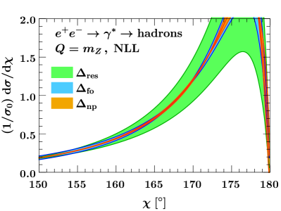
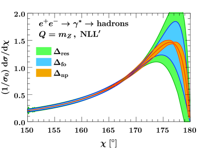
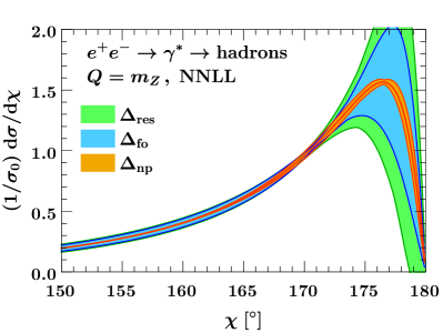
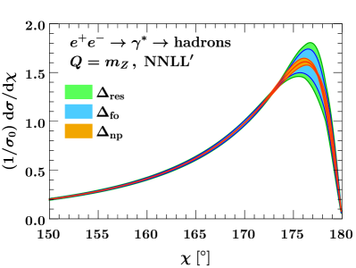
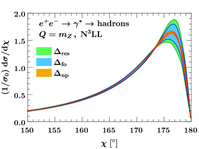
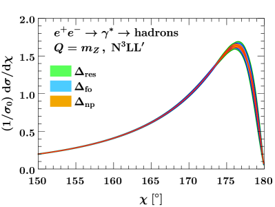
Figure 1: Breakdown of the total uncertainty into fixed-order ($\Delta_{\rm fo}$, blue), resummation ($\Delta_{\rm res}$, green) and nonperturbative ($\Delta_{\rm np}$) uncertainties for different resummation orders.

Figure 2 shows a comparison of the resummed EEC spectrum at various orders. In the left panel, we compare NLL^′ through NNLL^′, while in the right panel we compare NNLL^′ through N³LL^′. In both cases we also plot the nonsingular distribution defined as

$$\frac{\mathrm{d}\sigma^{\text{nons}}}{\mathrm{d}z}\equiv\frac{\mathrm{d}\sigma}{\mathrm{d}z}-\frac{\mathrm{d}\sigma_{1}}{\mathrm{d}z}\,,$$ (67)

where $\mathrm{d}\sigma_{1}/\mathrm{d}z$ is the leading-power cross section in the back-to-back limit as predicted by the factorization formula in eq. (2.1.1) and presented explicitly in section 2.3 up to $\mathcal{O}(\alpha_{s}^{3})$. Thus, $\mathrm{d}\sigma^{\text{nons}}/\mathrm{d}z$ shows the impact of the fixed-order corrections beyond leading power. In the left plot, the dot-dashed black line shows the neglected correction from the NLO fixed-order results calculated in ref. Dixon:2018qgp (with respect to the $\mathcal{O}(\alpha_{s}^{2})$ leading power result), while in the right plot we show the nonsingular distribution at $\mathcal{O}(\alpha_{s}^{3})$ using the NNLO fixed-order results calculated numerically in ref. Tulipant:2017ybb . As expected, these fixed-order corrections are neglibile for $\chi\gtrsim 160^{\circ}$, thus justifying employing canonical leading power resummation in the shown range. One notable feature in figure 2 is that going from NLL^′ to NNLL actually increases the size of the scale variations, except in the region $\chi\sim 170-177^{\circ}$. Nevertheless, the central value at NNNL (blue dashed) is much closer to the central value at NNLL^′ (red solid) than at NLL (green dotted). We observe a similar pattern when comparing NNLL^′ and N³LL in the right panel, even though the effects are less pronounced at this order. Overall, the central values show very good convergence beyond NNLL, with greatly reduced uncertainties at N³LL^′ of about $\pm 4\%$ at the peak, compared to about $\pm 15\%$ at N³LL.

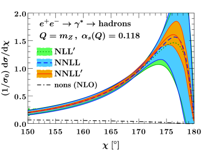
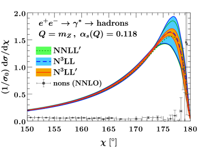
Figure 2: Comparison of the resummed EEC spectrum as a function of the angle $\chi$ at different resummation orders. The shaded areas, bounded by the solid lines, show the individual uncertainties, with the central value indicated according to the legend.

In figure 3, we overlay the N³LL and N³LL^′ resummed spectra of figure 2 with the fixed order NNLO numerical calculation of ref. Tulipant:2017ybb as well as the experimental measurement of the EEC Acton:1993zh from the OPAL collaboration at LEP. We observe that resummation effects improve substantially the behavior of the spectrum in the peak region compared to the fixed order calculation. We also note that pushing the resummation to N³LL^′ accuracy is crucial to achieve a perturbative control on the theory prediction that is competitive with the experimental uncertainty on this observable. However, it is important to point out that for a realistic comparison with experimental data and for the extraction of the strong coupling constant from this event shape, it is essential to include hadronization effects Abreu:1990us ; Acton:1991cu ; Acton:1993zh ; Abreu:1993kj ; Abe:1994mf ; Korchemsky:1999kt ; Tulipant:2017ybb ; Kardos:2018kqj ; dEnterria:2019its , as resummation effects alone, even at N³LL^′, cannot fully bridge the gap between partonic fixed order results and data. For completeness, we also show in figure 3 the analytic leading power spectrum in the back-to-back limit at $\mathcal{O}(\alpha_{s}^{3})$ (in red) from eqs. (2.3.1) and (2.3.1). In the peak region, this result perfectly agrees with the fixed order NNLO numerical calculation of ref. Tulipant:2017ybb , thereby again justifying resummation in this region. Note that the difference between those two results is exactly the non-singular distribution plotted in the right panel of figure 2.

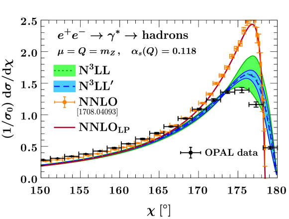
Figure 3: Comparison of the N³LL and N³LL^′ resummed EEC partonic spectrum with the fixed order NNLO numerical calculation of ref. Tulipant:2017ybb , the LEP data from the OPAL collaboration Acton:1993zh , and the analytic leading power spectrum at $\mathcal{O}(\alpha_{s}^{3})$¹² from eq. (2.3.1).

4.4 Comparison to literature

Resummed predictions for the EEC in the back-to-back limit have previously been reported in refs. deFlorian:2004mp ; Tulipant:2017ybb ; Kardos:2018kqj at NNLL, based on the approach developed in refs. Collins:1981uk ; Collins:1981va ; Kodaira:1981nh ; Kodaira:1982az . To compare our formalism to theirs, we start from eq. (4.1) and choose the resummation scales as

$$\mu_{H}=\nu_{J}\equiv\mu_{h}\sim Q\,,\qquad\mu_{J}=\mu_{S}=\nu_{S}\equiv\mu_{l}\sim\frac{b_{0}}{b_{T}}\,,\qquad\mu_{0}=\frac{b_{0}}{b_{T}}\,,$$ (68)

i.e. we distinguish only an overall high scale $\mu_{h}$ and low scale $\mu_{l}$, but always evaluate the rapidity anomalous dimension at its canonical scale $\mu_{0}=b_{0}/b_{T}$. With these choices, eq. (4.1) can be rewritten as

$$\frac{\mathrm{d}\sigma}{\mathrm{d}z} =\frac{\hat{\sigma}_{0}}{8}H_{q{\bar{q}}}(Q,\mu_{h})\int_{0}^{\infty}\!\!\mathrm{d}(b_{T}Q)^{2}\,J_{0}\bigl{(}b_{T}Q\sqrt{1-z}\bigr{)}J_{q}\Bigl{(}b_{T},\mu_{l},\frac{\mu_{h}}{Q}\Bigr{)}J_{\bar{q}}\Bigl{(}b_{T},\mu_{l},\frac{\mu_{h}}{Q}\Bigr{)}\tilde{S}_{q}(b_{T},\mu_{l},\mu_{l})$$

$$\quad\times\exp\left\{-\int_{\mu_{l}^{2}}^{\mu_{h}^{2}}\frac{\mathrm{d}\mu^{\prime 2}}{\mu^{\prime 2}}\left[\ln\frac{Q^{2}}{\mu^{\prime 2}}A^{q}[\alpha_{s}(\mu^{\prime})]+B^{q}[\alpha_{s}(\mu^{\prime})]\right]\right\}$$

$$\quad\times\exp\left\{\ln\frac{\mu_{l}^{2}}{\mu_{h}^{2}}\int_{\mu_{0}^{2}}^{\mu_{l}^{2}}\frac{\mathrm{d}\mu^{\prime 2}}{\mu^{\prime 2}}A^{q}[\alpha_{s}(\mu^{\prime})]+\ln\frac{Q^{2}}{\mu_{h}^{2}}\frac{1}{2}\bigl{[}\tilde{\gamma}_{\nu}^{q}[\alpha_{s}(\mu_{h})]-\tilde{\gamma}_{\nu}^{q}[\alpha_{s}(\mu_{l})]\bigr{]}\right\}\,,$$ (69)

The coefficients $A^{q}$ and $B^{q}$ in eq. (4.4) are given by

$$A^{i}(\alpha_{s}) =\Gamma_{\rm cusp}^{i}(\alpha_{s})+\frac{1}{4}\beta(\alpha_{s})\frac{\mathrm{d}\tilde{\gamma}_{\nu}^{i}(\alpha_{s})}{\mathrm{d}\alpha_{s}}\,,\qquad B^{i}(\alpha_{s})=2\gamma_{i}(\alpha_{s})-\frac{1}{2}\tilde{\gamma}_{\nu}^{i}(\alpha_{s})\,,$$ (70)

where we remind the reader that $\tilde{\gamma}_{\nu}^{i}[\alpha_{s}(b_{0}/b_{T}]\equiv\tilde{\gamma}_{\nu}^{i}(b_{T},b_{0}/b_{T})$ is the boundary term of the rapidity anomalous dimension. Notably, the $A^{q}$ coefficient differs from the cusp anomalous dimension starting at $\mathcal{O}(\alpha_{s}^{3})$, which already contributes at NNLL Becher:2010tm .

In eq. (4.4), the first line contains the fixed-order boundary terms, which at canonical scales are free of any logarithms and only depend on $\alpha_{s}(\mu_{h})=\alpha_{s}(Q)$ and $\alpha_{s}(\mu_{l})=\alpha_{s}(b_{0}/b_{T})$. The second line in eq. (4.4) contains the Sudakov form factor that exponentiates the large logarithms. The third line only contributes when $\mu_{h}\neq Q$ or $\mu_{l}\neq\mu_{0}$, i.e. when scales are not chosen exactly canonically, and thus can be used to assess resummation uncertainties by separately varying $\mu_{h}$ and $\mu_{l}$. We note that this procedure is not quite as refined as the one introduced in section 4.2, where we separately vary all resummation scales. Also note that since $\tilde{\gamma}_{\nu}^{i}=\mathcal{O}(\alpha_{s}^{2})$, the second term in this exponential first contributes at $\mathcal{O}(\alpha_{s}^{3})$.

To compare eq. (4.4) to the results used refs. deFlorian:2004mp ; Tulipant:2017ybb ; Kardos:2018kqj , we now explicitly choose the canonical scales, using which eq. (4.4) reads

$$\frac{\mathrm{d}\sigma}{\mathrm{d}z} =\frac{\hat{\sigma}_{0}}{8}H_{q{\bar{q}}}(Q,\mu_{h})\int_{0}^{\infty}\!\!\mathrm{d}(b_{T}Q)^{2}\,J_{0}\bigl{(}b_{T}Q\sqrt{1-z}\bigr{)}J_{q}\Bigl{(}b_{T},\mu_{l},\frac{\mu_{h}}{Q}\Bigr{)}J_{\bar{q}}\Bigl{(}b_{T},\mu_{l},\frac{\mu_{h}}{Q}\Bigr{)}\tilde{S}_{q}(b_{T},\mu_{l},\mu_{l})$$

$$\qquad\times\exp\left\{-\int_{b_{0}^{2}/b_{T}^{2}}^{Q^{2}}\frac{\mathrm{d}\mu^{\prime 2}}{\mu^{\prime 2}}\left[\ln\frac{Q^{2}}{\mu^{\prime 2}}A^{q}[\alpha_{s}(\mu^{\prime})]+B^{q}[\alpha_{s}(\mu^{\prime})]\right]\right\}\,.$$ (71)

For comparison, the resummation formula given in ref. Tulipant:2017ybb reads

$$\frac{\mathrm{d}\sigma}{\mathrm{d}z} =\frac{\sigma_{\rm tot}}{8}\tilde{H}[\alpha_{s}(\mu_{R})]\int_{0}^{\infty}\mathrm{d}(Qb_{T})^{2}J_{0}\bigl{(}b_{T}Q\sqrt{1-z}\bigr{)}$$

$$\qquad\times\exp\left\{-\int_{b_{0}/b_{T}^{2}}^{Q^{2}}\frac{\mathrm{d}\bar{\mu}^{2}}{\bar{\mu}^{2}}\left[\ln\frac{Q^{2}}{\bar{\mu}^{2}}A^{q}[\alpha_{s}(\bar{\mu})]+B^{q}[\alpha_{s}(\bar{\mu})]\right]\right\}\,,$$ (72)

where $\sigma_{\rm tot}$ is the total hadronic cross section. Comparing eqs. (4.4) and (4.4), we first notice that both formulas contain the same Sudakov form factor. However, as already discussed at the end of section 2.1.1, their result only contains a combined function $\tilde{H}$ instead of separating physics at the high and low scales into a hard function and jet and soft functions, respectively. It obeys

$$\sigma_{\rm tot}\tilde{H}[\alpha_{s}(Q)] =\hat{\sigma}_{0}H_{q{\bar{q}}}[\alpha_{s}(Q)]J_{q}[\alpha_{s}(b_{0}/b_{T})]J_{\bar{q}}[\alpha_{s}(b_{0}/b_{T})]\tilde{S}_{q}[\alpha_{s}(b_{0}/b_{T})]$$

$$\quad\times\bigl{\{}1+\mathcal{O}[\alpha_{s}(Q)]^{2}\bigr{\}}\,.$$ (73)

Here, each term is evaluated at canonical scales, and thus only depends on the scale through the running coupling. Eq. (4.4) is to be understood as a reexpansion in $\alpha_{s}(b_{0}/b_{T})=\alpha_{s}(Q)+\mathcal{O}(\alpha_{s}^{2})$. Due to eq. (4.4), both eqs. (4.4) and (4.4) recover the correct fixed-order expansion of the EEC in the back-to-back limit. However, only eq. (4.4) yields the correct NNLL result, as eq. (4.4) does not contain the correct boundary terms.

As remarked earlier, while the original works in ref. Collins:1981uk ; Collins:1981va ; Kodaira:1981nh ; Kodaira:1982az did not yet contain separate hard and jet functions, as they do not yet contribute a the NLL accuracy they work at, the existence of these functions can already be seen in the $q_{T}$ factorization used in those works to derive the EEC factorization in the back-to-back limit. For instance, ref. Kodaira:1982az also explicitly mentions corrections to the TMDFF in $\alpha_{s}(1/b_{T})$.

Another crucial difference lies in the estimation of perturbative uncertainties. In our approach, we vary all resummation scales, which in particular separately varies the high scale $\mu_{h}\sim Q$ and the low scale $\mu_{l}\sim 1/b_{T}$. This reflects that in the back-to-back limit, the EEC contains two parametrically different scales, and varying both resummation scales probes the physics at both scales. In contrast, in refs. deFlorian:2004mp ; Tulipant:2017ybb ; Kardos:2018kqj effectively only the hard scale $\mu_{R}$ is varied, while the low scale is always kept canonical at $\mu_{l}=\mu_{0}=b_{0}/b_{T}$. This completely neglects the variation from the last line in eq. (4.4), and thus largely underestimates the perturbative uncertainties. Note that due to the lack of a jet and soft function evaluated at the low scale, variations of the low scale can not even cancel formally in eq. (4.4), in contrast to variations of the hard scale $\mu_{R}$. Also note that refs. deFlorian:2004mp ; Tulipant:2017ybb ; Kardos:2018kqj avoid the Landau pole by deforming the integration contour into the complex plane, rather than freezing out the scale as done in our analysis.

The above observation already explains why the perturbative uncertainties observed in our analysis are larger than those seen in refs. deFlorian:2004mp ; Tulipant:2017ybb ; Kardos:2018kqj , as we cover a larger set of scale variations. Moreover, since variations of the low scale $\mu_{l}\sim 1/b_{T}$ probe the strong coupling at much larger values than variations of the high scale $\mu_{h}\sim Q$, it is not surprising that the former are in fact the dominant uncertainties. To validate this, we compare three methods of estimating uncertainties:

1. $\Delta_{\rm tot}$: Full set of profile scale variations as discussed in section 4.2

2. $\Delta(\mu_{h})$: We only consider two variations,

   $$\mu_{H}=\nu_{J}=\frac{1}{2}Q\,,\qquad\mu_{H}=\nu_{J}=2Q\,,$$ (74)

   while all other scales are kept as in eq. (63). This roughly mimics the procedure in refs. deFlorian:2004mp ; Tulipant:2017ybb ; Kardos:2018kqj .

3. $\Delta(\mu_{l})$: We only consider three variations,

   $$(\mu_{J},\mu_{S})=\Bigl{(}\frac{1}{2},1\Bigr{)}\frac{b_{0}}{b_{T}^{*}}\,,\quad(\mu_{J},\mu_{S})=\Bigl{(}1,\frac{1}{2}\Bigr{)}\frac{b_{0}}{b_{T}^{*}}\,,\quad(\mu_{J},\mu_{S})=\Bigl{(}\frac{1}{2},\frac{1}{2}\Bigr{)}\frac{b_{0}}{b_{T}^{*}}\,,$$ (75)

   while all other scales are kept as in eq. (63). These are the only scale variations where the hard scales $\mu_{H,J}$ are unchanged, and the low scales are only varied down. We also keep the rapidity scale $\nu_{S}=b_{0}/b_{T}^{*}$ canonic, as it does not enter the running coupling.

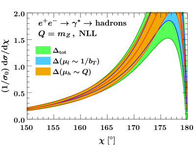
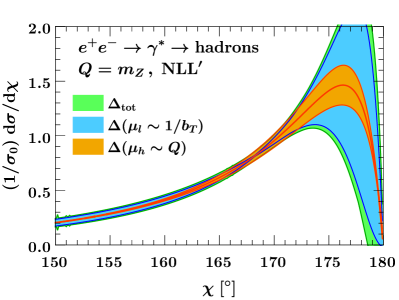
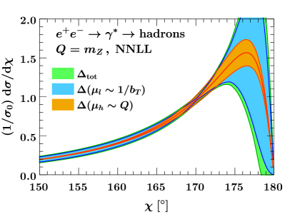
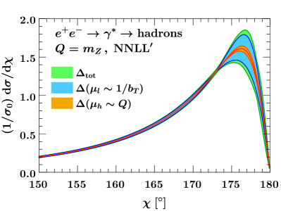
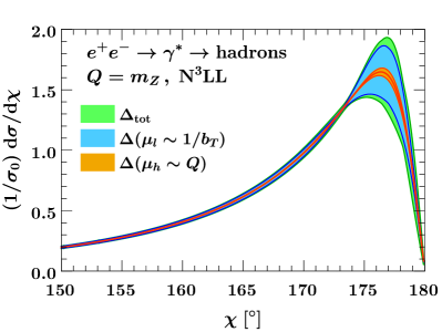
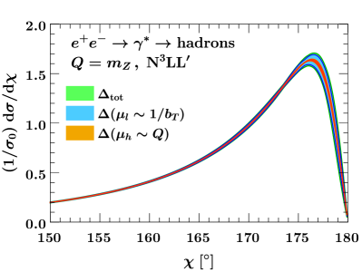
Figure 4: Comparison of the total uncertainty $\Delta_{\rm tot}$, estimated by a full set of profile scale variations, to varying only the high scales $\mu_{h}\sim Q$ or the low scales $\mu_{l}\sim 1/b_{T}$. See text for more details.

The results are shown in figure 4, in a similar pattern as in figure 1 such that one can easily compare the two figures. At NLL, we see that the variations of both the high scale (orange) and low scale (blue) are significant, giving rise to a very large overall uncertainty (green). In contrast, at all higher orders we clearly see that it is indeed the low-scale variation $\Delta(\mu_{l})$ (blue) that dominates the total uncertainty, while the high-scale variation $\Delta(\mu_{h})$ and the remaining scale variations are almost negligible.

In ref. deFlorian:2004mp , the uncertainty of the peak at NNLL was given by roughly $\pm 8\%$, compared to $\Delta(\mu_{h})\sim 12\%$. By only considering the variation $\Delta(\mu_{h})$, our uncertainty at N³LL^′ (N³LL) reduces to only $\pm 0.5\%$ ($\pm 2\%$), compared to our more conservative uncertainty of about $\pm 4\%$ ($\pm 15\%$) when using all scale variations. In both approaches, the uncertainty reduces by a factor of about $4$ when going from N³LL to N³LL^′, illustrating the importance of including the N³LO boundary terms computed in this work. However, we stress again that only varying the high scales neglects important uncertainties from soft physics, and thus the $\Delta(\mu_{h})$ variation alone is not sufficient to obtain a robust estimate of theory uncertainties.

We close by remarking that it was already remarked in ref. Kodaira:1982az that the EEC is quite sensitive to the high $b_{T}$ region, and nonperturbative model functions were introduced in order to achieve agreement with CELLO data. This is consistent with our observation that variations of the $1/b_{T}$ scales yield the dominant uncertainties.

5 Conclusions

In this work we have calculated the full singular structure of the Energy-Energy Correlation (EEC) in the back-to-back limit at $\mathcal{O}(\alpha_{s}^{3})$ in QCD, including contact terms. Our work applies both in the case of $e^{+}e^{-}$ annihilation as well as in gluon induced Higgs decays. To obtain these results we have calculated the quark and gluon jet functions for the EEC in the back-to-back limit at N³LO, which were the last missing ingredients for the factorization theorem in this limit at N³LO.

The computation of the jet functions relies on the calculation of the kernels of the transverse-momentum dependent fragmentation functions at N³LO in our companion paper Ebert:2020qef which have been obtained using a recently developed method for the expansion of cross sections around the collinear limit Ebert:2020lxs . We checked that the logarithmically enhanced terms of our calculation match those predicted by the rapidity renormalization group (RRG) evolution.

By comparing the leading transcendental part of our results we show that the principle of maximal transcendentality, which states that a quantity obtained in $\mathcal{N}=4$ SYM constitutes the leading transcendental term of the same quantity in QCD, holds for the EEC in the back-to-back asymptotic up to $\mathcal{O}(\alpha_{s}^{3})$. In particular, we show that the leading transcendental part of the EEC in $e^{+}e^{-}$ is identical to the one for the EEC in Higgs decay to gluons and that both match the result in $\mathcal{N}=4$ Henn:2019gkr ; Korchemsky:2019nzm ; Kologlu:2019mfz , not only for the logarithmic part but also for the contact terms. This also provides a non-trivial cross check on both the quark and gluon jet function calculations of the $\delta(1-z)$ constants in addition to the one on the logarithmic parts coming from the RRG evolution.

Leveraging on the fact that the EEC obeys a set of non trivial sum rules Korchemsky:2019nzm ; Kologlu:2019mfz , we used our newly calculated result for the contact terms at $\mathcal{O}(\alpha_{s}^{3})$ as well as the logarithmic enhanced contributions in the small angle limit Dixon:2019uzg to obtain the $N=2$ Mellin moment of the EEC distribution in the bulk at NNLO in QCD analytically. This constitutes the first piece of analytic information on the EEC distribution at this order in QCD away from the endpoints, both in the case of $e^{+}e^{-}$ annihilation as well as in gluon induced Higgs decays.

Finally, we have carried out the resummation of the EEC in the back-to-back region at N³LL^′ accuracy. This is the first time an event shape observable is resummed at this level of accuracy and, more generally, this constitutes the highest level of resummation for any infrared and collinear safe observable in QCD to date. We show that by performing the resummation at N³LL^′ we obtain a reduction of uncertainties by a factor of $\sim 4$ in the peak region compared to previous results obtained at lower accuracy. We thoroughly discuss different schemes to estimate the uncertainties due to missing higher order corrections both in the boundary terms as well as in the anomalous dimensions. We compare these different schemes with the ones used in the literature for this observable. Adopting a scheme in line with the ones previously used in the literature we obtain a 5 per-mille uncertainty at the peak. Using a more conservative scheme, which includes a significant contribution from non-perturbative regions, we obtain a 4% uncertainty for our result at N³LL^′. We point out that the accuracy for lower order results is severely affected by the choice of scheme and that varying the low-energy scale gives a dramatically larger estimate of uncertainties.

The recent progress in understanding Energy-Energy correlators is very promising and we believe it shows that they will play a crucial role in improving our understanding of the strong interaction in the years to come. For example, as the EEC has been often used to determine the strong coupling constant Abreu:1990us ; Acton:1991cu ; Abreu:1993kj ; Abe:1994mf ; Tulipant:2017ybb ; Kardos:2018kqj ; dEnterria:2019its , it would be interesting to leverage the high level of perturbative control we gained on this observable thanks to the N³LL^′ resummation, to improve the extraction of $\alpha_{s}$, complementing the extractions based on other event shape observables in $e^{+}e^{-}$ such as thrust and C-parameter Becher:2008cf ; Abbate:2010xh ; Bethke:2011tr ; Hoang:2015hka . In addition, it could also be used to extract nonperturbative corrections to the rapidity anomalous dimensions. We expect that further studies of perturbative Moult:2019vou and non-perturbative Korchemsky:1999kt ; Li:2021txc power corrections will be important to improve the theoretical control on this observable.

It will also be interesting to explore the application of the techniques used in this work and its companion paper Ebert:2020qef to higher point energy correlators in QCD where recent progress has been obtained Chen:2019bpb ; Chen:2020vvp ; Chen:2020adz .

Appendix A Fixed-order structure of the EEC jet function

Here, we provide the fixed-order structure of the jet function, obtained by solving the RG eqs. (2.2) and (2.2) order-by-order in $\alpha_{s}$. The fixed-order coefficients as defined by eq. (21) are given by

$$J_{i}^{(0)}(L_{b},L_{Q}) =1\,,$$

$$J_{i}^{(1)}(L_{b},L_{Q}) =L_{b}\Bigl{(}\Gamma^{i}_{0}L_{Q}+\frac{\tilde{\gamma}^{i}_{J\,0}}{2}\Bigr{)}+j_{i}^{(1)}\,,$$

$$J_{i}^{(2)}(L_{b},L_{Q}) =\frac{1}{2}L_{b}^{2}\Bigl{[}L_{Q}^{2}(\Gamma^{i}_{0})^{2}+\Gamma^{i}_{0}L_{Q}\Bigl{(}\tilde{\gamma}^{i}_{J\,0}+\beta_{0}\Bigr{)}+\frac{1}{4}\tilde{\gamma}^{i}_{J\,0}\Bigl{(}\tilde{\gamma}^{i}_{J\,0}+2\beta_{0}\Bigr{)}\Bigr{]}$$

$$\quad+L_{b}\Bigl{[}L_{Q}\bigl{(}\Gamma^{i}_{1}+\Gamma^{i}_{0}j_{i}^{(1)}\bigr{)}+\frac{1}{2}\tilde{\gamma}^{i}_{J\,1}+\Bigl{(}\frac{1}{2}\tilde{\gamma}^{i}_{J\,0}+\beta_{0}\Bigr{)}j_{i}^{(1)}\Bigr{]}$$

$$\quad-\frac{\tilde{\gamma}^{i}_{\nu\,1}}{2}L_{Q}+j_{i}^{(2)}\,,$$

$$J_{i}^{(3)}(L_{b},L_{Q}) =\frac{1}{6}L_{b}^{3}\Bigl{[}L_{Q}^{3}(\Gamma^{i}_{0})^{3}+\frac{3}{2}(\Gamma^{i}_{0})^{2}L_{Q}^{2}(\tilde{\gamma}^{i}_{J\,0}+2\beta_{0})+\Gamma^{i}_{0}L_{Q}\Bigl{(}\frac{3}{4}(\tilde{\gamma}^{i}_{J\,0})^{2}+3\beta_{0}\tilde{\gamma}^{i}_{J\,0}+2\beta_{0}^{2}\Bigr{)}$$

$$\qquad\quad+\tilde{\gamma}^{i}_{J\,0}\Bigl{(}\frac{3}{4}\beta_{0}\tilde{\gamma}^{i}_{J\,0}+\frac{1}{8}(\tilde{\gamma}^{i}_{J\,0})^{2}+\beta_{0}^{2}\Bigr{)}\Bigr{]}$$

$$\quad+L_{b}^{2}\Bigl{\{}L_{Q}^{2}\Gamma^{i}_{0}\Bigl{(}\Gamma^{i}_{1}+\frac{1}{2}\Gamma^{i}_{0}j_{i}^{(1)}\Bigr{)}$$

$$\qquad\qquad+\frac{1}{2}L_{Q}\Bigl{[}\Gamma^{i}_{1}(\tilde{\gamma}^{i}_{J\,0}+2\beta_{0})+\Gamma^{i}_{0}(\beta_{1}+\tilde{\gamma}^{i}_{J\,1})+\Gamma^{i}_{0}(\tilde{\gamma}^{i}_{J\,0}+3\beta_{0})j_{i}^{(1)}\Bigr{]}$$

$$\qquad\qquad+\frac{1}{2}\beta_{0}\tilde{\gamma}^{i}_{J\,1}+\frac{1}{4}\tilde{\gamma}^{i}_{J\,0}(\tilde{\gamma}^{i}_{J\,1}+\beta_{1})+\Bigl{(}\frac{3}{4}\beta_{0}\tilde{\gamma}^{i}_{J\,0}+\frac{1}{8}(\tilde{\gamma}^{i}_{J\,0})^{2}+\beta_{0}^{2}\Bigr{)}j_{i}^{(1)}\Bigr{\}}$$

$$\quad+L_{b}\Bigl{\{}-\frac{1}{2}\Gamma^{i}_{0}\tilde{\gamma}^{i}_{\nu\,1}L_{Q}^{2}+L_{Q}\Bigl{[}\Gamma^{i}_{2}+\Gamma^{i}_{1}j_{i}^{(1)}+\Gamma^{i}_{0}j_{i}^{(2)}-\Bigl{(}\frac{1}{4}\tilde{\gamma}^{i}_{J\,0}+\beta_{0}\Bigr{)}\tilde{\gamma}^{i}_{\nu\,1}\Bigr{]}$$

$$\qquad\qquad+\frac{1}{2}\tilde{\gamma}^{i}_{J\,2}+\Bigl{(}\frac{1}{2}\tilde{\gamma}^{i}_{J\,1}+\beta_{1}\Bigr{)}j_{i}^{(1)}+\Bigl{(}\frac{1}{2}\tilde{\gamma}^{i}_{J\,0}+2\beta_{0}\Bigr{)}j_{i}^{(2)}\Bigr{\}}$$

$$\quad-\frac{1}{2}L_{Q}\bigl{(}\tilde{\gamma}^{i}_{\nu\,2}+\tilde{\gamma}^{i}_{\nu\,1}j_{i}^{(1)}\bigr{)}+j_{i}^{(3)}\,.$$ (76)

Here, the $\Gamma_{n}^{i}$ and $\gamma_{J\,n}^{i}$ are the $\mathcal{O}[(\alpha_{s}/4\pi)^{n}]$ coefficients of the cusp and jet noncusp anomalous dimensions, respectively, where we remind the reader that the jet noncusp anomalous dimension is identical to that of the TMD beam function, $\gamma_{J\,n}^{i}\equiv\gamma_{B\,n}^{i}$. Explicit expressions for these anomalous dimensions in our conventions are collected in ref. Billis:2019vxg . The corresponding fixed-order expansion of the polarized gluon jet function $J^{\prime}_{g}$ can be obtained from eq. (A) by dropping all terms that do not contain an explicit factor $j_{i}^{(n)}$, as in this case $J_{g}^{\prime(0)}=0$.

Appendix B Bessel transform

To evaluate eqs. (2.1.1) and (2.1.2) at fixed order, we need to evaluate Bessel transforms of the form

$$I_{n} \equiv\frac{1}{8}\int\mathrm{d}(b_{T}^{2}Q^{2})J_{0}\bigl{(}b_{T}Q\sqrt{\bar{z}}\bigr{)}\,\ln^{n}\frac{b_{T}^{2}\mu^{2}}{b_{0}^{2}}$$

$$=\frac{1}{2}\sum_{k=0}^{n-1}(-1)^{k+1}n\binom{n-1}{k}R_{2}^{(n-k-1)}\biggl{[}\frac{\ln^{k}[(Q^{2}/\mu^{2})\bar{z}]}{\bar{z}}\biggr{]}_{+}+\frac{1}{2}R_{2}^{(n)}\delta(\bar{z})\,,$$ (77)

which follows immediately from Eq. (C.16) of ref. Ebert:2016gcn , with

$$R_{2}^{(n)}=\frac{\mathrm{d}^{n}}{\mathrm{d}a^{n}}e^{2\gamma_{E}a}\frac{\Gamma(1+a)}{\Gamma(1-a)}\biggr{|}_{a=0}\,.$$ (78)

The plus distributions in eq. (B) are defined as usual such that $\int_{0}^{1}\mathrm{d}x\,[\ln^{n}x/x]_{+}=0$. They can be easily rewritten in terms of distributions in $\bar{z}$ using

$$\biggl{[}\frac{\ln^{k}[(Q^{2}/\mu^{2})\bar{z}]}{\bar{z}}\biggr{]}_{+} =\sum_{\ell=0}^{k}\binom{k}{\ell}\ln^{\ell}\frac{Q^{2}}{\mu^{2}}\mathcal{L}_{k-\ell}(\bar{z})+\frac{\ln^{k+1}(Q^{2}/\mu^{2})}{k+1}\delta(\bar{z})\,,$$ (79)

where the plus prescription on the right hand side now acts with respect to $\bar{z}$. For example, the first few Bessel transforms read

$$I_{0} =\frac{1}{2}\delta(\bar{z})\,,$$

$$I_{1} =-\frac{1}{2}\bigl{[}\mathcal{L}_{0}(\bar{z})+L_{h}\delta(\bar{z})\bigr{]}\,,$$

$$I_{2} =\mathcal{L}_{1}(\bar{z})+L_{h}\mathcal{L}_{0}(\bar{z})+\frac{1}{2}L_{h}^{2}\delta(\bar{z})\,,$$

$$I_{3} =-\frac{3}{2}\mathcal{L}_{2}(\bar{z})-3L_{h}\mathcal{L}_{1}(\bar{z})-\frac{3}{2}L_{h}^{2}\mathcal{L}_{0}(\bar{z})+\Bigl{(}\frac{1}{2}L_{h}^{3}-2\zeta_{3}\Bigr{)}\delta(\bar{z})\,,$$ (80)

where $L_{h}=\ln(Q^{2}/\mu^{2})$. Starting from $n=3$, the $R_{2}^{(n)}$ terms start to induce $\zeta$ values.

Appendix C Sum Rules Ingredients

Here we collect all required results for the quantities in eq. (48).

First, we note that $V_{1}^{(n)}$ is the coefficient of $\delta(\bar{z})$ at $\mathcal{O}(\alpha_{s}^{n})$, and thus can be immediately read off from the results in eqs. (2.3.1) and (2.3.1) for $e^{+}e^{-}$ and in eqs. (2.3.2) and (2.3.2) for Higgs. For example,

$$V_{1,e^{+}e^{-}}^{(1)}=-C_{F}(4+2\zeta_{2})\,,\qquad V_{1,H}^{(1)}=C_{A}\left(\frac{65}{18}-2\zeta_{2}\right)-\frac{5}{18}n_{f}\,.$$ (81)

The expressions for $V_{0}^{(n)}$, the coefficients of $\delta(z)$, can be in principle extracted via the factorization formula for the EEC in the collinear limit of ref. Dixon:2019uzg . Here, we have extracted them by using the sum rule in eq. (49) and analytically integrating the regular part of the distribution obtained from the fixed order calculation of refs. Dixon:2018qgp ; Luo:2019nig . For $e^{+}e^{-}$ we obtain

$$V_{0}^{(1)} =\frac{13}{24}C_{F}\,,$$

$$V_{0}^{(2)} =C_{F}^{2}\left(44\zeta_{4}-84\zeta_{3}+\frac{109}{12}\zeta_{2}+\frac{208219}{5184}\right)+C_{F}n_{f}\left(\frac{33\zeta_{2}}{20}+4\zeta_{3}-\frac{751777}{216000}\right)$$

$$+C_{F}C_{A}\left(-22\zeta_{4}+36\zeta_{3}-\frac{373}{45}\zeta_{2}-\frac{3032011}{162000}\right)\,,$$ (82)

while for the Higgs case we obtain:

$$V_{0}^{(1)} =\frac{3311}{300}C_{A}-\frac{1447}{600}n_{f}\,,$$

$$V_{0}^{(2)} =C_{A}^{2}\left(22\zeta_{4}-\frac{242}{3}\zeta_{3}-\frac{18337}{450}\zeta_{2}+\frac{31760837}{101250}\right)-C_{A}n_{f}\left(\frac{4}{15}\zeta_{3}-\frac{2891}{225}\zeta_{2}+\frac{183628817}{1620000}\right)$$

$$+C_{F}n_{f}\left(\frac{224}{15}\zeta_{3}-\frac{23}{10}\zeta_{2}-\frac{249491}{12000}\right)-n_{f}^{2}\left(\frac{22}{15}\zeta_{2}-\frac{274091}{27000}\right)$$ (83)

Finally, for the expressions for the total cross section we take the results of ref. Herzog:2017dtz . For $e^{+}e^{-}$ they read

$$R_{e^{+}e^{-}}^{(1)} =3C_{F}$$

$$R_{e^{+}e^{-}}^{(2)} =-{3\over 2}\,\*C_{F}^{2}\,+\,C_{A}\*C_{F}\,\*\Bigg{(}{123\over 2}-44\,\*\zeta_{3}\Bigg{)}\,-\,C_{F}\*n_{f}\,\*\Big{(}11-8\,\*\zeta_{3}\Big{)}$$

$$R_{e^{+}e^{-}}^{(3)} =-{69\over 2}\,\*C_{F}^{3}\,-\,C_{A}\*C_{F}^{2}\,\*\Big{(}127+572\,\*\zeta_{3}-880\,\*\zeta_{5}\Big{)}$$

$$+\,C_{A}^{2}\*C_{F}\,\*\Bigg{(}{90445\over 54}-{242\over 3}\,\*\zeta_{2}-{10948\over 9}\,\*\zeta_{3}-{440\over 3}\,\*\zeta_{5}\Bigg{)}\,-\,C_{F}^{2}\,\*n_{f}\,\*\Bigg{(}{29\over 2}-152\,\*\zeta_{3}+160\,\*\zeta_{5}\Bigg{)}$$

$$-\,C_{A}\*C_{F}\,\*n_{f}\,\*\Bigg{(}{15520\over 27}-{88\over 3}\,\*\zeta_{2}-{3584\over 9}\,\*\zeta_{3}-{80\over 3}\,\*\zeta_{5}\Bigg{)}\,+\,C_{F}\,\*n_{f}^{2}\,\*\Bigg{(}{1208\over 27}-{8\over 3}\,\*\zeta_{2}-{304\over 9}\,\*\zeta_{3}\Bigg{)}\,.$$

$$+N_{F,V}\frac{d_{abc}d^{abc}}{16N_{r}}\left(\frac{176}{3}-128\zeta_{3}\right)\,.$$ (84)

For Higgs, they are given by

$$R_{H}^{(1)} ={73\over 3}\,\*C_{A}-{14\over 3}\,\*n_{f}$$

$$R_{H}^{(2)} =C_{A}^{2}\>\*\Bigg{(}{37631\over 54}-{242\over 3}\,\*\zeta_{2}-110\,\*\zeta_{3}\Bigg{)}\>-\>C_{A}\*\,n_{f}\>\*\Bigg{(}{6665\over 27}-{88\over 3}\,\*\zeta_{2}+4\,\*\zeta_{3}\Bigg{)}$$

$$-\>C_{F}\*\,n_{f}\,\*\Bigg{(}{131\over 3}-24\,\*\zeta_{3}\Bigg{)}\>+\>n_{f}^{2}\>\*\Bigg{(}{508\over 27}-{8\over 3}\,\*\zeta_{2}\Bigg{)}$$

$$R_{H}^{(3)} =C_{A}^{3}\,\*\Bigg{(}\,{15420961\over 729}-{45056\over 9}\,\*\zeta_{2}-{178156\over 27}\,\*\zeta_{3}+{3080\over 3}\,\*\zeta_{5}\Bigg{)}$$

$$-\>C_{A}^{2}\*\,n_{f}\,\*\Bigg{(}\,{2670508\over 243}-{8084\over 3}\,\*\zeta_{2}-{9772\over 9}\,\*\zeta_{3}+{80\over 3}\,\*\zeta_{5}\Bigg{)}$$

$$-\>C_{F}\*C_{A}\*\,n_{f}\,\*\Bigg{(}\,{23221\over 9}-{572\over 3}\,\*\zeta_{2}-1364\,\*\zeta_{3}-160\,\*\zeta_{5}\Bigg{)}$$

$$+\>C_{F}^{2}\*\,n_{f}\,\*\Bigg{(}\,{221\over 3}+192\,\*\zeta_{3}-320\,\*\zeta_{5}\Bigg{)}\>+\>C_{A}\*\,n_{f}^{2}\,\*\Bigg{(}\,{413308\over 243}-{1384\over 3}\,\*\zeta_{2}+{56\over 9}\,\*\zeta_{3}\Bigg{)}\qquad$$

$$+\>C_{F}\*\,n_{f}^{2}\,\*\Big{(}440\>-{104\over 3}\,\*\zeta_{2}-240\,\*\zeta_{3}\Big{)}\>-\>n_{f}^{3}\,\*\Bigg{(}\,{57016\over 729}-{224\over 9}\,\*\zeta_{2}-{64\over 27}\,\*\zeta_{3}\Bigg{)}\,.$$ (85)

References

• (1) C. L. Basham, L. S. Brown, S. D. Ellis and S. T. Love, Energy Correlations in electron - Positron Annihilation: Testing QCD, Phys. Rev. Lett. 41 (1978) 1585.
• (2) DELPHI collaboration, P. Abreu et al., Energy-energy correlations in hadronic final states from Z0 decays, Phys. Lett. B252 (1990) 149.
• (3) OPAL collaboration, P. D. Acton et al., An Improved measurement of $\alpha_{S}(M_{Z^{0}})$ using energy correlations with the OPAL detector at LEP, Phys. Lett. B276 (1992) 547.
• (4) OPAL collaboration, P. D. Acton et al., A Determination of alpha-s (M (Z0)) at LEP using resummed QCD calculations, Z. Phys. C 59 (1993) 1.
• (5) DELPHI collaboration, P. Abreu et al., Determination of $\alpha_{s}$ using the next-to-leading log approximation of QCD, Z. Phys. C59 (1993) 21.
• (6) SLD collaboration, K. Abe et al., Measurement of $\alpha_{s}(M_{Z}^{2})$ from hadronic event observables at the $Z^{0}$ resonance, Phys. Rev. D51 (1995) 962 [hep-ex/9501003].
• (7) Z. Tulipánt, A. Kardos and G. Somogyi, Energy–energy correlation in electron–positron annihilation at NNLL + NNLO accuracy, Eur. Phys. J. C 77 (2017) 749 [1708.04093].
• (8) A. Kardos, S. Kluth, G. Somogyi, Z. Tulipánt and A. Verbytskyi, Precise determination of $\alpha_{S}(M_{Z})$ from a global fit of energy–energy correlation to NNLO+NNLL predictions, Eur. Phys. J. C 78 (2018) 498 [1804.09146].
• (9) SISSA, $\alpha_{s}$(2019): Precision measurements of the QCD coupling, vol. ALPHAS2019, SISSA, 2019.
• (10) V. Del Duca, C. Duhr, A. Kardos, G. Somogyi and Z. Trócsányi, Three-Jet Production in Electron-Positron Collisions at Next-to-Next-to-Leading Order Accuracy, Phys. Rev. Lett. 117 (2016) 152004 [1603.08927].
• (11) G. Somogyi, Z. Trocsanyi and V. Del Duca, A Subtraction scheme for computing QCD jet cross sections at NNLO: Regularization of doubly-real emissions, JHEP 01 (2007) 070 [hep-ph/0609042].
• (12) G. Somogyi and Z. Trocsanyi, A Subtraction scheme for computing QCD jet cross sections at NNLO: Regularization of real-virtual emission, JHEP 01 (2007) 052 [hep-ph/0609043].
• (13) U. Aglietti, V. Del Duca, C. Duhr, G. Somogyi and Z. Trocsanyi, Analytic integration of real-virtual counterterms in NNLO jet cross sections. I., JHEP 09 (2008) 107 [0807.0514].
• (14) L. J. Dixon, M.-X. Luo, V. Shtabovenko, T.-Z. Yang and H. X. Zhu, Analytical Computation of Energy-Energy Correlation at Next-to-Leading Order in QCD, Phys. Rev. Lett. 120 (2018) 102001 [1801.03219].
• (15) M.-X. Luo, V. Shtabovenko, T.-Z. Yang and H. X. Zhu, Analytic Next-To-Leading Order Calculation of Energy-Energy Correlation in Gluon-Initiated Higgs Decays, JHEP 06 (2019) 037 [1903.07277].
• (16) A. V. Belitsky, S. Hohenegger, G. P. Korchemsky, E. Sokatchev and A. Zhiboedov, From correlation functions to event shapes, Nucl. Phys. B884 (2014) 305 [1309.0769].
• (17) A. V. Belitsky, S. Hohenegger, G. P. Korchemsky, E. Sokatchev and A. Zhiboedov, Event shapes in $\mathcal{N}=4$ super-Yang-Mills theory, Nucl. Phys. B884 (2014) 206 [1309.1424].
• (18) A. V. Belitsky, S. Hohenegger, G. P. Korchemsky, E. Sokatchev and A. Zhiboedov, Energy-Energy Correlations in N=4 Supersymmetric Yang-Mills Theory, Phys. Rev. Lett. 112 (2014) 071601 [1311.6800].
• (19) J. M. Henn, E. Sokatchev, K. Yan and A. Zhiboedov, Energy-energy correlation in $N$=4 super Yang-Mills theory at next-to-next-to-leading order, Phys. Rev. D100 (2019) 036010 [1903.05314].
• (20) J. M. Maldacena, The Large N limit of superconformal field theories and supergravity, Int. J. Theor. Phys. 38 (1999) 1113 [hep-th/9711200].
• (21) D. M. Hofman and J. Maldacena, Conformal collider physics: Energy and charge correlations, JHEP 05 (2008) 012 [0803.1467].
• (22) I. Moult, G. Vita and K. Yan, Subleading power resummation of rapidity logarithms: the energy-energy correlator in $\mathcal{N}$ = 4 SYM, JHEP 07 (2020) 005 [1912.02188].
• (23) G. P. Korchemsky, Energy correlations in the end-point region, JHEP 01 (2020) 008 [1905.01444].
• (24) L. J. Dixon, I. Moult and H. X. Zhu, Collinear limit of the energy-energy correlator, Phys. Rev. D100 (2019) 014009 [1905.01310].
• (25) D. Chicherin, J. M. Henn, E. Sokatchev and K. Yan, From correlation functions to event shapes in QCD, JHEP 02 (2021) 053 [2001.10806].
• (26) J. M. Henn, What can we learn about QCD and collider physics from N=4 super Yang-Mills?, 2006.00361.
• (27) H. Chen, T.-Z. Yang, H. X. Zhu and Y. J. Zhu, Analytic Continuation and Reciprocity Relation for Collinear Splitting in QCD, Chin. Phys. C45 (2021) 043101 [2006.10534].
• (28) H. Chen, I. Moult and H. X. Zhu, Quantum Interference in Jet Substructure from Spinning Gluons, Phys. Rev. Lett. 126 (2021) 112003 [2011.02492].
• (29) A. Ali, E. Pietarinen and W. Stirling, Transverse Energy-energy Correlations: A Test of Perturbative QCD for the Proton - Anti-proton Collider, Phys. Lett. B 141 (1984) 447.
• (30) A. Gao, H. T. Li, I. Moult and H. X. Zhu, Precision QCD Event Shapes at Hadron Colliders: The Transverse Energy-Energy Correlator in the Back-to-Back Limit, Phys. Rev. Lett. 123 (2019) 062001 [1901.04497].
• (31) H. T. Li, I. Vitev and Y. J. Zhu, Transverse-Energy-Energy Correlations in Deep Inelastic Scattering, JHEP 11 (2020) 051 [2006.02437].
• (32) A. Ali, G. Li, W. Wang and Z.-P. Xing, Transverse energy–energy correlations of jets in the electron–proton deep inelastic scattering at HERA, Eur. Phys. J. C80 (2020) 1096 [2008.00271].
• (33) E. Remiddi and J. A. M. Vermaseren, Harmonic polylogarithms, Int. J. Mod. Phys. A15 (2000) 725 [hep-ph/9905237].
• (34) K. Konishi, A. Ukawa and G. Veneziano, On the Transverse Spread of QCD Jets, Phys. Lett. B 80 (1979) 259.
• (35) D. de Florian and M. Grazzini, The Back-to-back region in e+ e- energy-energy correlation, Nucl. Phys. B 704 (2005) 387 [hep-ph/0407241].
• (36) J. C. Collins and D. E. Soper, Back-To-Back Jets in QCD, Nucl. Phys. B193 (1981) 381.
• (37) J. C. Collins and D. E. Soper, Back-To-Back Jets: Fourier Transform from B to K-Transverse, Nucl. Phys. B197 (1982) 446.
• (38) J. Kodaira and L. Trentadue, Summing Soft Emission in QCD, Phys. Lett. B 112 (1982) 66.
• (39) J. Kodaira and L. Trentadue, Single Logarithm Effects in electron-Positron Annihilation, Phys. Lett. B 123 (1983) 335.
• (40) I. Moult and H. X. Zhu, Simplicity from Recoil: The Three-Loop Soft Function and Factorization for the Energy-Energy Correlation, JHEP 08 (2018) 160 [1801.02627].
• (41) M. Kologlu, P. Kravchuk, D. Simmons-Duffin and A. Zhiboedov, The light-ray OPE and conformal colliders, JHEP 01 (2021) 128 [1905.01311].
• (42) M. A. Ebert, B. Mistlberger and G. Vita, TMD Fragmentation Functions at N3LO, 2012.07853.
• (43) M.-x. Luo, T.-Z. Yang, H. X. Zhu and Y. J. Zhu, Unpolarized Quark and Gluon TMD PDFs and FFs at N3LO, 2012.03256.
• (44) C. W. Bauer, S. Fleming and M. E. Luke, Summing Sudakov logarithms in $B\to X_{s}\gamma$ in effective field theory, Phys. Rev. D63 (2000) 014006 [hep-ph/0005275].
• (45) C. W. Bauer, S. Fleming, D. Pirjol and I. W. Stewart, An Effective field theory for collinear and soft gluons: Heavy to light decays, Phys. Rev. D63 (2001) 114020 [hep-ph/0011336].
• (46) C. W. Bauer and I. W. Stewart, Invariant operators in collinear effective theory, Phys. Lett. B516 (2001) 134 [hep-ph/0107001].
• (47) C. W. Bauer, D. Pirjol and I. W. Stewart, Soft collinear factorization in effective field theory, Phys. Rev. D65 (2002) 054022 [hep-ph/0109045].
• (48) J. Collins, Foundations of perturbative QCD, vol. 32. Cambridge University Press, 11, 2013.
• (49) J. C. Collins and A. Metz, Universality of soft and collinear factors in hard-scattering factorization, Phys. Rev. Lett. 93 (2004) 252001 [hep-ph/0408249].
• (50) Y. J. Zhu, Double soft current at one-loop in QCD, 2009.08919.
• (51) M. A. Ebert, B. Mistlberger and G. Vita, Transverse momentum dependent PDFs at N3LO, JHEP 09 (2020) 146 [2006.05329].
• (52) I. Feige, D. W. Kolodrubetz, I. Moult and I. W. Stewart, A Complete Basis of Helicity Operators for Subleading Factorization, JHEP 11 (2017) 142 [1703.03411].
• (53) I. Moult, I. W. Stewart and G. Vita, A subleading operator basis and matching for gg → H, JHEP 07 (2017) 067 [1703.03408].
• (54) M. A. Ebert, I. Moult, I. W. Stewart, F. J. Tackmann, G. Vita and H. X. Zhu, Subleading power rapidity divergences and power corrections for qT, JHEP 04 (2019) 123 [1812.08189].
• (55) I. Moult, M. P. Solon, I. W. Stewart and G. Vita, Fermionic Glauber Operators and Quark Reggeization, JHEP 02 (2018) 134 [1709.09174].
• (56) G. P. Korchemsky and G. F. Sterman, Power corrections to event shapes and factorization, Nucl. Phys. B 555 (1999) 335 [hep-ph/9902341].
• (57) H. T. Li, Y. Makris and I. Vitev, Energy-energy correlators in Deep Inelastic Scattering, Phys. Rev. D 103 (2021) 094005 [2102.05669].
• (58) J.-Y. Chiu, A. Jain, D. Neill and I. Z. Rothstein, A Formalism for the Systematic Treatment of Rapidity Logarithms in Quantum Field Theory, JHEP 05 (2012) 084 [1202.0814].
• (59) T. Becher, M. Neubert and D. Wilhelm, Higgs-Boson Production at Small Transverse Momentum, JHEP 05 (2013) 110 [1212.2621].
• (60) M. G. Echevarria, T. Kasemets, P. J. Mulders and C. Pisano, QCD evolution of (un)polarized gluon TMDPDFs and the Higgs $q_{T}$-distribution, JHEP 07 (2015) 158 [1502.05354].
• (61) M.-X. Luo, X. Wang, X. Xu, L. L. Yang, T.-Z. Yang and H. X. Zhu, Transverse Parton Distribution and Fragmentation Functions at NNLO: the Quark Case, JHEP 10 (2019) 083 [1908.03831].
• (62) M. A. Ebert, B. Mistlberger and G. Vita, Collinear expansion for color singlet cross sections, JHEP 09 (2020) 181 [2006.03055].
• (63) Y. Li, D. Neill and H. X. Zhu, An exponential regulator for rapidity divergences, Nucl. Phys. B960 (2020) 115193 [1604.00392].
• (64) Y. Li and H. X. Zhu, Bootstrapping Rapidity Anomalous Dimensions for Transverse-Momentum Resummation, Phys. Rev. Lett. 118 (2017) 022004 [1604.01404].
• (65) G. Billis, M. A. Ebert, J. K. L. Michel and F. J. Tackmann, A toolbox for $q_{T}$ and 0-jettiness subtractions at $\hbox{N}^{3}\hbox{LO}$, Eur. Phys. J. Plus 136 (2021) 214 [1909.00811].
• (66) M.-X. Luo, T.-Z. Yang, H. X. Zhu and Y. J. Zhu, Transverse Parton Distribution and Fragmentation Functions at NNLO: the Gluon Case, JHEP 01 (2020) 040 [1909.13820].
• (67) T. Gehrmann, E. W. N. Glover, T. Huber, N. Ikizlerli and C. Studerus, Calculation of the quark and gluon form factors to three loops in QCD, JHEP 06 (2010) 094 [1004.3653].
• (68) G. P. Korchemsky and A. V. Radyushkin, Renormalization of the Wilson Loops Beyond the Leading Order, Nucl. Phys. B283 (1987) 342.
• (69) Z. Bern, L. J. Dixon and V. A. Smirnov, Iteration of planar amplitudes in maximally supersymmetric Yang-Mills theory at three loops and beyond, Phys. Rev. D 72 (2005) 085001 [hep-th/0505205].
• (70) J. M. Henn, G. P. Korchemsky and B. Mistlberger, The full four-loop cusp anomalous dimension in $\mathcal{N}=4$ super Yang-Mills and QCD, JHEP 04 (2020) 018 [1911.10174].
• (71) L. J. Dixon, L. Magnea and G. F. Sterman, Universal structure of subleading infrared poles in gauge theory amplitudes, JHEP 08 (2008) 022 [0805.3515].
• (72) L. J. Dixon, The Principle of Maximal Transcendentality and the Four-Loop Collinear Anomalous Dimension, JHEP 01 (2018) 075 [1712.07274].
• (73) B. Eden, Three-loop universal structure constants in N=4 susy Yang-Mills theory, 1207.3112.
• (74) L. F. Alday and A. Bissi, Higher-spin correlators, JHEP 10 (2013) 202 [1305.4604].
• (75) P. Baikov, K. Chetyrkin, J. Kuhn and J. Rittinger, Complete ${\cal O}(\alpha_{s}^{4})$ QCD Corrections to Hadronic $Z$-Decays, Phys. Rev. Lett. 108 (2012) 222003 [1201.5804].
• (76) P. Baikov, K. Chetyrkin, J. Kuhn and J. Rittinger, Adler Function, Sum Rules and Crewther Relation of Order ${\cal O}(\alpha_{s}^{4})$: the Singlet Case, Phys. Lett. B 714 (2012) 62 [1206.1288].
• (77) F. Herzog, B. Ruijl, T. Ueda, J. Vermaseren and A. Vogt, On Higgs decays to hadrons and the R-ratio at N4LO, JHEP 08 (2017) 113 [1707.01044].
• (78) M. A. Ebert, I. W. Stewart and Y. Zhao, Determining the Nonperturbative Collins-Soper Kernel From Lattice QCD, Phys. Rev. D99 (2019) 034505 [1811.00026].
• (79) M. A. Ebert, I. W. Stewart and Y. Zhao, Towards Quasi-Transverse Momentum Dependent PDFs Computable on the Lattice, JHEP 09 (2019) 037 [1901.03685].
• (80) A. A. Vladimirov and A. Schäfer, Transverse momentum dependent factorization for lattice observables, Phys. Rev. D101 (2020) 074517 [2002.07527].
• (81) P. Shanahan, M. Wagman and Y. Zhao, Collins-Soper kernel for TMD evolution from lattice QCD, Phys. Rev. D 102 (2020) 014511 [2003.06063].
• (82) Lattice Parton collaboration, Q.-A. Zhang et al., Lattice QCD Calculations of Transverse-Momentum-Dependent Soft Function through Large-Momentum Effective Theory, Phys. Rev. Lett. 125 (2020) 192001 [2005.14572].
• (83) A. A. Vladimirov, Self-contained definition of the Collins-Soper kernel, Phys. Rev. Lett. 125 (2020) 192002 [2003.02288].
• (84) G. Bell, A. Hornig, C. Lee and J. Talbert, $e^{+}e^{-}$ angularity distributions at NNLL accuracy, JHEP 01 (2019) 147 [1808.07867].
• (85) G. Billis, F. J. Tackmann and J. Talbert, Higher-Order Sudakov Resummation in Coupled Gauge Theories, JHEP 03 (2020) 182 [1907.02971].
• (86) L. G. Almeida, S. D. Ellis, C. Lee, G. Sterman, I. Sung and J. R. Walsh, Comparing and counting logs in direct and effective methods of QCD resummation, JHEP 04 (2014) 174 [1401.4460].
• (87) G. Kramer and B. Lampe, Two Jet Cross-Section in $e^{+}e^{-}$ Annihilation, Z. Phys. C34 (1987) 497.
• (88) T. Matsuura and W. L. van Neerven, Second Order Logarithmic Corrections to the Drell-Yan Cross-section, Z. Phys. C38 (1988) 623.
• (89) T. Matsuura, S. C. van der Marck and W. L. van Neerven, The Calculation of the Second Order Soft and Virtual Contributions to the Drell-Yan Cross-Section, Nucl. Phys. B319 (1989) 570.
• (90) T. Gehrmann, T. Huber and D. Maitre, Two-loop quark and gluon form-factors in dimensional regularisation, Phys. Lett. B622 (2005) 295 [hep-ph/0507061].
• (91) S. Moch, J. A. M. Vermaseren and A. Vogt, Three-loop results for quark and gluon form-factors, Phys. Lett. B625 (2005) 245 [hep-ph/0508055].
• (92) S. Moch, J. A. M. Vermaseren and A. Vogt, The Quark form-factor at higher orders, JHEP 08 (2005) 049 [hep-ph/0507039].
• (93) P. A. Baikov, K. G. Chetyrkin, A. V. Smirnov, V. A. Smirnov and M. Steinhauser, Quark and gluon form factors to three loops, Phys. Rev. Lett. 102 (2009) 212002 [0902.3519].
• (94) R. N. Lee, A. V. Smirnov and V. A. Smirnov, Analytic Results for Massless Three-Loop Form Factors, JHEP 04 (2010) 020 [1001.2887].
• (95) S. Moch, J. A. M. Vermaseren and A. Vogt, The Three loop splitting functions in QCD: The Nonsinglet case, Nucl. Phys. B688 (2004) 101 [hep-ph/0403192].
• (96) A. Vogt, S. Moch and J. A. M. Vermaseren, The Three-loop splitting functions in QCD: The Singlet case, Nucl. Phys. B691 (2004) 129 [hep-ph/0404111].
• (97) J. Henn, A. V. Smirnov, V. A. Smirnov, M. Steinhauser and R. N. Lee, Four-loop photon quark form factor and cusp anomalous dimension in the large-$N_{c}$ limit of QCD, JHEP 03 (2017) 139 [1612.04389].
• (98) S. Moch, B. Ruijl, T. Ueda, J. Vermaseren and A. Vogt, Four-Loop Non-Singlet Splitting Functions in the Planar Limit and Beyond, JHEP 10 (2017) 041 [1707.08315].
• (99) R. N. Lee, A. V. Smirnov, V. A. Smirnov and M. Steinhauser, Four-loop quark form factor with quartic fundamental colour factor, JHEP 02 (2019) 172 [1901.02898].
• (100) J. Henn, T. Peraro, M. Stahlhofen and P. Wasser, Matter dependence of the four-loop cusp anomalous dimension, Phys. Rev. Lett. 122 (2019) 201602 [1901.03693].
• (101) R. Brüser, A. Grozin, J. M. Henn and M. Stahlhofen, Matter dependence of the four-loop QCD cusp anomalous dimension: from small angles to all angles, JHEP 05 (2019) 186 [1902.05076].
• (102) A. von Manteuffel, E. Panzer and R. M. Schabinger, Cusp and collinear anomalous dimensions in four-loop QCD from form factors, Phys. Rev. Lett. 124 (2020) 162001 [2002.04617].
• (103) R. V. Harlander, Virtual corrections to $gg\to H$ to two loops in the heavy top limit, Phys. Lett. B492 (2000) 74 [hep-ph/0007289].
• (104) I. W. Stewart, F. J. Tackmann and W. J. Waalewijn, The Quark Beam Function at NNLL, JHEP 09 (2010) 005 [1002.2213].
• (105) C. F. Berger, C. Marcantonini, I. W. Stewart, F. J. Tackmann and W. J. Waalewijn, Higgs Production with a Central Jet Veto at NNLL+NNLO, JHEP 04 (2011) 092 [1012.4480].
• (106) R. Brüser, Z. L. Liu and M. Stahlhofen, Three-Loop Quark Jet Function, Phys. Rev. Lett. 121 (2018) 072003 [1804.09722].
• (107) P. Banerjee, P. K. Dhani and V. Ravindran, Gluon jet function at three loops in QCD, Phys. Rev. D98 (2018) 094016 [1805.02637].
• (108) M.-x. Luo, T.-Z. Yang, H. X. Zhu and Y. J. Zhu, Quark Transverse Parton Distribution at the Next-to-Next-to-Next-to-Leading Order, Phys. Rev. Lett. 124 (2020) 092001 [1912.05778].
• (109) T. Lübbert, J. Oredsson and M. Stahlhofen, Rapidity renormalized TMD soft and beam functions at two loops, JHEP 03 (2016) 168 [1602.01829].
• (110) A. A. Vladimirov, Correspondence between Soft and Rapidity Anomalous Dimensions, Phys. Rev. Lett. 118 (2017) 062001 [1610.05791].
• (111) O. V. Tarasov, A. A. Vladimirov and A. Yu. Zharkov, The Gell-Mann-Low Function of QCD in the Three Loop Approximation, Phys. Lett. 93B (1980) 429.
• (112) S. A. Larin and J. A. M. Vermaseren, The Three loop QCD Beta function and anomalous dimensions, Phys. Lett. B303 (1993) 334 [hep-ph/9302208].
• (113) T. van Ritbergen, J. A. M. Vermaseren and S. A. Larin, The Four loop beta function in quantum chromodynamics, Phys. Lett. B400 (1997) 379 [hep-ph/9701390].
• (114) M. Czakon, The Four-loop QCD beta-function and anomalous dimensions, Nucl. Phys. B710 (2005) 485 [hep-ph/0411261].
• (115) M. A. Ebert, J. K. L. Michel and F. J. Tackmann, Resummation Improved Rapidity Spectrum for Gluon Fusion Higgs Production, JHEP 05 (2017) 088 [1702.00794].
• (116) G. Lustermans, J. K. Michel, F. J. Tackmann and W. J. Waalewijn, Joint two-dimensional resummation in $q_{T}$ and 00-jettiness at NNLL, JHEP 03 (2019) 124 [1901.03331].
• (117) I. W. Stewart, F. J. Tackmann, J. R. Walsh and S. Zuberi, Jet $p_{T}$ resummation in Higgs production at $NNLL^{\prime}+NNLO$, Phys. Rev. D 89 (2014) 054001 [1307.1808].
• (118) M. A. Ebert, J. K. L. Michel, F. J. Tackmann et al., SCETlib: A C++ Package for Numerical Calculations in QCD and Soft-Collinear Effective Theory, DESY-17-099 (2018) .
• (119) T. Becher and M. Neubert, Drell-Yan Production at Small $q_{T}$, Transverse Parton Distributions and the Collinear Anomaly, Eur. Phys. J. C71 (2011) 1665 [1007.4005].
• (120) T. Becher and M. D. Schwartz, A precise determination of $\alpha_{s}$ from LEP thrust data using effective field theory, JHEP 07 (2008) 034 [0803.0342].
• (121) R. Abbate, M. Fickinger, A. H. Hoang, V. Mateu and I. W. Stewart, Thrust at $N^{3}LL$ with Power Corrections and a Precision Global Fit for $\alpha_{s}(mZ)$, Phys. Rev. D 83 (2011) 074021 [1006.3080].
• (122) S. Bethke et al., Workshop on Precision Measurements of $\alpha_{s}$, 1110.0016.
• (123) A. H. Hoang, D. W. Kolodrubetz, V. Mateu and I. W. Stewart, Precise determination of $\alpha_{s}$ from the $C$-parameter distribution, Phys. Rev. D91 (2015) 094018 [1501.04111].
• (124) H. Chen, M.-X. Luo, I. Moult, T.-Z. Yang, X. Zhang and H. X. Zhu, Three point energy correlators in the collinear limit: symmetries, dualities and analytic results, JHEP 08 (2020) 028 [1912.11050].
• (125) H. Chen, I. Moult, X. Zhang and H. X. Zhu, Rethinking jets with energy correlators: Tracks, resummation, and analytic continuation, Phys. Rev. D 102 (2020) 054012 [2004.11381].
• (126) M. A. Ebert and F. J. Tackmann, Resummation of Transverse Momentum Distributions in Distribution Space, JHEP 02 (2017) 110 [1611.08610].