The Liouville line element and the energy of the diagonals

Abstract.

In this work I show that in each rectangle formed by the parameter curves on a Liouville surface the energies of the main diagonals are equal. This result extends naturally to $n$-dimensional Liouville manifolds.

1. Introduction

In this work I show that in each rectangle formed by the parameter lines on a Liouville surface the diagonals have the same energy (see the main theorem 2.6). This is valid, when the surface has what I call an orthogonal Liouville line element (including all special cases, like the isothermal one for $U_{2}=U_{1}$ and $V_{2}=V_{1}$ which is known as Liouville line element in the literature) of the form:

$${\mathop{}\!\textnormal{d}s}^{2}=(U_{1}(u)+V_{1}(v)){\mathop{}\!\textnormal{d}u}^{2}+(U_{2}(u)+V_{2}(v)){\mathop{}\!\textnormal{d}v}^{2}$$

The diagonals are, in general, not geodesics on the surface; they are the image curves of the diagonals in a rectangle formed by two pairs of parameter lines in the definition domain. If the line element is isothermal then the parametrization of the surface is conformal and preserves angles between curves and therefore the diagonals on the surface are isogonal trajectories with respect to the parameter curves of the surface.

1.1. Plane isothermal Liouville maps

In the plane there are only four distinct isothermal Liouville maps (up to similarity transforms), see figure 1.1.

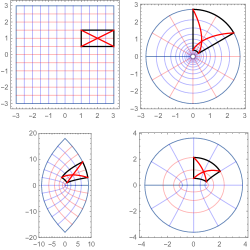
Figure 1.1. Isothermal Liouville coordinates on the plane: the two diagonals in each rectangle have the same energy

The diagonals of each rectangle formed by parameter lines in the domain of definition are mapped to isogonal trajectories with respect to the parameter lines in the image plane because the map is isothermal and therefore conformal, see figure 1.1.

Because the line element of these maps is isothermal Liouville, the diagonals in each rectangle formed by pairs of parameter lines (belonging each to the two different families of parameter lines) have the same energy (see theorem 2.4 for the proof).

If we take the straight line diagonals – these are geodesics in the plane – then we have the theorem of Ivory:

Theorem 1.1 (Ivory).

The geodesic diagonals in a rectangle formed by parameter lines have the same length if and only if the map has a Stäckel line element.

Remark 1.2.

This theorem was proved by W. Blaschke [3] and his student K. Zwirner [17] for the $2$ and $3$ dimensional case and it is valid in higher dimensions too. A proof is also found in [10] and [8] where they say that A. Thimm filled a gap in W. Blaschke’s proof.

The isothermal Liouville map is of Stäckel type and therefore the straight line diagonals have the same length, see figure 1.2.

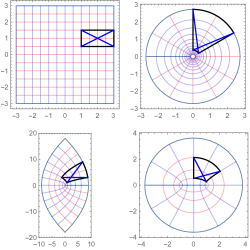
Figure 1.2. Isothermal Liouville coordinates on the plane: the two (straight line) geodesic diagonals in each rectangle have the same length, according to Ivory’s theorem

If we take a parameter line rectangle in one of the four isothermal Liouville coordinates, then we can prove a statement about the energies of the discrete diagonals of the rectangle, in the sense of discrete differential geometry. We take the common interval of definition of the diagonals and partition it uniformly in $k$ pieces. Then we construct polygons approximating the diagonals. We can show that for each $k\in\mathbb{N}$ the two polygons have the same energy, see figure 1.3.

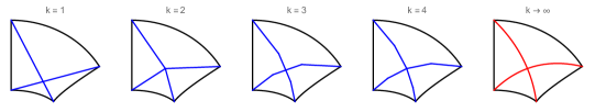
Figure 1.3. For each $k$ the two (discrete) diagonals have the same energy

Here $k=1$ corresponds to the theorem of Ivory in the plane because the two diagonals are geodesics and then their length and energy are related by the Schwarz inequality. They not only have the same energy (the energy of a segment equals the squared length) in this case, but also the same length.

The limiting case $k\to\infty$ corresponds to the main theorem 2.6 of this work. All this can be viewed as a generalization of Ivory’s theorem (see [1]).

1.2. Plane orthogonal Liouville maps

An example for a plane orthogonal Liouville map in $U_{1}(u)$ and $V_{2}(v)$ which is also of Stäckel type can be seen in figure 1.4.

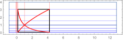
Figure 1.4. Orthogonal Liouville map

The statement about the energies of the discrete diagonals also holds in this case, see figure 1.5.

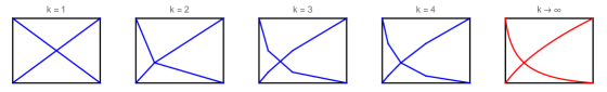
Figure 1.5. For each $k$ the two (discrete) diagonals have the same energy

For $k=1$ we have the theorem of Ivory and for each value of $k$ the two diagonals have the same energy. The generalization of Ivory’s theorem is valid in this case.

I conjecture that this generalization of Ivory’s theorem also holds in parameter line rectangles on Liouville surfaces. Instead of straight lines, there we have to consider polygons formed with segments of geodesics on the surface.

2. Energy of the diagonals

2.1. Definitions

The length $L(p)$ and the energy $E(p)$ of a curve $p:[a,b]\rightarrow M$ in a Riemannian manifold $M$ are given by the following expressions (see [6], (Chapter 9, p. 194)) and they are related by the Schwarz inequality (with equality if and only if $\left|\dot{p}(t)\right|$ is constant, that means $p(t)$ is parametrized proportionally to arc length):

$$L(p) =\int_{a}^{b}{\left|\dot{p}(t)\right|}{\mathop{}\!\textnormal{d}t}=\int_{a}^{b}{\sqrt{\dot{p}(t)\cdot\dot{p}(t)}}{\mathop{}\!\textnormal{d}t}$$

$$E(p) =\int_{a}^{b}{\left|\dot{p}(t)\right|^{2}}{\mathop{}\!\textnormal{d}t}=\int_{a}^{b}{\dot{p}(t)\cdot\dot{p}(t)}{\mathop{}\!\textnormal{d}t}$$

$$L^{2}(p) \leq(b-a)E(p)$$

where $\dot{p}(t)$ is the tangent vector of the curve and $\_\cdot\_$ is the scalar product in $TM$.

Remark 2.1.

Let’s assume that $\left|\dot{p}(t)\right|=q=\text{const.}$ Then we have:

$$L^{2}(p)=\left(\int_{a}^{b}q{\mathop{}\!\textnormal{d}t}\right)^{2}=(b-a)^{2}q^{2}=(b-a)\int_{a}^{b}q^{2}{\mathop{}\!\textnormal{d}t}=(b-a)E(p)$$

The length and energy have the expressions:

$$L(p)=(b-a)q\quad\text{and}\quad E(p)=(b-a)q^{2}$$

If $0<q<1$ then $L(p)>E(p)$. If $1<q$ then $L(p)<E(p)$.

For an arc length parametrized geodesic $\left|\dot{\gamma}(t)\right|=q=1$ we have equality:

$$L(\gamma)=(b-a)=E(\gamma)$$

Thus the geodesic $\gamma(t)$ is (at the same time!) energy and length minimizing.

If the manifold $M$ is the Euclidean plane, we can construct a discretization as follows: we partition the interval $[a,b]$ uniformly in $m$ pieces:

$$a<a+1\frac{b-a}{m}<a+2\frac{b-a}{m}<\cdots<a+(m-1)\frac{b-a}{m}<b$$

The discrete length is then given by:

$$L(p,m)=\sum_{k=1}^{m}\left|p\left(a+k\frac{b-a}{m}\right)-p\left(a+(k-1)\frac{b-a}{m}\right)\right|$$

By taking a limit for $m\to\infty$ we get:

$$\lim_{m\to\infty}L(p,m) =\lim_{m\to\infty}\sum_{k=1}^{m}\frac{\left|p\left(a+k\frac{b-a}{m}\right)-p\left(a+(k-1)\frac{b-a}{m}\right)\right|}{\frac{b-a}{m}}\cdot\frac{b-a}{m}$$

$$=\lim_{m\to\infty}\sum_{k=1}^{m}\left|\frac{p\left(t_{k-1}+\Delta t\right)-p\left(t_{k-1}\right)}{\Delta t}\right|\cdot\Delta t=\int_{a}^{b}{\left|\dot{p}(t)\right|}{\mathop{}\!\textnormal{d}t}=L(p)$$

The discrete energy is given by:

$$E(p,m)=\sum_{k=1}^{m}\frac{\left(p\left(a+k\frac{b-a}{m}\right)-p\left(a+(k-1)\frac{b-a}{m}\right)\right)^{2}}{\frac{b-a}{m}}$$

By taking a limit for $m\to\infty$ we get:

$$\lim_{m\to\infty}E(p,m) =\lim_{m\to\infty}\sum_{k=1}^{m}\left(\frac{p\left(a+k\frac{b-a}{m}\right)-p\left(a+(k-1)\frac{b-a}{m}\right)}{\frac{b-a}{m}}\right)^{2}\cdot\frac{b-a}{m}$$

$$=\lim_{m\to\infty}\sum_{k=1}^{m}\left(\frac{p\left(t_{k-1}+\Delta t\right)-p\left(t_{k-1}\right)}{\Delta t}\right)^{2}\cdot\Delta t=\int_{a}^{b}{\left|\dot{p}(t)\right|^{2}}{\mathop{}\!\textnormal{d}t}=E(p)$$

This way we see that the discrete length and energy are consistent with the length and energy defined at the beginning of this section.

Let’s compute the length $L$ and energy $E$ of a curve $p(t)$ on a surface $S$ with parametrization ${\bf x}(u,v)$.

The curve is given by $p(t)={\bf x}(u(t),v(t)):[a,b]\stackrel{{\scriptstyle c}}{{\rightarrow}}\mathbb{R}^{2}\stackrel{{\scriptstyle{\bf x}}}{{\rightarrow}}S\subset\mathbb{R}^{n}$ (here $n\in\{2,3\}$). First we compute $\dot{p}(t)$:

$$\dot{p}(t)={\bf x}_{u}(u(t),v(t))\dot{u}(t)+{\bf x}_{v}(u(t),v(t))\dot{v}(t)$$

The scalar product $\dot{p}(t)\cdot\dot{p}(t)$ with itself is:

$$\dot{p}(t)\cdot\dot{p}(t) ={\bf x}_{u}(u(t),v(t))\cdot{\bf x}_{u}(u(t),v(t))(\dot{u}(t))^{2}$$

$$+2{\bf x}_{u}(u(t),v(t))\cdot{\bf x}_{v}(u(t),v(t))\dot{u}(t)\dot{v}(t)$$

$$+{\bf x}_{v}(u(t),v(t))\cdot{\bf x}_{v}(u(t),v(t))(\dot{v}(t))^{2}$$

Now we see the connection with the metric tensor (line element) of $S$:

$$\dot{p}(t)\cdot\dot{p}(t)=g_{11}(u(t),v(t))(\dot{u}(t))^{2}+2g_{12}(u(t),v(t))\dot{u}(t)\dot{v}(t)+g_{22}(u(t),v(t))(\dot{v}(t))^{2}$$

With $c(t)=\begin{pmatrix}u(t),v(t)\end{pmatrix}^{t}$ and the matrix $G(c(t))$ of the metric tensor, we can write:

$$\dot{p}(t)\cdot\dot{p}(t)=\dot{c}(t)^{t}G(c(t))\dot{c}(t)=\begin{pmatrix}\dot{u}(t),\dot{v}(t)\end{pmatrix}\begin{pmatrix}g_{11}(u(t),v(t))&g_{12}(u(t),v(t))\\ g_{21}(u(t),v(t))&g_{22}(u(t),v(t))\end{pmatrix}\begin{pmatrix}\dot{u}(t)\\ \dot{v}(t)\end{pmatrix}$$

Now we can define the length and energy of a curve on a surface:

Definition 2.2 (Length of a curve on a surface).

The length of a curve $p(t)={\bf x}(c(t))$ on the surface ${\bf x}(u,v)$ is given by:

$$L({\bf x}(c(t)))=\int_{a}^{b}\sqrt{\dot{c}(t)^{t}G(c(t))\dot{c}(t)}{\mathop{}\!\textnormal{d}t}$$

Definition 2.3 (Energy of a curve on a surface).

The energy of a curve $p(t)={\bf x}(c(t))$ on the surface ${\bf x}(u,v)$ is given by:

$$E({\bf x}(c(t)))=\int_{a}^{b}\dot{c}(t)^{t}G(c(t))\dot{c}(t){\mathop{}\!\textnormal{d}t}$$

2.2. Main theorem

Here we prove two theorems which together give the main theorem 2.6 of this work:

Theorem 2.4.

If a surface ${\bf x}(u,v)$ has the following orthogonal Liouville line element:

$${\mathop{}\!\textnormal{d}s}^{2}=(U_{1}(u)+V_{1}(v)){\mathop{}\!\textnormal{d}u}^{2}+(U_{2}(u)+V_{2}(v)){\mathop{}\!\textnormal{d}v}^{2}$$

then the diagonals in each rectangle formed by parameter lines on the surface have the same energy.

Proof.

We proceed in several steps:

1. We construct a rectangle $ABCD$ in the parameter domain $\left]u_{min},u_{max}\right[\times\left]v_{min},v_{max}\right[$ of the surface ${\bf x}(u,v)$. First we take a point $M=(u_{0},v_{0})^{t}$ as the center of the rectangle. Second, we use a vector $\delta=(\alpha,\beta)^{t}$ (with $\alpha\leq 0$, $\beta\leq 0$) and set $A=M+\delta$. Then the first diagonal $CA$ of rectangle $ABCD$ has the parametrization $d_{1}(t)=M+t\delta$ with $t\in[-1,1]$: for $t=-1$ we get the point $C$, for $t=0$ the point $M$ and for $t=1$ the point $A$. For the second diagonal we use the vector ${\overline{\delta}}=(-\alpha,\beta)^{t}$. The second diagonal $DB$ of rectangle $ABCD$ has the parametrization $d_{2}(t)=M+t{\overline{\delta}}$ with $t\in[-1,1]$: for $t=-1$ we get the point $D$, for $t=0$ the point $M$ and for $t=1$ the point $B$. In choosing $M$ and $\delta$, we must be careful to ensure that $M$, $A$ and $C$ stay inside the definition domain $\left]u_{min},u_{max}\right[\times\left]v_{min},v_{max}\right[$. Then the sides of this rectangle $ABCD$ are parameter lines in the definition domain.

2. For the diagonals on the surface we have:

   $$q_{1}(t) =\dot{d_{1}}(t)^{t}G(d_{1}(t))\dot{d_{1}}(t)$$

   $$=\begin{pmatrix}\alpha,\beta\end{pmatrix}\begin{pmatrix}U_{1}(u_{0}+t\alpha)+V_{1}(v_{0}+t\beta)&0\\ 0&U_{2}(u_{0}+t\alpha)+V_{2}(v_{0}+t\beta)\end{pmatrix}\begin{pmatrix}\alpha\\ \beta\end{pmatrix}$$

   $$=\alpha^{2}(U_{1}(u_{0}+t\alpha)+V_{1}(v_{0}+t\beta))+\beta^{2}(U_{2}(u_{0}+t\alpha)+V_{2}(v_{0}+t\beta))$$

   and

   $$q_{2}(t) =\dot{d_{2}}(t)^{t}G(d_{2}(t))\dot{d_{2}}(t)$$

   $$=\begin{pmatrix}-\alpha,\beta\end{pmatrix}\begin{pmatrix}U_{1}(u_{0}-t\alpha)+V_{1}(v_{0}+t\beta)&0\\ 0&U_{2}(u_{0}-t\alpha)+V_{2}(v_{0}+t\beta)\end{pmatrix}\begin{pmatrix}-\alpha\\ \beta\end{pmatrix}$$

   $$=\alpha^{2}(U_{1}(u_{0}-t\alpha)+V_{1}(v_{0}+t\beta))+\beta^{2}(U_{2}(u_{0}-t\alpha)+V_{2}(v_{0}+t\beta))$$

3. We show that the function $f(t)=q_{1}(t)-q_{2}(t)$ is an odd function of $t$, that means $f(-t)=-f(t)$:

   $$f(-t)= q_{1}(-t)-q_{2}(-t)$$

   $$= \alpha^{2}(U_{1}(u_{0}-t\alpha)+V_{1}(v_{0}-t\beta))+\beta^{2}(U_{2}(u_{0}-t\alpha)+V_{2}(v_{0}-t\beta))$$

   $$-\alpha^{2}(U_{1}(u_{0}+t\alpha)+V_{1}(v_{0}-t\beta))-\beta^{2}(U_{2}(u_{0}+t\alpha)+V_{2}(v_{0}-t\beta))$$

   $$= \alpha^{2}U_{1}(u_{0}-t\alpha)+\beta^{2}U_{2}(u_{0}-t\alpha)-\alpha^{2}U_{1}(u_{0}+t\alpha)-\beta^{2}U_{2}(u_{0}+t\alpha)$$

   $$= \alpha^{2}(U_{1}(u_{0}-t\alpha)+V_{1}(v_{0}+t\beta))+\beta^{2}(U_{2}(u_{0}-t\alpha)+V_{2}(v_{0}+t\beta))$$

   $$-\alpha^{2}(U_{1}(u_{0}+t\alpha)+V_{1}(v_{0}+t\beta))+\beta^{2}(U_{2}(u_{0}+t\alpha)+V_{2}(v_{0}+t\beta))$$

   $$= q_{2}(t)-q_{1}(t)=-f(t)$$

4. For the energies of the diagonals ${\bf x}(d_{1}(t))$ and ${\bf x}(d_{2}(t))$ on the surface we have:

   $$E({\bf x}(d_{1}(t)))-E({\bf x}(d_{2}(t))) =\int_{-1}^{+1}q_{1}(t){\mathop{}\!\textnormal{d}t}-\int_{-1}^{+1}q_{2}(t){\mathop{}\!\textnormal{d}t}$$

   $$=\int_{-1}^{+1}q_{1}(t)-q_{2}(t){\mathop{}\!\textnormal{d}t}=\int_{-1}^{+1}f(t){\mathop{}\!\textnormal{d}t}=0$$

We see that $E({\bf x}(d_{1}(t)))=E({\bf x}(d_{2}(t)))$ and we are done. ∎

Theorem 2.5.

If the diagonals in each rectangle formed by parameter lines on a surface ${\bf x}(u,v)$ have the same energy, then the surface has the following orthogonal Liouville line element:

$${\mathop{}\!\textnormal{d}s}^{2}=(U_{1}(u)+V_{1}(v)){\mathop{}\!\textnormal{d}u}^{2}+(U_{2}(u)+V_{2}(v)){\mathop{}\!\textnormal{d}v}^{2}$$

Proof.

We need several steps:

1. We construct a square $A_{1}B_{1}C_{1}D_{1}$ in the parameter domain $\left]u_{min},u_{max}\right[\times\left]v_{min},v_{max}\right[$ of the surface ${\bf x}(u,v)$. First we take the point $M=(u_{0},v_{0})^{t}$ as the center of the square. Second, we use a vector $\delta=(\alpha,\alpha)^{t}$ (with $\alpha<0$) and set $A_{1}=M+\delta$. Then the first diagonal $C_{1}A_{1}$ of the square $A_{1}B_{1}C_{1}D_{1}$ has the parametrization $d_{1}(t)=M+t\delta$ with $t\in[-1,1]$. For the second diagonal we use the vector ${\overline{\delta}}=(-\alpha,\alpha)^{t}$. The second diagonal $D_{1}B_{1}$ of square $A_{1}B_{1}C_{1}D_{1}$ has the parametrization $d_{2}(t)=M+t{\overline{\delta}}$ with $t\in[-1,1]$. In choosing $M$ and $\delta$, we must be careful to ensure that $M$, $A_{1}$ and $C_{1}$ stay inside the definition domain $\left]u_{min},u_{max}\right[\times\left]v_{min},v_{max}\right[$. Then the sides of this square $A_{1}B_{1}C_{1}D_{1}$ are parameter lines in the definition domain.

2. The metric tensor of the surface has the general form:

   $$G(u,v)=\begin{pmatrix}g_{11}(u,v)&g_{12}(u,v)\\ g_{12}(u,v)&g_{22}(u,v)\end{pmatrix}$$

   and we compute $q_{1}(t)$ and $q_{2}(t)$:

   $$q_{1}(t) =\dot{d_{1}}(t)^{t}G(d_{1}(t))\dot{d_{1}}(t)$$

   $$=\begin{pmatrix}\alpha,\alpha\end{pmatrix}\begin{pmatrix}g_{11}(u_{0}+t\alpha,v_{0}+t\alpha)&g_{12}(u_{0}+t\alpha,v_{0}+t\alpha)\\ g_{12}(u_{0}+t\alpha,v_{0}+t\alpha)&g_{22}(u_{0}+t\alpha,v_{0}+t\alpha)\end{pmatrix}\begin{pmatrix}\alpha\\ \alpha\end{pmatrix}$$

   $$=\alpha^{2}(g_{11}(u_{0}+t\alpha,v_{0}+t\alpha)+2g_{12}(u_{0}+t\alpha,v_{0}+t\alpha)+g_{22}(u_{0}+t\alpha,v_{0}+t\alpha))$$

   and

   $$q_{2}(t) =\dot{d_{2}}(t)^{t}G(d_{2}(t))\dot{d_{2}}(t)$$

   $$=\begin{pmatrix}-\alpha,\alpha\end{pmatrix}\begin{pmatrix}g_{11}(u_{0}-t\alpha,v_{0}+t\alpha)&g_{12}(u_{0}-t\alpha,v_{0}+t\alpha)\\ g_{12}(u_{0}-t\alpha,v_{0}+t\alpha)&g_{22}(u_{0}-t\alpha,v_{0}+t\alpha)\end{pmatrix}\begin{pmatrix}-\alpha\\ \alpha\end{pmatrix}$$

   $$=\alpha^{2}(g_{11}(u_{0}-t\alpha,v_{0}+t\alpha)-2g_{12}(u_{0}-t\alpha,v_{0}+t\alpha)+g_{22}(u_{0}-t\alpha,v_{0}+t\alpha))$$

3. We know that the energies of the diagonals are equal and this implies that the function $f_{1}(t)=q_{1}(t)-q_{2}(t)$ is odd. Then the expression $f_{1}(-t)+f_{1}(t)=0$ is the constant zero function. For the particular value $t=0$, $f_{1}(0)=q_{1}(0)-q_{2}(0)=0$.

   $$0=f_{1}(0)= \alpha^{2}(g_{11}(u_{0},v_{0})+2g_{12}(u_{0},v_{0})+g_{22}(u_{0},v_{0}))$$

   $$-\alpha^{2}(g_{11}(u_{0},v_{0})-2g_{12}(u_{0},v_{0})+g_{22}(u_{0},v_{0}))=4\alpha^{2}g_{12}(u_{0},v_{0})$$

   Therefore $g_{12}(u_{0},v_{0})=0$ on the whole domain of definition, because $\alpha\neq 0$ and we can choose the point $(u_{0},v_{0})^{t}$ freely on the domain of definition. In what follows, we will use $g_{12}(u,v)=0$ (the line element is orthogonal).

4. For $f_{1}(t)$ we now have (with $g_{12}(u,v)=0$):

   $$f_{1}(t)= \alpha^{2}(g_{11}(u_{0}+t\alpha,v_{0}+t\alpha)+g_{22}(u_{0}+t\alpha,v_{0}+t\alpha)$$

   $$-g_{11}(u_{0}-t\alpha,v_{0}+t\alpha)-g_{22}(u_{0}-t\alpha,v_{0}+t\alpha))$$

   And we know that $c_{1}(t):=f_{1}(-t)+f_{1}(t)=0$ is the constant zero function:

   $$f_{1}(-t)+f_{1}(t)= \alpha^{2}(g_{11}(u_{0}-t\alpha,v_{0}-t\alpha)+g_{22}(u_{0}-t\alpha,v_{0}-t\alpha)$$

   $$-g_{11}(u_{0}+t\alpha,v_{0}-t\alpha)-g_{22}(u_{0}+t\alpha,v_{0}-t\alpha))$$

   $$+\alpha^{2}(g_{11}(u_{0}+t\alpha,v_{0}+t\alpha)+g_{22}(u_{0}+t\alpha,v_{0}+t\alpha)$$

   $$-g_{11}(u_{0}-t\alpha,v_{0}+t\alpha)-g_{22}(u_{0}-t\alpha,v_{0}+t\alpha))$$

   Therefore also the derivative $\frac{{\mathop{}\!\textnormal{d}c_{1}}(t)}{\mathop{}\!\textnormal{d}t}=0$ with respect to $t$ is the constant zero function. We can take another derivative $\frac{\mathop{}\!\textnormal{d}^{2}c_{1}(t)}{\mathop{}\!\textnormal{d}t^{2}}=0$ and know that it still is the constant zero function for all values of $t$. For $t=0$ we get

   $$0=\frac{\mathop{}\!\textnormal{d}^{2}c_{1}(0)}{\mathop{}\!\textnormal{d}t^{2}}=8\alpha^{4}\left(\frac{\partial^{2}g_{11}\left(u_{0},v_{0}\right)}{\partial u\,\partial v}+\frac{\partial^{2}g_{22}\left(u_{0},v_{0}\right)}{\partial u\,\partial v}\right)$$

   Because $\alpha\neq 0$ we have the following relation between $g_{11}(u,v)$ and $g_{22}(u,v)$:

   $$\frac{\partial^{2}g_{22}\left(u,v\right)}{\partial u\,\partial v}=-\frac{\partial^{2}g_{11}\left(u,v\right)}{\partial u\,\partial v}$$ (2.1)

5. We construct a rectangle $A_{2}B_{2}C_{2}D_{2}$ in the parameter domain $\left]u_{min},u_{max}\right[\times\left]v_{min},v_{max}\right[$ of the surface ${\bf x}(u,v)$. First we take the point $M=(u_{0},v_{0})^{t}$ as the center of the rectangle. Second, we use a vector $\delta=(\alpha,\alpha\varepsilon)^{t}$ (with $\alpha<0$, $0<\varepsilon<1$) and set $A_{2}=M+\delta$. Then the first diagonal $C_{2}A_{2}$ of rectangle $A_{2}B_{2}C_{2}D_{2}$ has the parametrization $d_{3}(t)=M+t\delta$ with $t\in[-1,1]$. For the second diagonal we use the vector ${\overline{\delta}}=(-\alpha,\alpha\varepsilon)^{t}$. The second diagonal $D_{2}B_{2}$ of rectangle $A_{2}B_{2}C_{2}D_{2}$ has the parametrization $d_{4}(t)=M+t{\overline{\delta}}$ with $t\in[-1,1]$. In choosing $M$ and $\delta$, we must be careful to ensure that $M$, $A_{2}$ and $C_{2}$ stay inside the definition domain $\left]u_{min},u_{max}\right[\times\left]v_{min},v_{max}\right[$. Then the sides of this rectangle $A_{2}B_{2}C_{2}D_{2}$ are parameter lines in the definition domain.

6. The metric tensor of the surface has the form (remember that $g_{12}(u,v)=0$):

   $$G(u,v)=\begin{pmatrix}g_{11}(u,v)&0\\ 0&g_{22}(u,v)\end{pmatrix}$$

   and we compute $q_{3}(t)$ and $q_{4}(t)$:

   $$q_{3}(t) =\dot{d_{3}}(t)^{t}G(d_{3}(t))\dot{d_{3}}(t)$$

   $$=\begin{pmatrix}\alpha,\alpha\varepsilon\end{pmatrix}\begin{pmatrix}g_{11}(u_{0}+t\alpha,v_{0}+t\alpha\varepsilon)&0\\ 0&g_{22}(u_{0}+t\alpha,v_{0}+t\alpha\varepsilon)\end{pmatrix}\begin{pmatrix}\alpha\\ \alpha\varepsilon\end{pmatrix}$$

   $$=\alpha^{2}(g_{11}(u_{0}+t\alpha,v_{0}+t\alpha\varepsilon)+\varepsilon^{2}g_{22}(u_{0}+t\alpha,v_{0}+t\alpha\varepsilon))$$

   and

   $$q_{4}(t) =\dot{d_{4}}(t)^{t}G(d_{4}(t))\dot{d_{4}}(t)$$

   $$=\begin{pmatrix}-\alpha,\alpha\varepsilon\end{pmatrix}\begin{pmatrix}g_{11}(u_{0}-t\alpha,v_{0}+t\alpha\varepsilon)&0\\ 0&g_{22}(u_{0}-t\alpha,v_{0}+t\alpha\varepsilon)\end{pmatrix}\begin{pmatrix}-\alpha\\ \alpha\varepsilon\end{pmatrix}$$

   $$=\alpha^{2}(g_{11}(u_{0}-t\alpha,v_{0}+t\alpha\varepsilon)+\varepsilon^{2}g_{22}(u_{0}-t\alpha,v_{0}+t\alpha\varepsilon))$$

7. We know that the energies of the diagonals are equal and this implies that the function $f_{2}(t)=q_{3}(t)-q_{4}(t)$ is odd. Then the expression $f_{2}(-t)+f_{2}(t)=0$ is the constant zero function.

8. For $f_{2}(t)$ we have:

   $$f_{2}(t)= \alpha^{2}(g_{11}(u_{0}+t\alpha,v_{0}+t\alpha\varepsilon)+\varepsilon^{2}g_{22}(u_{0}+t\alpha,v_{0}+t\alpha\varepsilon))$$

   $$-\alpha^{2}(g_{11}(u_{0}-t\alpha,v_{0}+t\alpha\varepsilon)+\varepsilon^{2}g_{22}(u_{0}-t\alpha,v_{0}+t\alpha\varepsilon))$$

   And we know that $c_{2}(t):=f_{2}(-t)+f_{2}(t)=0$.

   $$c_{2}(t)= \alpha^{2}(\varepsilon^{2}g_{22}\left(u_{0}-t\alpha,v_{0}-t\alpha\varepsilon\right)-\varepsilon^{2}g_{22}\left(u_{0}-t\alpha,v_{0}+t\alpha\varepsilon\right)$$

   $$-\varepsilon^{2}g_{22}\left(u_{0}+t\alpha,v_{0}-t\alpha\varepsilon\right)+\varepsilon^{2}g_{22}\left(u_{0}+t\alpha,v_{0}+t\alpha\varepsilon\right)$$

   $$+g_{11}\left(u_{0}-t\alpha,v_{0}-t\alpha\varepsilon\right)-g_{11}\left(u_{0}-t\alpha,v_{0}+t\alpha\varepsilon\right)$$

   $$-g_{11}\left(u_{0}+t\alpha,v_{0}-t\alpha\varepsilon\right)+g_{11}\left(u_{0}+t\alpha,v_{0}+t\alpha\varepsilon\right))$$

   Therefore also the derivative $\frac{{\mathop{}\!\textnormal{d}c_{2}}(t)}{\mathop{}\!\textnormal{d}t}=0$ with respect to $t$ is the constant zero function. We can take another derivative $\frac{\mathop{}\!\textnormal{d}^{2}c_{2}(t)}{\mathop{}\!\textnormal{d}t^{2}}=0$ and know that it still is the constant zero function for all values of $t$. We use relation (2.1) and we get for $t=0$:

   $$0=\frac{\mathop{}\!\textnormal{d}^{2}c_{2}(0)}{\mathop{}\!\textnormal{d}t^{2}}=8\alpha^{4}\varepsilon\left(1-\varepsilon^{2}\right)\frac{\partial^{2}g_{11}\left(u_{0},v_{0}\right)}{\partial u\,\partial v}$$

   Because $\alpha\neq 0$ and $0<\varepsilon<1$ we have (combined with (2.1)):

   $$\frac{\partial^{2}g_{11}\left(u,v\right)}{\partial u\,\partial v}=0\quad\text{and}\quad\frac{\partial^{2}g_{22}\left(u,v\right)}{\partial u\,\partial v}=0$$

9. By solving each of these differential equations separately with respect to $u$ and $v$ we get:

   $$g_{11}(u,v)=U_{1}(u)+V_{1}(v)\quad\text{and}\quad g_{22}(u,v)=U_{2}(u)+V_{2}(v)$$

And we are done. ∎

The previous two theorems combined give together the following main theorem of this work:

Theorem 2.6 (Main theorem).

If and only if a surface ${\bf x}(u,v)$ has the following orthogonal Liouville line element:

$${\mathop{}\!\textnormal{d}s}^{2}=(U_{1}(u)+V_{1}(v)){\mathop{}\!\textnormal{d}u}^{2}+(U_{2}(u)+V_{2}(v)){\mathop{}\!\textnormal{d}v}^{2}$$

the diagonals in each rectangle formed by parameter lines on the surface have the same energy.

Corollary 2.7.

It immediately follows that for all special cases of this line element the diagonals have the same energy.

3. Liouville surfaces

In this section we define and name some special line elements or parametrizations of surfaces and give examples of Liouville surfaces.

3.1. Definitions

Let a surface be given as a parametrization ${\bf x}(u,v):\left]u_{min},u_{max}\right[\times\left]v_{min},v_{max}\right[\subset\mathbb{R}^{2}\mapsto\mathbb{R}^{n}$ (in this work we have $n\in\{2,3\}$ but the theory is valid in any dimension).

Definition 3.1 (Line element and first fundamental form).

We define the line element ${\mathop{}\!\textnormal{d}s}$ of the surface ${\bf x}(u,v)$ by the first fundamental form $ds^{2}$:

$${\mathop{}\!\textnormal{d}s}^{2}=g_{11}(u,v){\mathop{}\!\textnormal{d}u}^{2}+2g_{12}(u,v){\mathop{}\!\textnormal{d}u}{\mathop{}\!\textnormal{d}v}+g_{22}(u,v){\mathop{}\!\textnormal{d}v}^{2}$$ (3.1)

where $g_{11}(u,v)={\bf x}_{u}(u,v)\boldsymbol{\cdot}{\bf x}_{u}(u,v)$, $g_{12}(u,v)=g_{21}(u,v)={\bf x}_{u}(u,v)\boldsymbol{\cdot}{\bf x}_{v}(u,v)$ and $g_{22}(u,v)={\bf x}_{v}(u,v)\boldsymbol{\cdot}{\bf x}_{v}(u,v)$.

When $g_{12}=0$, the $u$-lines $v=\rm const.$ and $v$-lines $u=\rm const.$ are orthogonal to each other on the surface and we speak of an orthogonal parametrization:

Definition 3.2 (Orthogonal parametrization).

When the line element ${\mathop{}\!\textnormal{d}s}$ of the surface ${\bf x}(u,v)$ has the following form:

$${\mathop{}\!\textnormal{d}s}^{2}=g_{11}(u,v){\mathop{}\!\textnormal{d}u}^{2}+g_{22}(u,v){\mathop{}\!\textnormal{d}v}^{2}$$ (3.2)

with $g_{12}(u,v)=g_{21}(u,v)=0$, the parametrization of the surface is called orthogonal.

When $g_{11}=g_{22}$, $g_{12}=0$ the parametrization is orthogonal and locally conformal (preserves angles between curves (their tangent vectors)):

Definition 3.3 (Isothermal (or conformal) parametrization).

When the line element ${\mathop{}\!\textnormal{d}s}$ of the surface ${\bf x}(u,v)$ has the following form:

$${\mathop{}\!\textnormal{d}s}^{2}=g_{11}(u,v)({\mathop{}\!\textnormal{d}u}^{2}+{\mathop{}\!\textnormal{d}v}^{2})$$ (3.3)

with $g_{11}(u,v)=g_{22}(u,v)$ and $g_{12}(u,v)=g_{21}(u,v)=0$, the parametrization of the surface is called isothermal.

Now we can define Liouville and Clairaut parametrizations:

Definition 3.4 (Orthogonal Liouville parametrization).

When the line element ${\mathop{}\!\textnormal{d}s}$ of the surface ${\bf x}(u,v)$ has the following form:

$${\mathop{}\!\textnormal{d}s}^{2}=(U_{1}(u)+V_{1}(v)){\mathop{}\!\textnormal{d}u}^{2}+(U_{2}(u)+V_{2}(v)){\mathop{}\!\textnormal{d}v}^{2}$$ (3.4)

with $\frac{\partial^{2}}{\partial u\partial v}g_{11}(u,v)=\frac{\partial^{2}}{\partial u\partial v}g_{22}(u,v)=0$ and $g_{12}(u,v)=g_{21}(u,v)=0$, the parametrization of the surface is called orthogonal Liouville parametrization.

A special case is (when $g_{11}=g_{22}$):

Definition 3.5 (Isothermal (or classical) Liouville parametrization).

When the line element ${\mathop{}\!\textnormal{d}s}$ of the surface ${\bf x}(u,v)$ has the following form:

$${\mathop{}\!\textnormal{d}s}^{2}=(U(u)+V(v))({\mathop{}\!\textnormal{d}u}^{2}+{\mathop{}\!\textnormal{d}v}^{2})$$ (3.5)

with $g_{11}(u,v)=g_{22}(u,v)=U(u)+V(v)$ and $g_{12}(u,v)=g_{21}(u,v)=0$, the parametrization of the surface is called isothermal Liouville parametrization.

The Liouville parametrizations specialize further to Clairaut parametrizations, when $g_{11}$ and $g_{22}$ depend only on $u$ (or on $v$):

Definition 3.6 (Orthogonal Clairaut parametrization in $u$).

When the line element ${\mathop{}\!\textnormal{d}s}$ of the surface ${\bf x}(u,v)$ has the following form:

$${\mathop{}\!\textnormal{d}s}^{2}=U_{1}(u){\mathop{}\!\textnormal{d}u}^{2}+U_{2}(u){\mathop{}\!\textnormal{d}v}^{2}$$ (3.6)

with $\frac{\partial}{\partial v}g_{11}(u,v)=\frac{\partial}{\partial v}g_{22}(u,v)=0$ and $g_{12}(u,v)=g_{21}(u,v)=0$, the parametrization of the surface is called orthogonal Clairaut parametrization in $u$. (The other case is that of the orthogonal Clairaut parametrization in $v$.)

A special case is (when $g_{11}=g_{22}=U(u)$ or $g_{11}=g_{22}=V(v)$):

Definition 3.7 (Isothermal Clairaut parametrization in $u$).

When the line element ${\mathop{}\!\textnormal{d}s}$ of the surface ${\bf x}(u,v)$ has the following form:

$${\mathop{}\!\textnormal{d}s}^{2}=U(u)({\mathop{}\!\textnormal{d}u}^{2}+{\mathop{}\!\textnormal{d}v}^{2})$$ (3.7)

with $g_{11}(u,v)=g_{22}(u,v)=U(u)$ and $g_{12}(u,v)=g_{21}(u,v)=0$, the parametrization of the surface is called isothermal Clairaut parametrization in $u$. (The other case is that of the isothermal Clairaut parametrization in $v$.)

Other two special cases worth mentioning are:

Definition 3.8 (Orthogonal Liouville parametrization in $U_{1}(u)$ and $V_{2}(v)$).

When the line element ${\mathop{}\!\textnormal{d}s}$ of the surface ${\bf x}(u,v)$ has the following form:

$${\mathop{}\!\textnormal{d}s}^{2}=U_{1}(u){\mathop{}\!\textnormal{d}u}^{2}+V_{2}(v){\mathop{}\!\textnormal{d}v}^{2}$$ (3.8)

with $\frac{\partial}{\partial v}g_{11}(u,v)=\frac{\partial}{\partial u}g_{22}(u,v)=0$ and $g_{12}(u,v)=g_{21}(u,v)=0$, the parametrization of the surface is called orthogonal Liouville parametrization in $U_{1}(u)$ and $V_{2}(v)$. (The other case is that of the orthogonal Liouville parametrization in $V_{1}(v)$ and $U_{2}(u)$.)

The next line element is relevant for the Ivory–property of the geodesic diagonals:

Definition 3.9 (Stäckel parametrization).

When the line element ${\mathop{}\!\textnormal{d}s}$ of the surface ${\bf x}(u,v)$ has the following form:

$${\mathop{}\!\textnormal{d}s}^{2}=\begin{vmatrix}U(u)&V(v)\\ U_{1}(u)&V_{1}(v)\end{vmatrix}\left(\frac{{\mathop{}\!\textnormal{d}u}^{2}}{V_{1}(v)}-\frac{{\mathop{}\!\textnormal{d}v}^{2}}{U_{1}(u)}\right)$$ (3.9)

with $g_{12}(u,v)=g_{21}(u,v)=0$, the parametrization of the surface is called Stäckel parametrization.

Remark 3.10.

The isothermal Liouville parametrization is a Stäckel parametrization because we can write it as follows:

$${\mathop{}\!\textnormal{d}s}^{2}=\begin{vmatrix}U(u)&V(v)\\ -1&1\end{vmatrix}\left({\mathop{}\!\textnormal{d}u}^{2}+{\mathop{}\!\textnormal{d}v}^{2}\right)=\left(U(u)+V(v)\right)\left({\mathop{}\!\textnormal{d}u}^{2}+{\mathop{}\!\textnormal{d}v}^{2}\right)$$

Remark 3.11.

The isothermal Clairaut parametrization in $u$ is a Stäckel parametrization:

$${\mathop{}\!\textnormal{d}s}^{2}=\begin{vmatrix}U(u)&0\\ -1&1\end{vmatrix}\left({\mathop{}\!\textnormal{d}u}^{2}+{\mathop{}\!\textnormal{d}v}^{2}\right)=U(u)\left({\mathop{}\!\textnormal{d}u}^{2}+{\mathop{}\!\textnormal{d}v}^{2}\right)$$

The isothermal Clairaut parametrization in $v$ is a Stäckel parametrization:

$${\mathop{}\!\textnormal{d}s}^{2}=\begin{vmatrix}0&V(v)\\ -1&1\end{vmatrix}\left({\mathop{}\!\textnormal{d}u}^{2}+{\mathop{}\!\textnormal{d}v}^{2}\right)=V(v)\left({\mathop{}\!\textnormal{d}u}^{2}+{\mathop{}\!\textnormal{d}v}^{2}\right)$$

Remark 3.12.

The orthogonal Clairaut parametrization in $u$ is a Stäckel parametrization:

$${\mathop{}\!\textnormal{d}s}^{2}=\begin{vmatrix}U_{1}(u)&0\\ \frac{U_{1}(u)}{U_{2}(u)}&-1\end{vmatrix}\left(-{\mathop{}\!\textnormal{d}u}^{2}-\frac{U_{2}(u)}{U_{1}(u)}{\mathop{}\!\textnormal{d}v}^{2}\right)=U_{1}(u){\mathop{}\!\textnormal{d}u}^{2}+U_{2}(u){\mathop{}\!\textnormal{d}v}^{2}$$

The orthogonal Clairaut parametrization in $v$ is a Stäckel parametrization:

$${\mathop{}\!\textnormal{d}s}^{2}=\begin{vmatrix}0&V_{2}(v)\\ -1&\frac{V_{2}(v)}{V_{1}(v)}\end{vmatrix}\left(\frac{V_{1}(v)}{V_{2}(v)}{\mathop{}\!\textnormal{d}u}^{2}+{\mathop{}\!\textnormal{d}v}^{2}\right)=V_{1}(v){\mathop{}\!\textnormal{d}u}^{2}+V_{2}(v){\mathop{}\!\textnormal{d}v}^{2}$$

Remark 3.13.

The orthogonal Liouville parametrization in $U_{1}(u)$ and $V_{2}(v)$ is a Stäckel parametrization:

$${\mathop{}\!\textnormal{d}s}^{2}=\begin{vmatrix}U_{1}(u)&0\\ U_{1}(u)&-V_{2}(v)\end{vmatrix}\left(-\frac{{\mathop{}\!\textnormal{d}u}^{2}}{V_{2}(v)}-\frac{{\mathop{}\!\textnormal{d}v}^{2}}{U_{1}(u)}\right)=U_{1}(u){\mathop{}\!\textnormal{d}u}^{2}+V_{2}(v){\mathop{}\!\textnormal{d}v}^{2}$$

The orthogonal Liouville parametrization in $V_{1}(v)$ and $U_{2}(u)$ is in general not a Stäckel parametrization. We can write:

$${\mathop{}\!\textnormal{d}s}^{2}=\begin{vmatrix}U(u)&V(v)\\ -\frac{1}{U_{2}(u)}&\frac{1}{V_{1}(v)}\end{vmatrix}\left(V_{1}(v){\mathop{}\!\textnormal{d}u}^{2}+U_{2}(u){\mathop{}\!\textnormal{d}v}^{2}\right)$$

and we see that this is only then an orthogonal Liouville parametrization in $V_{1}(v)$ and $U_{2}(u)$ when the following determinant is a non-zero constant:

$$\begin{vmatrix}U(u)&V(v)\\ -\frac{1}{U_{2}(u)}&\frac{1}{V_{1}(v)}\end{vmatrix}=\frac{U(u)}{V_{1}(v)}+\frac{V(v)}{U_{2}(u)}=\text{const.}$$

Remark 3.14.

The orthogonal Liouville parametrization is in general not a Stäckel parametrization. We only get special cases when both $U_{1}(u)$ and $V_{1}(v)$ in the Stäckel parametrization are non-zero constants.

3.2. Examples of Liouville surfaces

In this section we want to give examples of Liouville surfaces. On all surfaces with a Liouville line element (or a Clairaut line element as special case) the diagonals of a parameter line rectangle have the same energy (cf. theorem 2.4).

3.2.1. Surfaces of constant Gaussian curvature

The first three examples are surfaces of constant Gaussian curvature: plane, sphere, pseudosphere.

Example 3.15 (Plane).

The plane admits four different (up to uniform scaling and Euclidean motions - these are similarity transforms) isothermal Liouville parametrizations (the first four examples below, see figure 1.1):

1. Cartesian coordinates:

   $${\bf x}(u,v)=\begin{pmatrix}u\\ v\end{pmatrix}$$

   The line element is isothermal Clairaut in $u$ (or $v$): ${\mathop{}\!\textnormal{d}s}^{2}={\mathop{}\!\textnormal{d}u}^{2}+{\mathop{}\!\textnormal{d}v}^{2}$.

2. Polar coordinates:

   $${\bf x}(u,v)=\begin{pmatrix}e^{u}\cos(v)\\ e^{u}\sin(v)\end{pmatrix}$$

   The line element is isothermal Clairaut in $u$: ${\mathop{}\!\textnormal{d}s}^{2}=e^{2u}({\mathop{}\!\textnormal{d}u}^{2}+{\mathop{}\!\textnormal{d}v}^{2})$.

3. Parabolic coordinates:

   $${\bf x}(u,v)=\begin{pmatrix}u^{2}-v^{2}\\ 2uv\end{pmatrix}$$

   The line element is isothermal Liouville: ${\mathop{}\!\textnormal{d}s}^{2}=4(u^{2}+v^{2})({\mathop{}\!\textnormal{d}u}^{2}+{\mathop{}\!\textnormal{d}v}^{2})$.

4. Elliptic coordinates:

   $${\bf x}(u,v)=\begin{pmatrix}\cos(u)\cosh(v)\\ -\sin(u)\sinh(v)\end{pmatrix}$$

   They are isothermal Liouville: ${\mathop{}\!\textnormal{d}s}^{2}=\frac{1}{2}(\cosh(2v)-\cos(2u))({\mathop{}\!\textnormal{d}u}^{2}+{\mathop{}\!\textnormal{d}v}^{2})$.

5. Standard polar coordinates:

   $${\bf x}(u,v)=\begin{pmatrix}u\cos(v)\\ u\sin(v)\end{pmatrix}$$

   They are orthogonal Clairaut in $u$: ${\mathop{}\!\textnormal{d}s}^{2}={\mathop{}\!\textnormal{d}u}^{2}+u^{2}{\mathop{}\!\textnormal{d}v}^{2}$. These are also called geodesic parallel coordinates (because $g_{11}=1$ and $g_{12}=0$).

6. Orthogonal Liouville coordinates:

   $${\bf x}(u,v)=\begin{pmatrix}v^{5}\\ u^{2}\end{pmatrix}$$

   They are orthogonal Liouville coordinates in $U_{1}(u)$ and $V_{2}(v)$: ${\mathop{}\!\textnormal{d}s}^{2}=4u^{2}{\mathop{}\!\textnormal{d}u}^{2}+25v^{8}{\mathop{}\!\textnormal{d}v}^{2}$. See figure 1.4.

Example 3.16 (Unit sphere centered at origin).

The sphere admits several Liouville parametrizations:

1. Standard parametrization as surface of rotation:

   $${\bf x}(u,v)=\begin{pmatrix}\cos(u)\cos(v)\\ \cos(u)\sin(v)\\ \sin(u)\end{pmatrix}$$

   The line element is orthogonal Clairaut in $u$: ${\mathop{}\!\textnormal{d}s}^{2}={\mathop{}\!\textnormal{d}u}^{2}+\cos^{2}(u){\mathop{}\!\textnormal{d}v}^{2}$.

2. Mercator coordinates:

   $${\bf x}(u,v)=\begin{pmatrix}\frac{\cos(v)}{\cosh(u)}\\ \frac{\sin(v)}{\cosh(u)}\\ \tanh(u)\end{pmatrix}$$

   The line element is isothermal Clairaut in $u$: ${\mathop{}\!\textnormal{d}s}^{2}=\frac{1}{\cosh^{2}(u)}({\mathop{}\!\textnormal{d}u}^{2}+{\mathop{}\!\textnormal{d}v}^{2})$. See left image in figure 3.1.

3. Elliptic coordinates (see article [4], formula (3.51)) with Jacobi elliptic functions (where $i=\sqrt{-1}$ and the modulus is $m=k^{2}=\frac{1}{2}$):

   $${\bf x}(u,v)=\begin{pmatrix}\frac{1}{\sqrt{2}}\operatorname{sn}\left(iu\right)\operatorname{sn}\left(v\right)\\ i\operatorname{cn}\left(iu\right)\operatorname{cn}\left(v\right)\\ \sqrt{2}\operatorname{dn}\left(iu\right)\operatorname{dn}\left(v\right)\end{pmatrix}$$

   This is isothermal Liouville: ${\mathop{}\!\textnormal{d}s}^{2}=\frac{1}{2}\left(\operatorname{sn}^{2}\left(iu\right)-\operatorname{sn}^{2}\left(v\right)\right)({\mathop{}\!\textnormal{d}u}^{2}+{\mathop{}\!\textnormal{d}v}^{2})$. The parameter lines form two families of confocal geodesic ellipses. See right image in figure 3.1.

$\begin{array}[]{cccc}\includegraphics[scale={0.5}]{mercator.pdf}&\includegraphics[scale={0.5}]{sphere_elliptic.pdf}\end{array}$

Figure 3.1. Isothermal Liouville coordinates on the sphere

Example 3.17 (Pseudosphere).

The pseudosphere admits the following Liouville parametrizations:

1. Standard parametrization as surface of rotation:

   $${\bf x}(u,v)=\begin{pmatrix}\frac{\cos(v)}{\cosh(u)}\\ \frac{\sin(v)}{\cosh(u)}\\ u-\frac{\sinh(u)}{\cosh(u)}\end{pmatrix}$$

   The line element is orthogonal Clairaut in $u$: ${\mathop{}\!\textnormal{d}s}^{2}=\frac{\sinh(u)}{\cosh(u)}{\mathop{}\!\textnormal{d}u}^{2}+\frac{1}{\cosh(u)}{\mathop{}\!\textnormal{d}v}^{2}$. See left image in figure 3.2.

2. Liouville coordinates:

   $${\bf x}(u,v)=\begin{pmatrix}\frac{\cos(v)}{u}\\ \frac{\sin(v)}{u}\\ \operatorname{arccosh}(u)-\frac{\sqrt{u^{2}-1}}{u}\end{pmatrix}$$

   The line element is isothermal Clairaut in $u$: ${\mathop{}\!\textnormal{d}s}^{2}=\frac{1}{u^{2}}({\mathop{}\!\textnormal{d}u}^{2}+{\mathop{}\!\textnormal{d}v}^{2})$. See right image in figure 3.2.

$\begin{array}[]{cccc}\includegraphics[scale={0.5}]{pseudosphere.pdf}&\includegraphics[scale={0.5}]{pseudosphere_li.pdf}\end{array}$

Figure 3.2. Pseudosphere; in the left image orthogonal Clairaut parametrization and in the right image with isothermal Clairaut parametrization

3.2.2. Surfaces of rotation

Example 3.18 (Surface of rotation).

The surface of rotation admits the following Liouville parametrizations:

1. Standard parametrization as surface of rotation:

   $${\bf x}(u,v)=\begin{pmatrix}r(u)\cos(v)\\ r(u)\sin(v)\\ h(u)\end{pmatrix}$$

   This is orthogonal Clairaut in $u$: ${\mathop{}\!\textnormal{d}s}^{2}=((h^{\prime}(u))^{2}+(r^{\prime}(u))^{2}){\mathop{}\!\textnormal{d}u}^{2}+(r(u))^{2}{\mathop{}\!\textnormal{d}v}^{2}$.

2. Liouville coordinates: Let’s start with the previous parametrization and express $u$ as a function of $t$. We want to achieve an isothermal Clairaut parametrization in $t$, that means: $((h^{\prime}(u))^{2}+(r^{\prime}(u))^{2})\frac{{\mathop{}\!\textnormal{d}u}^{2}}{{\mathop{}\!\textnormal{d}t}^{2}}=(r(u))^{2}$. Then we get:

   $$\int{\mathop{}\!\textnormal{d}t} =\int\frac{\sqrt{((h^{\prime}(u))^{2}+(r^{\prime}(u))^{2})}}{(r(u))^{2}}{\mathop{}\!\textnormal{d}u}$$

   $$t =F(u)$$

   $$F^{-1}(t) =u$$

   The new parametrization is then:

   $${\bf x}(F^{-1}(t),v)=\begin{pmatrix}r(F^{-1}(t))\cos(v)\\ r(F^{-1}(t))\sin(v)\\ h(F^{-1}(t))\end{pmatrix}$$

   This is isothermal Clairaut in $t$: ${\mathop{}\!\textnormal{d}s}^{2}=(r(F^{-1}(t)))^{2}({\mathop{}\!\textnormal{d}t}^{2}+{\mathop{}\!\textnormal{d}v}^{2})$.

3.2.3. Surfaces of translation (Schiebflächen)

Example 3.19 (Parabolic cylinder).

The following parametrization:

$${\bf x}(u,v)=\begin{pmatrix}u\\ u^{2}+v^{2}\\ u^{2}-v^{2}\end{pmatrix}$$

is a surface of translation with implicit equation: $2x^{2}=y+z$ and has as line element: ${\mathop{}\!\textnormal{d}s}^{2}=(1+8u^{2}){\mathop{}\!\textnormal{d}u}^{2}+8v^{2}{\mathop{}\!\textnormal{d}v}^{2}$. This is orthogonal Liouville in $U_{1}(u)$ and $V_{2}(v)$.

Example 3.20 (Parabolic cylinder).

The following parametrization:

$${\bf x}(u,v)=\begin{pmatrix}u\\ v\\ u^{2}\end{pmatrix}$$

is a surface of translation with implicit equation: $z=x^{2}$ and has as line element: ${\mathop{}\!\textnormal{d}s}^{2}=(1+4u^{2}){\mathop{}\!\textnormal{d}u}^{2}+{\mathop{}\!\textnormal{d}v}^{2}$. This is orthogonal Clairaut in $u$.

Example 3.21 (Plane).

The following parametrization:

$${\bf x}(u,v)=\begin{pmatrix}u\\ u+v\\ u-v\end{pmatrix}$$

is a plane as surface of translation with implicit equation: $2x=y+z$ and has as line element: ${\mathop{}\!\textnormal{d}s}^{2}=3{\mathop{}\!\textnormal{d}u}^{2}+2{\mathop{}\!\textnormal{d}v}^{2}$. This is orthogonal Clairaut in $u$ (or $v$).

3.2.4. Minimal Liouville surfaces (from [2]

Example 3.22 (Enneper surface).

The following polynomial parametrization of the Enneper minimal surface:

$${\bf x}(u,v)=\begin{pmatrix}v\left(-3u^{2}+v^{2}+3\right)\\ u\left(u^{2}-3v^{2}+3\right)\\ 6uv\end{pmatrix}$$

has the line element: ${\mathop{}\!\textnormal{d}s}^{2}=9(1+u^{2}+v^{2})^{2}({\mathop{}\!\textnormal{d}u}^{2}+{\mathop{}\!\textnormal{d}v}^{2})$. This is only isothermal but not a Liouville line element. This parametrization is therefore a counterexample to the Liouville parametrizations and the diagonals do not have the same energy in this parametrization. See left image in figure 3.3.

$\begin{array}[]{cccc}\includegraphics[scale={0.5}]{minimal_po_enneper.pdf}&\includegraphics[scale={0.5}]{minimal_li_enneper.pdf}\end{array}$

Figure 3.3. Enneper surface; left image with isothermal polynomial parametrization and right image with isothermal Liouville parametrization

Example 3.23 (Enneper surface).

The following parametrization of the Enneper minimal surface:

$${\bf x}(u,v)=\begin{pmatrix}-e^{u}\sin(v)\left(2e^{2u}\cos(2v)+e^{2u}-3\right)\\ e^{u}\cos(v)\left(2e^{2u}\cos(2v)-e^{2u}+3\right)\\ 3e^{2u}\sin(2v)\end{pmatrix}$$

has the line element: ${\mathop{}\!\textnormal{d}s}^{2}=9e^{2u}(1+e^{2u})^{2}({\mathop{}\!\textnormal{d}u}^{2}+{\mathop{}\!\textnormal{d}v}^{2})$. This is an isothermal Clairaut in $u$ line element. See right image in figure 3.3.

Example 3.24 (Helicoid – catenoid and their associated surfaces).

The following parametrization of the family of minimal surfaces with parameter $t\in[0,1]$:

$${\bf x}(u,v)=\begin{pmatrix}-e^{-u}\sin\left(\frac{\pi t}{2}-v\right)-4e^{u}\sin\left(\frac{\pi t}{2}+v\right)\\ e^{-u}\cos\left(\frac{\pi t}{2}-v\right)-4e^{u}\cos\left(\frac{\pi t}{2}+v\right)\\ -4\left(u\sin\left(\frac{\pi t}{2}\right)+v\cos\left(\frac{\pi t}{2}\right)\right)\end{pmatrix}$$

has the line element: ${\mathop{}\!\textnormal{d}s}^{2}=\left(e^{-2u}+16e^{2u}+8\right)({\mathop{}\!\textnormal{d}u}^{2}+{\mathop{}\!\textnormal{d}v}^{2})$. This is an isothermal Clairaut in $u$ line element. For $t=0$ we obtain the helicoid and for $t=1$ the catenoid, see figure 3.4. Their metric stays the same and does not depend on the parameter $t$.

$\begin{array}[]{cccc}\includegraphics[scale={0.5}]{minimal_li_helicoid.pdf}&\includegraphics[scale={0.5}]{minimal_li_catenoid.pdf}\end{array}$

Figure 3.4. Helicoid (left image) and catenoid (right image) with isothermal Liouville parametrization

3.2.5. Quadrics

Example 3.25 (Quadrics).

Examples for quadric parametrizations are (see next section for a triaxial ellipsoid, figure 4.1):

1. Standard curvature line parametrization of the orthogonal Stäckel type, see formula (4.1). The diagonals do not have the same energy in this parametrization, but the geodesic diagonals have the same length (Ivory).

2. Isothermal Liouville curvature line parametrization, see formula (4.4). Here the diagonals have the same energy and the geodesic diagonals have the same length (Ivory).

4. Triaxial ellipsoid as example for quadrics

4.1. Standard curvature line parametrization of the triaxial ellipsoid

In the literature (see [12], [13], [16]), the authors describe how to map a triaxial ellipsoid conformally to a plane. The best paper (to my knowledge) on this matter is [13] because it actually computes (making use of elliptic integrals) the integrals already given by Jacobi in his “Lectures on Dynamics”. In this article we want to go in the opposite direction and map a plane rectangle conformally to a triaxial ellipsoid in such a way that the map has an isothermal Liouville line element. The result can be seen in the right image of figure 4.1.

$\begin{array}[]{cccc}\includegraphics[scale={0.5}]{ellipsoid_cl.pdf}&\includegraphics[scale={0.5}]{ellipsoid_li.pdf}\end{array}$

Figure 4.1. Standard curvature line (left image) and isothermal Liouville (right image) parametrization of a triaxial ellipsoid

We will start here with the standard curvature line parametrization of the triaxial ellipsoid with semi-axes $0<c<b<a$:

$${\bf x}(u,v)=\left(\sqrt{\frac{a^{2}(a^{2}-u)(a^{2}-v)}{(a^{2}-b^{2})(a^{2}-c^{2})}},\sqrt{\frac{b^{2}(b^{2}-u)(b^{2}-v)}{(b^{2}-c^{2})(b^{2}-a^{2})}},\sqrt{\frac{c^{2}(c^{2}-u)(c^{2}-v)}{(c^{2}-a^{2})(c^{2}-b^{2})}}\right)^{t}$$ (4.1)

where $0<c^{2}<v<b^{2}<u<a^{2}$ (see left image of figure 4.1).

The coefficients of the first fundamental form are computed as follows:

$$g_{11}(u,v) ={\bf x}_{u}(u,v)\cdot{\bf x}_{u}(u,v)=(u-v)f(u)$$

$$g_{12}(u,v) ={\bf x}_{u}(u,v)\cdot{\bf x}_{v}(u,v)=g_{21}(u,v)=0$$

$$g_{22}(u,v) ={\bf x}_{v}(u,v)\cdot{\bf x}_{v}(u,v)=(u-v)(-f(v))$$

with the function $f$ defined as:

$$f(t)=\frac{1}{4}\frac{t}{(a^{2}-t)(b^{2}-t)(c^{2}-t)}$$

The line element of the ellipsoid is:

$${\mathop{}\!\textnormal{d}s}^{2}=g_{11}(u,v){\mathop{}\!\textnormal{d}u}^{2}+g_{22}(u,v){\mathop{}\!\textnormal{d}v}^{2}=(u-v)(f(u){\mathop{}\!\textnormal{d}u}^{2}-f(v){\mathop{}\!\textnormal{d}v}^{2})$$ (4.2)

Remark 4.1.

This line element is an orthogonal Stäckel line element, because it can be written as:

$${\mathop{}\!\textnormal{d}s}^{2}=(u-v)(f(u){\mathop{}\!\textnormal{d}u}^{2}-f(v){\mathop{}\!\textnormal{d}v}^{2})=\begin{vmatrix}uf(u)&vf(v)\\ f(u)&f(v)\end{vmatrix}\left(\frac{{\mathop{}\!\textnormal{d}u}^{2}}{f(v)}-\frac{{\mathop{}\!\textnormal{d}v}^{2}}{f(u)}\right)$$

4.2. Conformal map from ellipsoid to plane

What we want to achieve is the following isothermal Liouville form of this line element (4.2):

$${\mathop{}\!\textnormal{d}s}^{2} =(U(x)-V(y))({\mathop{}\!\textnormal{d}x}^{2}+{\mathop{}\!\textnormal{d}y}^{2})$$ (4.3)

If formulas (4.2) and (4.3) are to be the same we must have:

$${\mathop{}\!\textnormal{d}x}=\sqrt{+f(u)}{\mathop{}\!\textnormal{d}u}\quad\text{and}\quad{\mathop{}\!\textnormal{d}y}=\sqrt{-f(v)}{\mathop{}\!\textnormal{d}v}$$

By integrating we get formulas corresponding to (7) and (8) from [13]:

$$X(u) =\int_{b^{2}}^{u}\sqrt{+f(t)}{\mathop{}\!\textnormal{d}t}=F_{1}(u)-F_{1}(b^{2})=F_{1}(u)$$

$$Y(v) =\int_{c^{2}}^{v}\sqrt{-f(t)}{\mathop{}\!\textnormal{d}t}=F_{2}(v)-F_{2}(c^{2})=F_{2}(v)$$

with

$$F_{1}\left(t\right) =\frac{b^{2}i}{c\sqrt{a^{2}-b^{2}}}\Pi\left(n_{1};\varphi_{1}(t)|m_{1}\right)$$

$$F_{2}\left(t\right) =\frac{c^{2}}{b\sqrt{a^{2}-c^{2}}}\Pi\left(n_{2};\varphi_{2}(t)|m_{2}\right)$$

where $i=\sqrt{-1}$ and

$$n_{1} =1-\frac{b^{2}}{c^{2}} \varphi_{1}(t) =\arcsin\left({-ic\sqrt{\frac{t-b^{2}}{\left(b^{2}-c^{2}\right)t}}}\right) m_{1} =\frac{{a}^{2}\left(c^{2}-b^{2}\right)}{{c}^{2}\left(a^{2}-b^{2}\right)}$$

$$n_{2} =1-\frac{c^{2}}{b^{2}} \varphi_{2}(t) =\arcsin\left({b\sqrt{\frac{t-c^{2}}{\left(b^{2}-c^{2}\right)t}}}\right) m_{2} =\frac{{a}^{2}\left(b^{2}-c^{2}\right)}{{b}^{2}\left(a^{2}-c^{2}\right)}$$

and the incomplete elliptic integral of the third kind is defined as follows:

$$\Pi(n;\varphi|m)=\int_{0}^{\varphi}\frac{\mathop{}\!\textnormal{d}\theta}{(1-n\sin^{2}\theta)\sqrt{1-m\sin^{2}\theta}}$$

4.3. Differential equations

If we plug $u=U(x)$ and $v=V(y)$ in the equation (4.2) of the line element of the ellipsoid we get:

$${\mathop{}\!\textnormal{d}s}^{2}=\left(U(x)-V(y)\right)\left(f(U(x))\left(\frac{\mathop{}\!\textnormal{d}U(x)}{\mathop{}\!\textnormal{d}x}\right)^{2}{\mathop{}\!\textnormal{d}x}^{2}-f(V(y))\left(\frac{\mathop{}\!\textnormal{d}V(y)}{\mathop{}\!\textnormal{d}y}\right)^{2}{\mathop{}\!\textnormal{d}y}^{2}\right)$$

Comparing this formula with (4.3) we see that the functions $U(x)$ and $V(y)$ satisfy the following differential equations:

$$\frac{\mathop{}\!\textnormal{d}U(x)}{\mathop{}\!\textnormal{d}x}=\sqrt{\frac{+1}{f(U(x))}}\quad\text{and}\quad\frac{\mathop{}\!\textnormal{d}V(y)}{\mathop{}\!\textnormal{d}y}=\sqrt{\frac{-1}{f(V(y))}}$$

4.4. Isothermal Liouville map from plane to ellipsoid

We are interested in the inverse functions $U(x)$ and $V(y)$ of $X(u)$ and $Y(v)$. We proceed as follows:

We define a generalized Jacobi amplitude $\operatorname{am}(n;z|m)$ as inverse function of the elliptic integral of the third kind. That means

$$z =\Pi(n;\varphi|m)$$

$$\operatorname{am}(n;z|m) =\varphi$$

The Jacobi amplitude as special case can be expressed in terms of this generalized Jacobi amplitude as $\operatorname{am}(z|m)=\operatorname{am}(0;z|m)$. With the generalized Jacobi amplitude we can invert the elliptic integrals of the third kind and get:

$$U(x) =\frac{b^{2}}{1-n_{1}\sin^{2}\left(\operatorname{am}\left(n_{1};\frac{xc\sqrt{a^{2}-b^{2}}}{ib^{2}}|m_{1}\right)\right)}$$

$$V(y) =\frac{c^{2}}{1-n_{2}\sin^{2}\left(\operatorname{am}\left(n_{2};\frac{yb\sqrt{a^{2}-c^{2}}}{c^{2}}|m_{2}\right)\right)}$$

We can introduce the generalized Jacobi elliptic function $\operatorname{sn}(n;z|m)=\sin(\operatorname{am}(n;z|m))$ and an associated function $\operatorname{en}(n;z|m)$ (see next section) to get:

$$U(x) =\frac{b^{2}}{1-n_{1}\operatorname{sn}^{2}\left(n_{1};\frac{xc\sqrt{a^{2}-b^{2}}}{ib^{2}}|m_{1}\right)}=\frac{b^{2}}{\operatorname{en}^{2}\left(n_{1};\frac{xc\sqrt{a^{2}-b^{2}}}{ib^{2}}|m_{1}\right)}$$

$$V(y) =\frac{c^{2}}{1-n_{2}\operatorname{sn}^{2}\left(n_{2};\frac{yb\sqrt{a^{2}-c^{2}}}{c^{2}}|m_{2}\right)}=\frac{c^{2}}{\operatorname{en}^{2}\left(n_{2};\frac{yb\sqrt{a^{2}-c^{2}}}{c^{2}}|m_{2}\right)}$$

Then the isothermal Liouville parametrization of the ellipsoid is given by:

$${\bf x}(U(x),V(y))$$ (4.4)

where $0=X(b^{2})<x<X(a^{2})$ and $0=Y(c^{2})<y<Y(b^{2})$.

4.5. Construction of the generalized $\operatorname{sn}(n;z|m)$ function

Here I construct a series representation of the generalized Jacobi $\operatorname{sn}$ function by using the Lie series method to invert an incomplete elliptic integral of the third kind.

4.5.1. Elliptic integral in Jacobi form

The Jacobi form of the elliptic integral of the third kind is given by:

$$\Pi(n;x|m) =\int_{0}^{x}\frac{dt}{(1-nt^{2})\sqrt{(1-t^{2})(1-mt^{2})}}$$

Here $m=k^{2}$ is called the modulus and $n$ is called the characteristic.

4.5.2. Construction of the generalized Jacobi $\operatorname{sn}$ function

Here we use the method outlined in [9] with:

$$f(x,y) =y^{2}-(1-nx^{2})^{2}(1-x^{2})(1-mx^{2})$$ (4.5)

$$\varphi(x,y) =\frac{1}{y}$$

and the differential operator:

$$D=\frac{1}{\varphi}\frac{\partial}{\partial x}-\frac{1}{\varphi}\frac{f_{x}}{f_{y}}\frac{\partial}{\partial y}=y\frac{\partial}{\partial x}-\frac{f_{x}}{2}\frac{\partial}{\partial y}$$

to construct the Lie series:

$$\operatorname{sn}(n;u|m)=\left.e^{uD}x\right|_{(x,y)=(0,1)}$$

$$\operatorname{sn}^{\prime}(n;u|m)=\left.e^{uD}y\right|_{(x,y)=(0,1)}$$

where:

$$e^{uD}x=\sum_{j=0}^{\infty}\frac{u^{j}\overbrace{D(D(\cdots D}^{j}(x)))}{j!}$$

4.5.3. Inversion and evaluation of the elliptic integral of the third kind in Jacobi form

Let’s consider:

$$\Pi(n;x|m)=\int_{0}^{x}\frac{dt}{(1-nt^{2})\sqrt{(1-t^{2})(1-mt^{2})}}$$

Now use the generalized Jacobi $x=\operatorname{sn}(n;u|m)$ function:

$$\Pi(n;\operatorname{sn}(n;u|m)|m)=\int_{0}^{\operatorname{sn}(n;u|m)}\frac{dt}{(1-nt^{2})\sqrt{(1-t^{2})(1-mt^{2})}}$$

Substitute $t=\operatorname{sn}(n;s|m)$. We set:

$$\sqrt{1-t^{2}} =\sqrt{1-\operatorname{sn}^{2}(n;s|m)}=:\operatorname{cn}(n;s|m)$$

$$\sqrt{1-mt^{2}} =\sqrt{1-m\operatorname{sn}^{2}(n;s|m)}:=\operatorname{dn}(n;s|m)$$

$$\sqrt{1-nt^{2}} =\sqrt{1-n\operatorname{sn}^{2}(n;s|m)}=:\operatorname{en}(n;s|m)$$

We replace in formula (4.5) $x=\operatorname{sn}(n;s|m)$ and $y=\operatorname{sn}^{\prime}(n;s|m)$ and set $f(x,y)=0$ to get the following identity:

$$\frac{dt}{ds} =\operatorname{sn}^{\prime}(n;s|m)=\operatorname{en}^{2}(n;s|m)\operatorname{cn}(n;s|m)\operatorname{dn}(n;s|m)$$

With this we have verified the inversion:

$$\Pi(n;\operatorname{sn}(n;u|m)|m)=\int_{0}^{u}\frac{\operatorname{en}^{2}(n;s|m)\operatorname{cn}(n;s|m)\operatorname{dn}(n;s|m)}{\operatorname{en}^{2}(n;s|m)\operatorname{cn}(n;s|m)\operatorname{dn}(n;s|m)}ds=\int_{0}^{u}ds=u$$

4.6. Acknowledgements

I want to thank Prof. Maxim Nyrtsov for sending me his paper [13] about the Jacobi conformal map from ellipsoid to plane. I want to thank Albert D. Rich for his invaluable help in computing the two integrals $F_{1}(t)$ and $F_{2}(t)$. He will add these integrals to his rule based integrator, see [14]. For numerical methods of inversion, see [7].

5. Geodesics on Liouville surfaces

Here we study the geodesics on Liouville surfaces.

5.1. Geodesic equations for orthogonal surface patches

5.1.1. Preparations

Let’s differentiate the coefficients of the first fundamental form with respect to $u$ and $v$ and use the orthogonality of the surface patch (that means $g_{12}={\bf x}_{u}\cdot{\bf x}_{v}=0$):

$$\partial_{u}g_{11} =\partial_{u}({\bf x}_{u}\cdot{\bf x}_{u})=2{\bf x}_{u}\cdot{\bf x}_{uu} {\bf x}_{u}\cdot{\bf x}_{uu}=\frac{\partial_{u}g_{11}}{2}$$ (5.1)

$$\partial_{v}g_{11} =\partial_{v}({\bf x}_{u}\cdot{\bf x}_{u})=2{\bf x}_{u}\cdot{\bf x}_{uv} {\bf x}_{u}\cdot{\bf x}_{uv}=\frac{\partial_{v}g_{11}}{2}$$

$$\partial_{u}g_{22} =\partial_{u}({\bf x}_{v}\cdot{\bf x}_{v})=2{\bf x}_{v}\cdot{\bf x}_{uv} {\bf x}_{v}\cdot{\bf x}_{uv}=\frac{\partial_{u}g_{22}}{2}$$

$$\partial_{v}g_{22} =\partial_{v}({\bf x}_{v}\cdot{\bf x}_{v})=2{\bf x}_{v}\cdot{\bf x}_{vv} {\bf x}_{v}\cdot{\bf x}_{vv}=\frac{\partial_{v}g_{22}}{2}$$

$$0=\partial_{u}g_{12} =\partial_{u}({\bf x}_{u}\cdot{\bf x}_{v})={\bf x}_{v}\cdot{\bf x}_{uu}+{\bf x}_{u}\cdot{\bf x}_{uv} {\bf x}_{v}\cdot{\bf x}_{uu}=-\frac{\partial_{v}g_{11}}{2}$$

$$0=\partial_{v}g_{12} =\partial_{v}({\bf x}_{u}\cdot{\bf x}_{v})={\bf x}_{v}\cdot{\bf x}_{uv}+{\bf x}_{u}\cdot{\bf x}_{vv} {\bf x}_{u}\cdot{\bf x}_{vv}=-\frac{\partial_{u}g_{22}}{2}$$

5.1.2. Geodesic equations

Now we consider (see [11]) a curve $\alpha(t)={\bf x}(u(t),v(t))$ on a surface and differentiate it twice with respect to $t$. The first derivative is $\dot{\alpha}(t)={\bf x}_{u}\dot{u}+{\bf x}_{v}\dot{v}$ and the second one is:

$$\ddot{\alpha}(t) ={\bf x}_{u}\ddot{u}+\dot{u}({\bf x}_{uu}\dot{u}+{\bf x}_{uv}\dot{v})+{\bf x}_{v}\ddot{v}+\dot{v}({\bf x}_{uv}\dot{u}+{\bf x}_{vv}\dot{v})$$

$$={\bf x}_{u}\ddot{u}+{\bf x}_{v}\ddot{v}+{\bf x}_{uu}\dot{u}^{2}+2{\bf x}_{uv}\dot{u}\dot{v}+{\bf x}_{vv}\dot{v}^{2}$$

If $\alpha(t)$ is a geodesic, then it is normal to the surface, that means:

$$\ddot{\alpha}(t)\cdot{\bf x}_{u}=0\quad\text{and}\quad\ddot{\alpha}(t)\cdot{\bf x}_{v}=0$$

These two conditions lead to the following two geodesic equations (by using $g_{12}={\bf x}_{u}\cdot{\bf x}_{v}=0$):

$${\bf x}_{u}\cdot{\bf x}_{u}\ddot{u}+{\bf x}_{u}\cdot{\bf x}_{uu}\dot{u}^{2}+2{\bf x}_{u}\cdot{\bf x}_{uv}\dot{u}\dot{v}+{\bf x}_{u}\cdot{\bf x}_{vv}\dot{v}^{2} =0$$

$${\bf x}_{v}\cdot{\bf x}_{v}\ddot{v}+{\bf x}_{v}\cdot{\bf x}_{uu}\dot{u}^{2}+2{\bf x}_{v}\cdot{\bf x}_{uv}\dot{u}\dot{v}+{\bf x}_{v}\cdot{\bf x}_{vv}\dot{v}^{2} =0$$

We can use the previous results (5.1) to replace and get:

$$g_{11}\ddot{u}+\frac{\partial_{u}g_{11}}{2}\dot{u}^{2}+2\frac{\partial_{v}g_{11}}{2}\dot{u}\dot{v}-\frac{\partial_{u}g_{22}}{2}\dot{v}^{2} =0$$

$$g_{22}\ddot{v}-\frac{\partial_{v}g_{11}}{2}\dot{u}^{2}+2\frac{\partial_{u}g_{22}}{2}\dot{u}\dot{v}+\frac{\partial_{v}g_{22}}{2}\dot{v}^{2} =0$$

We can divide the first equation by $g_{11}$ and the second by $g_{22}$ to get:

$$\ddot{u}+\frac{\partial_{u}g_{11}}{2g_{11}}\dot{u}^{2}+2\frac{\partial_{v}g_{11}}{2g_{11}}\dot{u}\dot{v}-\frac{\partial_{u}g_{22}}{2g_{11}}\dot{v}^{2} =0$$

$$\ddot{v}-\frac{\partial_{v}g_{11}}{2g_{22}}\dot{u}^{2}+2\frac{\partial_{u}g_{22}}{2g_{22}}\dot{u}\dot{v}+\frac{\partial_{v}g_{22}}{2g_{22}}\dot{v}^{2} =0$$

By using the Christoffel symbols these geodesic equations can be written as:

$$\ddot{u}+\Gamma^{1}_{11}\dot{u}^{2}+2\Gamma^{1}_{12}\dot{u}\dot{v}+\Gamma^{1}_{22}\dot{v}^{2} =0$$

$$\ddot{v}+\Gamma^{2}_{11}\dot{u}^{2}+2\Gamma^{2}_{12}\dot{u}\dot{v}+\Gamma^{2}_{22}\dot{v}^{2} =0$$

For checking the geodesic equations we use the following form:

$$2g_{11}\ddot{u}+\partial_{u}g_{11}\dot{u}^{2}+2\partial_{v}g_{11}\dot{u}\dot{v}-\partial_{u}g_{22}\dot{v}^{2} =0$$ (5.2)

$$2g_{22}\ddot{v}-\partial_{v}g_{11}\dot{u}^{2}+2\partial_{u}g_{22}\dot{u}\dot{v}+\partial_{v}g_{22}\dot{v}^{2} =0$$

5.2. Geodesics on isothermal Liouville surfaces

We repeat here the explanation from [5] how to arrive at the differential equations of the geodesics of an isothermal Liouville surface.

Start with the line element of the isothermal Liouville surface:

$${\mathop{}\!\textnormal{d}s}^{2}=(U+V)({\mathop{}\!\textnormal{d}u}^{2}+{\mathop{}\!\textnormal{d}v}^{2})$$

In a first step rewrite it as product of sums of squares:

$${\mathop{}\!\textnormal{d}s}^{2}=(\sqrt{U-a}^{2}+\sqrt{a+V}^{2})({\mathop{}\!\textnormal{d}u}^{2}+{\mathop{}\!\textnormal{d}v}^{2})$$

Then this can be written as a sum of squares:

$${\mathop{}\!\textnormal{d}s}^{2}=(\sqrt{U-a}{\mathop{}\!\textnormal{d}u}+\sqrt{a+V}{\mathop{}\!\textnormal{d}v})^{2}+(\sqrt{U-a}{\mathop{}\!\textnormal{d}v}-\sqrt{a+V}{\mathop{}\!\textnormal{d}u})^{2}$$

With:

$${\mathop{}\!\textnormal{d}t} =\sqrt{U-a}{\mathop{}\!\textnormal{d}u}+\sqrt{a+V}{\mathop{}\!\textnormal{d}v}$$

$${\mathop{}\!\textnormal{d}t_{1}} =\frac{{\mathop{}\!\textnormal{d}u}}{\sqrt{U-a}}-\frac{{\mathop{}\!\textnormal{d}v}}{\sqrt{a+V}}$$

we get geodesic parallel coordinates:

$${\mathop{}\!\textnormal{d}s}^{2}={\mathop{}\!\textnormal{d}t}^{2}+(U-a)(a+V){\mathop{}\!\textnormal{d}t_{1}}^{2}$$

And here we see that the geodesics are given by $t_{1}=\text{const.}$ that means ${\mathop{}\!\textnormal{d}t_{1}}=0$:

$$0={\mathop{}\!\textnormal{d}t_{1}}=\frac{{\mathop{}\!\textnormal{d}u}}{\sqrt{U-a}}-\frac{{\mathop{}\!\textnormal{d}v}}{\sqrt{a+V}}$$

or equivalently:

$$\frac{{\mathop{}\!\textnormal{d}u}}{\sqrt{U-a}}=\frac{{\mathop{}\!\textnormal{d}v}}{\sqrt{a+V}}$$

Then we have:

$${\mathop{}\!\textnormal{d}s}={\mathop{}\!\textnormal{d}t} =\sqrt{U-a}{\mathop{}\!\textnormal{d}u}+\sqrt{a+V}{\mathop{}\!\textnormal{d}v}$$

$$=\frac{(U-a){\mathop{}\!\textnormal{d}u}}{\sqrt{U-a}}+\frac{(a+V){\mathop{}\!\textnormal{d}v}}{\sqrt{a+V}}$$

$$=\frac{U{\mathop{}\!\textnormal{d}u}}{\sqrt{U-a}}+\frac{V{\mathop{}\!\textnormal{d}v}}{\sqrt{a+V}}$$

and after that:

$$\frac{{\mathop{}\!\textnormal{d}t}}{U+V}=\frac{{\mathop{}\!\textnormal{d}u}}{\sqrt{U-a}}=\frac{{\mathop{}\!\textnormal{d}v}}{\sqrt{a+V}}$$

This gives finally a system of first order differential equations for the geodesics:

$$\frac{{\mathop{}\!\textnormal{d}u}}{{\mathop{}\!\textnormal{d}t}} =\frac{\sqrt{U-a}}{U+V}$$

$$\frac{{\mathop{}\!\textnormal{d}v}}{{\mathop{}\!\textnormal{d}t}} =\frac{\sqrt{a+V}}{U+V}$$

These expressions satisfy the geodesic equations (5.2).

6. Higher dimensions

6.1. Isothermal Liouville maps

In higher dimensions ($n\geq 3$) we have (see [15]):

Theorem 6.1 (Liouville’s theorem on conformal mappings).

Let ${\bf x}:O\to{\bf x}(O)$ be a one-to-one $C^{n}$ conformal map, where $O\subset\mathbb{R}^{n}$ for $n\geq 3$ is open. Then ${\bf x}$ is a composition of isometries, dilations and inversions.

This generalized theorem states that every conformal map ${\bf x}$ in $\mathbb{R}^{n}$ for $n\geq 3$ is a composition of Möbius transformations. Therefore the isothermal Liouville manifolds in higher dimensions than $2$ are somewhat restricted.

6.2. Main theorem for $n$ dimensions

The main theorem 2.6 also holds for higher dimensions and the proof is similar to the $2$-dimensional case, therefore we only state it here:

Theorem 6.2 (Main theorem for general $n$).

Consider two points $P^{0}(p^{0}_{1},p^{0}_{2},\dots,p^{0}_{n})$ and $P^{1}(p^{1}_{1},p^{1}_{2},\dots,p^{1}_{n})$ in an open convex subset $O\subset\mathbb{R}^{n}$. Then these points uniquely determine an $n$-rectangle in $O$ (possibly degenerated). Now consider a map ${\bf x}:O\to{\bf x}(O)$. If and only if this map ${\bf x}$ has the following orthogonal Liouville line element:

$${\mathop{}\!\textnormal{d}s}^{2}=\sum_{k=1}^{n}\left(\sum_{i=1}^{n}U_{ik}(u_{i})\right){\mathop{}\!\textnormal{d}u}_{k}^{2}$$

the images (under the map ${\bf x}$) of the diagonals in the $n$-rectangle determined by the points $P^{0}$ and $P^{1}$ have the same energy.

It should be noted that there is no restriction in choosing the two points $P^{0}$ and $P^{1}$ in the domain $O$ of definition.