img2pose: Face Alignment and Detection via 6DoF, Face Pose Estimation

Abstract

We propose real-time, six degrees of freedom (6DoF), 3D face pose estimation without face detection or landmark localization. We observe that estimating the 6DoF rigid transformation of a face is a simpler problem than facial landmark detection, often used for 3D face alignment. In addition, 6DoF offers more information than face bounding box labels. We leverage these observations to make multiple contributions: (a) We describe an easily trained, efficient, Faster R-CNN–based model which regresses 6DoF pose for all faces in the photo, without preliminary face detection. (b) We explain how pose is converted and kept consistent between the input photo and arbitrary crops created while training and evaluating our model. (c) Finally, we show how face poses can replace detection bounding box training labels. Tests on AFLW2000-3D and BIWI show that our method runs at real-time and outperforms state of the art (SotA) face pose estimators. Remarkably, our method also surpasses SotA models of comparable complexity on the WIDER FACE detection benchmark, despite not been optimized on bounding box labels.

1 Introduction

Face detection is the problem of positioning a box to bound each face in a photo. Facial landmark detection seeks to localize specific facial features: e.g., eye centers, tip of the nose. Together, these two steps are the cornerstones of many face-based reasoning tasks, most notably recognition [19, 48, 49, 50, 75, 77] and 3D reconstruction [21, 31, 72, 73]. Processing typically begins with face detection followed by landmark detection in each detected face box. Detected landmarks are matched with corresponding ideal locations on a reference 2D image or a 3D model, and then an alignment transformation is resolved using standard means [17, 40]. The terms face alignment and landmark detection are thus sometimes used interchangeably [3, 16, 39].

Although this approach was historically successful, it has drawbacks. Landmark detectors are often optimized to the particular nature of the bounding boxes produced by specific face detectors. Updating the face detector therefore requires re-optimizing the landmark detector [4, 22, 51, 80]. More generally, having two successive components implies separately optimizing two steps of the pipeline for accuracy and – crucially for faces – fairness [1, 2, 36]. In addition, SotA detection and pose estimation models can be computationally expensive (e.g., ResNet-$152$ used by the full RetinaFace [18] detector). This computation accumulates when these steps are applied serially. Finally, localizing the standard 68 face landmarks can be difficult for tiny faces such as those in Fig. 1, making it hard to estimate their poses and align them. To address these concerns, we make the following key observations:

Observation 1: 6DoF pose is easier to estimate than detecting landmarks. Estimating 6DoF pose is a 6D regression problem, obviously smaller than even 5-point landmark detection (5$\times$2D landmarks $=$ 10D), let alone standard 68 landmark detection ($=$136D). Importantly, pose captures the rigid transformation of the face. By comparison, landmarks entangle this rigid transformation with non-rigid facial deformations and subject-specific face shapes.

This observation inspired many to recently propose skipping landmark detection in favor of direct pose estimation [8, 9, 10, 37, 52, 65, 82]. These methods, however, estimate poses for detected faces. By comparison, we aim to estimate poses without assuming that faces were already detected.

Observation 2: 6DoF pose labels capture more than just bounding box locations. Unlike angular, 3DoF pose estimated by some [32, 33, 65, 82], 6DoF pose can be converted to a 3D-to-2D projection matrix. Assuming a known intrinsic camera parameters, pose can therefore align a 3D face with its location in the photo [28]. Hence, pose already captures the location of the face in the photo. Yet, for the price of two additional scalars (6D pose vs. four values per box), 6DoF pose also provides information on the 3D position and orientation of the face. This observation was recently used by some, most notably, RetinaFace [18], to improve detection accuracy by proposing multi-task learning of bounding box and facial landmarks. We, instead, combine the two in the single goal of directly regressing 6DoF face pose.

We offer a novel, easy to train, real-time solution to 6DoF, 3D face pose estimation, without requiring face detection (Fig. 1). We further show that predicted 3D face poses can be converted to obtain accurate 2D face bounding boxes with only negligible overhead, thereby providing face detection as a byproduct. Our method regresses 6DoF pose in a Faster R-CNN–based framework [64]. We explain how poses are estimated for ad-hoc proposals. To this end, we offer an efficient means of converting poses across different image crops (proposals) and the input photo, keeping ground truth and estimated poses consistent. In summary, we offer the following contributions.

• We propose a novel approach which estimates 6DoF, 3D face pose for all faces in an image directly, and without a preceding face detection step.

• We introduce an efficient pose conversion method to maintain consistency of estimates and ground-truth poses, between an image and its ad-hoc proposals.

• We show how generated 3D pose estimates can be converted to accurate 2D bounding boxes as a byproduct with minimal computational overhead.

Importantly, all the contributions above are agnostic to the underlying Faster R-CNN–based architecture. The same techniques can be applied with other detection architectures to directly extract 6DoF, 3D face pose estimation, without requiring face detection.

Our model uses a small, fast, ResNet-$18$ [29] backbone and is trained on the WIDER FACE [81] training set with a mixture of weakly supervised and human annotated ground-truth pose labels. We report SotA accuracy with real-time inference on both AFLW2000-3D [90] and BIWI [20]. We further report face detection accuracy on WIDER FACE [81], which outperforms models of comparable complexity by a wide margin. Our implementation and data are publicly available from: http://github.com/vitoralbiero/img2pose.

2 Related work

Face detection Early face detectors used hand-crafted features [15, 41, 74]. Nowadays, deep learning is used for its improved accuracy in detecting general objects [64] and faces [18, 83]. Depending on whether region proposal networks are used, these methods can be classified into single-stage methods [44, 62, 63] and two-stage methods [64].

Most single-stage methods [42, 53, 69, 87] were based on the Single Shot MultiBox Detector (SSD) [44], and focused on detecting small faces. For example, S³FD [87] proposed a scale-equitable framework with a scale compensation anchor matching strategy. PyramidBox [69] introduced an anchor-based context association method that utilized contextual information.

Two-stage methods [76, 84] are typically based on Faster R-CNN [64] and R-FCN [13]. FDNet [84], for example, proposed multi-scale and voting ensemble techniques to improve face detection. Face R-FCN [76] utilized a novel position-sensitive average pooling on top of R-FCN.

Face alignment and pose estimation. Face pose is typically obtained by detecting facial landmarks and then solving Perspective-n-Point (PnP) algorithms [17, 40]. Many landmark detectors were proposed, both conventional [5, 6, 12, 45] and deep learning–based [4, 67, 78, 91] and we refer to a recent survey [79] on this topic for more information. Landmark detection methods are known to be brittle [9, 10], typically requiring a prior face detection step and relatively large faces to position all landmarks accurately.

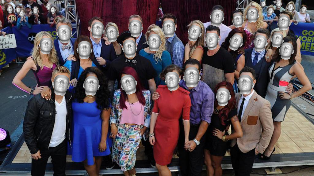
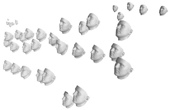
Figure 2: The 6DoF face poses estimated by our img2pose capture the positions of faces in the photo (top) and their 3D scene locations (bottom). See also Fig. 8 for a visualization of the 3D positions of all faces in WIDER FACE (val.).

A growing number of recent methods recognize that deep learning offers a way of directly regressing the face pose, in a landmark-free approach. Some directly estimated the 6DoF face pose from a face bounding box [8, 9, 10, 37, 52, 65, 82]. The impact of these landmark free alignment methods on downstream face recognition accuracy was evaluated and shown to improve results compared with landmark detection methods [9, 10]. HopeNet [65] extended these methods by training a network with multiple losses, showing significant performance improvement. FSA-Net [82] introduced a feature aggregation method to improve pose estimation. Finally, QuatNet [32] proposed a Quaternion-based face pose regression framework which claims to be more effective than Euler angle-based methods. All these methods rely on a face detection step, prior to pose estimation whereas our approach collapses these two to a single step.

Some of the methods listed above only regress 3DoF angular pose: the face yaw, pitch, and roll [65, 82] or rotational information [32]. For some use cases, this information suffices. Many other applications, however, including face alignment for recognition [28, 48, 49, 50, 75, 77], 3D reconstruction [21, 72, 73], face manipulation [55, 56, 57], also require the translational components of a full 6DoF pose. Our img2pose model, by comparison, provides full 6DoF face pose for every face in the photo (Fig. 2).

Finally, some noted that face alignment is often performed along with other tasks, such as face detection, landmark detection, and 3D reconstruction. They consequently proposed solving these problems together in a multi-task manner. Some early examples of this approach predate the recent rise of deep learning [58, 59]. More recent methods add face pose estimation or landmark detection heads to a face detection network [9, 38, 60, 61, 91]. It is unclear, however, if adding these tasks together improves or hurts the accuracy of the individual tasks. Indeed, evidence suggesting the latter is growing [46, 70, 89]. We leverage the observation that pose estimation already encapsulates face detection, thereby requiring only 6DoF pose as a single supervisory signal.

3 Proposed method

Given an image ${\bf I}$, we estimate 6DoF pose for each face, $i$ appearing in ${\bf I}$. We use ${{\bf{h}}_{i}}\in\mathbb{R}^{6}$ to denote each face pose:

$${{\bf{h}}_{i}}=(r_{x},r_{y},r_{z},t_{x},t_{y},t_{z}),$$ (1)

where $(r_{x},r_{y},r_{z})$ represent a rotation vector [71] and $(t_{x},t_{y},t_{z})$ is the 3D face translation.

It is well known that a 6DoF face pose, $\bf{h}$, can be converted to an extrinsic camera matrix for projecting a 3D face to the 2D image plane [23, 68]. Assuming known intrinsic camera parameters, the 3D face can then be aligned with a face in the photo [27, 28]. To our knowledge, however, previous work never leveraged this observation to propose replacing training for face bounding box detection with 6DoF pose estimation.

Specifically, assume a 3D face shape represented as a triangulated mesh. Points on the 3D face surface can be projected down to the photo using the standard pinhole model [26]:

$$[\mathbf{Q},\mathbf{1}]^{T}\sim\mathbf{K}[\mathbf{R},\mathbf{t}][\mathbf{P},\mathbf{1}]^{T},$$ (2)

where $\mathbf{K}$ is the intrinsic matrix (Sec. 3.2), $\mathbf{R}$ and $\mathbf{t}$ are the 3D rotation matrix and translation vector, respectively, obtained from $\bf{h}$ by standard means [23, 68], and $\mathbf{P}\in\mathbb{R}^{3\times n}$ is a matrix representing $n$ 3D points on the surface of the 3D face shape. Finally, $\mathbf{Q}\in\mathbb{R}^{2\times n}$ is the matrix representation of 2D points projected from 3D onto the image.

We use Eq. (2) to generate our qualitative figures, aligning the 3D face shape with each face in the photo (e.g., Fig. 1). Importantly, given the projected 2D points, $\mathbf{Q}$, a face detection bounding box can simply be obtained by taking the bounding box containing these 2D pixel coordinates.

It is worth noting that this approach provides better control over bounding box looseness and shapes, as shown in Fig. 3. Specifically, because the pose aligns a 3D shape with known geometry to a face region in the image, we can choose to modify face bounding boxes sizes and shapes to match our needs, e.g., including more of the forehead by expanding the box in the correct direction, invariant of pose.

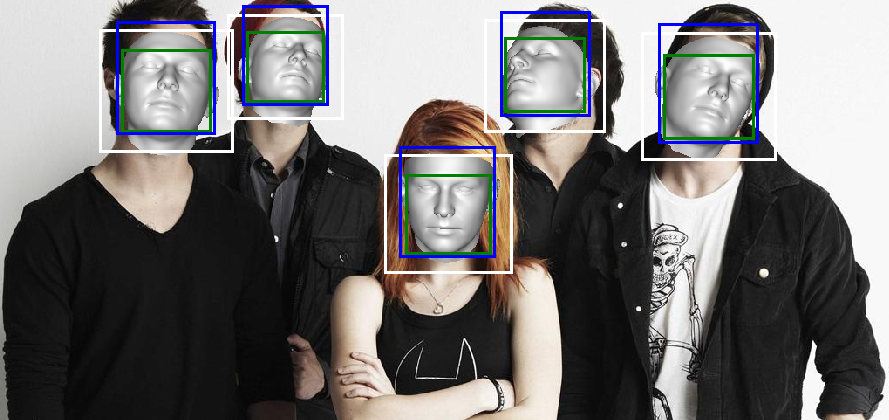
Figure 3: Bounding boxes generated using predicted poses. White bounding boxes generated with a loose setting, green with very tight setting, and blue with a less tight setting and forehead expansion (which is located through the pose).

3.1 Our img2pose network

We regress 6DoF face pose directly, based on the observation above that face bounding box information is already folded into the 6DoF face pose. Our network structure is illustrated in Fig. 4. Our network follows a two-stage approach based on Faster R-CNN [64]. The first stage is a region proposal network (RPN) with a feature pyramid [43], which proposes potential face locations in the image.

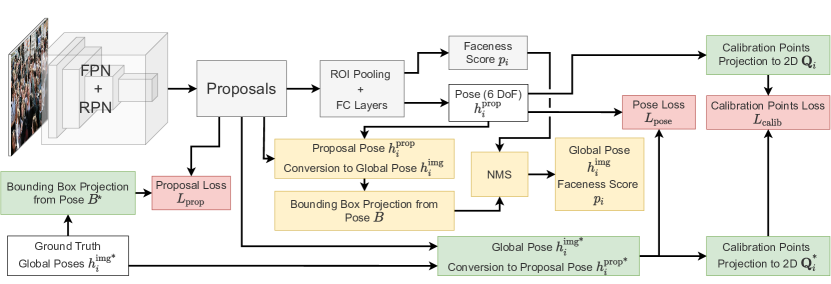
Figure 4: Overview of our proposed method. Components that only appear in training time are colored in green and red, and components that only appear in testing time are colored in yellow. Gray color denotes default components from Faster R-CNN with FPN [43, 64]. Please see Sec. 3 for more details.

Unlike the standard RPN loss, $L_{rpn}$, which uses ground-truth bounding box labels, we use projected bounding boxes, $\mathbf{B^{*}}$, obtained from the 6DoF ground-truth pose labels using Eq. (2) (see Fig. 4, $L_{prop}$). As explained above, by doing so, we gain better consistency in the facial regions covered by our bounding boxes, $\mathbf{B^{*}}$. Other aspects of this stage are similar to those of the standard Faster R-CNN [64], and we refer to their paper for technical details.

The second stage of our img2pose extracts features from each proposal with region of interest (ROI) pooling, and then passes them to two different heads: a standard face/non-face (faceness) classifier and a novel 6DoF face pose regressor (Sec. 3.3).

3.2 Pose label conversion

Two stage detectors rely on proposals – ad hoc image crops – as they train and while being evaluated. The pose regression head is provided with features extracted from proposals, not the entire image, and so does not have information required to determine where the face is located in the entire photo. This information is necessary because the 6DoF pose values are directly affected by image crop coordinates. For instance, a crop tightly matching the face would imply that the face is very close to the camera (small $t_{z}$ in Eq. (1)) but if the face appears much smaller in the original photo, this value would change to reflect the face being much farther away from the camera.

We therefore propose adjusting poses for different image crops, maintaining consistency between proposals and the entire photo. Specifically, for a given image crop we define a crop camera intrinsic matrix, $\mathbf{K}$, simply as:

$$\mathbf{K}=\begin{bmatrix}f&0&c_{x}\\ 0&f&c_{y}\\ 0&0&1\end{bmatrix}$$ (3)

Here, $f$ equals the face crop height plus width, and $c_{x}$ and $c_{y}$ are the $x,y$ coordinates of the crop center. Pose values are then converted between local (crop) and global (entire photo) coordinate frames, as follows.

Let matrix $\mathbf{K}_{img}$ be the projection matrix for the entire image, where $w$ and $h$ are the image width and height respectively, and $\mathbf{K}_{box}$ be the projection matrix for an arbitrary face crop (e.g., proposal), defined by $\mathbf{B}=(x,y,w_{bb},h_{bb})$, where $w_{bb}$ and $h_{bb}$ are the face crop width and height respectively, and $c_{x}$ and $c_{y}$ are the $x,y$ coordinates of the face crop’s center. We define these matrices as:

$$\mathbf{K}_{box}=\begin{bmatrix}w+h&0&c_{x}+x\\ 0&w+h&c_{y}+y\\ 0&0&1\end{bmatrix}$$ (4)

$$\mathbf{K}_{img}=\begin{bmatrix}w+h&0&w/2\\ 0&w+h&h/2\\ 0&0&1\end{bmatrix}$$ (5)

Converting pose from local to global frames. Given a pose, $\mathbf{h}^{prop}$, in a face crop coordinate frame, $\mathbf{B}$, intrinsic matrix, $\mathbf{K}_{img}$, for the entire image, intrinsic matrix, $\mathbf{K}_{box}$, for a face crop, we apply the method described in Algorithm 1 to convert $\mathbf{h}^{prop}$ to $\mathbf{h}^{img}$ (see Fig. 4).

Algorithm 1 Local to global pose conversion

1:procedure pose_convert($\mathbf{h}^{prop}$, $\mathbf{B}$, $\mathbf{K}_{box}$, $\mathbf{K}_{img}$)

2:     $f\leftarrow w+h$

3:     $t_{z}=t_{z}*f/(w_{bb}+h_{bb})$

4:     $\mathbf{V}=\mathbf{K}_{box}[t_{x},t_{y},t_{z}]^{T}$

5:     $[t^{\prime}_{x},t^{\prime}_{y},t^{\prime}_{z}]^{T}=(\mathbf{K}_{img})^{-1}\mathbf{V}$

6:     $\mathbf{R}=\text{rot\_vec\_to\_rot\_mat}([r_{x},r_{y},r_{z}])$

7:     $\mathbf{R^{\prime}}=(\mathbf{K}_{img})^{-1}\mathbf{K}_{box}\mathbf{R}$

8:     $(r^{\prime}_{x},r^{\prime}_{y},r^{\prime}_{z})=\text{rot\_mat\_to\_rot\_vec}(\mathbf{R^{\prime}})$

9:     return $\mathbf{h}^{img}=(r^{\prime}_{x},r^{\prime}_{y},r^{\prime}_{z},t^{\prime}_{x},t^{\prime}_{y},t^{\prime}_{z})$

Briefly, Algorithm 1 has two steps. First, in lines 2–3, we rescale the pose. Intuitively this step adjusts the camera to view the entire image, not just a crop. Then, in steps 4–8, we translate the focal point, adjusting the pose based on the difference of focal point locations, between the crop and the image. Finally, we return a 6DoF pose relative to the image intrinsic, $\mathbf{K}_{img}$. The functions rot_vec_to_rot_mat($\cdot$) and rot_mat_to_rot_vec($\cdot$) are standard conversion functions between rotation matrices and rotation vectors [26, 71]. Please see Appendix A for more details on this conversion.

Converting pose from global to local frames. To convert pose labels, $\mathbf{h}^{img}$, given in the image coordinate frame, to local crop frames, $\mathbf{h}^{prop}$, we apply a process similar to Algorithm 1. Here, $\mathbf{K}_{img}$ and $\mathbf{K}_{box}$ change roles, and scaling is applied last. We provide details of this process in Appendix A (see Fig. 4, $\mathbf{h}_{i}^{img*}$). This conversion is an important step, since, as previously mentioned, proposal crop coordinates vary constantly as the method is trained and so ground-truth pose labels given in the image coordinate frame must be converted to match these changes.

3.3 Training losses

We simultaneously train both the face/non-face classifier head and the face pose regressor. For each proposal, the model employs the following multi-task loss $L$.

$$\begin{split}L&=L_{cls}(p_{i},p^{*}_{i})+p^{*}_{i}\cdot L_{pose}(\mathbf{h}_{i}^{prop},\mathbf{h}_{i}^{prop*})\\ &+p^{*}_{i}\cdot L_{calib}(\mathbf{Q}^{c}_{i},\mathbf{Q}^{c*}_{i}),\end{split}$$ (6)

which includes these three components:

(1) Face classification loss. We use standard binary cross-entropy loss, $L_{cls}$, to classify each proposal, where $p_{i}$ is the probability of proposal $i$ containing a face and $p^{*}_{i}$ is the ground-truth binary label ($1$ for face and $0$ for background). These labels are determined by calculating the intersection over union (IoU) between each proposal and the ground-truth projected bounding boxes. For negative proposals which do not contain faces, ($p^{*}_{i}=0$), $L_{cls}$ is the only loss that we apply. For positive proposals, ($p^{*}_{i}=1$), we also evaluate the two novel loss functions described below.

(2) Face pose loss. This loss directly compares a 6DoF face pose estimate with its ground truth. Specifically, we define

$$L_{pose}(\mathbf{h}_{i}^{prop},\mathbf{h}_{i}^{prop*})=\left\lVert\mathbf{h}_{i}^{prop}-\mathbf{h}_{i}^{prop*}\right\rVert_{2}^{2},$$ (7)

where $\mathbf{h}_{i}^{prop}$ is the predicted face pose for proposal $i$ in the proposal coordinate frame, $\mathbf{h}_{i}^{prop*}$ is the ground-truth face pose in the same proposal (Fig. 4, $L_{pose}$). We follow the procedure mentioned in Sec. 3.2 to convert ground-truth poses, $\mathbf{h}_{i}^{img*}$, relative to the entire image, to ground-truth pose, $\mathbf{h}_{i}^{prop*}$, in a proposal frame.

(3) Calibration point loss. As an additional means of capturing the accuracy of estimated poses, we consider the 2D locations of projected 3D face shape points in the image (Fig. 4, $L_{calib}$). We compare points projected using the ground-truth pose vs. a predicted pose: An accurate pose estimate will project 3D points to the same 2D locations as the ground-truth pose (see Fig. 6 for a visualization). To this end, we select a fixed set of five calibration points, $\mathbf{P}^{c}\in\mathbb{R}^{5\times 3}$, on the surface of the 3D face. $\mathbf{P}^{c}$ is selected arbitrarily; we only require that they are not all co-planar.

Given a face pose, $\mathbf{h}\in\mathbb{R}^{6}$, either ground-truth or predicted, we can project $\mathbf{P}^{c}$ from 3D to 2D using Eq. (2). The calibration point loss is then defined as,

$$L_{calib}=\left\lVert\mathbf{Q}^{c}_{i}-\mathbf{Q}^{c*}_{i}\right\rVert_{1},$$ (8)

where $\mathbf{Q}_{i}^{c}$ are the calibration points projected from 3D using predicted pose $\mathbf{h}_{i}^{prop}$, and $\mathbf{Q}^{c*}_{i}$ is the calibration points projected using the ground-truth pose $\mathbf{h}_{i}^{prop*}$.

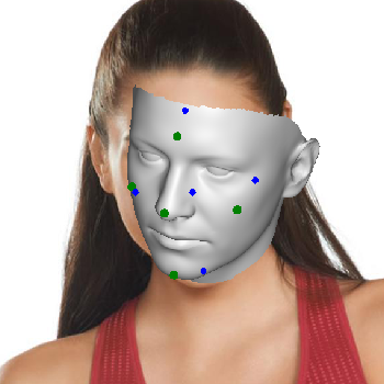
(a) Wrong Pose Estimation

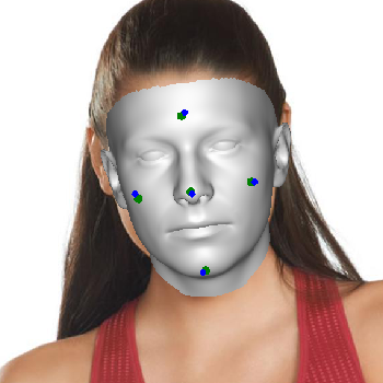
(b) Correct Pose Estimation

Figure 6: Visualizing our calibration points. (a) When the estimated pose is wrong, points projected from a 3D face to the photo (in green) fall far from the location of these same 3D point, projected using the ground truth (in blue); (b) With a better pose estimate, calibration points projected using the estimated pose fall closer to their locations following projection using the ground-truth pose.

4 Implementation details

4.1 Pose labeling for training and validation

We train our method on the WIDER FACE training set [81] (see also Sec. 5.4). WIDER FACE offers manually annotated bounding box labels, but no labels for pose. The RetinaFace project [18], however, provides manually annotated, five point facial landmarks for 76k of the WIDER FACE training faces. We increase the number of training pose labels as well as provide pose annotations for the validation set, using the following weakly supervised manner.

We run the RetinaFace face bounding box and five point landmark detector on all images containing face box annotations but missing landmarks. We take RetinaFace predicted bounding boxes which have the highest IoU ratio with the ground-truth face box label, unless their IoU is smaller than $0.5$. We then use the box predicted by RetinaFace along with its five landmarks to obtain 6DoF pose labels for these faces, using standard means [17, 40]. Importantly, neither box or landmarks are then stored or used in our training; only the 6DoF estimates are kept. Finally, poses are converted to their global, image frames using the process described in Sec. 3.2.

This process provided us with $12,874$ images containing $138,722$ annotated training faces of which $62,827$ were assigned with weakly supervised poses. Our validation set included $3,205$ images with $34,294$ pose annotated faces, all of which were weakly supervised. During training, we ignore faces which do not have pose labels.

Data augmentation. Similar to others [84], we process our training data, augmenting it to improve the robustness of our method. Specifically, we apply random crop, mirroring and scale transformations to the training images. Multiple scales were produced for each training image, where we define the minimum size of an image as either $640$, $672$, $704$, $736$, $768$, $800$, and the maximum size is set as $1400$.

4.2 Training details

We implemented our img2pose approach in PyTorch using ResNet-$18$ [29] as backbone. We use stochastic gradient descent (SGD) with a mini batch of two images. During training, $256$ proposals per image are sampled for the RPN loss computation and $512$ samples per image for the pose head losses. Learning rate starts at $0.001$ and is reduced by a factor of $10$ if the validation loss does not improve over three epochs. Early stop is triggered if the model does not improve for five consecutive epochs on the validation set. Finally, the main training took $35$ epochs. On a single NVIDIA Quadro RTX $6000$ machine, training time was roughly $4$ days.

For face pose evaluation, Euler angles are the standard metric in the benchmarks used. Euler angles suffer from several drawbacks [7, 32], when dealing with large yaw angles. Specifically, when yaw angle exceeds $\pm 90^{\circ}$, any small change in yaw will cause significant differences in pitch and roll (See [7] Sec. 4.5 for an example of this issue). Given that the WIDER FACE dataset contains many faces whose yaw angles are larger than $\pm 90^{\circ}$, to overcome this issue, for face pose evaluation, we fine-tuned our model on 300W-LP [90], which only contains face poses with yaw angles in the range of $(-90,+90)$.

300W-LP is a dataset with synthesized head poses from 300W [66] containing $122,450$ images. Training pose rotation labels are obtained by converting the 300W-LP ground-truth Euler angles to rotation vectors, and pose translation labels are created using the ground-truth landmarks, using standard means [17, 40]. During fine-tuning, $2$ proposals per image are sampled for the RPN loss and $4$ samples per image for the pose head losses. Finally, learning rate is kept fixed at $0.001$ and the model is fine-tuned for $2$ epochs.

Method	Direct?	Yaw	Pitch	Roll	MAEr	X	Y	Z	MAEt
Dlib (68 points) [34]	✗	18.273	12.604	8.998	13.292	0.122	0.088	1.130	0.446
3DDFA [90] $\dagger$	✗	5.400	8.530	8.250	7.393	-	-	-	-
FAN (12 points) [4] $\dagger$	✗	6.358	12.277	8.714	9.116	-	-	-	-
Hopenet ($\alpha=2$) [65] $\dagger$	✗	6.470	6.560	5.440	6.160	-	-	-	-
QuatNet [32] $\dagger$	✗	3.973	5.615	3.920	4.503	-	-	-	-
FSA-Caps-Fusion [82]	✗	4.501	6.078	4.644	5.074	-	-	-	-
HPE [33] $\dagger$	✗	4.870	6.180	4.800	5.280	-	-	-	-
TriNet [7] $\dagger$	✗	4.198	5.767	4.042	4.669	-	-	-	-
RetinaFace R-50 (5 points) [18]	✓	5.101	9.642	3.924	6.222	0.038	0.049	0.255	0.114
img2pose (ours)	✓	3.426	5.034	3.278	3.913	0.028	0.038	0.238	0.099

Table 1: Pose estimation accuracy on AFLW2000-3D [90]. $\dagger$ denotes results reported by others. Direct methods, like ours, were not tested on the ground-truth face crops, which capture scale information. Some methods do not produce or did not report translational accuracy. Finally, MAE_r and MAE_t are the Euler angles and translational MAE, respectively. On a $400\times 400$ pixel image from AFLW2000, our method runs at 41 fps.

Method	Direct?	Yaw	Pitch	Roll	MAEr
Dlib (68 points) [34] $\dagger$	✗	16.756	13.802	6.190	12.249
3DDFA [90] $\dagger$	✗	36.175	12.252	8.776	19.068
FAN (12 points) [4] $\dagger$	✗	8.532	7.483	7.631	7.882
Hopenet ($\alpha=1$) [65] $\dagger$	✗	4.810	6.606	3.269	4.895
QuatNet [32] $\dagger$	✗	4.010	5.492	2.936	4.146
FSA-NET [82] $\dagger$	✗	4.560	5.210	3.070	4.280
HPE [33] $\dagger$	✗	4.570	5.180	3.120	4.290
TriNet [7] $\dagger$	✗	3.046	4.758	4.112	3.972
RetinaFace R-50 (5 pnt.) [18]	✓	4.070	6.424	2.974	4.490
img2pose (ours)	✓	4.567	3.546	3.244	3.786

Table 2: Comparison of the state-of-the-art methods on the BIWI dataset. Methods marked with $\dagger$ are reported by others. Direct methods, like ours, were not tested on ground truth face crops, which capture scale information. On $933\times 700$ BIWI images, our method runs at 30 fps.

5 Experimental results

5.1 Face pose tests on AFLW2000-3D

AFLW2000-3D [90] contains the first $2$k faces of the AFLW dataset [35] along with ground-truth 3D faces and corresponding $68$ landmarks. The images in this set have a large variation of pose, illumination, and facial expression. To create ground-truth translation pose labels for AFLW2000-3D, we follow the process described in Sec. 4.1. We convert the manually annotated 68-point, ground-truth landmarks, available as part of AFLW2000-3D, to 6DoF pose labels, keeping only the translation part. For the rotation part, we use the provided ground-truth in Euler angles (pitch, yaw, roll) format, where the predicted rotation vectors are converted to Euler angles for comparison. We follow others [65, 82] by removing images with head poses that are not in the range of $[-99,+99]$, discarding only $31$ out of the $2,000$ images.

We test our method and its baselines on each image, scaled to $400\times 400$ pixels. Because some AFLW2000-3D images show multiple faces, we select the face that has the highest IoU between bounding boxes projected from predicted face poses and ground-truth bounding boxes, which were obtained by expanding the ground-truth landmarks. We verified the set of faces selected in this manner and it is identical to the faces marked by the ground-truth labels.

AFLW2000-3D face pose results. Table 1 compares our pose estimation accuracy with SotA methods on AFLW2000-3D. Importantly, aside from RetinaFace [18], all other methods are applied to manually cropped face boxes and not directly to the entire photo. Ground truth boxes provide these methods with 2D face translation and, importantly, scale for either pose of landmarks. This information is unavailable to our img2pose which takes the entire photo as input. Remarkably, despite having less information than its baselines, our img2pose reports a SotA MAE_r of 3.913, while running at 41 frames per second (fps) with a single Titan Xp GPU.

Other than our img2pose, the only method that processes input photos directly is RetinaFace [18]. Our method outperforms it, despite the much larger, ResNet-50 backbone used by RetinaFace, its greater supervision in using not only bounding boxes and five point landmarks, but also per-subject 3D face shapes, and its more computationally demanding training. This result is even more significant, considering that this RetinaFace model was used to generate some of our training labels (Sec. 4.1). We believe our superior results are due to img2pose being trained to solve a simpler, 6DoF pose estimation problem, compared with the RetinaFace goal of bounding box and landmark regression.

5.2 Face pose tests on BIWI

BIWI [20] contains $15,678$ frames of $20$ subjects in an indoor environment, with a wide range of face poses. This benchmark provides ground-truth labels for rotation (rotation matrix), but not for the translational elements required for full 6DoF. Similar to AFLW2000-3D, we convert the ground-truth rotation matrix and prediction rotation vectors to Euler angles for comparison. We test our method and its baselines on each image using $933\times 700$ pixels resolution. Because many images in BIWI contain more than a single face, to compare our predictions, we selected the face that is closer to the center of the image with a face score $p_{i}>0.9$. Here, again, we verified that our direct method detected and processed all the faces supplied with test labels.

BIWI face pose results. Table 2 reports BIWI results following protocol 1 [65, 82] where models are trained with external data and tested in the entire BIWI dataset. Similarly to the results on AFLW2000, Sec. 5.1, our pose estimation results again outperform the existing SotA, despite being applied to the entire image, without pre-cropped and scaled faces, reporting MAE_r of 3.786. Finally, img2pose runtimeon the original $933\times 700$ BIWI images is 30 fps.

			Validation			Test
Method	Backbone	Pose?	Easy	Med.	Hard	Easy	Med.	Hard
SotA methods using heavy backbones (provided for completeness)
SRN [11]	R-50	✗	0.964	0.953	0.902	0.959	0.949	0.897
DSFD [42]	R-50	✗	0.966	0.957	0.904	0.960	0.953	0.900
PyramidBox++ [69]	R-50	✗	0.965	0.959	0.912	0.956	0.952	0.909
RetinaFace [18]	R-152	✓*	0.971	0.962	0.920	0.965	0.958	0.914
ASFD-D6 [83]	-	✗	0.972	0.965	0.925	0.967	0.962	0.921
Fast / small backbone face detectors
Faceboxes [86]	-	✗	0.879	0.857	0.771	0.881	0.853	0.774
FastFace [85]	-	✗	-	-	-	0.833	0.796	0.603
LFFD [30]	-	✗	0.910	0.881	0.780	0.896	0.865	0.770
RetinaFace-M [18]	MobileNet	✓*	0.907	0.882	0.738	-	-	-
ASFD-D0 [83]	-	✗	0.901	0.875	0.744	-	-	-
Luo et al.[47]	-	✗	-	-	-	0.902	0.878	0.528
img2pose (ours)	R-18	✓	0.908	0.899	0.847	0.900	0.891	0.839

Figure 7: WIDER FACE results. ’*’ Requires PnP to get pose from landmarks. Our img2pose surpasses other light backbone detectors on Med. and Hard sets, despite not being trained to detect faces.

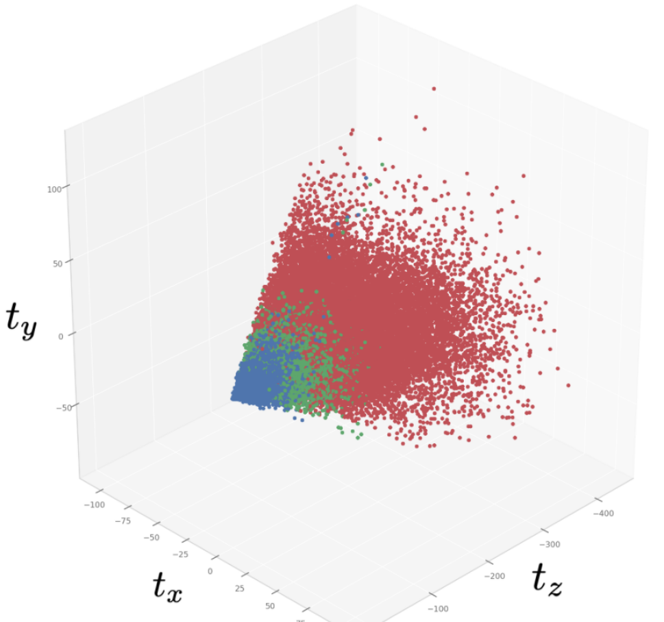
Figure 8: Visualizing our estimated pose translations on WIDER FACE val. images. Colors encode Easy (blue), Med. (green), and Hard (red). Easy faces seem centered close to the camera whereas Hard faces are far more distributed in the scene.

5.3 Ablation study

We examine the effect of our loss functions, defined in Sec. 3.3, where we compare our results following training with only the face pose loss, $L_{pose}$, only the calibration points loss, $L_{calib}$, and both loss functions combined.

Table 3 provides our ablation results. The table compares the three loss variations using $MAE_{r}$ and $MAE_{t}$ on the AFLW2000-3D set and $MAE_{r}$ on BIWI. Evidently, combining both loss functions leads to improved accuracy in estimating head rotations, with the gap on BIWI being particularly wide, in favor of the combined loss. Curiously, translation errors on AFLW2000-3D are somewhat higher with the joint loss compared to the use of either loss function, individually. Still, these differences are small and could be attributed to stochasticity in the model training due to random initialization and random augmentations applied during training (see Sec. 4.1 and 4.2).

Loss	AFLW2000-3D		BIWI
	MAEr	MAEt	MAEr
$L_{pose}$	5.305	0.114	4.375
$L_{calib}$	4.746	0.118	4.023
$L_{pose}$ + $L_{calib}$	4.657	0.125	3.856

Table 3: Comparison of the effects of different loss functions on the pose estimation results obtained on the AFLW2000-3D and BIWI benchmarks. MAE_r and MAE_t are the rotational and translational MAE, respectively.

5.4 Face detection on WIDER FACE

Our method outperforms SotA methods for face pose estimation on two leading benchmarks. Because it is applied to the input images directly, it is important to verify how accurate is it in detecting faces. To this end, we evaluate our img2pose on the WIDER FACE benchmark [81]. WIDER FACE offers $32,203$ images with $393,703$ faces annotated with bounding box labels. These images are partitioned into $12,880$ training, $3,993$ validation, and $16,097$ testing images, respectively. Results are reported in terms of detection mean average precision (mAP), on the WIDER FACE easy, medium, and hard subsets, for both validation and test sets.

We train our img2pose on the WIDER FACE training set and evaluate on the validation and test sets using standard protocols [18, 54, 88], including application of flipping, and multi-scaling testing, with the shorter sides of the image scaled to $[500,800,1100,1400,1700]$ pixels. We use the process described in Sec. 3 to project points from a 3D face shape onto the image and take a bounding box containing the projected points as a detected bounding box (See also Fig. 4). Finally, box voting [24] is applied on the projected boxes, generated at different scales.

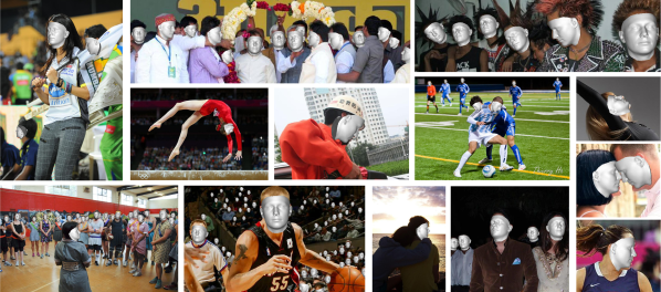
Figure 9: Qualitative img2pose results on WIDER FACE validation images [81]. In all cases, we only estimate 6DoF face poses, directly from the photo, and without a preliminary face detection step. For more samples, please see Appendix B for more results.

WIDER FACE detection results. Table 8 compares our results to existing methods. Importantly, the design of our img2pose is motivated by run-time. Hence, with a ResNet-18 backbone, it cannot directly compete with far heavier, SotA face detectors. Although we provide a few SotA results for completeness, we compare our results with methods that, similarly to us, use light and efficient backbones.

Evidently, our img2pose outperforms models of comparable complexity in the validation and test, Medium and Hard partitions. This results is remarkable, considering that our method is the only one that provides 6DoF pose and direct face alignment, and not only detects faces. Moreover, our method is trained with 20k less faces than prior work. We note that RetinaFace [18] returns five face landmarks which can, with additional processing, be converted to 6DoF pose. Our img2pose, however, reports better face detection accuracy than their light model and substantially better pose estimation as evident from Sec. 5.1 and Sec. 5.2.

Fig. 8 visualizes the 3D translational components of our estimated 6DoF poses, for WIDER FACE validation images. Each $(t_{x},t_{y},t_{z})$ point is color coded by: Easy (blue), Medium (green), and Hard (red). This figure clearly shows how faces in the easy set congregate close to the camera and in the center of the scene, whereas faces from the Medium and Hard sets vary more in their scene locations, with Hard especially scattered, which explains the challenge of that set and testifies to the correctness of our pose estimates.

Fig. 9 provides qualitative samples of our img2pose on WIDER FACE validation images. We observe that our method can generate accurate pose estimation for faces with various pitch, yaw, roll angles, and for images under various scale, illumination, occlusion variations. These results demonstrate the effectiveness of img2pose for direct pose estimation and face detection.

6 Conclusions

We propose a novel approach to 6DoF face pose estimation and alignment, which does not rely on first running a face detector or localizing facial landmarks. To our knowledge, we are the first to propose such a multi-face, direct approach. We formulate a novel pose conversion algorithm to maintain consistency of poses estimated for the same face across different image crops. We show that face bounding box can be generated via the estimated 3D face pose – achieving face detection as a byproduct of pose estimation. Extensive experiments have demonstrated the effectiveness of our img2pose for face pose estimation and face detection.

As a class, faces offer excellent opportunities to this marriage of pose and detection: faces have well-defined appearance statistics which can be relied upon for accurate pose estimation. Faces, however, are not the only category where such an approach may be applied; the same improved accuracy may be obtained in other domains, e.g., retail [25], by applying a similar direct pose estimation step as a substitute for object and key-point detection.

Appendix A Pose conversion methods

We elaborate on our pose conversion algorithms, mentioned in Sec. 3.2. Algorithm 1 starts with an initial pose $\mathbf{h}^{prop}$ estimated relative to an image crop, $B$ (see, Fig. 10(b)), and produces the final converted pose, $\mathbf{h}^{img}$, relative to the whole image, $I$ (in Fig. 10(d)).

At a high level, our pose conversion algorithm, Algorithm 1, consists of the following two steps:

The first step is a rescaling step (from Fig. 10(b) to Fig. 10(c)), where we adjust the camera to view the entire image, $I$, not just the crop, $B$. After the first step, we obtain an intermediate pose representation, $\mathbf{h}^{intermediate}$, relative to the camera location, assumed in Fig. 10(c).

The second step is a translation step (from Fig.. 10(c) to Fig. 10(d)), where we translate the principal / focal point of the camera from the center of the crop region to image center. After this step, each converted global pose, $\mathbf{h}^{img}$, from different crop, $B_{i}$, is estimated based on a consistent camera location, as shown in Fig. 10(d).

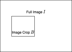
(a) An example photo

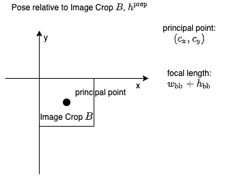
(b) Initial pose estimation $h^{prop}$

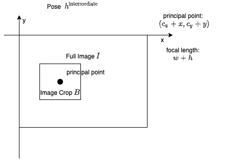
(c) Intermediate pose estimation $h^{intermediate}$ (Line 2 - 3)

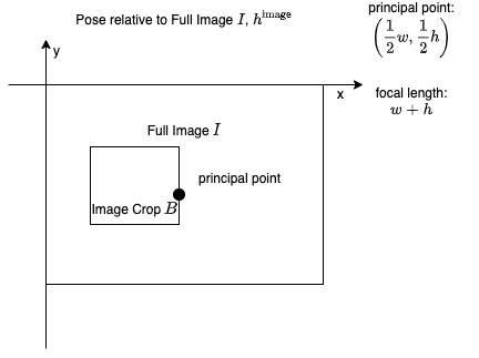
(d) Final pose estimation $h^{image}$ (Line 4 - 8)

Figure 10: Illustrating the pose conversion method. See Sec. A for more details.

Each pose, $\mathbf{h}^{prop}$, $\mathbf{h}^{intermediate}$, and $\mathbf{h}^{image}$, is associated with a specific assumed camera location and thus a specific intrinsic camera matrix, $\mathbf{K}$, $\mathbf{K}_{box}$, and $\mathbf{K}_{img}$ respectively, where we define again here.

Here, we assume $f$ equals the image crop height, $h_{bb}$, plus width, $w_{bb}$, $c_{x}$ and $c_{y}$ are the $x,y$ coordinates of the image crop center, respectively, and $w$, $h$ are the full image width and height respectively.

$$\mathbf{K}=\begin{bmatrix}f&0&c_{x}\\ 0&f&c_{y}\\ 0&0&1\end{bmatrix},$$ (9)

$$\mathbf{K}_{box}=\begin{bmatrix}w+h&0&c_{x}+x\\ 0&w+h&c_{y}+y\\ 0&0&1\end{bmatrix},$$ (10)

$$\mathbf{K}_{img}=\begin{bmatrix}w+h&0&w/2\\ 0&w+h&h/2\\ 0&0&1\end{bmatrix}.$$ (11)

The input to Algorithm 1 $\mathbf{h}^{prop}$ is estimated based on camera matrix, $\mathbf{K}$, whose principal point is at the center of the image crop $B$, $(c_{x},c_{y})$, and focal length $f$ is $w_{bb}+h_{bb}$, which is visualized in Fig. 10(b). Step 1 of the algorithm, lines 2-3, first rescales the image. This zoom-out operation pushes the object further away from the camera by multiplying the translation on the $z$ axis, $t_{z}$, with the factor $(w+h)/(w_{bb}+h_{bb})$. This extra factor in $z$ will adjust the projected coordinates, $p$, on the image plane to reflect the relative ratio of the image crop to the whole image (since the original pose estimate $\mathbf{h}^{prop}$ is estimated assuming each image crop is of constant size).

Then we also adjust, accordingly, the camera matrices from $\mathbf{K}$ to $\mathbf{K}_{box}$. This transformation in intrinsic camera matrices will adjust the principal point, and thus the origin of the image coordinates system from the top left corner of the image crop to the top left corner of the whole image.

Step 2 of the algorithm, lines 4-8, translates the camera, so that every pose estimate, $\mathbf{h}^{img}$, is based on the camera settings shown in Fig. 10(d) with principal point at image center and focal length $w+h$.

The methodology here is to first adjust the camera matrix from $\mathbf{K}_{box}$ to $\mathbf{K}_{img}$, in order to compensate the translation of our desired principal points, and then solve for the associated pose, $\mathbf{h}^{img}$. Since the image coordinate system does not change in Step 2, the following equality must hold,

$$\mathbf{p}=\mathbf{K}_{box}[\mathbf{R}|\mathbf{t}]\mathbf{P},$$

$$\mathbf{p}=\mathbf{K}_{img}[\mathbf{R^{\prime}}|\mathbf{t^{\prime}}]\mathbf{P}.$$

In other words,

$$\mathbf{K}_{box}[\mathbf{R}|\mathbf{t}]=\mathbf{K}_{img}[\mathbf{R^{\prime}}|\mathbf{t^{\prime}}].$$

So we can obtain the rotation matrices $\mathbf{R^{\prime}}$ and translation vectors $\mathbf{t}^{\prime}$ by the following equations,

$$\mathbf{R^{\prime}}=(\mathbf{K}_{img})^{-1}\mathbf{K}_{box}\mathbf{R},$$

$$\mathbf{t^{\prime}}=(\mathbf{K}_{img})^{-1}\mathbf{K}_{box}\mathbf{t}.$$

The new pose, $\mathbf{h}^{img}$, can then be extracted from $\mathbf{R^{\prime}}$ and $\mathbf{t}^{\prime}$ using standard approaches [14, 26]

The conversion from global pose, $\mathbf{h}^{img}$, to local pose, $\mathbf{h}^{prop}$, follows the exact same methodology. For completeness, we provide pseudo-code for this step in Algorithm 2.

Algorithm 2 Global to local pose conversion

1:procedure pose_convert($\mathbf{h}^{img}$, $\mathbf{B}$, $\mathbf{K}_{box}$, $\mathbf{K}_{img}$)

2:     $\mathbf{V}=\mathbf{K}_{img}[t_{x},t_{y},t_{z}]^{T}$

3:     $[t^{\prime}_{x},t^{\prime}_{y},t^{\prime}_{z}]^{T}=(\mathbf{K}_{box})^{-1}\mathbf{V}$

4:     $\mathbf{R}=\text{rot\_vec\_to\_rot\_mat}([r_{x},r_{y},r_{z}])$

5:     $\mathbf{R^{\prime}}=(\mathbf{K}_{box})^{-1}\mathbf{K}_{img}\mathbf{R}$

6:     $(r^{\prime}_{x},r^{\prime}_{y},r^{\prime}_{z})=\text{rot\_mat\_to\_rot\_vec}(\mathbf{R^{\prime}})$

7:     $f\leftarrow w+h$

8:     $t^{\prime}_{z}=t^{\prime}_{z}/f*(w_{bb}+h_{bb})$

9:     return $\mathbf{h}^{prop}=(r^{\prime}_{x},r^{\prime}_{y},r^{\prime}_{z},t^{\prime}_{x},t^{\prime}_{y},t^{\prime}_{z})$

Appendix B Qualitative results

We provide an abundance of qualitative results in Fig. 11,  12 and 13. Fig. 11 visually compares the pose estimated by our img2pose with the ground-truth pose labels on the AFLW2000-3D set images [90]. Our method is clearly robust to a wide range of face poses, as also evident from its state of the art (SotA) numbers reported in Table 1. The last row in Fig. 11 offers samples where our method did not accurately predict the correct pose.

Fig. 12 offers qualitative results on BIWI images [20], comparing our estimated poses with ground truth labels. BIWI provides ground truth angular and translational pose labels. Because we do not have information on the world (3D) coordinates used by BIWI to define their translations, we could only use their rotational ground truth values. The visual comparison should therefore only focus on the angular components of the pose.

Our img2pose evidently predicts accurate poses, consistent with the quantitative results reported in Table 2. It is worth noting that BIWI faces are often smaller in size, relative to the entire photos, compared to the face to image sizes in AFLW2000-3D. Nevertheless, our direct method successfully predicts accurate poses. The last row of Fig. 12 provides sample pose errors.

Finally, Fig. 13 provides qualitative results on the WIDER FACE validation set images [81]. The images displayed show the robustness of our method across a wide range of scenarios, with varying illumination, scale, large face poses and occlusion.

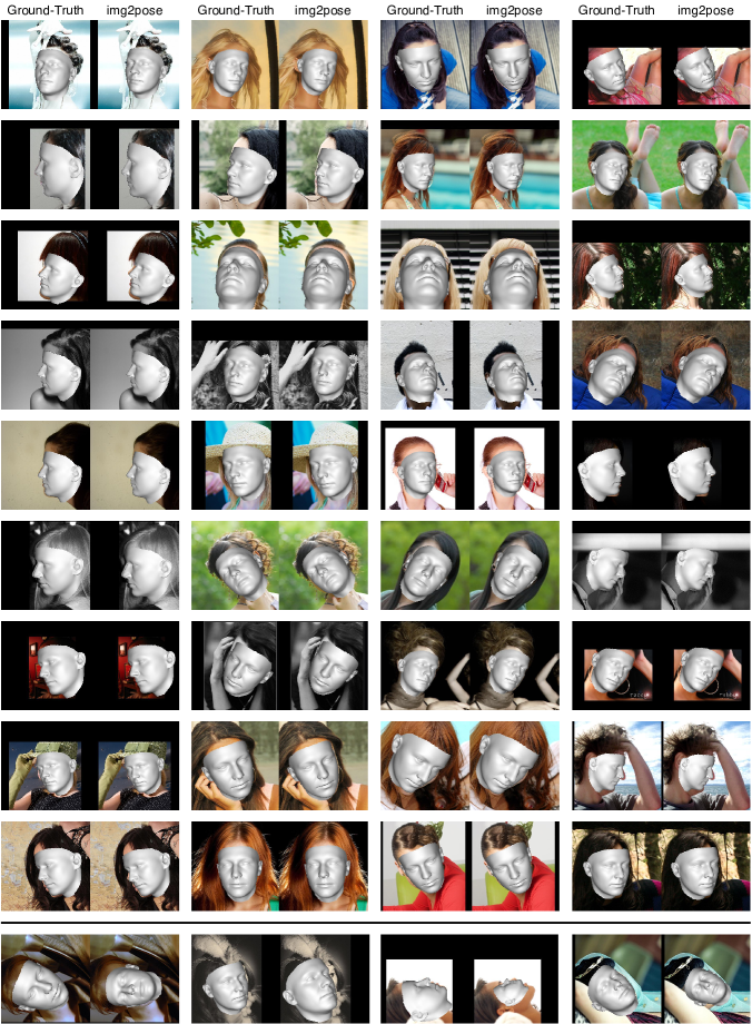
Figure 11: Qualitative comparing the results of our img2pose method on images from the AFLW2000-3D set to the ground truth poses. Poses visualized using a 3D face shape rendered using the pose on input photos. We provide results reflecting a wide range of face poses and viewing settings. The bottom row provides sample qualitative errors.

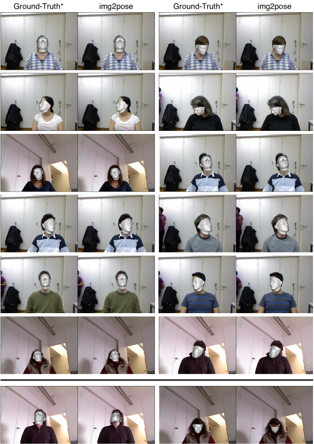
Figure 12: Qualitative pose estimation results on BIWI images, comparing the poses estimated by our img2pose with the ground truth. These results demonstrate how well our method correctly estimates poses for even small faces. The bottom row provides samples of the limitations of our model. Note that in all these images, the translation component of the pose, $(t_{x},t_{y},t_{z})$, was estimated by our img2pose both for our results and the ground truth, as ground truth labels do not provide this information.

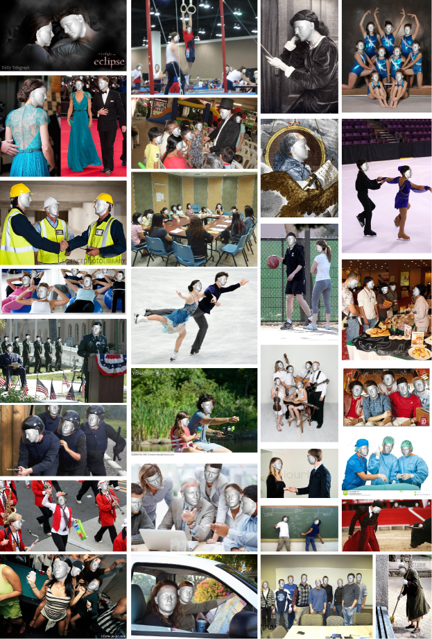
Figure 13: Qualitative face detection results of our img2pose method on photos from the WIDER FACE validation set. Note that despite not being directly trained to detect faces, our method captures even the smallest faces appearing in the background as well as estimates their poses (zoom in for better views).

References

- [1] Vítor Albiero and Kevin W. Bowyer. Is face recognition sexist? no, gendered hairstyles and biology are. In Proc. British Mach. Vision Conf., 2020.
- [2] Vítor Albiero, Kai Zhang, and Kevin W. Bowyer. How does gender balance in training data affect face recognition accuracy? In Winter Conf. on App. of Comput. Vision, 2020.
- [3] Bjorn Browatzki and Christian Wallraven. 3FabRec: Fast few-shot face alignment by reconstruction. In Proc. Conf. Comput. Vision Pattern Recognition, pages 6110–6120, 2020.
- [4] Adrian Bulat and Georgios Tzimiropoulos. How far are we from solving the 2d & 3d face alignment problem? (and a dataset of 230,000 3d facial landmarks). In Proc. Int. Conf. Comput. Vision, pages 1021–1030, 2017.
- [5] Xavier P Burgos-Artizzu, Pietro Perona, and Piotr Dollár. Robust face landmark estimation under occlusion. In Proc. Int. Conf. Comput. Vision, pages 1513–1520, 2013.
- [6] Xudong Cao, Yichen Wei, Fang Wen, and Jian Sun. Face alignment by explicit shape regression. Int. J. Comput. Vision, 107(2):177–190, 2014.
- [7] Zhiwen Cao, Zongcheng Chu, Dongfang Liu, and Yingjie Chen. A vector-based representation to enhance head pose estimation. arXiv preprint arXiv:2010.07184, 2020.
- [8] Feng-Ju Chang, Anh Tuan Tran, Tal Hassner, Iacopo Masi, Ram Nevatia, and Gerard Medioni. ExpNet: Landmark-free, deep, 3D facial expressions. In Int. Conf. on Automatic Face and Gesture Recognition, pages 122–129. IEEE, 2018.
- [9] Feng-Ju Chang, Anh Tuan Tran, Tal Hassner, Iacopo Masi, Ram Nevatia, and Gérard Medioni. Deep, landmark-free FAME: Face alignment, modeling, and expression estimation. Int. J. Comput. Vision, 127(6-7):930–956, 2019.
- [10] Feng-Ju Chang, Anh Tuan Tran, Tal Hassner, Iacopo Masi, Ram Nevatia, and Gerard Medioni. FacePoseNet: Making a case for landmark-free face alignment. In Proc. Int. Conf. Comput. Vision Workshops, pages 1599–1608, 2017.
- [11] Cheng Chi, Shifeng Zhang, Junliang Xing, Zhen Lei, Stan Z Li, and Xudong Zou. Selective refinement network for high performance face detection. In Conf. of Assoc for the Advanc. of Artificial Intelligence, volume 33, pages 8231–8238, 2019.
- [12] Timothy F Cootes, Gareth J Edwards, and Christopher J Taylor. Active appearance models. In European Conf. Comput. Vision, pages 484–498. Springer, 1998.
- [13] Jifeng Dai, Yi Li, Kaiming He, and Jian Sun. R-fcn: Object detection via region-based fully convolutional networks. In Neural Inform. Process. Syst., pages 379–387, 2016.
- [14] Jian S Dai. Euler–rodrigues formula variations, quaternion conjugation and intrinsic connections. Mechanism and Machine Theory, 92:144–152, 2015.
- [15] Navneet Dalal and Bill Triggs. Histograms of oriented gradients for human detection. In Proc. Conf. Comput. Vision Pattern Recognition, volume 1, pages 886–893. IEEE, 2005.
- [16] Arnaud Dapogny, Kevin Bailly, and Matthieu Cord. DeCaFA: deep convolutional cascade for face alignment in the wild. In Proc. Int. Conf. Comput. Vision, pages 6893–6901, 2019.
- [17] Daniel F Dementhon and Larry S Davis. Model-based object pose in 25 lines of code. Int. J. Comput. Vision, 15(1-2):123–141, 1995.
- [18] Jiankang Deng, Jia Guo, Evangelos Ververas, Irene Kotsia, and Stefanos Zafeiriou. Retinaface: Single-shot multi-level face localisation in the wild. In Proc. Conf. Comput. Vision Pattern Recognition, pages 5203–5212, 2020.
- [19] Jiankang Deng, Jia Guo, Niannan Xue, and Stefanos Zafeiriou. Arcface: Additive angular margin loss for deep face recognition. In Proc. Conf. Comput. Vision Pattern Recognition, pages 4690–4699, 2019.
- [20] Gabriele Fanelli, Matthias Dantone, Juergen Gall, Andrea Fossati, and Luc Van Gool. Random forests for real time 3d face analysis. Int. J. Comput. Vision, 101(3):437–458, 2013.
- [21] Yao Feng, Fan Wu, Xiaohu Shao, Yanfeng Wang, and Xi Zhou. Joint 3d face reconstruction and dense alignment with position map regression network. In European Conf. Comput. Vision, pages 534–551, 2018.
- [22] Zhen-Hua Feng, Josef Kittler, Muhammad Awais, Patrik Huber, and Xiao-Jun Wu. Face detection, bounding box aggregation and pose estimation for robust facial landmark localisation in the wild. In Proc. Conf. Comput. Vision Pattern Recognition Workshops, pages 160–169, 2017.
- [23] David A Forsyth and Jean Ponce. Computer vision: a modern approach. Prentice Hall Professional Technical Reference, 2002.
- [24] Spyros Gidaris and Nikos Komodakis. Object detection via a multi-region and semantic segmentation-aware CNN model. In Proc. Int. Conf. Comput. Vision, pages 1134–1142, 2015.
- [25] Eran Goldman, Roei Herzig, Aviv Eisenschtat, Jacob Goldberger, and Tal Hassner. Precise detection in densely packed scenes. In Proc. Conf. Comput. Vision Pattern Recognition, pages 5227–5236, 2019.
- [26] Richard Hartley and Andrew Zisserman. Multiple view geometry in computer vision. Cambridge university press, 2003.
- [27] Tal Hassner. Viewing real-world faces in 3d. In Proc. Int. Conf. Comput. Vision, pages 3607–3614, 2013.
- [28] Tal Hassner, Shai Harel, Eran Paz, and Roee Enbar. Effective face frontalization in unconstrained images. In Proc. Conf. Comput. Vision Pattern Recognition, pages 4295–4304, 2015.
- [29] Kaiming He, Xiangyu Zhang, Shaoqing Ren, and Jian Sun. Deep residual learning for image recognition. In CVPR, pages 770–778, 2016.
- [30] Yonghao He, Dezhong Xu, Lifang Wu, Meng Jian, Shiming Xiang, and Chunhong Pan. Lffd: A light and fast face detector for edge devices. arXiv preprint arXiv:1904.10633, 2019.
- [31] Matthias Hernandez, Tal Hassner, Jongmoo Choi, and Gerard Medioni. Accurate 3d face reconstruction via prior constrained structure from motion. Computers & Graphics, 66:14–22, 2017.
- [32] Heng-Wei Hsu, Tung-Yu Wu, Sheng Wan, Wing Hung Wong, and Chen-Yi Lee. Quatnet: Quaternion-based head pose estimation with multiregression loss. IEEE Transactions on Multimedia, 21(4):1035–1046, 2018.
- [33] Bin Huang, Renwen Chen, Wang Xu, and Qinbang Zhou. Improving head pose estimation using two-stage ensembles with top-k regression. Image and Vision Computing, 93:103827, 2020.
- [34] Vahid Kazemi and Josephine Sullivan. One millisecond face alignment with an ensemble of regression trees. In Proc. Conf. Comput. Vision Pattern Recognition, pages 1867–1874, 2014.
- [35] Martin Koestinger, Paul Wohlhart, Peter M Roth, and Horst Bischof. Annotated facial landmarks in the wild: A large-scale, real-world database for facial landmark localization. In Proc. Int. Conf. Comput. Vision Workshops, pages 2144–2151. IEEE, 2011.
- [36] K. S. Krishnapriya, Vítor Albiero, Kushal Vangara, Michael C. King, and Kevin W. Bowyer. Issues related to face recognition accuracy varying based on race and skin tone. Trans. Technology and Society, 2020.
- [37] Felix Kuhnke and Jorn Ostermann. Deep head pose estimation using synthetic images and partial adversarial domain adaption for continuous label spaces. In Proc. Int. Conf. Comput. Vision, pages 10164–10173, 2019.
- [38] Amit Kumar, Azadeh Alavi, and Rama Chellappa. Kepler: Keypoint and pose estimation of unconstrained faces by learning efficient h-cnn regressors. In Int. Conf. on Automatic Face and Gesture Recognition, pages 258–265. IEEE, 2017.
- [39] Abhinav Kumar, Tim K Marks, Wenxuan Mou, Ye Wang, Michael Jones, Anoop Cherian, Toshiaki Koike-Akino, Xiaoming Liu, and Chen Feng. LUVLi face alignment: Estimating landmarks’ location, uncertainty, and visibility likelihood. In Proc. Conf. Comput. Vision Pattern Recognition, pages 8236–8246, 2020.
- [40] Vincent Lepetit, Francesc Moreno-Noguer, and Pascal Fua. Epnp: An accurate o (n) solution to the pnp problem. Int. J. Comput. Vision, 81(2):155, 2009.
- [41] Kobi Levi and Yair Weiss. Learning object detection from a small number of examples: the importance of good features. In Proc. Conf. Comput. Vision Pattern Recognition, volume 2, pages II–II. IEEE, 2004.
- [42] Jian Li, Yabiao Wang, Changan Wang, Ying Tai, Jianjun Qian, Jian Yang, Chengjie Wang, Jilin Li, and Feiyue Huang. DSFD: dual shot face detector. In Proc. Conf. Comput. Vision Pattern Recognition, pages 5060–5069, 2019.
- [43] Tsung-Yi Lin, Piotr Dollár, Ross Girshick, Kaiming He, Bharath Hariharan, and Serge Belongie. Feature pyramid networks for object detection. In Proc. Conf. Comput. Vision Pattern Recognition, 2017.
- [44] Wei Liu, Dragomir Anguelov, Dumitru Erhan, Christian Szegedy, Scott Reed, Cheng-Yang Fu, and Alexander C Berg. Ssd: Single shot multibox detector. In European Conf. Comput. Vision, pages 21–37. Springer, 2016.
- [45] Xiaoming Liu. Generic face alignment using boosted appearance model. In Proc. Conf. Comput. Vision Pattern Recognition, pages 1–8. IEEE, 2007.
- [46] Yongxi Lu, Abhishek Kumar, Shuangfei Zhai, Yu Cheng, Tara Javidi, and Rogerio Feris. Fully-adaptive feature sharing in multi-task networks with applications in person attribute classification. In Proc. Conf. Comput. Vision Pattern Recognition, pages 5334–5343, 2017.
- [47] Jiapeng Luo, Jiaying Liu, Jun Lin, and Zhongfeng Wang. A lightweight face detector by integrating the convolutional neural network with the image pyramid. Pattern Recognition Letters, 2020.
- [48] Iacopo Masi, Tal Hassner, Anh Tuân Tran, and Gérard Medioni. Rapid synthesis of massive face sets for improved face recognition. In Int. Conf. on Automatic Face and Gesture Recognition, pages 604–611. IEEE, 2017.
- [49] Iacopo Masi, Anh Tuan Tran, Tal Hassner, Jatuporn Toy Leksut, and Gérard Medioni. Do we really need to collect millions of faces for effective face recognition? In European Conf. Comput. Vision, pages 579–596. Springer, 2016.
- [50] Iacopo Masi, Anh Tuan Tran, Tal Hassner, Gozde Sahin, and Gérard Medioni. Face-specific data augmentation for unconstrained face recognition. Int. J. Comput. Vision, 127(6-7):642–667, 2019.
- [51] Daniel Merget, Matthias Rock, and Gerhard Rigoll. Robust facial landmark detection via a fully-convolutional local-global context network. In Proc. Conf. Comput. Vision Pattern Recognition, pages 781–790, 2018.
- [52] Siva Karthik Mustikovela, Varun Jampani, Shalini De Mello, Sifei Liu, Umar Iqbal, Carsten Rother, and Jan Kautz. Self-supervised viewpoint learning from image collections. In Proc. Conf. Comput. Vision Pattern Recognition, pages 3971–3981, 2020.
- [53] Mahyar Najibi, Pouya Samangouei, Rama Chellappa, and Larry S Davis. SSH: Single stage headless face detector. In Proc. Int. Conf. Comput. Vision, pages 4875–4884, 2017.
- [54] Mahyar Najibi, Pouya Samangouei, Rama Chellappa, and Larry S Davis. Ssh: Single stage headless face detector. In Proc. Int. Conf. Comput. Vision, pages 4875–4884, 2017.
- [55] Yuval Nirkin, Yosi Keller, and Tal Hassner. Fsgan: Subject agnostic face swapping and reenactment. In Proc. Int. Conf. Comput. Vision, pages 7184–7193, 2019.
- [56] Yuval Nirkin, Iacopo Masi, Anh Tran Tuan, Tal Hassner, and Gerard Medioni. On face segmentation, face swapping, and face perception. In Int. Conf. on Automatic Face and Gesture Recognition, pages 98–105. IEEE, 2018.
- [57] Yuval Nirkin, Lior Wolf, Yosi Keller, and Tal Hassner. Deepfake detection based on the discrepancy between the face and its context. arXiv preprint arXiv:2008.12262, 2020.
- [58] Margarita Osadchy, Yann Le Cun, and Matthew L Miller. Synergistic face detection and pose estimation with energy-based models. J. Mach. Learning Research, 8(May):1197–1215, 2007.
- [59] Margarita Osadchy, Matthew Miller, and Yann Cun. Synergistic face detection and pose estimation with energy-based models. Neural Inform. Process. Syst., 17:1017–1024, 2004.
- [60] Rajeev Ranjan, Vishal M Patel, and Rama Chellappa. Hyperface: A deep multi-task learning framework for face detection, landmark localization, pose estimation, and gender recognition. Trans. Pattern Anal. Mach. Intell., 41(1):121–135, 2017.
- [61] Rajeev Ranjan, Swami Sankaranarayanan, Carlos D Castillo, and Rama Chellappa. An all-in-one convolutional neural network for face analysis. In Int. Conf. on Automatic Face and Gesture Recognition, pages 17–24. IEEE, 2017.
- [62] Joseph Redmon and Ali Farhadi. Yolo9000: Better, faster, stronger. arXiv preprint arXiv:1612.08242, 2016.
- [63] Joseph Redmon and Ali Farhadi. Yolov3: An incremental improvement. arXiv preprint arXiv:1804.02767, 2018.
- [64] Shaoqing Ren, Kaiming He, Ross Girshick, and Jian Sun. Faster r-cnn: Towards real-time object detection with region proposal networks. In Neural Inform. Process. Syst., pages 91–99, 2015.
- [65] Nataniel Ruiz, Eunji Chong, and James M Rehg. Fine-grained head pose estimation without keypoints. In Proc. Conf. Comput. Vision Pattern Recognition Workshops, pages 2074–2083, 2018.
- [66] Christos Sagonas, Georgios Tzimiropoulos, Stefanos Zafeiriou, and Maja Pantic. 300 faces in-the-wild challenge: The first facial landmark localization challenge. In Proc. Int. Conf. Comput. Vision Workshops, pages 397–403, 2013.
- [67] Yi Sun, Xiaogang Wang, and Xiaoou Tang. Deep convolutional network cascade for facial point detection. In Proc. Conf. Comput. Vision Pattern Recognition, pages 3476–3483, 2013.
- [68] Richard Szeliski. Computer vision: algorithms and applications. Springer Science & Business Media, 2010.
- [69] Xu Tang, Daniel K Du, Zeqiang He, and Jingtuo Liu. Pyramidbox: A context-assisted single shot face detector. In European Conf. Comput. Vision, pages 797–813, 2018.
- [70] Anh T Tran, Cuong V Nguyen, and Tal Hassner. Transferability and hardness of supervised classification tasks. In Proc. Int. Conf. Comput. Vision, pages 1395–1405, 2019.
- [71] Emanuele Trucco and Alessandro Verri. Introductory techniques for 3-D computer vision, volume 201. Prentice Hall Englewood Cliffs, 1998.
- [72] Anh Tuan Tran, Tal Hassner, Iacopo Masi, and Gérard Medioni. Regressing robust and discriminative 3D morphable models with a very deep neural network. In Proc. Conf. Comput. Vision Pattern Recognition, pages 5163–5172, 2017.
- [73] Anh Tuan Tran, Tal Hassner, Iacopo Masi, Eran Paz, Yuval Nirkin, and Gérard Medioni. Extreme 3D face reconstruction: Seeing through occlusions. In Proc. Conf. Comput. Vision Pattern Recognition, pages 3935–3944, 2018.
- [74] Paul Viola and Michael J Jones. Robust real-time face detection. Int. J. Comput. Vision, 57(2):137–154, 2004.
- [75] Hao Wang, Yitong Wang, Zheng Zhou, Xing Ji, Dihong Gong, Jingchao Zhou, Zhifeng Li, and Wei Liu. Cosface: Large margin cosine loss for deep face recognition. In Proc. Conf. Comput. Vision Pattern Recognition, pages 5265–5274, 2018.
- [76] Yitong Wang, Xing Ji, Zheng Zhou, Hao Wang, and Zhifeng Li. Detecting faces using region-based fully convolutional networks. arXiv preprint arXiv:1709.05256, 2017.
- [77] Lior Wolf, Tal Hassner, and Itay Maoz. Face recognition in unconstrained videos with matched background similarity. In Proc. Conf. Comput. Vision Pattern Recognition, pages 529–534. IEEE, 2011.
- [78] Yue Wu, Tal Hassner, KangGeon Kim, Gerard Medioni, and Prem Natarajan. Facial landmark detection with tweaked convolutional neural networks. Trans. Pattern Anal. Mach. Intell., 40(12):3067–3074, 2017.
- [79] Yue Wu and Qiang Ji. Facial landmark detection: A literature survey. Int. J. Comput. Vision, 127(2):115–142, 2019.
- [80] Junjie Yan, Zhen Lei, Dong Yi, and Stan Li. Learn to combine multiple hypotheses for accurate face alignment. In Proc. Int. Conf. Comput. Vision Workshops, pages 392–396, 2013.
- [81] Shuo Yang, Ping Luo, Chen-Change Loy, and Xiaoou Tang. Wider face: A face detection benchmark. In Proc. Conf. Comput. Vision Pattern Recognition, pages 5525–5533, 2016.
- [82] Tsun-Yi Yang, Yi-Ting Chen, Yen-Yu Lin, and Yung-Yu Chuang. Fsa-net: Learning fine-grained structure aggregation for head pose estimation from a single image. In Proc. Conf. Comput. Vision Pattern Recognition, pages 1087–1096, 2019.
- [83] Bin Zhang, Jian Li, Yabiao Wang, Ying Tai, Chengjie Wang, Jilin Li, Feiyue Huang, Yili Xia, Wenjiang Pei, and Rongrong Ji. Asfd: Automatic and scalable face detector. arXiv preprint arXiv:2003.11228, 2020.
- [84] Changzheng Zhang, Xiang Xu, and Dandan Tu. Face detection using improved faster rcnn. arXiv preprint arXiv:1802.02142, 2018.
- [85] Heming Zhang, Xiaolong Wang, Jingwen Zhu, and C-C Jay Kuo. Fast face detection on mobile devices by leveraging global and local facial characteristics. Signal Processing: Image Communication, 78:1–8, 2019.
- [86] Shifeng Zhang, Xiaobo Wang, Zhen Lei, and Stan Z Li. Faceboxes: A cpu real-time and accurate unconstrained face detector. Neurocomputing, 364:297–309, 2019.
- [87] Shifeng Zhang, Xiangyu Zhu, Zhen Lei, Hailin Shi, Xiaobo Wang, and Stan Z Li. S3fd: Single shot scale-invariant face detector. In Proc. Int. Conf. Comput. Vision, pages 192–201, 2017.
- [88] Shifeng Zhang, Xiangyu Zhu, Zhen Lei, Hailin Shi, Xiaobo Wang, and Stan Z Li. S3fd: Single shot scale-invariant face detector. In Proc. Int. Conf. Comput. Vision, pages 192–201, 2017.
- [89] Xiangyun Zhao, Haoxiang Li, Xiaohui Shen, Xiaodan Liang, and Ying Wu. A modulation module for multi-task learning with applications in image retrieval. In European Conf. Comput. Vision, pages 401–416, 2018.
- [90] Xiangyu Zhu, Zhen Lei, Xiaoming Liu, Hailin Shi, and Stan Z Li. Face alignment across large poses: A 3d solution. In Proc. Conf. Comput. Vision Pattern Recognition, pages 146–155, 2016.
- [91] Xiangxin Zhu and Deva Ramanan. Face detection, pose estimation, and landmark localization in the wild. In Proc. Conf. Comput. Vision Pattern Recognition, pages 2879–2886. IEEE, 2012.