Occupation time for classical and quantum walks

Abstract

This is a personal tribute to Lance Littlejohn on the occasion of his 70th birthday. It is meant as a present to him for many years of friendship. It is not written in the “Satz-Beweis” style of Edmund Landau or even in the format of a standard mathematics paper. It is rather an invitation to a fairly new, largely unexplored, topic in the hope that Lance will read it some afternoon and enjoy it. If he cares about complete proofs he will have to wait a bit longer; we almost have them but not in time for this volume. We hope that the figures will convince him and other readers that the phenomena displayed here are interesting enough.

1 Introduction

The origin of our story goes back to a remarkable observation by Paul Levy Lev (39), that one dimensional Brownian motion behaves in rather unexpected ways. To state his result in everyday terms let us switch to a long night at the casino where you play repeatedly with a fair coin: if you get heads you win one dollar, if you get tails you lose one dollar. You play once every ten seconds and you keep track of your “fortune” as a function of time: you are happy if your fortune at that time is positive, i.e. you have won more times than you have lost, otherwise you are unhappy. This game has to be played for a fixed and large number of tosses. What proportion of the total time you play do you expect to be happy? It is not unreasonable to guess that the answer should be about $1/2$.

However, and this is P. Levy’s observation, a “wild night” is more likely than a “normal night”. Take—for instance—two windows of total length $1/10$: then the probability that you are happy somewhere between $45$ and $55$ percent of the time is smaller than the probability that you are happy either more than $95$ or less than $5$ percent of the time. This discussion can be found in many standard probability books, Fel (68); McK (14); Str (93). The distribution of the random variable in question is explicitly known—and is given by an arcsine law—and as evidence of its interest we observe that one of the first applicaction of the Feynman-Kac formula was a rederivation of this result of P. Levy by M. Kac, see Kac (51). The careful formulation of the discrete version with Brownian motion replaced by a coin was done by K. Chung and W. Feller, see CF (49).

Just to put things in perspective, consider two-dimensional Brownian motion starting at the origin, run it for time one and inquire about the time spent in the positive quadrant. The analytical form of the result is not known. See GG (07); ES (17) and references there.

The rest of this paper is devoted to a discussion of what happens when one replaces a classical random walk on the integers, such as the ordinary coin, with a quantum walk. This is not the place to give a full account of this notion. We just mention the paper by Y. Aharonov, L. Davidovich and N. Zagury, ADZ (93), where this was first introduced; a very good and early survey paper by Julia Kempe, Kem (03); and the first paper where this was connected with orthogonal polynomials on the unit circle, see CGMV (10). It is also useful to look at Kon (08).

We will study a few quantum walks whose state space is a Hilbert space spanned by an orthonormal set of states $|i\rangle\otimes|\kern-3.3pt\uparrow\rangle$, $|i\rangle\otimes|\kern-3.3pt\downarrow\rangle$ with a definite “site” $i$ along the integers and a definite value of an extra degree of freedom—the “spin”—represented by an up or down arrow, which may be viewed as the quantum counterpart of the two sides of a coin. At each time step, the evolution is driven by some “transition rules”

$$|i\rangle\otimes|\kern-3.3pt\uparrow\rangle\longrightarrow\begin{cases}|i+1\rangle\otimes|\kern-3.3pt\uparrow\rangle&\text{with (complex) probability amplitude}\hskip 5.0ptc_{11}^{i}\\ |i-1\rangle\otimes|\kern-3.3pt\downarrow\rangle&\text{with (complex) probability amplitude}\hskip 5.0ptc_{21}^{i}\end{cases}$$

$$|i\rangle\otimes|\kern-3.3pt\downarrow\rangle\longrightarrow\begin{cases}|i+1\rangle\otimes|\kern-3.3pt\uparrow\rangle&\text{with (complex) probability amplitude}\hskip 5.0ptc_{12}^{i}\\ |i-1\rangle\otimes|\kern-3.3pt\downarrow\rangle&\text{with (complex) probability amplitude}\hskip 5.0ptc_{22}^{i}\end{cases}$$

where, for each $i\in\mathbb{Z}$,

$$C_{i}=\begin{pmatrix}c_{11}^{i}&c_{12}^{i}\\ c_{21}^{i}&c_{22}^{i}\end{pmatrix}$$ (1)

is an arbitrary unitary matrix which we will call the $i^{th}$ coin. This defines in the Hilbert state space a unitary operator $U$ governing the one-step evolution, so that a walker originally in the state $\psi$ is in the state $U^{n}\psi$ after $n$ steps.

This kind of “coined” walk is the simplest of all models. In CGMV (10) this is extended by allowing a few more “local transitions” so as to obtain the doubly infinite version of a general CMV matrix—see CMV (03); CGMV (10)—as the unitary matrix that gives the discrete time evolution in the basis $|i\rangle\otimes|\kern-3.3pt\uparrow\rangle$, $|i\rangle\otimes|\kern-3.3pt\downarrow\rangle$. The most general doubly infinite CMV matrix has the form

$$\begin{array}[]{cccc|cccc}\dots&\kern 3.0pt\dots&\kern 3.0pt\dots&\kern 3.0pt\dots\kern 3.0pt&\kern 3.0pt\dots&\kern 3.0pt\dots&\kern 3.0pt\dots&\kern 3.0pt\dots\\ \dots&\kern 3.0pt\rho_{-3}\overline{\alpha}_{-2}&\kern 3.0pt-\alpha_{-3}\overline{\alpha}_{-2}&\kern 3.0pt\rho_{-2}\overline{\alpha}_{-1}\kern 2.0pt&\kern 2.0pt\rho_{-2}\rho_{-1}&\kern 3.0pt0&\kern 3.0pt0&\kern 3.0pt\dots\\ \dots&\kern 3.0pt\rho_{-3}\rho_{-2}&\kern 3.0pt-\alpha_{-3}\rho_{-2}&\kern 3.0pt-\alpha_{-2}\overline{\alpha}_{-1}\;\kern 2.0pt&\kern 2.0pt-\alpha_{-2}\rho_{-1}&\kern 3.0pt0&\kern 3.0pt0&\kern 3.0pt\dots\\ \hline\cr\dots&\kern 3.0pt0&\kern 3.0pt0&\kern 3.0pt\rho_{-1}\overline{\alpha}_{0}\kern 2.0pt&\kern 2.0pt-\alpha_{-1}\overline{\alpha}_{0}&\kern 3.0pt\rho_{0}\overline{\alpha}_{1}&\kern 3.0pt\rho_{0}\rho_{1}&\kern 3.0pt\dots\\ \dots&\kern 3.0pt0&\kern 3.0pt0&\kern 3.0pt\rho_{-1}\rho_{0}&-\alpha_{-1}\rho_{0}\kern 2.0pt&\kern 2.0pt\kern 3.0pt-\alpha_{0}\overline{\alpha}_{1}&\kern 3.0pt-\alpha_{0}\rho_{1}&\kern 3.0pt\dots\\ \dots&\kern 3.0pt\dots&\kern 3.0pt\dots&\kern 3.0pt\dots\kern 2.0pt&\kern 2.0pt\dots&\kern 3.0pt\dots&\kern 3.0pt\dots&\kern 3.0pt\dots\end{array}$$

where $\rho_{j}=\sqrt{1-|\alpha_{j}|^{2}}$ and $(\alpha_{j})_{j=-\infty}^{\infty}$ is a sequence of complex numbers such that $|\alpha_{j}|<1$. The coefficients $\alpha_{j}$ are known as the Verblunsky coefficients. A quantum walk whose unitary step in the basis $|i\rangle\otimes|\kern-3.3pt\uparrow\rangle$, $|i\rangle\otimes|\kern-3.3pt\downarrow\rangle$ is a doubly infinite CMV will be called a CMV walk.

CMV walks are the quantum analogue of the classical birth–death processes. The Jacobi matrices underlying the latter provide the canonical representations of self-adjoint operators, while a similar role in the unitary case is played by the CMV matrices. Also, the fruitful connection between birth-death processes and orthogonal polynomials on the real line via Jacobi matrices becomes a similarly useful connection between CMV walks and the theory of orthogonal polynomials on the unit circle, the breeding ground where CMV matrices were born.

CMV walks not only constitute simple quantum walk models, but they are universal models for quantum walks, since any unitary operator—as the unitary step governing the evolution of a quantum walk—has a CMV representation. This paves the way to the use of the CMV representation as a resource for the analysis of general quantum walks, a technique nowadays known as the “CGMV method” CGMV (12); Kon (11); KS (14).

Up to a change of phases in the basis, coined walks correspond to CMV walks whose Verblunsky coefficients with odd index are zero CGMV (10, 12). The corresponding coins are given by

$$C_{i}=\begin{pmatrix}\rho_{2i}&-\alpha_{2i}\\ \overline{\alpha}_{2i}&\;\rho_{2i}\end{pmatrix}.$$ (2)

The examples that we will consider are mostly coined walks: the Hadamard walk of ADZ (93); Kem (03) which illustrates the behaviour for an unbiased constant coin, several instances of biased constant coins, and even a case of a site dependent coin as the the one indicated above. The last example that we consider here, the Riesz walk, not only requires going beyond coined walks to consider a CMV walk, but also involves a non-trivial site dependence for the corresponding Verblunsky coefficients.

2 A look at the classical discrete case

In the discrete case we say that the partial sum $S_{k}$ (i.e. your fortune at time $k$) is positive if $S_{k}>0$ or in case that $S_{k}=0$ one has $S_{k-1}>0$. We put $S_{0}=0$. If $N_{n}$ denotes the number of “positive” terms among $S_{1},S_{2},\dots,S_{n}$ the result of Chung–Feller CF (49) is that the probability that $N_{2n}=2r$ is

$$P(N_{2n}=2r)\;=\;\frac{1}{2^{2n}}\binom{2r}{r}\binom{2n-2r}{n-r}\,.$$

Using the notation $u_{2k}=\frac{1}{2^{2k}}\binom{2k}{k}$ we have

$$P(N_{2n}=2r)\;=\;u_{2r}u_{2n-2r}\,.$$

In Gr (18) one finds an adaptation of the Feynman-Kac method to reprove the results of Chung and Feller in the discrete case. This leads to supplement the results in CF (49) with

$$P(N_{2n+1}=2r)\;=\;u_{2r}u_{2n+2-2r}\frac{n-r+1}{n+1},\qquad r=0,1,2,\dots,n$$ (3)

and

$$P(N_{2n+1}=2r-1)\;=\;u_{2r}u_{2n+2-2r}\frac{r}{n+1},\qquad r=1,2,\dots,n+1\,.$$ (4)

For those who have played with Legendre polynomials, such as Lance, may enjoy the fact that they are connected with this coin-tossing problem. If we denote the Legendre polynomials by $P_{n}$ (with $P_{n}(1)=1$) we get

$$\sum_{k=0}^{n}u_{2k}u_{2n-2k}q^{2k}=P_{n}\left(\frac{q+q^{-1}}{2}\right)q^{n}.$$

This connection of the Legendre polynomials and the coin-tossing game is essentially in the literature; see Ren (60), formula(10), page 248.

In the classical case, either the case of Brownian motion or of a fair coin (in the limit of an infinite number of tosses), the cumulative distribution and density functions are well-known; see Figure 1. The numerical simulations reported in GG (07) agree almost perfectly with this analytical result. Most of the numerical work in GG (07) deals with the two dimensional case and the occupation time in a wedge, in which case no analytical results are known. The way that Brownian motion is simulated in GG (07) goes back to P. Levy himself in terms of a random “Fourier series” using Haar functions to approximate white noise.

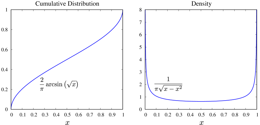
Figure 1: Cumulative distribution and density for the occupation time of the positive half line under Brownian motion.

3 Occupation times for quantum walks

When discussing occupation times for quantum walks one should decide when the walker will be “observed”, since this alters the natural evolution due to Born’s rule about quantum measurements. Here we consider a “monitoring” approach to occupation times similar to that one proposed in GVWW (13) and further considered in BGVW (14) to study recurrence in quantum walks. One should also look at KB (06).

This gives a natural way to look at the times when a coined or CMV quantum walk is on each half of the state space. The positive half consists of the span of the states

$$|0\rangle\otimes|\kern-3.3pt\downarrow\rangle\;,\;|1\rangle\otimes|\kern-3.3pt\uparrow\rangle\;,\;|1\rangle\otimes|\kern-3.3pt\downarrow\rangle\;,\;|2\rangle\otimes|\kern-3.3pt\uparrow\rangle\;,\;|2\rangle\otimes|\kern-3.3pt\downarrow\rangle\;,\;\dots$$ (5)

while the negative half consists of the span of the states

$$\dots\;,\;|-2\rangle\otimes|\kern-3.3pt\uparrow\rangle\;,\;|-2\rangle\otimes|\kern-3.3pt\downarrow\rangle\;,\;|-1\rangle\otimes|\kern-3.3pt\uparrow\rangle\;,\;|-1\rangle\otimes|\kern-3.3pt\downarrow\rangle\;,\;|0\rangle\otimes|\kern-3.3pt\uparrow\rangle$$ (6)

We call these the positive and the negative subspaces of our Hilbert state space respectively. In accordance with the setup in CGMV (10); BGVW (14), the orthogonal projection $P$ on the positive subspace plays a fundamental role in our results.

The monitoring approach assumes that a measurement is performed after each step to decide whether the walker is on the positive subspace or not. From a mathematical point of view, this results in the application of one of the projections, $P$ or $Q=I-P$, after the unitary step $U$ driving the evolution. While $P$ conditions on the event “the walker has been found on the positive subspace”, the complementary projection $Q$ conditions on the event “the walker has not been found on the positive subspace”. This gives the probability of any occupation distribution according to Born’s rule.

For example, if the walker starts at the state $\psi$, $\|\psi\|=1$, and runs for 6 steps, the quantity

$$\|PUPUQUPUQUPU\psi\|^{2}$$

gives the probability to find the walker on the positive subspace at times 1, 3, 5 and 6, but not at times 2 and 4. As a consequence, the probability of finding the walker, for instance, 2 times on the positive subspace, while running for a total number of 4 steps, is given by the sum

$$P(N_{4}=2)\quad= \,\|QUQUPUPU\psi\|^{2}+\|PUQUQUPU\psi\|^{2}$$

$$+ \,\|PUPUQUQU\psi\|^{2}+\|QUPUQUPU\psi\|^{2}$$

$$+ \,\|PUQUPUQU\psi\|^{2}+\|QUPUPUQU\psi\|^{2}.$$

The initial state in all our examples will be

$$\psi=\frac{1}{\sqrt{2}}\bigg{(}|0\rangle\otimes|\kern-3.3pt\uparrow\rangle+\imath\,|0\rangle\otimes|\kern-3.3pt\downarrow\rangle\bigg{)},$$

where $\iota$ is the imaginary unit.

More generally, the probability of finding the walker $r$ times on the positive subspace in the process of taking $n$ steps is given by the sum

$$P(N_{n}=r)\quad=\kern-3.0pt\sum_{\begin{subarray}{c}{P_{i}=P\,\text{or}\,Q}\\ P_{i}=P\text{ for }r\text{ indices}\end{subarray}}\kern-3.0pt\|(P_{n}U)\cdots(P_{2}U)(P_{1}U)\psi\|^{2}.$$

These quantities will be plotted against the relative number of steps $r/n$ in the graphics corresponding to the examples of the next sections. We will represent both, the “density” $P(N_{n}=r)$ and the “cumulative distribution” $P(N_{n}\leq r)=\sum_{k=0}^{r}P(N_{n}=k)$, which should be compared with Figure 1. Since we will be dealing with values of $n$ in the range $90$–$8100$ and $r$ between $0$ and $n$, it is clear that one needs a smart way to evaluate the sum given above—a direct approach would involve a prohibitive number of terms. Details on reducing the complexity of this calculation from $O(2^{n})$ to $O(n^{3})$ will be given in GVW .

The walker will evolve with a CMV walk with a doubly infinite CMV matrix that treats right and left “just the same”, to have a “fair” comparison with the classical case of a fair coin. Restricting for simplicity to real valued Verblunsky coefficients $\alpha_{i}$, we need to impose

$$\alpha_{i}=\alpha_{-2-i},\qquad i=0,1,2,3,\dots$$ (7)

a condition that leaves $\alpha_{-1}$ free. In the case of coined walks this amounts to taking real coins $C_{i}$ such that $C_{i}=C_{-1-i}$.

Our results, displayed in the next few sections, illustrate the fact that the quantum case gives us an embarrassment of riches, i.e. widely different behaviours can take place. All of them are unique to the quantum world, and yet some of them mimic the behaviour that most people expect in the classical case.

4 A look at the Hadamard walk

The first time that the occupation problem was considered for the Hadamard walk is Kon (12). This is a coined walk with constant coin

$$\frac{1}{\sqrt{2}}\begin{pmatrix}1&1\\ 1&-1\end{pmatrix}.$$ (8)

Although this coin is not of the form (2), such a form may be obtained after a change of phases in the basis CGMV (10, 12).

Our approach differs from the one in Kon (12), which needs an ad hoc normalization to get true probabilities due to the lack of a connection with a real measurement protocol. Therefore, for a finite number of steps our results do not agree. Nevertheless, we give some evidence that the limiting results apparently—and surprisingly—agree. Clarifying whether this coincidence holds by chance or there are good reasons for it is something that deserves future research.

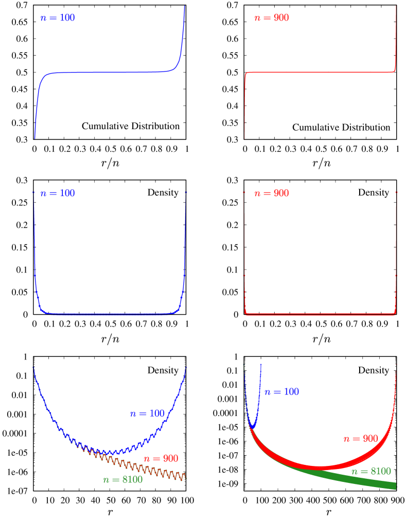
Figure 2: Cumulative distribution and density for $100$, $900$ and $8100$ steps of the Hadamard walk (monitoring approach).

The monitoring approach to occupation times in the Hadamard walk leads to the results shown in Figure 2, which plots the density and cumulative distributions for $100$, $900$ and $8100$ time steps. This figure points to a limiting distribution function given by two symmetric deltas at the edges of the interval. The take home message is that, in the limit of an infinite number of steps, the walker is always in the positive subspace or always in the negative subspace, each with probability $1/2$. More precisely, the discrete probabilities $P(N_{n}=r)$ appear to have a limit as $n\rightarrow\infty$ with $r$ held fixed,

$$P_{\infty}(r)=\lim_{n\rightarrow\infty}P(N_{n}=r)=\lim_{n\rightarrow\infty}P(N_{n}=n-r).$$ (9)

As seen in the bottom two panels of Figure 2, this limit has already nearly been reached for $0\leq r\leq 100$ by the time $n=900$. Indeed the $n=900$ result lies directly on top of the $n=8100$ result for $0\leq r\leq 100$. The numerical value of $P(N_{n}\leq 100\text{ or }N_{n}\geq n-100)$ with $n=900$ is $0.99994613$ while that of $n=8100$ is $0.99994530$. The reported digits with $n=8100$ appear to have stabilized, i.e. increasing $n$ further does not change the first eight digits of the probability. So if $n$ is a billion, the probability that the walker will be found on one side all but at most 100 times is $0.99994530$, and the fraction of the time it spends on the other side is $\leq 100/10^{9}$, effectively zero.

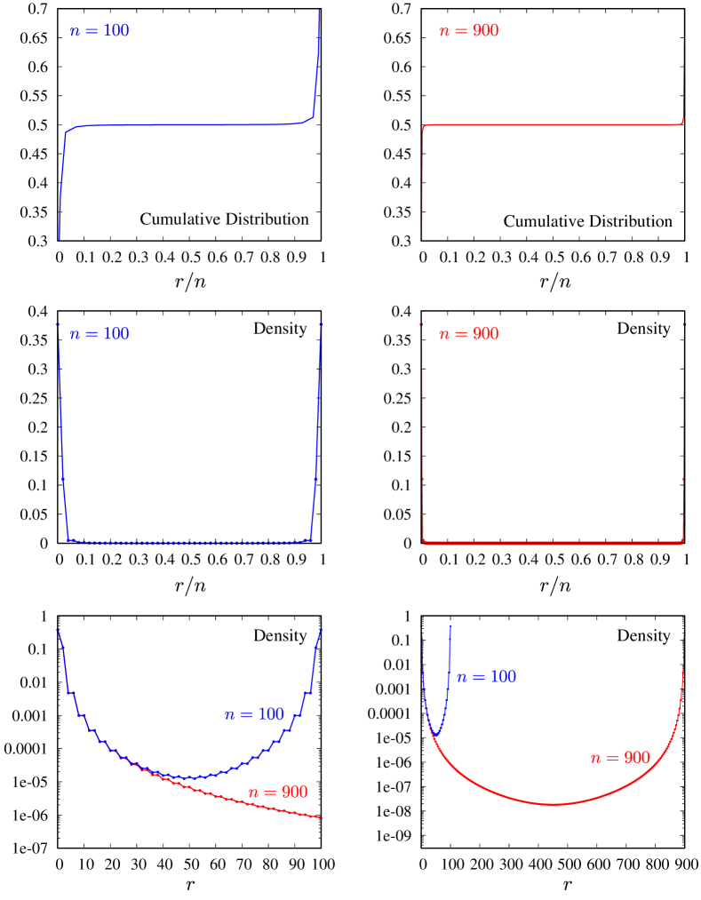
Figure 3: Cumulative distribution and density for $100$ and $900$ steps of the Hadamard walk (following Kon (12)).

Using the alternative definitions and approach in Kon (12) we have computed the density and the corresponding cumulative distribution for $n=100$ and $n=900$ steps of the Hadamard walk. The computation was too expensive to proceed past $n=900$. The setup is different, and only even values of $r$ lead to positive probabilities. Plots of the cumulative distribution and density (i.e. discrete probabilities) are given in Figure 3. This figure suggests the same limit distribution and behavior as the monitoring approach, though the values of $P_{\infty}(r)$ will be different.

5 The walk with a constant coin

In this section we deal with coined walks with a constant coin

$$C=\begin{pmatrix}\rho&-\alpha\\ \alpha&\;\rho\end{pmatrix},\qquad\alpha\in(-1,1),\qquad\rho=\sqrt{1-|\alpha|^{2}}.$$ (10)

Here we consider four different cases, corresponding to four choices of $\alpha$, namely $3/5$, $12/13$, $143/145$ and $399/401$. In each case the number of times steps is $120$. The plots for the occupation times using the monitoring approach are given in figures 4 and 5 below.

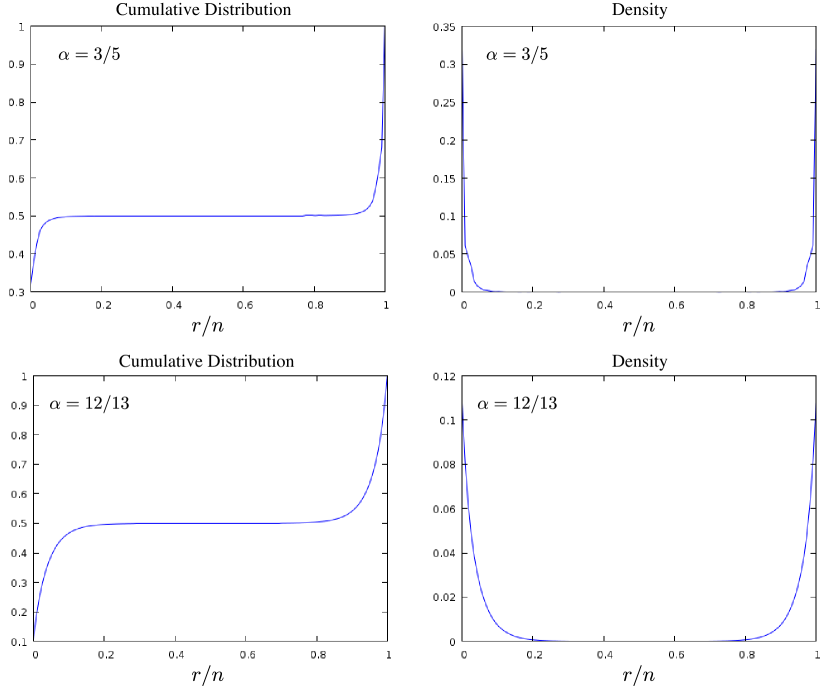
Figure 4: Cumulative distribution and density for the coin (10) with $\alpha=3/5$ and $\alpha=12/13$, both with 120 steps.

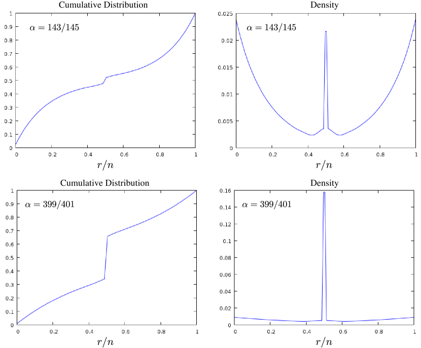
Figure 5: Cumulative distribution and density for the coin (10) with $\alpha=143/145$ and $\alpha=399/401$, both with 120 steps.

The message here is that for constant coins that are different from the Hadamard one the behaviour can differ substantially from that of the Hadamard case.

6 The even Verblunsky coefficients tend to one

In this section we look at a CMV walk whose Verblunsky coefficients $\alpha_{2i}\in(-1,1)$ depend on the site $i$, approaching the value $1$ as $|i|$ tends to infinity. For simplicity we take the odd Verblunsky coefficients to vanish, so as to have a coined walk with site dependent coins $C_{i}$ of the form (2) such that

$$C_{i}\quad\xrightarrow{|i|\to\infty}\quad C_{\infty}=\begin{pmatrix}0&-1\\ 1&\;0\end{pmatrix}.$$ (11)

The three different plots we show differ in the number of time steps. The plots are given in figure 6, and the effect of increasing the number of steps is to make the density more and more sharply concentrated around the value $1/2$.

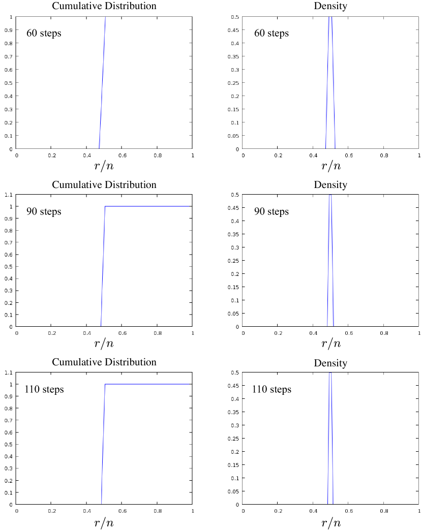
Figure 6: Cumulative distribution and density for $60$, $90$ and $110$ steps.

The take home message is that in the limit of an infinite number of steps, with probability $1$ the walker spends exactly half of the the time on the positive subspace and half on the negative subspace. In spirit, this is what most people feel the classical coin should be doing.

In this example, the Verblunsky coefficients are chosen to satisfy

$$\alpha_{2i-1}=0,\qquad\qquad\alpha_{2i}\;\xrightarrow{|i|\to\infty}\;1.$$

More explicitly, if $i$ is non-negative and even then

$$\alpha_{i}=\frac{(i+1)^{10}-1}{(i+1)^{10}+1},\qquad\qquad\rho_{i}=\frac{2(i+1)^{5}}{(i+1)^{10}+1},$$

and if $i$ is odd then $\alpha_{i}=0$ and $\rho_{i}=1$.

The corresponding CMV matrix $U$ is therefore a compact perturbation of the unitary matrix obtained by setting $\alpha_{2i-1}=0$ and $\alpha_{2i}=1$ in a CMV, which turns out to be a direct sum of the blocks $C_{\infty}$ in (11). As a consequence of Weyl’s theorem on the essential spectrum, the spectrum of $U$ accumulates on the eigenvalues $\pm i$ of $C_{\infty}$, so that it is pure point.

A couple of natural questions arise: Is the naive behaviour of occupation times observed in this example a common feature of any CMV walk with pure point spectrum? How does the occupation time distribution change when considering a CMV walk with other kind of singular spectrum?

While the first question remains as a challenge, in the next section we explore the second one.

7 A look at the Riesz walk

In this section we deal with the singular continuous measure constructed by F. Riesz Ri (1918), back in 1918. In GV (11) we study a purely singular continuous quantum walk in the non-negative integers naturally associated to it, by considering the semi-infinite CMV matrix generated by the Riesz measure. In this paper we consider an extension of this walk to the integers.

The measure on the unit circle that F. Riesz built is formally given by the expression

$$d\mu(z)=\prod_{k=1}^{\infty}(1+\cos(4^{k}\theta))\frac{d\theta}{2\pi}=\prod_{k=1}^{\infty}(1+(z^{4^{k}}+z^{-4^{k}})/2)\frac{dz}{2\pi iz}.$$ (12)

Here $z=e^{i\theta}$. If one truncates this infinite product the corresponding measure has a nice density. These approximations converge weakly to the Riesz measure.

The construction of this example is based on detailed knowledge of the coefficients $\alpha_{i}$, $i\geq 0$, for the Riesz measure which are found in GV (11). We define a “Riesz walk” on the integers as a a CMV walk defined by extending the Verblunsky coefficients of the Riesz measure to negative indices according to the “fair” rule (7).

This example is of interest since it is not clear that a “limit law” exists for the “site distribution” of the Riesz walk on the positive half of the integers, see GV (11). The same issue arises when one looks at the walk on the integers. The existence of such a limit law for the case of a constant coin is discussed in Kon (08).

Figure 7 shows the density and cumulative distribution for 90 steps of the Riesz walk on the integers.

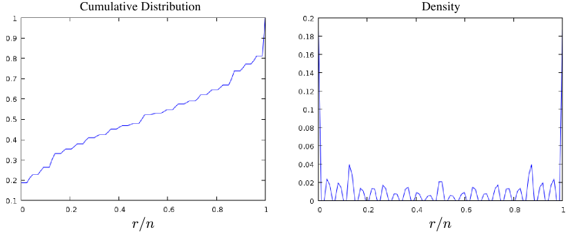
Figure 7: Cumulative distribution and density for 90 steps of Riesz’s walk.

These examples open up many interesting questions: What can be said in general about the occupation time distribution in CMV walks? Is there any spectral characterization for the different behaviours of such distributions? Is the connection with orthogonal polynomials on the unit circle useful for such a characterization? In particular, is there any important role reserved for the Schur functions in this respect? The last question is motivated by the central role played by Schur functions in both, the theory of orthogonal polynomials on the unit circle Sim05a ; Sim05b , and the study of quantum walks GVWW (13); BGVW (14); CGMV (12); GV (18); GLV (20); CGGV (19).

References

- ADZ (93) Y. Aharonov, L. Davidovich, N. Zagury, Quantum random walks, Phys. Rev. A 48 (1993), 1687–1690.
- BGVW (14) J. Bourgain, F. A. Grünbaum, L. Velázquez, J. Wilkening, Quantum recurrence of a subspace and operator-valued Schur functions, Comm. Math. Phys. 329 (2014), 1031–1067.
- CGMV (10) M. J. Cantero, F. A. Grünbaum, L. Moral, L. Velázquez, Matrix valued Szegő polynomials and quantum random walks, Commun. Pure Appl. Math. 58, (2010) 464–507.
- CGMV (12) M. J. Cantero, F. A. Grünbaum, L. Moral, L. Velázquez, The CGMV method for quantum walks, Quantum Inf. Process. 11 (2012), 1149–1192.
- CMV (03) M. J. Cantero, L. Moral, L. Velázquez, Five-diagonal matrices and zeros of orthogonal polynomials on the unit circle, Linear Algebra Appl. 362 (2003), 29–56.
- CGGV (19) C. Cedzich, T. Geib, F. A. Grünbaum, L. Velázquez, A. H. Werner, R. F. Werner, Quantum walks: Schur functions meet symmetry protected topological phases, arXiv:1903.07494, 18 Mar 2019.
- CF (49) K. L. Chung, W. Feller, On fluctuations in coin-tossing, PNAS 35 (1949), 605–609.
- ES (17) P. Ernst, L. Shepp, On occupation times of the first and third quadrants for planar Brownian motion, J. Appl. Prob. 54 (2017), 337–342
- Fel (68) W. Feller, An introduction to probability theory and its applications, vol. 1, J. Wiley & Sons, Inc. 1968.
- Gr (18) F. A. Grünbaum, A Feynman-Kac approach to a paper of Chung and Feller on fluctuations in the coin-tossing game, PAMS (2020), to appear, arXiv:1810.06092v1, 14 Oct 2018.
- GLV (20) F. A. Grünbaum, C. Lardizabal, L. Velázquez, Quantum Markov Chains: Recurrence, Schur Functions and Splitting Rules, Ann. Henri Poincaré 21 (2020), 189–239.
- GG (07) F. A. Grünbaum, C. McGrouther, Occupation time for two dimensional Brownian motion in a wedge, Proceedings of Symposia in Applied Mathematics, vol. 65, (2007).
- GV (11) F. A. Grünbaum, L. Velázquez, The quantum walk of F. Riesz, Foundations of computational mathematics (Budapest, 2011), pp. 93–112, London Math. Soc. Lecture Note Ser. 403, Cambridge Univ. Press, Cambridge, 2013.
- GV (18) F. A. Grünbaum, L. Velázquez, A generalization of Schur functions: Applications to Nevanlinna functions, orthogonal polynomials, random walks and unitary and open quantum walks, Adv. Math. 326 (2018), 352–464.
- (15) F. A. Grünbaum, L. Velázquez, J. Wilkening, Occupation times for quantum walks, (manuscript in preparation).
- GVWW (13) F. A. Grünbaum, L. Velázquez, A. H. Werner, R. F. Werner, Recurrence for discrete time unitary evolutions, Comm. Math. Phys. 320 (2013), 543–569.
- Kac (51) M. Kac, On some connections between probability theory and differential and integral equations, Proc. Second Berkeley Symposium on Math. Stat. and Probability, Univ. of Calif. Press, 1951, pp. 189–215.
- Kem (03) J. Kempe, Quantum random walks-an introductory overview, Contemporary Physics 44, No. 4 (2003), 307–327.
- Kon (08) N. Konno, Quantum walks, in Quantum Potential Theory, U. Franz, M. Schürmann, editors, Lecture notes in Mathematics 1954, Springer Verlag, Berlin Heidelberg, 2008.
- Kon (12) N. Konno, Sojourn times of the Hadamard walk in one dimension, Quantum Inf. Process 11, (2012), 465–480.
- Kon (11) N. Konno, E. Segawa, Localization of discrete-time quantum walks on a half line via the CGMV method, Quantum Inf. Comput. 11 (2011), 485–495.
- KS (14) N. Konno, E. Segawa, One-dimensional quantum walks via generating function and the CGMV method, Quantum Inf. Comput. 14 (2014), 1165–1186.
- KB (06) H. Krovi, T. Brun, Hitting time for quantum walks on the hypercube, Phys. Rev. A 73 (2006), 032341.
- Lev (39) P. Lévy, Sur certains processus stochastiques homogenes, Compositio Math. 7 (1939), 283–339.
- McK (14) H. P. McKean Jr., Probability theory, the classical limit theorems, Cambridge University Press, 2014.
- Ren (60) A. Renyi, Legendre polynomials and probability theory, Ann. Univ. Sci. Budapest, Eötvös Sect. Math 3-4, 1960-1961, 247–251.
- Ri (1918) F. Riesz, Über die Fourierkoeffizienten einer stetigen Funktion von beschränkter Schwankung, Math. Z. 18 (1918), 312–315.
- (28) B. Simon, Orthogonal Polynomials on the Unit Circle, Part 1: Classical Theory, AMS Colloq. Publ., vol. 54.1, AMS, Providence, RI, 2005.
- (29) B. Simon, Orthogonal Polynomials on the Unit Circle, Part 2: Spectral Theory, AMS Colloq. Publ., vol. 54.2, AMS, Providence, RI, 2005.
- Str (93) D. Stroock, Probability Theory, an analytical view, Cambridge University Press, 1993.