Impact of laser polarization on q-exponential photon tails in non-linear Compton scattering

Abstract

Non-linear Compton scattering of ultra-relativistic electrons traversing high-intensity laser pulses generates also hard photons. These photon high-energy tails are considered for parameters in reach at the forthcoming experiments LUXE and E-320. We consider the invariant differential cross sections $d\sigma/du$ between the IR and UV regions and analyze the impact of the laser polarization and find q-deformed exponential shapes. (The variable $u$ is the light-cone momentum-transfer from initial electron to final photon.) Optical laser pulses of various durations are compared with the monochromatic laser beam model which uncovers the laser intensity parameter in the range $\xi=1\cdots 10$. Some supplementary information is provided for the azimuthal final-electron/photon distributions and the photon energy-differential cross sections.

I Introduction

The planned experiments LUXE at DESY Abramowicz:2019gvx ; Abramowicz:2021zja ; Altarelli:2019zea ; Hartin:2018sha and E-320 at FACET-II E_320 aim at studying fundamental QED processes within strong laser fields characterized by intensities in the order of $10^{20}$ W/cm². A particular feature is the use of a high-quality electron ($e^{-}$, mass $m$, charge $-|e|$) beam provided by an accelerator, thus possessing fairly well controlled parameters. The available beams uncover ultra-relativistic energies $E_{e^{-}}=10\cdots 50$ GeV. Even for non-ultra-strong lasers in the so-called transition region in between weak-field and strong-field limits of QED, the field strength, which the electron experiences in its local rest system, reaches values in the order of the so-called (critical) Sauter-Schwinger electric field ${\cal E}_{crit}=m^{2}/|e|\approx 1.3\times 10^{18}$ V/m, thus enabling a test of strong-field QED in a hitherto less explored regime and continuing the seminal experiments Bula:1996st ; Burke:1997ew ; Bamber:1999zt ; Poder:2018ifi ; Cole:2017zca towards the precision regime. For an introduction to the state-of-the-art physics case of strong-field QED and a deeper survey on quantum processes in strong e.m. fields, we refer the interested reader to the theory sections in Abramowicz:2021zja together with Abramowicz:2019gvx ; Altarelli:2019zea ; Hartin:2018sha ; E_320 ; Turcu:2016dxm ; Meuren:2020nbw .

When considering electron-laser interactions, e.g. the nonlinear Compton scattering as the Furry picture process $e_{L}(p)\to e_{L}(p^{\prime})+\gamma(k^{\prime})$, where $e_{L}$ stands for the laser-dressed electron and $\gamma$ for the emitted photon, two invariant parameters are often used in plane-wave backgrounds to characterize the entrance channel Ritus ; DiPiazza:2011tq :

$$\xi = \frac{ea}{m},$$ (1)

$$\chi = \xi\frac{k\cdot p}{m^{2}},$$ (2)

where $a$ is the amplitude of electromagnetic potential and momentum four-vectors $k$, $k^{\prime}$ and $p$ refer to the laser-beam wave-vector, the $out$-photon (with energy $\omega^{\prime}$), and the $in$-electron, respectively. The $out$-electron four-momentum is $p^{\prime}$. The invariant laser intensity parameter in the lab. system reads $\xi=(m/\omega)({\cal E}/{\cal E}_{crit})$. The meaning of the parameter $\chi$ becomes more transparent in the electron’s rest system:

$$\chi=\frac{\cal E}{{\cal E}_{crit}}\left(\frac{E_{e^{-}}}{m}+\sqrt{\frac{E_{e^{-}}^{2}}{m^{2}}-1}\right)\bigg{\rvert}_{E_{e^{-}}=m}=\frac{\cal E}{{\cal E}_{crit}}\leavevmode\nobreak\ .$$ (3)

The frequency of a Ti:Sapphire laser is $\omega=1.55$ eV, thus $m/\omega\gg 1$. In other words, even for lasers with intensities $\xi\gtrsim 1$, i.e. ${\cal E}/{\cal E}_{crit}\ll 1$ in the lab., the Lorentz boost of the electric field strength ${\cal E}$ lets the quantum parameter become $\chi\lesssim 1$, thus testing the sub-critical up to the critical regime, ${\cal E}\lesssim{\cal E}_{crit}$ for $E_{e^{-}}=17.5$ GeV in the electron’s rest system.

Among the options at LUXE and E-320 are investigations of non-linear effects in Compton scattering, Breit-Wheeler pair production and trident pair production. Here, we consider non-linear Compton scattering as one-photon emission by an electron traversing a laser pulse. We focus on the photon tails: the region beyond the Klein-Nishina edge, i.e. excluding the IR region, and prior to the kinematic limit, i.e. excluding the UV region towards the kinematical limit. The considered laser intensities $\xi\sim 1$ are in between weak-field and strong-field limits, where approximation schemes are often hardly universally applicable. ( Among important approximation schemes are the locally constant field approximation Harvey:2014qla and improvements Ilderton:2018nws ; DiPiazza:2017raw ; DiPiazza:2018bfu and the locally monochromatic approximation scheme Heinzl:2020ynb as well.)

It was already noted by Ritus Ritus that non-linear Compton scattering for circular laser polarization is fundamentally different from linear polarization. One may expect this: The classical trajectory of a point-like charge in a circularly polarized e.m. wave is essentially on a circle perpendicular to the wave vector $\vec{k}$, while in a linearly polarized e.m. wave it is on the figure-8 curve in direction of $\vec{k}$ and parallel to the polarization vector $\vec{a}$. Correspondingly, the radiation patterns of the moving charges are expected to differ. In fact, in a monochromatic plane wave, the circular polarization facilitates the dead cone effect Titov:2019kdk ; Harvey:2009ry ; Maltoni:2016ays , i.e. all harmonics beyond the first one are zero for on-axis back-scattering, while for the linear polarization only the even harmonics are zero, which is a clear manifestation of specific properties of transition matrix elements described by their distinct basic functions.

We are going to compare the photon tails in non-asymptotic regions of $\xi$ and $u=k\cdot k^{\prime}/(k\cdot p-k\cdot k^{\prime})$ for circular and linear polarizations. Such comparative studies appeared already in the recent literature, e.g. Titov:2019kdk ; Heinzl:2020ynb , but not with emphasis on the intermediate photon tails. The tails in the considered region display a q-deformed exponential shape of the invariant cross sections $d\sigma/du$, which we quantify accordingly. We also show that the monochromatic laser model is a useful reference, supported by numerical results of laser pulses when considering the differential spectra $d\sigma/du$ or $d\sigma/d\omega^{\prime}$.

Our note is organized as follows. In section II we recall the basic formulas of one-photon emission by electrons in laser pulses and in a monochromatic laser beam and in a constant cross field; we also supply certain limits of these formulas. The central part, section III, is devoted to the numerical evaluation of these less transparent formulas. There, we also comment on the azimuthal distribution $d^{2}\sigma/du\,d\phi_{e^{\prime}}$ of the recoil electron described by the four-momentum $p^{\prime}$. In section IV, we describe the adjustment of q-exponentials to the $u$-differential cross sections. The discussion in section V is devoted to integrated cross sections with cut-off, some remarks on emissivity of thermalized systems and the relation of the spectra $d\sigma/du$ vs. $d\sigma/d\omega^{\prime}$. We conclude in section VI.

II Basics

The here considered process of non-linear Compton scattering (cf. DiPiazza:2020wxp ; Seipt:2020diz ; Valialshchikov:2020dhq for recent developments and detailed citations) is the Furry-picture one-photon emission by an electron traversing an external electromagnetic field which approximates the laser on different levels of sophistication. This section recaps the used formulas in the subsequent numerical analysis.

II.1 Laser pulses

The laser pulse model for plane waves is described by the four-potential in axial gauge, $A^{(i)}=(0,\vec{A}^{(i)})$, with

$$\vec{A}^{(i)}=f(\phi)\left(\vec{a}_{x}(i)\cos\phi+\vec{a}_{y}(i)\sin\phi\right)$$ (4)

where $\vec{a}_{x}(circ)^{2}=\vec{a}_{y}(circ)^{2}=\vec{a}_{x}(lin)^{2}=m^{2}\xi^{2}/e^{2}$, and $\vec{a}_{y}(lin)^{2}=0$; the polarization vectors $\vec{a}_{x}(circ)$ and $\vec{a}_{y}(circ)$ are mutually orthogonal. The intensity parameter $\xi$ is considered henceforth as independent invariant variable characterizing the laser. The mean energy densities $\propto\langle A^{2}\rangle$ differ therefore by a factor of two for circular and linear polarizations at given value of $\xi$. We ignore a possible non-zero value of the carrier envelope phase and focus on symmetric envelope functions $f(\phi)$ w.r.t. the invariant phase $\phi=k\cdot x$.

We recall the formalism of Titov:2019kdk to display the relevant equations for the calculation of the differential cross sections for circular ($i=circ$) and linear ($i=lin$) polarizations:

$$\frac{d\sigma^{(i)}}{du}=\frac{\alpha^{2}}{\xi^{2}N^{(i)}}\frac{1}{k\cdot p}\frac{1}{(1+u)^{2}}\int_{0}^{2\pi}d\phi_{e^{\prime}}\int_{\ell_{\rm min}}^{\infty}d\ell\,w^{(i)}(\ell),$$ (5)

where $\ell_{\rm min}=um^{2}/2(k\cdot p)$ and

$$w^{(i)}(\ell)=\left\{\begin{array}[]{l}-2|\tilde{Y}_{\ell}|^{2}\,+\,\xi^{2}\left(1+\frac{u^{2}}{2(1+u)}\right)\left(|Y_{\ell-1}|^{2}+|Y_{\ell+1}|^{2}-2\mbox{Re}\tilde{Y}_{\ell}X_{\ell}^{*})\right)\,\mbox{for}\,i=circ,\\ -2|\tilde{A}_{0}|^{2}+2\xi^{2}\left(1+\frac{u^{2}}{2(1+u)}\right)\left(|\tilde{A}_{1}|^{2}-\mbox{Re}\tilde{A}_{0}\tilde{A}_{2}^{*}\right)\,\mbox{for}\,i=lin\leavevmode\nobreak\ .\end{array}\right.$$ (6)

The Lorentz and gauge invariant quantity squared $\xi^{2}$ is the classical non-linearity parameter characterizing solely the laser beam, and $\alpha$ stands for the fine-structure constant. The above defined invariant $u=k\cdot k^{\prime}/k\cdot p^{\prime}$ is used to characterize the $out$-photon. The normalization factors $N^{(i)}$, which are related to the average density of the e.m. field $\langle\cal{E}\rangle$, are expressed through the envelope functions as

$$N^{(i)}_{0}=\frac{1}{2\pi}\int\limits_{-\infty}^{\infty}d\phi\left(f^{2}(\phi)+{f^{\prime}}^{2}(\phi)\right)\times\left\{\begin{array}[]{l}1\,\mbox{for}\,i=circ,\\ \cos^{2}(\phi)\ \,\mbox{for}\,i=lin,\\ \end{array}\right.$$ (7)

with the asymptotic values $N^{(circ)}_{0}\simeq\Delta/\pi$ and and $N^{(lin)}_{0}\simeq\Delta/2\pi$ at $\Delta/\pi\gg 1$. The functions $Y_{\ell},X_{\ell}$ and $\tilde{Y}_{\ell}$ are defined by

$$Y_{\ell}(z) = \frac{1}{2\pi}{\rm e}^{-i\ell(\phi_{e^{\prime}})}\int\limits_{-\infty}^{\infty}\,d\phi\,{f}(\phi)\,{\rm e}^{i\ell\phi-i{\cal P}^{(circ)}(\phi)}\leavevmode\nobreak\ ,$$

$$X_{\ell}(z) = \frac{1}{2\pi}{\rm e}^{-i\ell(\phi_{e^{\prime}})}\int\limits_{-\infty}^{\infty}\,d\phi\,{f^{2}}(\phi)\,{\rm e}^{i{\ell}\phi-i{\cal P}^{(circ)}(\phi)}\leavevmode\nobreak\ ,$$

$$\widetilde{Y}_{\ell}(z) = \frac{z}{2l}\left[Y_{\ell+1}(z)+Y_{\ell-1}(z)\right]-\xi^{2}\frac{u}{u_{l}}\,X_{\ell}(z)\leavevmode\nobreak\ ,$$ (8)

where $\phi_{e^{\prime}}$ is the azimuthal angle of the $out$-electron $u_{\ell}={2\ell(k\cdot p)}/{m^{2}}$ and

$${\cal P}^{(circ)}(\phi) = z\int\limits_{-\infty}^{\phi}\,d\phi^{\prime}\,f(\phi^{\prime})\cos(\phi^{\prime}-\phi_{e^{\prime}})-\frac{\xi^{2}m^{2}u}{2(k\cdot p)}\int\limits_{-\infty}^{\phi}\,d\phi^{\prime}\,f^{2}(\phi^{\prime})\leavevmode\nobreak\ .$$ (9)

The functions $\widetilde{A}_{m}(\ell)$ for $m=1,2$ read

$$\widetilde{A}_{m}(\ell)=\frac{1}{2\pi}\int\limits_{-\infty}^{\infty}d\phi\,f^{m}(\phi)\cos^{m}(\phi)\,{\rm e}^{i\ell\phi-i{\cal P}^{(lin)}(\phi)}\leavevmode\nobreak\ ,$$ (10)

$${\cal P}^{(lin)}(\phi) = \tilde{\alpha}(\phi)-\tilde{\beta}(\phi)\leavevmode\nobreak\ ,$$ (11)

$$\tilde{\alpha}(\phi) = \hat{\alpha}\int\limits_{-\infty}^{\phi}d\phi^{\prime}f(\phi^{\prime})\cos(\phi^{\prime})\leavevmode\nobreak\ ,\quad\hat{\alpha}=z\cos\phi_{e^{\prime}}$$ (12)

$$\tilde{\beta}(\phi) = 4\hat{\beta}\int\limits_{-\infty}^{\phi}d\phi^{\prime}f^{2}(\phi^{\prime})\cos^{2}(\phi^{\prime})\leavevmode\nobreak\ ,\quad\hat{\beta}=\frac{u\xi^{2}m^{2}}{8k\cdot p}\leavevmode\nobreak\ ,$$ (13)

and the function $\widetilde{A}_{0}(\ell)$ follows from the identity Titov:2019kdk

$$\ell\widetilde{A}_{0}(\ell)-\hat{\alpha}\widetilde{A}_{1}(\ell)+4\hat{\beta}\widetilde{A}_{2}(\ell)=0\leavevmode\nobreak\ .$$ (14)

All basis functions have the arguments $z=z_{\ell}={2\ell\xi}\sqrt{\frac{u}{u_{\ell}}(1-\frac{u}{u_{\ell}})}$ and are defined for $0\leq u\leq u_{\ell}$ vanishing elsewhere. Note the correspondence with the analog expressions for the monochromatic model below, where the discrete harmonic number $n$ appears instead of the internal continuous variable $\ell$.

II.2 Special: monochromatic laser beam model

A monochromatic laser field in plane-wave approximation is described by Eq. (4) with $f(\phi)=1$. The invariant differential cross sections for one-photon emission read Ritus :

$$\frac{d\sigma^{(i)}_{IPA}}{du}=\frac{\alpha^{2}}{\xi^{2}}\frac{1}{(k\cdot p)\,N^{(i)}}\frac{1}{(1+u)^{2}}\sum_{n=1}^{\infty}\int_{0}^{2\pi}d\phi_{e^{\prime}}\,F_{n}^{(i)}(z_{n}),$$ (15)

where $N^{(circ)}=1$ and $N^{(lin)}=\frac{1}{2}$ and

$$F_{n}^{(i)}=\left\{\begin{array}[]{l}-2J_{n}(z_{n})^{2}+\xi^{2}\left(1+\frac{u^{2}}{2(1+u)}\right)\left(J_{n+1}(z_{n})^{2}+J_{n-1}(z_{n})^{2}-2J_{n}(z_{n})^{2}\right)\quad\mbox{for}\,i=circ,\\ -2A_{0}^{2}+2\xi^{2}\left(1+\frac{u^{2}}{2(1+u)}\right)(A_{1}^{2}-A_{0}A_{2})\quad\mbox{for}\,i=lin,\end{array}\right.$$ (16)

for $0\leq u\leq u_{n}$ and $F_{n}^{(i)}=0$ elsewhere. $J_{n}$ are Bessel function of the first kind (independent of the $out$-electron azimuthal angle $\phi_{e^{\prime}}$), and the functions $A_{m}(z_{n})$, $m\in 0,1,2$, are defined by

$$A_{m}(n,\hat{\alpha},\hat{\beta})=\frac{1}{2\pi}\int_{-\pi}^{\pi}d\phi\cos^{m}(\phi)\cos(n\phi-\hat{\alpha}\sin\phi+\hat{\beta}\sin 2\phi),$$ (17)

where $\hat{\alpha}=z_{n}\cos\phi_{e^{\prime}}$ and $\hat{\beta}=\frac{\xi^{2}um^{2}}{8k\cdot p}$. The arguments are $z_{n}(u,u_{n})=\frac{2n\xi}{\sqrt{1+c_{i}\xi^{2}}}\sqrt{\frac{u}{u_{n}}(1-\frac{u}{u_{n}})}$ with $u_{n}=\frac{2nk\cdot p}{m^{2}(1+c_{i}\xi^{2})}$ with $c_{circ}=1$ and $c_{lin}=\frac{1}{2}$. The effective masses $m^{2}(1+c_{i}\xi^{2})$ and their role in the (quasi-) momentum balance as well as the relation to asymptotic four-momenta ($p/p^{\prime}$ for $in/out$-electrons and $k/k^{\prime}$ for $in/out$-photons) are discussed in detail in LL ; Harvey:2009ry . The differential non-linear Compton cross section for circular polarization has been used fairly often as standard reference LL ; Harvey:2009ry . We use the label IPA as acronym of “infinite pulse approximation”.

The large-$\xi$ limit of Eq. (15) reads (cf. Ritus )

$$\frac{d\sigma^{(i)}_{IPA,large-\xi}}{du} = \frac{8\alpha^{2}}{\pi^{b_{(i)}}\,\xi^{2}(k\cdot p)\,N^{(i)}}\frac{1}{(1+u)^{2}}\int\limits_{0}^{\pi}d\psi\int\limits_{-\infty}^{\infty}d\tau$$ (18)

$$\times v_{(i)}^{\frac{1}{3}}[-\Phi^{2}(y_{(i)})+v_{(i)}^{-\frac{2}{3}}\left(1+\frac{u^{2}}{2(1+u)}\right)(y\Phi^{2}(y_{(i)})+{\Phi^{\prime}}^{2}(y_{(i)}))]$$

with Airy function $\Phi$ and its derivative $\Phi^{\prime}$ and $y_{(i)}=(1+\tau^{2})v_{(i)}^{\frac{2}{3}}$ and $v_{(i)}=u/(2\chi S^{(i)})$, where

$$S^{(i)}=\left\{\begin{array}[]{l}1\quad\mbox{for}\,i=circ,\\ \sin\psi\quad\mbox{for}\,i=lin,\end{array}\quad\quad\right.b^{(i)}=\left\{\begin{array}[]{l}1\quad\mbox{for}\,i=circ,\\ 2\quad\mbox{for}\,i=lin.\end{array}\right.$$ (19)

The expressions for circular and linear polarizations look similar. The principle difference is that the mod-square of the matrix element, in the case of circular polarization, does not depend on the azimuthal angle of the outgoing particle. This leads to a one-dimensional integral, in contrast to a two-dimensional integral over auxiliary variables $\psi$ and $\tau$ in the case of linear polarization. Formally, the corresponding cases are related by $lin\to circ$ via

$$N^{lin}\to N^{circ},\qquad\psi=\frac{\pi}{2},\qquad\int\limits_{0}^{\pi}d\psi\to\pi\leavevmode\nobreak\ .$$ (20)

II.3 Constant cross field

The asymptotic cross section for circular polarization in the large-$\xi$ limit, $d\sigma^{(circ)}_{IPA,large-\xi}/du$, Eq. (18), coincides with the one-photon emission in a constant cross field (ccf) Ritus :

$$\frac{d\sigma_{ccf}}{du} = -\frac{4\pi\alpha^{2}}{m^{2}\xi}\frac{1}{\chi}\frac{1}{(1+u)^{2}}\left(\int_{z}^{\infty}dy\,\Phi(y)+\frac{2}{z}\left[1+\frac{u^{2}}{2(1+u)}\right]\Phi^{\prime}(z)\right)$$ (21)

$$\stackrel{{\scriptstyle u\gg 1,\chi}}{{\longrightarrow}} \simeq \frac{2\sqrt{\pi}\alpha^{2}}{m^{2}\xi}\chi^{-1/2}u^{-3/2}\exp\left(-\frac{2u}{3\chi}\right),$$ (22)

where the last line is the large-$u$ approximation, denoted hereafter as $d\sigma_{ccf,large-u}/du$. $\Phi(z)$ and $\Phi(z)^{\prime}$ stand again for the Airy function and its derivative with arguments $z=(u/\chi)^{2/3}$.

III Numerical results

The following numerical results are for parameters motivated by LUXE Abramowicz:2019gvx ; Abramowicz:2021zja : $E_{e^{-}}=17.5$ GeV and $\omega=1.55$ eV for the idealized case of a head-on collision, meaning $k\cdot p/m^{2}=0.2078$ in the entrance channel. To specify the laser model (4), we employ $f(\phi)=1/\cosh(\phi/\pi N)$, where $N$ characterizes the number of oscillations in the pulse. The typical pulse duration of the envisaged experiments is $T\approx 30$ fs which corresponds to the number of cycles in a pulse $N\approx T\omega/(2\pi)\approx 10$. In view of the general physical interest and for methodological purposes, we extended our consideration to the region of ultra-short (sub-cycle) and short pulses with $1\leq N\leq 10$. Results for circular and linear polarizations are compared at given value of $\xi$.

III.1 Invariant cross sections $d\sigma/du$

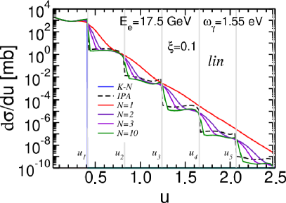
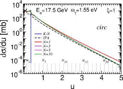
Figure 1: Invariant differential cross sections $d\sigma^{(i)}/du$ for $\xi=0.1$ (top panels) and for $\xi=1$ (bottom panels). The solid curves are for ultra-short and short laser pulses with envelope function $f(\phi)=1/\cosh(\phi/(\pi N))$ for various values of $N=1,3,5$ and 10 as given by the legends (the $N=10$ curves are on top of the $N=3$, 5 curves in the used scale). The dashed curves are for the monochromatic laser beam model $d\sigma^{(i)}_{IPA}/du$ (15). The solid blue curve depicts the Klein-Nishina (K-N) cross section $d\sigma_{IPA}/du|_{\xi\to 0}$. The gray vertical grid lines in top panels and gray combs in bottom panels display the IPA harmonic positions $u_{n}$. Left panels: circular polarization, right panels: linear polarization.

Let us consider the above pulse envelope function $f(\phi)=1/\cosh(\phi/(\pi N))$ to elucidate the impact of a finite pulse duration and contrast it later on with the monochromatic laser beam model and some approximations thereof. Differential spectra $d\sigma/du$ are exhibited in Fig. 1. The panels in the top row are for a low field intensity, $\xi=0.1$. In this case, our model manifests a significant sensitivity of cross sections to the pulse duration parameterized by $N$. Most notable is the dependence on the laser polarization: For circular polarization (left top panel), the harmonic structures, which arise when crossing the respective upper limit $u_{\ell,n}$ of a certain harmonic, are rather modest, while for linear polarization (right top panel) they persist in a much more pronounced manner up to larger values of the variable $u$. The monochromatic model (15) (note some even-odd modification of peaked structures to smooth ones at the respective harmonic thresholds $u_{n}$ for linear polarization, in particular for $\xi=0.1$) reproduces the pulse model (5) fairly well for longer pulses. Note that, in the partial probabilities of a sub-cycle pulse with $N=1$ or smaller, an effective high-energy component in the Fourier spectrum of the laser pulse is generated, which leads to a significant increase of the corresponding cross sections/probabilities. When the duration of a pulse increases this effect decreases and the enhancement vanishes Titov:2012rd . One can see a qualitative agreement between results for infinite pulses and finite pulses with $N=10$. Some visible difference between them is explained by the quite different basic functions, say Bessel functions for IPA and functions (8), for circular polarization. This difference is much smaller than the scale of variation of the cross sections in the range $0<u<5$ which is many orders of magnitude.

Ultra-short pulses, e.g. $N=1$ exhibit hardly the harmonic structures, both for circular and linear polarizations, in particular at larger values of $u$. Such a pulse duration dependence fades away considerably at the higher intensity $\xi=1$ exhibited in the bottom panels. Focusing first on circular polarization (see left bottom panel) and the region $u>0.5$, one observes a structureless and smooth spectrum with a tiny dependence on the pulse duration for $N>1$. Only the ultra-short pulse result with $N=1$ is lifted at large values of $u$. Taking the monochromatic model as reference, one recognizes the approach of the $N>1$ results to it at large values of $u$. Only at $u\lesssim 3$, the monochromatic model falls somewhat short (a factor up to about three) in relation to the pulse results. The difference in cross sections $d\sigma^{(i)}/du$ with $N=3\cdots 10$ is comparable to the line thickness of the curves and is not visible at the given scale.

The dependence on the pulse duration for linear polarization is also weak (see right bottom panel of Fig. 1). The short pulses, $N=3$, 5 and 10, carry a weak remainder of the harmonic structures up to large values of $u$. For the ultra-short pulse, $N=1$, the spectrum is completely smooth beyond the Klein-Nishina edge, similar to the circularly polarized laser pulse. The spectra are somewhat steeper than the ones for circular polarization. The monochromatic model, in contrast, displays pronounced harmonic structures up to large values of $u$. Remarkably, in the range of our interest, $u\in[0.5,4]$, the pulse model results are represented nicely by the smoothed monochromatic model. We conclude that, for the gross features, the monochromatic model provides a good guidance for the tails of the spectra $d\sigma^{(i)}/du$ beyond the stark harmonic structures at small values of $u$, which extend roughly up to the Klein-Nishina edge. The occurrence of the photon tails beyond the Klein-Nishina edge, $u>u_{K-N}=0.416$, is a clear signature of the multi-photon effects, becoming operative in intense lasers, both for circular and linear polarizations.

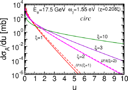
Figure 2: Invariant differential cross sections, based on an expression derived for asymptotically large field intensity $d\sigma^{(i)}_{A}/du\equiv d\sigma^{(i)}_{IPA,large-\xi}/du$, Eq. (18), for $\xi=1,2,3,10$ (solid curves). For a comparison, the dashed curves with labels IPA ($\xi=1$ and 2) are for the monochromatic laser beam model $d\sigma^{(i)}_{IPA}/du$, Eq. (15). Left panel: circular polarization, right panel: linear polarization.

Given the proximity of the spectra for laser pulses with the monochromatic model, we consider now the change of the spectral shapes with increasing values of the laser intensity $\xi$. We employ the large-$\xi$ approximation Eq. (18). As seen in Fig. 2, this approximation is useful already for $\xi=2$ and not too bad for $\xi=1$. Of course, the harmonic structures for linear polarization are not captured by Eq. (18), which is not problematic when considering the gross features of the spectra beyond the Klein-Nishina edge. Interestingly, the harmonic structures for the case of linear polarization persist from the small-$u$ region up to large values of $u$ for $\xi\lesssim 2$, see right panel of Fig. 2. The harmonic structures fade away for $\xi>2$. The overall pattern resembles on first sight the one for the above circular polarization case.

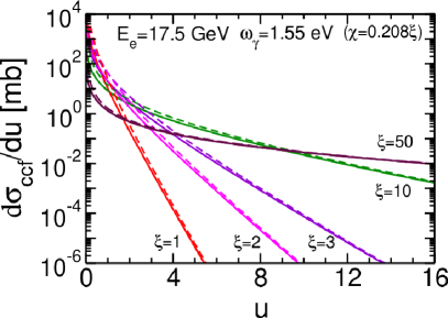
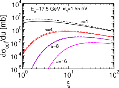
Figure 3: Comparison of constant cross field results of $d\sigma_{ccf}/du$, Eq. (21), (solid curves) and $d\sigma_{ccf,large-u}/du$, Eq. (22), (dashed curves). Note that the large-$\xi$ approximation $d\sigma^{(circ)}_{IPA,large-\xi}/du$, Eq. (18), coincides with $d\sigma_{ccf}/du$. Left panel: These cross sections as a function of $u$ for $\xi=1,2,3,10$ and 50. Right panel: These cross sections as a function of $\xi$ for $u=1,$ 4, 8 and 16.

The results for $\xi=1,\,2,\,3,\,10$ and 50 based on Eqs. (18, 21) and (22) are exhibited in Fig. 3. The solid and dashed curves are for Eqs. (18), which is the same as (21), and (22), respectively. The cross section (22) with the simple exponential shape $\exp(-\frac{2}{3}u/\chi)$ modified by the pre-exponential factor $\chi^{-1/2}\,u^{-3/2}$ is close to the exact result in a wide region of $\xi$ and $u$ and may be used for estimates.

III.2 Azimuthal electron distributions $d^{2}\sigma/du\,d\phi_{e^{\prime}}$

After this comparison of the invariant differential cross section $d\sigma/du$ with a chain of approximations, $d\sigma_{IPA}/du$, $d\sigma_{IPA,large-\xi}/du$, $d\sigma_{ccf}/du$ and $d\sigma_{ccf,large-u}/du$, let us turn, as an aside, to an invariant double-differential cross section with respect to some azimuthal dependence. The azimuthal $out$-electron distributions is known Seipt:2013taa ; Seipt:2016rtk ; Blackburn:2020jaz to carry also imprints of the laser polarization. This is evidenced in Fig. 4, where the double differential cross sections $d^{2}\sigma^{(i)}/du\,d\phi_{e^{\prime}}$ are exhibited at $u=3$. For circular polarization (see left panel), short pulses characterized by $N\geq 2$ facilitate a near-flat distribution. Only the ultra-short pulse, $N=1$, displays a pronounced non-uniform distribution. By definition, the distribution for the monochromatic laser model, $d^{2}\sigma^{(circ)}_{IPA}/du\,d\phi_{e^{\prime}}$, is completely flat. In contrast, the case of linear polarization exhibits clearly non-uniform distributions (see right panel). The monochromatic model is symmetric around $\pi/2$, with main maxima at $\phi_{e^{\prime}}=0$ and $\pi$. The symmetry around $\pi/2$ gets more and more lost for shorter pulses, $N<10$, with completely asymmetric distribution for the ultra-short pulse, $N=1$.

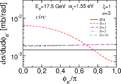
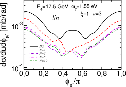
Figure 4: Invariant double-differential cross sections $d^{2}\sigma^{(i)}/du\,d\phi_{e^{\prime}}|_{u=3}$ for various values of $N$ as given in the legends (colored curves). The monochromatic model, $d^{2}\sigma^{(i)}_{IPA}/du\,d\phi_{e^{\prime}}$, is depicted by solid black curves. Left panel: circular polarization, right panel: linear polarization, both for $\xi=1$.

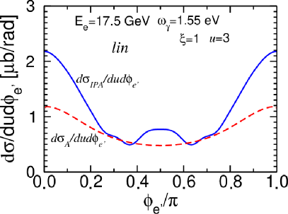
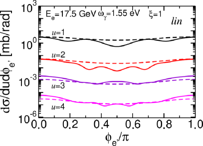
Figure 5: Left panel: Invariant differential cross sections $d^{2}\sigma^{(lin)}_{IPA}/du\,d\phi_{e^{\prime}}|_{u=3}$ according to Eq. (15) (solid curve, as in Fig. 4, here however in a linear scale) and $d^{2}\sigma^{(lin)}_{IPA,large-\xi}/du\,d\phi_{e^{\prime}}|_{u=3}$ according to Eq. (23) (dashed curve) for $\xi=1$. Right panel: The same as in the left panel but for $u=1$, 2, 3 and 4 in $\log$ scale with the same line style. For linear polarization and $\xi=1$.

The fine structures in the angular distribution vanish when turning from the monochromatic model $d^{2}\sigma^{(lin)}_{IPA}/du\,d\phi_{e^{\prime}}$ to the large-$\xi$ limit, see Fig. 5. In the latter case, the double-differential cross section follows from Eq. (18) on account of $\cos\psi=\frac{\tau}{\xi}\cot\phi_{e^{\prime}}$ Ritus as

$$\frac{d^{2}\sigma^{(lin)}_{IPA,large-\xi}}{du\,d\phi_{e^{\prime}}}=\frac{16\alpha^{2}}{\pi^{2}\,\xi^{2}(k\cdot p)\,\sin^{2}\phi_{e^{\prime}}}\frac{1}{(1+u)^{2}}\int\limits_{-\infty}^{\infty}\frac{d\tau|\tau|}{\sin\psi}$$

$$\times\left(\frac{u}{2\chi\sin\psi}\right)^{\frac{1}{3}}[-\Phi^{2}(y)+\left(\frac{2\chi\sin\psi}{u}\right)^{\frac{2}{3}}\left(1+\frac{u^{2}}{2(1+u)}\right)(y\Phi^{2}(y)+{\Phi^{\prime}}^{2}(y))]$$ (23)

with $y=(1+\tau^{2})\left(\frac{u}{2\chi\sin\psi}\right)^{2/3}$.

Note that, in a strict head-on collision, $\phi_{\vec{k}^{\prime}}=\pi+\phi_{e^{\prime}}$, i.e. the azimuthal distribution $d^{2}\sigma/du\,d\phi_{e^{\prime}}$ refers directly to the azimuthal photon distribution $d^{2}\sigma/du\,d\phi_{\vec{k}^{\prime}}$.

To summarize this part we conclude that in the IPA case the dependence of cross sections on the azimuthal angle of outgoing particles appears only for a linearly polarized laser beam. In the case of finite pulse duration, this dependence appears both for circular and linear polarizations, but becomes manifest more clearly for linearly polarized pulses.

IV q-deformed exponential

While for $\xi\approx 1$ the above spectra $d\sigma^{(i)}/du$ and $d\sigma^{(i)}_{IPA}/du$ are near to purely exponential shapes, e.g. for $u>1$, with increasing values of $\xi$ they become more convex, i.e. q-exponentially deformed. Accordingly, we parameterize them by the ansatz

$$\frac{d\sigma_{q}}{du}=\hat{\cal N}\exp_{q}\left(-\frac{u}{x_{0}}\right)$$ (24)

in the interval $u\in[0.5,4]$ with free normalization $\hat{\cal N}$. The q-exponential is defined by $\hat{f}(q,z)\equiv\exp_{q}(z)=[1+(1-q)z]^{\frac{1}{1-q}}$; it obeys $\lim_{q\to 1}\exp_{q}(z)=\exp(z)$. The meaning of the parameters is that of the slope at the origin, $(\partial_{u}\hat{f}/\hat{f})|_{u=0}=-1/x_{0}$, and the normalized curvature $(\hat{f}\partial^{2}_{u}\hat{f})/(\partial_{u}\hat{f})^{2}=q$. The series expansion $\exp_{q}(-u/x_{0})=\exp(-u/x_{0})\left[1-\frac{1}{2}(q-1)(u/x_{0})^{2}+\frac{1}{24}(q-1)^{2}u^{3}(3u-8)/x_{0}^{4}+\cdots+(q-1)^{i}(\cdots)+\cdots\right]$ demonstrates the relation to a purely exponential function, and another series expansion, $\exp_{q}(-u/x_{0})=1-(u/x_{0})+\frac{1}{2}q(u/x_{0})^{2}+\frac{1}{6}q(1-2q)(u/x_{0})^{3}+\cdots$, also helps our understanding of the role of the parameters $x_{0}$ and $q$. In particular, $q=1$ means that a graph of $\log f$ vs. $u$ displays a straight line.

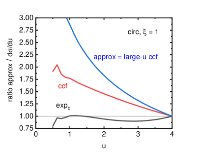
Figure 6: Ratios of the q-exponential fit, Eq. (24), to $d\sigma^{(circ)}_{IPA}/du$ of Eq. (15) are exhibited by black curves with label “$\exp_{q}$” for $\xi=1$ (left panel) and $\xi=10$ (right panel). For illustrative purposes, the chosen normalization $\widehat{\cal N}$ is here such to achieve unity at $u=4$. Analog normalizations are employed for the approximations Eq. (21) (red curves with label “ccf” for $(d\sigma_{ccf}/du)/(d\sigma^{(circ)}_{IPA}/du))$ and Eq. (22) (blue curves with label “approx = large-$u$ ccf” for $(d\sigma_{ccf,large-u}/du)/(d\sigma^{(circ)}_{IPA}/du))$ ). For circular polarization.

The fits of $d\sigma_{q}/du$ describe the original spectra $d\sigma^{(circ)}/du$ with mean deviations typically less than 10% and maximum local deviations of less than $\pm 20$%, despite the many orders of magnitude change of $d\sigma/du$ in the considered interval of $u$. (For $\xi=1$ the differential cross sections run over six orders of magnitude in the displayed range of $u$.) To quantify this we exhibit in Fig. 6 by black curves the ratios $(d\sigma_{q}/du)/(d\sigma^{(circ)}_{IPA}/du)$ by artificially modifying the normalization $\hat{\cal N}\to\widehat{\cal N}$ such to get $\widehat{\cal N}\exp_{q}(-u/x_{0})=d\sigma_{IPA}^{(circ)}/du$ at $u=4$. Obviously, $\widehat{\cal N}$ is not the optimum normalization since only the sub-set $\{x_{0},q\}$ is varied at fixed $\widehat{\cal N}$. The optimum normalization is achieved under unconstrained variation of $\{\hat{\cal N},x_{0},q\}$; it up-shifts the black curves somewhat. For large values of $\xi$, the constant cross field approximation (Eq. (22) (red curves)) describes the results of Eq. (15) even better than the q-exponential, see right panel of Fig. 6, which, however, is superior at smaller values of $\xi$, as recognizable in the left panel. The large-$u$ approximation of the constant cross field approximation Eq. (22) (blue curves) turns out to be less accurate within the considered ranges of $u$ and $\xi$. Nevertheless, given the huge variation of the differential cross section, in particular for smaller values of $\xi$, Eq. (22) provides a useful approximation, as pointed out above.

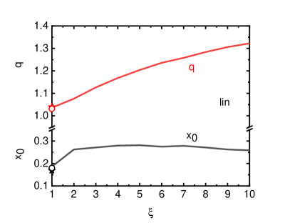
Figure 7: Fits of the cross sections $d\sigma^{(i)}_{IPA}/du$ exhibited in Fig. 2 by the q-exponential Eq. (24) with parameters $x_{0}$ (solid black) and $q$ (solid red) and normalization $\hat{\cal N}$ (not displayed). The fit range is $u\in[\hat{u}_{1},\hat{u}_{1}]$ with $\hat{u}_{1}=0.5$ and $\hat{u}_{2}=4$. (This fit range uncovers the scaled $out$-photon frequencies $\omega^{\prime}/E_{e^{-}}=u/(1+u)\in[0.33\cdots 0.8]$ for on-axis back-scattering. We mention some weak dependence of $x_{0}$ and $q$ and $\hat{\cal N}$ on the fit range parameters $\hat{u}_{1,2}$.) The dashed (dotted) curves in the left panel depict the parameters $x_{0}$ and $q$ when using Eq. (21) ((22)) with $\chi=0.2078\,\xi$ as input. The circles (asterisks) are for fits of the pulse model, $d\sigma^{(i)}/du$ displayed in Fig. 1, for $N=1$ ($N=10$). Left panel: circular polarization, right panel: linear polarization.

Coming back to the parameters of the q-exponential fits, the resulting dependence of $x_{0}$ and $q$ on $\xi$ is displayed in Fig. 7 for $d\sigma^{(i)}_{IPA}/du$ as input. Interestingly, the values of $x_{0}$ stay in between 0.2 and 0.35, with a maximum at $\xi\approx 3$ for circular polarization, while for linear polarization, $x_{0}$ is confined to $x_{0}\in[0.16,0.30]$.

The parameter $q$ increases steadily from 1.02 at $\xi=1$ reaching nearly 1.4 for $\xi=10$. Using $d\sigma^{(i)}/du$ as input (see Fig. 1), one gets the results displayed as circles ($N=1$) and asterisks ($N=10$). These values do not differ noticeably from the ones obtained for the $d\sigma^{(i)}_{IPA}/du$ input. We emphasize that such fits are in the spirit of characterizing data, which run over many orders of magnitude, by a few concise parameters. This is common practice, e.g. in particle and relativistic heavy-ion physics (see remarks in subsection V.2 below).

Using the approximation Eq. (21) as input for the q-exponential fits facilitates the dashed curves in the left panel of Fig. 7, which are near to the solid curves. The large-$u$ approximation of the constant cross field approximation, Eq. (22), as input causes larger differences (dotted curves), in particular for $x_{0}(\xi)$. Nevertheless, a relation emerges between $x_{0}(\chi=\xi k\cdot p/m^{2}=\xi\,0.2078)$ and the famous exponent argument $-2u/3\chi$ in Eq. (22) at $\xi=1$, see the following sub-section.

V Discussion

V.1 Relation to integrated $u$-differential cross sections

Defining the integrated cross section by $\sigma_{c}=\int_{c}^{\infty}du\frac{d\sigma}{du}$, with $\sigma=\sigma_{c}(c\to 0)$ as total cross section, refers to the “cross section with cut-off $c$” considered in HernandezAcosta:2020agu for $\xi={\cal O}(1)$. Since $\int dz\exp_{q}(z)=\exp_{q}(z)(1+(1-q)z)/(2-q)+const$ one gets for the integrated cross section $\sigma_{c}=\hat{\cal N}\exp(-c/x_{0})(1-(1-q)c/x_{0})/(2-q)$, when the description (24) would apply for all values $u\geq c$. This implies $\sigma_{c}\approx\hat{\cal N}\exp(-c/x_{0})$ in leading order at $q\approx 1$, thus recovering the observation in HernandezAcosta:2020agu that the partially integrated cross section displays an exponential dependence on $1/x_{0}$ with $x_{0}\approx 3\chi/2$ at $\xi\approx 1$. We recall the relations $\chi=\xi k\cdot p/m^{2}$ and $\xi=(m/\omega)({\cal E}/{\cal E}_{crit)}$ from (1, 2), thus $\chi=({\cal E}/{\cal E}_{crit})(E_{e^{-}}/m+\sqrt{E_{e^{-}}^{2}/m^{2}-1})$. At the origin of the resulting Schwinger type dependence $\propto\exp\left(-\frac{{\cal E}_{crit}}{{\cal E}}\frac{u}{E_{e^{-}}/m+\sqrt{E_{e^{-}}^{2}/m^{2}-1}}\right)$ is the near-exponential shape of the differential cross section $d\sigma/du$ of the hard-photon tails of the non-linear Compton process. The exponential $1/\chi$-dependence of the differential one-photon Compton cross section has been emphasized also in Dinu:2018efz .

V.2 Thermalized systems

Thermalized systems, e.g. a quark-gluon plasma, with spatial extensions smaller than the photon’s mean-free path, exhibit a photon emission rate $\propto T^{2}\exp\{-E_{\gamma}/T\}\log(\tilde{\alpha}E_{\gamma}/T)$, cf. McLerran:2015mda (here, $T$ stands for the system’s temperature, $E_{\gamma}$ is the photon energy and $\tilde{\alpha}$ denotes a system-specific parameter). The exponential behavior reflects the thermal Boltzmann-Gibbs distribution functions of the constituents, modified by quantum statistics. Otherwise, the particle transverse-momentum spectra observed in ultra-relativistic heavy-ion collisions over nine orders of magnitude, e.g. at the LHC (cf.  figure 1 in Balek:2017man and figures 4 and 5 in Acharya:2018orn for examples among many others), maybe conveniently parameterized either by Boltzmann-Gibbs distributions with one slope parameter (the “temperature”) – modified by a collective flow (resulting in Jüttner functions and thus modifying the exponential shapes) – or by Tsallis distributions Tsallis:1987eu , similar to Eq. (24), which refer to non-extensive thermodynamics and statistics, see Rath:2019cpe .

Having these considerations in mind together with the Schwinger type behavior, one could be tempted to consider the hard-photon emission by an electron traversing a strong background field also as a statistical process of shaking photons off the field-modified vacuum by the disturbance by the electron. The fluctuation in the related “temperature” is directly linked to the non-extensive parameter $q$ and tells us about the departure of the system from an equilibrium state.

V.3 Photon-energy differential cross section

Previous speculations ignore the distinction of the energy/momentum variables and the dimensionless variable $u$. In our case, the energy of the emitted photon, $\omega^{\prime}=\nu^{\prime}m$, and the polar angle $\Theta^{\prime}$ determine the quantity $u=\frac{e^{-\zeta}\nu^{\prime}(1-\cos\Theta^{\prime})}{1-e^{-\zeta}\nu^{\prime}(1-\cos\Theta^{\prime})}$, where the electron energy in lab. determines the rapidity $\zeta$ via $E_{e^{-}}=m\cosh\zeta$. Using the energy-momentum balance in the form $u(\nu^{\prime},n)=(n\nu-\nu^{\prime})/(\kappa_{n}-n\nu+\nu^{\prime})$ with $\kappa_{n}=n\nu-\frac{1}{2}e^{\zeta}+\frac{1}{2}(1+\xi^{2})e^{-\zeta}$ Harvey:2009ry eliminates the scattering angle in favor of the harmonic number $n$. Casting the differential cross section (15) in the form $d\sigma/du=\sum_{n=1}^{\infty}d\sigma_{n}/du$ one arrives at $d\sigma_{n}/du=-(d\sigma_{n}/d\nu^{\prime})\,\kappa_{n}/(1+u(\nu^{\prime},n))^{2}$. For the given kinematics one can show that in leading order the relation

$$\frac{d\sigma_{n}}{du}=\frac{|q_{z}-n\omega|}{(1+u)^{2}}\frac{d\sigma_{n}}{d\omega^{\prime}}\approx\frac{|\kappa_{\hat{n}}|}{(1+u(\nu^{\prime},\hat{n}))^{2}}\,\frac{d\sigma_{n}}{d\nu^{\prime}}$$ (25)

follows for the partial cross sections, where $q_{z}=p_{z}-\xi^{3}\omega/(2\chi)k_{z}$, $p_{z}=\sqrt{E_{e^{-}}^{2}-m^{2}}$ and $k_{z}=\omega$. This relation also holds for pulses by replacing $n\to\ell$ and $q_{z}\to p_{z}$. Numerically, we find that any $n\to\hat{n}\ll 10^{7}$ is useful. The key for the simple relations of $d\sigma/du$, $d\sigma/d\omega^{\prime}$ and $d\sigma/d\nu^{\prime}$ is $e^{\zeta}\gg 1$ and $\nu=\omega/m\ll 1$. The mapping $\omega^{\prime}\mapsto u$ changes the concave curves $d\sigma/d\omega^{\prime}$ as a function of $\omega^{\prime}$ into convex curves $d\sigma/du$ as a function of $u$. The range $u\geq 1$ is beyond the pronounced harmonic structures – it corresponds to $\omega^{\prime}>8.5$ GeV, where local structures can be considered as sub-leading modulations of the gross shape, in particular for linear polarization. To highlight these relations we exhibit in Fig. 8 the differential cross sections $d\sigma/d\omega^{\prime}$ as a function of $\omega^{\prime}$. One observes a fast decrease of the cross sections at $\omega^{\prime}>11$ GeV and weak dependence on the pulse duration for $N>1$, similar to that as for $d\sigma/du$ discussed above in the context of the bottom panels in Fig. 1. Note that we consider here only the case of $\xi=1$. At lower field intensities, e.g. $\xi=0.1$, the cross sections would display pronounced harmonic structures analog to that of $d\sigma/du$, exhibited in the top row of Fig. 1.

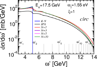
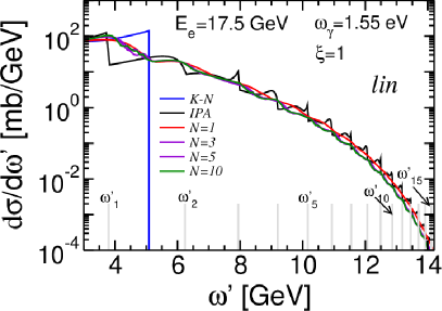
Figure 8: Differential cross sections $d\sigma^{(i)}/d\omega^{\prime}$ for $\xi=1$ analog to bottom row in Fig. 1. The harmonic thresholds $\omega_{n}^{\prime}$ follow from inverting the above quoted equation of $u(\nu^{\prime}=\omega^{\prime}/m,n)$ from energy-momentum balance.

VI summary

In summary we point out that the non-linear Compton process, i.e. the one-photon emission by an electron moving with tens GeV energy through an optical laser pulse of moderate intensity $\xi\gtrsim 1$, gives rise to q-deformed exponential photon tails: $d\sigma/du\propto\exp_{q}(-u/x_{0})$, where $u=k\cdot k^{\prime}/(p\cdot p-k\cdot k^{\prime})$ is the dimensionless Ritus variable meaning the light-cone momentum-transfer from the $in$-electron to the $out$-photon, which is, for envisaged kinematics at LUXE and E-320, closely related to the photon energy $\omega^{\prime}$. For $\xi\approx 1$, the slope parameter $x_{0}$ is in the order of $\chi$, that is another Ritus variable, which measures the (electric) field strength in the electron’s rest system, explicitly $\chi=({\cal E}/{\cal E}_{crit})(E_{e^{-}}/m+\sqrt{(E_{e^{-}}/m{\color[rgb]{0,0,0})}^{2}-1})$. We emphasize the Schwinger type dependence with the enhancement factor $E_{e^{-}}/m+\sqrt{(E_{e^{-}}/m{\color[rgb]{0,0,0})}^{2}-1}$ which reduces the exponential suppression, analog to the dynamically assisted Schwinger process with momentum space information Orthaber:2011cm . The (near-) exponential differential cross section results in a (near-) exponential integrated cross section when considering only the high-energy tail HernandezAcosta:2020agu , again with Schwinger type dependence.

The high-energy photon tails with $\omega^{\prime}>1$ GeV are accessible by detectors in development Fleck:2020opg , e.g. for the LUXE set up Abramowicz:2019gvx ; Abramowicz:2021zja . The present paper tests the robustness of previous results HernandezAcosta:2020agu based on the monochromatic laser beam model with circular polarization. Focusing on the region of $\xi\gtrsim 1$ we consider the effects of laser polarizations and laser pulse shapes and durations as well. We find some support of the monochromatic model even for short pulses when considering the differential spectra $d\sigma/du$. The difference of circular and linear laser polarizations shows up most clearly in azimuthal $out$-electron distributions, while the gross features of the differential cross sections $d\sigma/du$ or $d\sigma/d\omega^{\prime}$ and the q-exponential parameters and their dependence on the laser intensity $\xi\gtrsim 1$ as well are fairly similar. Only in the limit of a monochromatic laser beam and not too large intensities, harmonic structures modulate noticeably the differential spectra. The presented numerical evaluations of the essentially known formalism may serve as benchmark for more refined approaches. These should account for ponderomotive broadening effects, beam profile simulations (cf. figure 6 and section V.B in Heinzl:2009nd for estimates of such effects) and genuine multiple-photon emissions Dinu:2018efz ; Blackburn:2018sfn ; Dinu:2019pau beyond the nonlinear two-photon Compton process Lotstedt:2009zz ; Loetstedt:2009zzz ; Seipt:2012tn ; Mackenroth:2012rb . The q-exponential parameterization of spectra can provide a useful interpolation tool thereby.

Finally, we emphasize the multi-photon (up to non-perturbative) effects which shape the photon tails, thus probing the non-linear regime of QED. As another avenue towards further developments we mention, e.g., extensions of the standard model of particle physics by novel degrees of freedom, represented by dark photons or axions which may affect the electromagnetic sector and show up as modifications of the here investigated photon spectra and seeded subsequent processes.