A Krylov-Schur like method for computing the best rank-$(r_{1},r_{2},r_{3})$ approximation of large and sparse tensors

Abstract

The paper is concerned with methods for computing the best low multilinear rank approximation of large and sparse tensors. Krylov-type methods have been used for this problem; here block versions are introduced. For the computation of partial eigenvalue and singular value decompositions of matrices the Krylov-Schur (restarted Arnoldi) method is used. We describe a generalization of this method to tensors, for computing the best low multilinear rank approximation of large and sparse tensors. In analogy to the matrix case, the large tensor is only accessed in multiplications between the tensor and blocks of vectors, thus avoiding excessive memory usage. It is proved that, if the starting approximation is good enough, then the tensor Krylov-Schur method is convergent. Numerical examples are given for synthetic tensors and sparse tensors from applications, which demonstrate that for most large problems the Krylov-Schur method converges faster and more robustly than higher order orthogonal iteration.

65F99, 15A69, 65F15.

1 Introduction

In many applications of today, large and sparse data sets are generated that are organized in more than two categories. Such multi-mode data can be represented by tensors. They arise in applications of data sciences, such as web link analysis, cross-language information retrieval and social network analysis, see, e.g., [31] and the survey [30]. The effective analysis of tensor data requires the development of methods that can identify the inherent relations that exist in the data, and that scale to large data sets. Low rank approximation is one such method, and much research has been done in recent years in this area; a few examples that are related to the work of this paper are given in [2, 6, 9, 14, 23, 28, 35, 40, 41, 50]. However, most of these methods are intended for small to medium size tensors. The objective of this paper is to develop an algorithm for low-rank approximation of large and sparse tensors.

We consider the problem of approximating a 3-mode tensor $\mathcal{A}$ by another tensor $\mathcal{B}$,

(1) $$\min\limits_{\mathcal{B}}\|\mathcal{A}-\mathcal{B}\|,$$

where the norm is the Frobenius norm, and $\mathcal{B}$ has low multilinear rank-$(r_{1},r_{2},r_{3})$ (for definitions of the concepts used in this introduction, see Section 2). We will assume that $\mathcal{A}$ is large and sparse. This problem can be written

(2) $$\min_{\mathcal{F},U,V,W}\|\mathcal{A}-\bm{\left(}U,V,W\bm{}\bm{\cdot}\mathcal{F}\|,\quad\mathrm{subject~{}to}\quad U^{T}U=I_{r_{1}},\quad V^{T}V=I_{r_{2}},\quad W^{T}W=I_{r_{3}},$$

where $\mathcal{F}\in\mathbb{R}^{r_{1}\times r_{2}\times r_{3}}$ is a tensor of small dimensions, and $\bm{\left(}U,V,W\bm{}\bm{\cdot}\mathcal{F}$ denotes matrix-tensor multiplication in all three modes. This is the best rank-$(r_{1},r_{2},r_{3})$ approximation problem [9], and it is a special case of Tucker tensor approximation [47, 48]. It can be considered as a generalization of the problem of computing the Singular Value Decomposition (SVD) of a matrix [15]. In fact, a partial SVD solves the matrix approximation problem corresponding to (1), see e.g. [20, Chapter 2.4].

In this paper we develop a Block Krylov-Schur like (BKS) method for computing the best rank-$(r_{1},r_{2},r_{3})$ approximation of large and sparse tensors which are symmetric with respect to two modes. We are specially interested in small values of the rank, as in the two parallel papers [17, 16], where it is essential to use the best approximation rather than any Tucker approximation.

Krylov methods are routinely used to compute partial SVD’s (and eigenvalue decompositions) of large sparse matrices [32]. In [40] we introduced a generalization of Krylov methods to tensors. It was shown experimentally that tensor Krylov-type methods have similar approximation properties as the corresponding matrix Krylov methods. In this paper we present block versions of Krylov-type methods for tensors, which are expected to be more efficient than the methods in [40]. Having problems in mind, where the tensor is symmetric with respect to two modes (e.g. sequences of adjacency matrices of graphs), we formulate the block methods in terms of such tensors.

Even if matrix Krylov methods give low rank approximations, their convergence properties are usually not good enough, and, if used straightforwardly, they may require excessive memory and computer time. Therefore they are accelerated using restart techniques [32], which are equivalent to the Krylov-Schur method [44]. We here present a tensor Krylov-Schur like method, and show that it can be used to compute best multilinear low-rank approximations of large and sparse tensors.

The Krylov-Schur method is an inner-outer iteration. In the outer iteration we start from an approximate solution and generate new blocks of orthogonal vectors, using Krylov-type block methods. Thus we use the large tensor only in tensor-matrix multiplications, where the matrix has few columns (this is analogous to the use of block Krylov methods for large matrices). Then we project the problem (2) to a smaller problem of the same type, which we solve in the inner iterations, using a method for problems with a medium-size, dense tensor. The problem can be formulated as one on a product of Grassmann manifolds [14]. In our experiments we use a Newton-Grassmann method. As a stopping criterion for the outer iteration we use the norm of the Grassmann gradient of the objective function. We show that this gradient can be computed efficiently in terms of the small projected problem.

We also prove that, if the starting approximation the Krylov-Schur method is good enough, the BKS method is convergent.

The literature on algorithms for best rank-$(r_{1},r_{2},r_{3})$ approximation of large and sparse tensors is not extensive [29, 21, 26]. To the best of our knowledge the present paper is the first one that goes significantly beyond the Higher Order Orthogonal Iteration (HOOI) [9]. Our experiments indicate that the new method is more efficient and robust than HOOI for large and sparse tensors.

The paper is organized as follows. Some tensor concepts are introduced in Section 2. The Krylov-Schur procedure for matrices is sketched in Section 3. In Section 4 block Krylov-type methods for tensors are described. The tensor Krylov-Schur method is presented and analyzed in Section 5. Some numerical examples are given in Section 6 that illustrate the accuracy and efficiency of the Krylov-Schur method. In particular, we demonstrate that for less well-conditioned approximation problems, the new method converges faster than HOOI [9]. We are especially interested in tensors that are symmetric with respect to the first two modes (e.g. tensor consisting of a sequence of adjacency matrices of undirected graphs). Therefore the block Krylov-type methods and the numerical examples are given in terms of such tensors.

The method presented in this paper is “like” a Krylov-Schur method for two reasons. The tensor Krylov-type method is not a Krylov method in a strict sense, as it does not build bases for Krylov subspaces [40]. The method is not a real Krylov-Schur method as it does not build and manipulate a Hessenberg matrix; instead it uses a tensor, which is in some ways similar to Hessenberg. However, this structure is not utilized. For ease of presentation we will sometimes omit “like” and “type”.

2 Tensor concepts and preliminaries

2.1 Notation

Throughout this paper we use of the following notations. Vectors will be denoted by lower case roman letters, e.g., $a$ and $b$, matrices by capital roman letters, e.g., $A$ and $B$ and tensors by calligraphic letters, e.g., ${\mathcal{A}}$ and ${\mathcal{B}}$.

Notice that sometimes we will not explicitly mention the dimensions of matrices and tensors, and assume that they are such that the operations are well-defined. Also, for simplicity of notation and presentation, we will restricted ourselves to tensors of order 3, which are defined in the next paragraph. The generalization to higher order tensors is straightforward. For more general definitions we refer reader to [3].

A tensor will be viewed as a multidimensional array of real numbers. The order of a tensor is the number of dimensions, also known as modes, e.g., a 3-dimensional array, $\mathcal{A}\in\mathbb{R}^{l\times m\times n}$, is called a tensor of order 3 or 3-tensor. A fiber is a one-dimensional section of a tensor, obtained by fixing all indices except one; $\mathcal{A}(i,:,k)$ is referred to as a mode-2 fiber. A slice is a two-dimensional section of a tensor, obtained by fixing one index; $\mathcal{A}(i,:,:)$ is a mode-1 slice or 1-slice. A particular element of a 3-tensor $\mathcal{A}$ can be denoted in two different way, i.e., ”matlab-like” notation and standard subscripts with $\mathcal{A}(i,j,k)$ and $a_{ijk}$, respectively.

Definition 2.1.

A 3-tensor $\mathcal{A}\in\mathbb{R}^{m\times m\times n}$ is called (1,2)-symmetric if all its 3-slices are symmetric, i.e.,

$$\mathcal{A}(i,j,k)=\mathcal{A}(j,i,k),\qquad i,j=1,2,\ldots,m,\qquad k=1,2,\ldots,n.$$

Symmetry with respect to any two modes and for tensors of higher order than 3 can be defined analogously.

We use $I_{k}$ for the identity matrix of dimension $k$.

2.2 Multilinear tensor-matrix multiplication

We first consider the multiplication of a tensor by a matrix. When a tensor is multiplied by a single matrix in mode i, say, we will call the operation the mode-i multilinear multiplication (or mode-i product) of a tensor by a matrix. For example the mode-1 product of a tensor $\mathcal{A}\in\mathbb{R}^{l\times m\times n}$ by a matrix $U\in\mathbb{R}^{p\times l}$ is defined

$$\mathbb{R}^{p\times m\times n}\ni\mathcal{B}=\bm{\left(}U\bm{}_{1}\bm{\cdot}\mathcal{A},\qquad b_{ijk}=\sum_{\alpha=1}^{l}u_{i\alpha}a_{\alpha jk}.$$

This means that all mode-1 fibers in the 3-tensor $\mathcal{A}$ are multiplied by the matrix $U$. The mode-2 and the mode-3 product are defined in a similar way. Let the matrices $V\in\mathbb{R}^{q\times m}$ and $W\in\mathbb{R}^{r\times n}$; multiplication along all three modes is defined

$$\mathbb{R}^{p\times q\times r}\ni\mathcal{B}=\bm{\left(}U,V,W\bm{}\bm{\cdot}\mathcal{A},\qquad b_{ijk}=\sum_{\alpha=1}^{l}\sum_{\beta=1}^{m}\sum_{\gamma=1}^{n}u_{i\alpha}v_{j\beta}w_{k\gamma}a_{\alpha\beta\gamma}.$$

For multiplication with a transposed matrix $X\in\mathbb{R}^{l\times s}$ it is convenient to introduce a separate notation,

$$\mathbb{R}^{s\times m\times n}\ni\mathcal{B}=\bm{\left(}X^{T}\bm{}_{1}\bm{\cdot}\mathcal{A}=\mathcal{A}\bm{\cdot}\bm{\left(}X\bm{}_{1},\qquad b_{i,j,k}=\sum_{\alpha=1}^{l}x_{\alpha i}a_{\alpha jk}.$$

In a similar way if $x\in\mathbb{R}^{l}$ then

$$\mathbb{R}^{1\times m\times n}\ni\mathcal{B}=\bm{\left(}x^{T}\bm{}_{1}\bm{\cdot}\mathcal{A}=\mathcal{A}\bm{\cdot}\bm{\left(}x\bm{}_{1}=B\in\mathbb{R}^{m\times n}.$$

Thus the tensor $\mathcal{B}$ is identified with a matrix $B$.

2.3 Inner product and norm, contractions

The inner product of two tensors $\mathcal{A}$ and $\mathcal{B}$ of the same order and dimensions is denoted by $\langle\mathcal{A},\mathcal{B}\rangle$ and is computed as a sum of element-wise products over all the indices, that is

$$\langle\mathcal{A},\mathcal{B}\rangle=\sum_{i,j,k}a_{ijk}b_{ijk}$$

The product allows us to define the Frobenius norm of a tensor $\mathcal{A}$ as

$$\|\mathcal{A}\|=\langle\mathcal{A},\mathcal{A}\rangle^{1/2}.$$

As in the matrix case the Frobenius norm of a tensor is invariant under orthogonal transformations, i.e., $\|A\|=\|\bm{\left(}U,V,W\bm{}\bm{\cdot}\mathcal{A}\|$, for orthogonal matrices $U$, $V$, and $W$. This follows immediately from the fact that mode-i multiplication by an orthogonal matrix does not change the Euclidean length of the mode-i fibers.

The inner product is a contraction. We also define partial contractions that involve less than three modes,

$$\mathcal{C} =\langle\mathcal{A},\mathcal{B}\rangle_{1}, c_{jk\mu\nu} =\sum_{\lambda}a_{\lambda jk}b_{\lambda\mu\nu},$$

$$\mathcal{D} =\langle\mathcal{A},\mathcal{B}\rangle_{1,2}, d_{k\nu} =\sum_{\lambda,\mu}a_{\lambda\mu k}b_{\lambda\mu\nu}.$$

We use negative subscripts to denote partial contractions in all but one mode,

(3) $$\langle\mathcal{A},\mathcal{B}\rangle_{-1}=\langle\mathcal{A},\mathcal{B}\rangle_{2,3}.$$

The result is a matrix (order 2 tensor) of inner products between the mode-1 slices of the two tensors. For partial contractions only the contracted modes are required to be equal, so the result matrix may be rectangular.

2.4 Multilinear rank

Unlike the matrix case, there is no unique definition of the rank of a tensor. In this paper we consider the concept of multilinear rank defined by Hitchcock [22]. Let $A^{(i)}$ denote the mode-$i$ unfolding (matricization) of $\mathcal{A}$ (using some ordering of the vectors),

$$A^{(i)}=\mathtt{unfold}_{i}(\mathcal{A}),$$

where the columns of $A^{(i)}$ are all mode-$i$ fibers [8]. Similarly, let $\mathtt{fold}_{i}$ be the inverse of $\mathtt{unfold}_{i}$. The multilinear rank of a third order tensor $\mathcal{A}$ is an integer triplet $(p,q,r)$ such that

$$p=\mathrm{rank}(A^{(1)}),\qquad q=\mathrm{rank}(A^{(2)}),\qquad r=\mathrm{rank}(A^{(3)}),$$

where $\mathrm{rank}(A^{(i)})$ is the matrix rank. In this paper we will deal only with multilinear rank, and we will use the notation rank-$(p,q,r)$, and $\mathrm{rank}(A)=(p,q,r)$. For matrices the rank is obtained via the svd; see, e.g., [20, Chapter 2]. In exact arithmetic the multilinear rank can be computed using the higher order singular value decomposition (HOSVD) [8].

2.5 Best rank-$(r_{1},r_{2},r_{3})$ approximation

The problem (1) of approximating a given tensor $\mathcal{A}\in\mathbb{R}^{l\times m\times n}$ by another tensor $\mathcal{B}$ of equal dimensions but of lower rank, occurs in many modern applications, e.g., machine learning [33], pattern classification [39], analytical and quantum chemistry [42, 27], and signal processing [7]. We assume that $\mathrm{rank}(\mathcal{B})=(r_{1},r_{2},r_{3})$, which means that $\mathcal{B}$ can be written as a product of a core tensor $\mathcal{F}\in\mathbb{R}^{r_{1}\times r_{2}\times r_{3}}$ and three matrices,

$$\mathcal{B}=\bm{\left(}U,V,W\bm{}\bm{\cdot}\mathcal{F},\qquad\mathcal{B}(i,j,k)=\sum_{\lambda,\mu,\nu=1}^{r_{1},r_{2},r_{3}}u_{i\lambda}v_{j\mu}w_{k\nu}f_{\lambda\mu\nu},$$

where $U\in\mathbb{R}^{l\times r_{1}}$, $V\in\mathbb{R}^{m\times r_{2}}$, and $W\in\mathbb{R}^{n\times r_{3}}$ are full column rank matrices. Without loss a generality, we can suppose that $U$, $V$ and $W$ have orthonormal columns, as any nonorthogonality may be incorporated into $\mathcal{F}$. Therefore the best multilinear low rank problem (1) can be written as

(4) $$\min\limits_{\mathcal{F},U,V,W}\|\mathcal{A}-\bm{\left(}U,V,W\bm{}\bm{\cdot}\mathcal{F}\|,\quad\mathrm{subject~{}to}\quad U^{T}U=I_{r_{1}},\quad V^{T}V=I_{r_{2}},\quad W^{T}W=I_{r_{3}}.$$

There are a few major differences between the best low rank approximation of matrices and 3-mode tensors and higher. In the matrix case, the explicit solution of corresponding problem can be obtained from the SVD, see the Eckart-Young property in [20, Theorem 2.4.8]. A simple proof is given in [13, Theorem 6.7]. There is no known closed form solution for the minimization problem (4), but it can be shown that this is a well-defined problem in the sense that for any $(r_{1},r_{2},r_{3})$ a solution exists [10, Corollary 4.5]. Several iterative methods for computing the low rank approximation for small and medium size tensors have been proposed, see [9, 14, 24, 41]. In [9], it is shown that (4) is equivalent to following maximization problem

(5) $$\max\limits_{U,V,W}\Phi(U,V,W),\quad\mathrm{subject~{}to}\quad U^{T}U=I_{r_{1}},\quad V^{T}V=I_{r_{2}},\quad W^{T}W=I_{r_{3}},$$

where $\Phi(U,V,W)=\|\mathcal{A}\bm{\cdot}\bm{\left(}U,V,W\bm{}\|^{2}$. Since the norm is invariant under orthogonal transformations, it holds that $\Phi(U,V,W)=\Phi(UQ_{1},VQ_{2},WQ_{3})$ for any orthogonal matrices $Q_{1}\in\mathbb{R}^{r_{1}\times r_{1}}$, $Q_{2}\in\mathbb{R}^{r_{2}\times r_{2}}$ and $Q_{3}\in\mathbb{R}^{r_{3}\times r_{3}}$. Hence (5) is equivalent to a maximization problem over a product of Grassmann manifold; for optimization on matrix manifolds, see [12, 1, 23, 24].

After computing the optimal $U$, $V$ and $W$ the optimal $\mathcal{F}$ can be obtained by considering the minimization of (4) as a linear least squares problem with unknown $\mathcal{F}$.

Lemma 2.2.

Let $\mathcal{A}\in\mathbb{R}^{l\times\times m\times n}$ be given along with three matrices with orthonormal columns, $U\in\mathbb{R}^{l\times r_{1}}$, $V\in\mathbb{R}^{m\times r_{2}}$, and $W\in\mathbb{R}^{n\times r_{3}}$, where $r_{1}\leq l$, $r_{2}\leq m$, and $r_{3}\leq n$. Then the least squares problem

$$\min\limits_{\mathcal{F}}\|\mathcal{A}-\bm{\left(}U,V,W\bm{}\bm{\cdot}\mathcal{F}\|$$

has the unique solution

(6) $$\mathcal{F}=\bm{\left(}U^{T},V^{T},W^{T}\bm{}\bm{\cdot}\mathcal{A}=\mathcal{A}\bm{\cdot}\bm{\left(}U,V,W\bm{}.$$

For a proof, see e.g. [9, 40]. The tensor $\mathcal{F}$ is a generalization of the matrix Rayleigh quotient.

2.6 Gradient on the product manifold

In [14] a Newton-Grassmann method is derived for computing the solution of maximization problem (5). The constraints on the unknown matrices $U$, $V$, and $W$ are taken into account by formulating the problem as an optimization problem on a product of three Grassmann manifolds. In this paper we will need the gradient of $\Phi$ in the tangent space of the product manifold for a stopping criterion. This gradient can be expressed in the ambient coordinate system, or in local coordinates. In the context of the new methods presented it is practical and more efficient to use local coordinate representations, see Proposition 4.3. Let $(U\,U_{\perp})$ denote the enlargement of $U$ to a square orthogonal matrix, and use the analogous notation for $V$ and $W$. Then the Grassmann gradient at $(U,V,W)$ can be written as

$$\nabla_{\mathrm{local}}(U,V,W)=(\langle\mathcal{F}^{1}_{\perp},\mathcal{F}\rangle_{-1},\langle\mathcal{F}^{2}_{\perp},\mathcal{F}\rangle_{-2},\langle\mathcal{F}^{3}_{\perp},\mathcal{F}\rangle_{-3}),$$

where $\mathcal{F}^{1}_{\perp}=\mathcal{A}\bm{\cdot}\bm{\left(}U_{\perp},V,W\bm{}$, $\mathcal{F}^{2}_{\perp}=\mathcal{A}\bm{\cdot}\bm{\left(}U,V_{\perp},W\bm{}$, and $\mathcal{F}^{3}_{\perp}=\mathcal{A}\bm{\cdot}\bm{\left(}U,V,W_{\perp}\bm{}$. In the context of the HOOI, see Section 6.1, it is more efficient to use global coordinates. For instance, the first component of the gradient can be computed as

$$(I-UU^{\sf T})\Gamma_{1}=\Gamma_{1}-U(U^{\sf T}\Gamma_{1}),\qquad\Gamma_{1}=\langle\mathcal{A}\bm{\cdot}\bm{\left(}V,W\bm{}_{2,3},\mathcal{F}\rangle_{-1}.$$

For more details on coordinate representations for this problem, see [14], [15, Section 3.2]. In the rest of this paper, the concept G-gradient will mean the Grassmann gradient in global or local coordinates.

2.7 Conditioning of the best approximation problem

The best rank-$r$ approximation problem for a matrix $A$ is not unique if the singular values satisfy $\sigma_{r}(A)=\sigma_{r+1}(A)$. The problem is ill-conditioned if the gap is small, i.e. $\sigma_{r}(A)>\sigma_{r+1}(A)$ but $\sigma_{r}(A)\approx\sigma_{r+1}(A)$, see e.g. [45, Chapter 3], [20, Chapter 8.6]. A similar situation exists for the tensor case [15, Corollary 4.5] (note that the perturbation theory for the SVD is a special case of that for the best rank-$(r_{1},r_{2},r_{3})$ approximation of a tensor). Define

$$s_{i}^{(k)} =(\lambda_{i}(\langle\mathcal{F},\mathcal{F}\rangle_{-k}))^{1/2},\qquad i=1,2,\ldots,r_{k},\quad k=1,2,3,$$

$$s_{r_{k}+1}^{(k)} =(\lambda_{\max}(\langle\mathcal{F}_{\perp}^{k},\mathcal{F}_{\perp}^{k}\rangle_{-k}))^{1/2},\qquad k=1,2,3,$$

where the $\lambda$’s are eigenvalues, in descending order, of the symmetric matrices. We will refer to these quantities as S-values. Then we can define three gaps, one for each mode,

$$\operatorname{gap}_{k}=s_{r_{k}}^{(k)}-s_{r_{k}+1}^{(k)},\qquad k=1,2,3.$$

(In the matrix case, there is only one set of $s_{i}^{(k)}$, which are the singular values). It is shown in [15, Section 5.3] that the gaps can be taken as measures of the conditioning of the best approximation problem. If, for any $k$, $s_{r_{k}}^{(k)}$ is considerably larger than $s_{r_{k}+1}^{(k)}$ then the approximation problem is well-conditioned with respect to mode $k$. Conversely, if the gap is small, then the problem is ill-conditioned.

3 Krylov methods for matrices

Krylov subspace methods are the main class of algorithms for solving iteratively large and sparse matrix problems. Here we give a brief introduction to Krylov methods, illustrating with the Arnoldi method.

For a given square matrix $A\in\mathbb{R}^{n\times n}$ and a nonzero vector $u\in\mathbb{R}^{n}$ the subspace

(7) $$\mathcal{K}_{k}(A,u)=\mathrm{span}\{u,Au,A^{2}u,\ldots,A^{k-1}u\}$$

is called the Krylov subspace of dimension $k$ associated with $A$ and $u$ [20, Chapter 10]. The Arnoldi process [20, Chapter 10] which is obtained by applying Gram-Schmidt orthogonalization, generates an orthogonal basis for the Krylov subspace (7). The recursive Arnoldi process is equivalent to the matrix equation

(8) $$AU_{k}=U_{k+1}\hat{H_{k}},$$

where $U_{k}=[u_{1},\ldots,u_{k}]$ is an orthogonal matrix and $\hat{H_{k}}\in\mathbb{R}^{(k+1)\times k}$ is an Hessenberg matrix with orthogonalization coefficients. Using this factorization one can compute an approximate solution of a linear system or an eigenvalue problem with coefficient matrix $A$ by projecting onto the low dimensional subspace $U_{k}$.

3.1 The Krylov-Schur approach to computing low rank approximations

The Arnoldi and Lanczos methods (see, e.g., [20, Chapter 10], [45, Chapter 5]) are designed for computing the eigenvalues of large and sparse matrices. Writing the Krylov decomposition (8) in the form

(9) $$AU_{k}=U_{k}H_{k}+\beta_{k}u_{k+1}e_{k}^{T},$$

approximations are obtained by computing the eigenvalues of $H_{k}$ (the Ritz values), using an algorithm for dense matrices. A problem with this approach is that when $k$ grows the cost for orthogonalizing a newly generated vector against the columns of $U_{k}$ increases. In addition, since $U_{k}$ is dense, the memory requirements may increase too much. In order to save memory and work, an implicit restarting Arnoldi technique (IRA) was developed [43], and implemented in the highly successful ARPACK package [32]. In [44] Stewart proposed a Krylov-Schur method which is mathematically equivalent to IRA. In the following we give a brief introduction to the Krylov-Schur method, based on [45, Chapter 5].

Consider the Krylov decomposition (9) of $A$, which is obtained after $k$ steps of the Arnoldi recursion. Let $k=r+k_{2}$ where $r$ is the number of $A$’s eigenvalues that we want to compute. The Schur decomposition of $H_{k}$ is

(10) $$H_{k}=QT_{k}Q^{T},$$

where $Q$ and $T_{k}$ are orthogonal and upper triangular matrices, respectively. Partition $T_{k}$ and $Q$ as

(11) $$T_{k}=\begin{pmatrix}T_{11}&T_{12}\\ 0&T_{22}\\ \end{pmatrix},\qquad Q=[Q_{1}\;Q_{2}],$$

where $Q_{1}\in\mathbb{R}^{k\times r}$, $Q_{2}\in\mathbb{R}^{k\times k_{2}}$, and the eigenvalues have been ordered such that those of $T_{11}\in\mathbb{R}^{r\times r}$ are of interest and those of $T_{22}\in\mathbb{R}^{k_{2}\times k_{2}}$ are not. The Krylov decomposition (9) can now be written

(12) $$A(U_{k}Q_{1}\;U_{k}Q_{2})=(U_{k}Q_{1}\;U_{k}Q_{2})\begin{pmatrix}T_{11}&T_{12}\\ 0&T_{22}\\ \end{pmatrix}+u_{k+1}(b_{1,k+1}^{T}\;b_{2,k+1}^{T}),$$

where $(b_{1,k+1}^{T}\;b_{2,k+1}^{T})=(\beta_{k}e_{k}^{T}Q_{1}\;\beta_{k}e_{k}^{T}Q_{2})$. Then

(13) $$A\hat{U}_{r}=\hat{U}_{r}T_{11}+u_{k+1}b_{1,k+1}^{T},$$

where $\hat{U}_{r}=U_{k}Q_{1}$, is also a Krylov decomposition. The main idea of the Krylov-Schur algorithm is to repeatedly expand (13) to dimension $k$, using the Arnoldi recursion, and then reduce it back to dimension $r$. The dimension of $H_{k}$ is assumed to be much smaller than that of $A$, which makes it possible to compute the Schur decomposition of $H_{k}$ using the dense QR algorithm (implemented in LAPACK). A sketch of this method [45, Chapter 5] is given in Algorithm 1.

  Given: matrix $A$, the number of desired eigenvalues $r$ and the number of steps $k$.

  Build a Krylov decomposition (9) of $A$.

  Until convergence

   Compute the Schur decomposition (10) and partition as in (11) with the $r$

    desired eigenvalues in the block $T_{11}$.  

   Discard the unwanted eigenvalues and save the truncated Krylov-Schur

    decomposition (13).  

   Check convergence  

   Expand the Krylov decomposition (13) to one of dimension $k$.

Algorithm 1 The Krylov-Schur algorithm

The convergence check is based on the eigenvalue residual [45, Chapter 5].

4 Krylov-type methods for tensors

Krylov-type methods that generalize the Arnoldi method to tensors are proposed in [40]. The methods are called Krylov-type methods, because the recursions are generalizations of matrix Krylov recursions, but no analogues of Krylov subspaces can be identified (to our knowledge). These methods are also inspired by Golub-Kahan bidiagonalization [19]. The bidiagonalization process generates two sequences of orthonormal basis vectors for certain Krylov subspaces. In the tensor case three sequences of orthogonal basis vectors are generated that are used to compute a core tensor that corresponds to the matrix $H_{k}$ in (9). For matrix Krylov methods, once an initial vector has been selected, the following vectors are determined uniquely; in the tensor case, one can choose different combinations of previously computed basis vectors. So there are different variants of tensor Krylov-type methods. We describe briefly two examples in the following.

4.1 Minimal Krylov recursion

For a given third order tensor $\mathcal{A}\in\mathbb{R}^{l\times m\times n}$ and starting two vectors, $u_{1}\in\mathbb{R}^{l}$ and $v_{1}\in\mathbb{R}^{m}$, we can obtain a third mode vector by $w_{1}=\mathcal{A}\bm{\cdot}\bm{\left(}u_{1},v_{1}\bm{}_{1,2}\in\mathbb{R}^{n}$. By using the most recently obtained vectors, three sequences of vectors can be generated. Using the modified Gram-Schmidt process, a newly generated vector is immediately orthogonalized against all the previous ones in its mode. The minimal Krylov recursion [40, Algorithm 3],which can be seen as a generalization of the Golub-Kahan bidiagonalization method, is given in Algorithm 2. The $\mathtt{orth}$ function orthogonalizes $\hat{u}$ against $U_{i}$, and normalizes it.

  Given: two normalized starting vectors $u_{1}$ and $v_{1}$,

  $\alpha_{w}w_{1}=\mathcal{A}\bm{\cdot}\bm{\left(}u_{1},v_{1}\bm{}_{1,2}$

  for $i=1,2,\ldots,k-1$ do

     $\hat{u}=\mathcal{A}\bm{\cdot}\bm{\left(}v_{i},w_{i}\bm{}_{2,3};\quad u_{i+1}=\mathtt{orth}(\hat{u},U_{i});\quad U_{i+1}=[U_{i}\;u_{i+1}]$

     $\hat{v}=\mathcal{A}\bm{\cdot}\bm{\left(}u_{i+1},w_{i}\bm{}_{1,3};\quad v_{i+1}=\mathtt{orth}(\hat{v},V_{i});\quad V_{i+1}=[V_{i}\;v_{i+1}]$

     $\hat{w}=\mathcal{A}\bm{\cdot}\bm{\left(}u_{i+1},v_{i+1}\bm{}_{1,2};\quad w_{i+1}=\mathtt{orth}(\hat{w},W_{i});\quad W_{i+1}=[W_{i}\;w_{i+1}]$

  end for

Algorithm 2 Minimal Krylov recursion

Using the three orthogonal matrices $U_{k}$, $V_{k}$, and $W_{k}$ generated by Algorithm 2, we obtain a rank-$k$ approximation of $\mathcal{A}$ as

$$\mathcal{A}\approx\bm{\left(}U_{k},V_{k},W_{k}\bm{}\bm{\cdot}\mathcal{H},\quad\mathcal{H}=\mathcal{A}\bm{\cdot}\bm{\left(}U_{k},V_{k},W_{k}\bm{}\in\mathbb{R}^{k\times k\times k}.$$

4.2 Maximal Krylov recursion

In the minimal Krylov recursion a new vector $u_{i+1}$ is generated based on the two most recently computed $v_{i}$ and $w_{i}$ (and correspondingly for the other modes). But we can choose any other available $v_{j}$ and $w_{k}$ that have not been combined before in an operation $\mathcal{A}\bm{\cdot}\bm{\left(}v_{j},w_{k}\bm{}_{2,3}$. If we decide to use all available combinations, then this is called the Maximal Krylov recursion [40, Algorithm 5]. Given $V_{j}$ and $W_{k}$, all combinations can be computed as

$$\hat{U}=\mathcal{A}\bm{\cdot}\bm{\left(}V_{j},W_{k}\bm{}_{2,3}.$$

Next the mode-1 fibers of the tensor $\hat{U}$ have to be orthogonalized. The number of basis vectors generated grows very quickly. In the following subsections we will describe a few modifications of the maximal recursion that avoid computing many of the vectors in the maximal recursion, while maintaining as much as possible of the approximation performance.

4.3 Block-Krylov methods

For large and sparse tensors it is convenient to use software that implements operations with tensors, in particular tensor-matrix multiplication. In our numerical experiments we use the extension of the Matlab tensor toolbox [3] to sparse tensors [4]; it is natural to base some algorithm design decisions on the use of such software. Other languages and implementations are likely to have similar properties.

There are two main reasons why we choose to use block-Krylov methods. Firstly, it is easier to design and describe modifications of the maximal Krylov recursion in terms of blocks. Secondly, and more importantly, the time required for the computation of sparse tensor-vector and tensor-matrix products is dominated by data movements [4, Sections 3.2.4-3.2.5], where the tensor is reorganized to a different format before the multiplication takes place. Therefore, it is better to reuse the reorganized tensor for several vectors, as is done in a tensor-matrix product (akin to the use of BLAS 3 operations in dense linear algebra). In our experiments with a few sparse tensors of moderate dimensions (approximately $500\times 500\times 500$ and $3600\times 3600\times 60$) and 6 vectors, the time for repeated tensor-vector multiplication was 3-9 times longer than for the corresponding tensor-matrix block multiplication. One should keep in mind, however, that such timings may also be highly problem-, software- and hardware-dependent.

Let $\mathcal{A}\in\mathbb{R}^{l\times m\times n}$ be given, and assume that, starting from $U_{0}\in\mathbb{R}^{l\times r_{1}}$, $V_{0}\in\mathbb{R}^{m\times r_{2}}$ and $W_{0}\in\mathbb{R}^{n\times r_{3}}$, three sequences of blocks of orthonormal basis vectors (referred to as ON-blocks) have been computed, $\widehat{U}_{\lambda-1}=[U_{0}\,U_{1}\cdots U_{\lambda-1}]$, $\widehat{V}_{\mu}=[V_{0}\,V_{1}\,\cdots V_{\mu}]$, and $\widehat{W}_{\nu}=[W_{0}\,W_{1}\cdots W_{\nu}]$. Letting $p$ be a block size, and $\bar{V}\in\mathbb{R}^{m\times p}$ and $\bar{W}\in\mathbb{R}^{n\times p}$ be blocks selected out of $\widehat{V}_{\mu}$ and $\widehat{W}_{\nu}$, we compute a new block $U_{\lambda}\in\mathbb{R}^{l\times p^{2}}$ using Algorithm 3.

  (i).  ${\mathcal{U}}^{(1)}=\mathcal{A}\bm{\cdot}\bm{\left(}\bar{V},\bar{W}\bm{}_{2,3}\in\mathbb{R}^{l\times p\times p}$,

  (ii).  $\mathcal{H}^{1}_{\lambda-1}=\bm{\left(}\widehat{U}_{\lambda-1}^{T}\bm{}_{1}\bm{\cdot}\mathcal{U}^{(1)}=\mathcal{A}\bm{\cdot}\bm{\left(}\widehat{U}_{\lambda-1},\bar{V},\bar{W}\bm{},$

  (iii).  $\widetilde{\mathcal{U}}^{(1)}={\mathcal{U}}^{(1)}-\bm{\left(}\widehat{U}_{\lambda-1}\bm{}_{1}\bm{\cdot}\mathcal{H}_{\lambda-1}^{1}$,

  (iv).  $\bm{\left(}U_{\lambda}\bm{}_{1}\bm{\cdot}\mathcal{H}^{1}_{\lambda}=\widetilde{\mathcal{U}}^{(1)}.$   Orthonormalize the mode-1 fibers of $\widetilde{\mathcal{U}}^{(1)}$.

Algorithm 3 Generic mode-1 block-Krylov step

The algorithm is written in tensor form, in order to make the operations in Steps (ii)-(iv) look like the Gram-Schmidt orthogonalization that it is. In our actual implementations we have avoided some tensor-matrix restructurings, see Appendix B.

Clearly, after Step (iii) we have $\bm{\left(}\widehat{U}_{\lambda-1}^{T}\bm{}_{1}\bm{\cdot}\widetilde{\mathcal{U}}^{(1)}=0$. In Step (iv) the mode-1 vectors (fibers) of $\widetilde{\mathcal{U}}^{(1)}$ are orthogonalized and organized in a matrix $U_{\lambda}\in\mathbb{R}^{l\times p^{2}}$, i.e. a “thin” QR decomposition is computed,

$$\mathtt{unfold_{1}}(\widetilde{\mathcal{U}}^{(1)})=U_{\lambda}H_{\lambda}^{1},$$

where the matrix $H_{\lambda}^{1}$ is upper triangular. The tensor $\mathcal{H}^{1}_{\lambda}=\mathtt{fold}_{1}(H_{\lambda}^{1})\in\mathbb{R}^{p^{2}\times p\times p}$ contains the columns of $H_{\lambda}^{1}$, and consequently it has a “quasi-triangular” structure.

The mode-1 step can be written

(14) $$\mathcal{A}\bm{\cdot}\bm{\left(}\bar{V},\bar{W}\bm{}_{2,3}=\bm{\left(}\widehat{U}_{\lambda-1}\bm{}_{1}\bm{\cdot}\mathcal{H}^{1}_{\lambda-1}+\bm{\left(}U_{\lambda}\bm{}_{1}\bm{\cdot}\mathcal{H}^{1}_{\lambda}.$$

This can be seen as a generalization to blocks and tensors of one step of the Arnoldi recursion, cf. (9).

The mode-2 and mode-3 block-Krylov steps are analogous. Different variants of BK methods can be derived using different choices of $\bar{V}$ and $\bar{W}$, etc. However, we will always assume that the blocks $U_{0}$, $V_{0}$, and $W_{0}$ are used to generate the blocks with subscript 1.

The recursion (14) and its mode-2 and mode-3 counterparts imply the following simple lemma. It will be useful in the computation of gradients.

Lemma 4.1.

Assume that, starting from three ON-blocks $U_{0}$, $V_{0}$, and $W_{0}$, Algorithm 3 and its mode-2 and mode-3 counterparts, have been used to generate ON-blocks $\widehat{U}_{\lambda}=[U_{0}\,U_{1}\cdots U_{\lambda}]$, $\widehat{V}_{\mu}=[V_{0}\,V_{1}\,\cdots V_{\mu}]$, and $\widehat{W}_{\nu}=[W_{0}\,W_{1}\cdots W_{\nu}]$. Then

(15) $$\mathcal{A}\bm{\cdot}\bm{\left(}U_{j},V_{0},W_{0}\bm{}=\begin{cases}\mathcal{H}_{0}^{1}=\mathcal{A}\bm{\cdot}\bm{\left(}U_{0},V_{0},W_{0}\bm{},&j=0,\\ \mathcal{H}_{1}^{1}=\mathcal{A}\bm{\cdot}\bm{\left(}U_{1},V_{0},W_{0}\bm{},&j=1,\\ 0,&2\leq j\leq\lambda.\end{cases}$$

The corresponding identities hold for modes 2 and 3.

Proof 4.2.

Consider the identity (14) with $\bar{V}=V_{0}$, and $\bar{W}=W_{0}$, multiply by $U_{j}^{T}$ in the first mode, and use orthogonality and $\bm{\left(}U_{j}^{T}\bm{}_{1}\bm{\cdot}(\mathcal{A}\bm{\cdot}\bm{\left(}V_{0},W_{0}\bm{}_{2,3})=\mathcal{A}\bm{\cdot}\bm{\left(}U_{j},V_{0},W_{0}\bm{}$.

Proposition 4.3.

Let $(U_{0},V_{0},W_{0})$ with $U_{0}\in\mathbb{R}^{l\times r_{1}}$, $V_{0}\in\mathbb{R}^{m\times r_{2}}$, and $W_{0}\in\mathbb{R}^{n\times r_{3}}$, have orthonormal columns. Let it be a starting point for one block-Krylov step in each mode with $\mathcal{A}\in\mathbb{R}^{l\times m\times n}$, giving $(U_{1},V_{1},W_{1})$ and tensors

$$\mathcal{H}_{0} =\mathcal{A}\bm{\cdot}\bm{\left(}U_{0},V_{0},W_{0}\bm{},\qquad\mathcal{H}_{1}^{1}=\mathcal{A}\bm{\cdot}\bm{\left(}U_{1},V_{0},W_{0}\bm{},$$

$$\mathcal{H}_{1}^{2} =\mathcal{A}\bm{\cdot}\bm{\left(}U_{0},V_{1},W_{0}\bm{},\qquad\mathcal{H}_{1}^{3}=\mathcal{A}\bm{\cdot}\bm{\left(}U_{0},V_{0},W_{1}\bm{}.$$

Then the norm of the G-gradient of (5) at $(U_{0},V_{0},W_{0})$ is

$$\|\nabla(U_{0},V_{0},W_{0})\|^{2}=\|\langle\mathcal{H}_{0},\mathcal{H}_{1}^{1}\rangle_{-1}\|^{2}+\|\langle\mathcal{H}_{0},\mathcal{H}_{1}^{2}\rangle_{-2}\|^{2}+\|\langle\mathcal{H}_{0},\mathcal{H}_{1}^{3}\rangle_{-3}\|^{2}.$$

Proof 4.4.

The mode-1 gradient at $(U_{0},V_{0},W_{0})$ is $\langle\mathcal{F},\mathcal{F}_{\perp}^{1}\rangle_{-1}$, where $\mathcal{F}=\mathcal{H}_{0}={\mathcal{A}\bm{\cdot}\bm{\left(}U_{0},V_{0},W_{0}\bm{}}$, and $\mathcal{F}_{\perp}^{1}=\mathcal{A}\bm{\cdot}\bm{\left(}U_{\perp},V_{0},W_{0}\bm{}$, and $(U_{0}\,U_{\perp})$ is an orthogonal matrix. So we can write $U_{\perp}=(U_{1}\,U_{1\perp})$, where $U_{1\perp}^{\sf T}(U_{0}\,U_{1})=0.$ Since from Lemma 4.1

$$\mathbb{R}^{(l-r_{1})\times r_{2}\times r_{3}}\ni\mathcal{F}_{\perp}^{1}=\mathcal{A}\bm{\cdot}\bm{\left(}(U_{1}\,U_{1\perp}),V_{0},W_{0}\bm{}=\begin{pmatrix}\mathcal{H}_{1}^{1}\\ 0\end{pmatrix},$$

the mode-1 result follows. The proof for the other modes is analogous.

Assume we have an algorithm based on block-Krylov steps in all three modes, and we want to compute the G-gradient to check if a point $(U_{0},V_{0},W_{0})$ is approximately stationary. Then, by Proposition 4.3, we need only perform one block-Krylov step in each mode, starting from $(U_{0},V_{0},W_{0})$, thereby avoiding the computation of $U_{\perp}$, $V_{\perp}$, and $W_{\perp}$, which are usually large and dense. If the norm of the G-gradient is not small enough, then one would perform more block-Krylov steps. Thus the gradient computation comes for free, essentially.

4.3.1 Block-Krylov methods for (1,2)-symmetric tensors

In many real applications, the tensors are $(1,2)$-symmetric. This is the case, for instance, if the mode-3 slices of the tensor represent undirected graphs. In the rest of this section we will assume that $\mathcal{A}\in\mathbb{R}^{m\times m\times n}$ is $(1,2)$-symmetric, and we will compute two sequences of blocks $U_{1},U_{2},\ldots$ and $W_{1},W_{2},\ldots$, where the $U_{\lambda}$ blocks contain basis vectors for modes 1 and 2, and the $W_{\nu}$ for mode 3.

A new block $U_{\lambda}$ is computed from given blocks $\bar{U}$ and $\bar{W}$ in the same way as in the nonsymmetric case, using Algorithm 3.

To compute a new block $W_{\nu}$, we use two blocks $\bar{U}$ and $\bar{\bar{U}}$. If $\bar{U}\neq\bar{\bar{U}}$, then we can use the analogue of Algorithm 3. In the case $\bar{U}=\bar{\bar{U}}$ the product tensor $\mathcal{A}\bm{\cdot}\bm{\left(}\bar{U},\bar{U}\bm{}_{1,2}$ is (1,2)-symmetric, which means that almost half its 3-fibers are superfluous, and should be removed. Thus, letting $\widetilde{\mathcal{W}}^{(3)}$ denote the tensor that is obtained in (iii) of Algorithm 3, we compute the “thin” QR decomposition,

$$\mathtt{triunfold_{3}}(\widetilde{\mathcal{W}}^{(3)})=W_{\nu}H_{\nu}^{3},$$

where $\mathtt{triunfold_{3}}(\mathcal{X})$ denotes the mode-$3$ unfolding of the (1,2)-upper triangular part of the tensor $\mathcal{X}$. If $\bar{U}\in\mathbb{R}^{m\times p}$, then $W_{\nu}\in\mathbb{R}^{n\times p_{\nu}}$, where $p_{\nu}=p(p+1)/2$.

A careful examination of Lemma 4.1 for the case of (1,2)-symmetric tensors shows that the corresponding result holds also here. We omit the derivations in order not to make the paper too long.

4.3.2 Min-BK method

Our simplest block-Krylov method is the (1,2)-symmetric block version of the minimal Krylov recursion of Section 4.1, which we refer to as the min-BK method. Here, instead of using only two vectors in the multiplication $\hat{u}=\mathcal{A}\bm{\cdot}\bm{\left(}u_{i},w_{i}\bm{}$ we use the $p$ first vectors from the previous blocks. Let $\bar{U}=U(:,1:p)$, denote the first $p$ vectors of a matrix block $U$. The parameter $s$ in Algorithm 4 is the number of stages.

  for $i=1:s$

   $\qquad\mathcal{U}^{(i)}=\mathcal{A}\bm{\cdot}\bm{\left(}\bar{U}_{i-1},\bar{W}_{i-1}\bm{}_{2,3}$

  $\qquad\qquad\cdots\qquad\%\mbox{ Gram-Schmidt giving}\quad U_{i}$

  $\qquad\mathcal{W}^{(i)}=\mathcal{A}\bm{\cdot}\bm{\left(}\bar{U}_{i-1},\bar{U}_{i-1}\bm{}_{1,2}$

  $\qquad\qquad\cdots\qquad\%\mbox{ Gram-Schmidt giving}\quad W_{i}$

  end for

Algorithm 4 Min-BK method for (1,2)-symmetric tensor $\mathcal{A}$. Given $U_{0}$ and $W_{0}$

Table 1: Diagrams of the min-BK method. Top: combinations of blocks for computing the new blocks. The stages are separated by solid lines. Bottom: The number of basis vectors in the stages when $U_{0}\in\mathbb{R}^{m\times 2}$, $W_{0}\in\mathbb{R}^{n\times 2}$, $U_{0}\in\mathbb{R}^{m\times 7}$, $W_{0}\in\mathbb{R}^{n\times 7}$, and $U_{0}\in\mathbb{R}^{m\times 10}$, $W_{0}\in\mathbb{R}^{n\times 10}$, respectively, with $p=4$ (separated by $/$).

	$W_{0}$	$\bar{W}_{1}$	$\bar{W}_{2}$	…
$U_{0}$	$U_{1}$
$\bar{U}_{1}$		$U_{2}$
$\bar{U}_{2}$			$U_{3}$
$\vdots$				$\ddots$

	$U_{0}$	$\bar{U}_{1}$	$\bar{U}_{2}$	…
$U_{0}$	$W_{1}$
$\bar{U}_{1}$		$W_{2}$
$\bar{U}_{2}$			$W_{3}$
$\vdots$				$\ddots$

Stage		$k_{1}$		$k_{3}$
1	$[U_{0},U_{1}]$	6/56/110	$[W_{0},W_{1}]$	5/35/65
2	$[U_{0},\ldots,U_{2}]$	18/72/126	$[W_{0},\ldots,W_{2}]$	15/45/75
3	$[U_{0},\ldots,U_{3}]$	34/88/142	$[W_{0},\ldots,W_{3}]$	25/55/85

The min-BK method is further described in the three diagrams of Table 1. Note that to conform with Proposition 4.3 we always use $\bar{U}_{0}=U_{0}$ and $\bar{W}_{0}=W_{0}$. It is seen that the growth of the number of basis vectors, the $k_{i}$ parameters, is relatively slow. However, it will be seen in Section 6 that this method is not competitive.

4.3.3 Max-BK method

The max-BK method is maximal in the sense that in each stage we use all the available blocks to compute new blocks. The algorithm is defined by three diagrams, see Table 2. E.g., in stage 2 we use combinations of the whole blocks $U_{0}$, $U_{1}$, $W_{0}$, and $W_{1}$, to compute $U_{2}$, $U_{3}$, and $U_{4}$ ($U_{1}$ was computed already in stage 1).

Table 2: Diagrams of the max-BK method. Top: Combinations of blocks of basis vectors for computing new blocks. Bottom: Number of basis vectors in the stages of the max-BK method. Columns 3 and 5 give the number of basis vectors for $r=(2,2,2)$ and $r=(7,7,7)$.

	$W_{0}$	$W_{1}$	$W_{2}$	$W_{3}$
$U_{0}$	$U_{1}$	$U_{2}$	$U_{5}$	$U_{10}$
$U_{1}$	$U_{3}$	$U_{4}$	$U_{7}$	$U_{12}$
$U_{2}$	$U_{6}$	$U_{8}$	$U_{9}$	$U_{14}$
$U_{3}$	$U_{11}$	$U_{13}$	$U_{15}$	$U_{16}$
$U_{4}$	$U_{17}$	$U_{18}$	$U_{19}$	$U_{20}$

	$U_{0}$	$U_{1}$	$U_{2}$	$U_{3}$	$U_{4}$
$U_{0}$	$W_{1}$	$W_{2}$	$W_{4}$	$W_{7}$	$W_{11}$
$U_{1}$		$W_{3}$	$W_{5}$	$W_{8}$	$W_{12}$
$U_{2}$			$W_{6}$	$W_{9}$	$W_{13}$
$U_{3}$				$W_{10}$	$W_{14}$
$U_{4}$					$W_{15}$

Stage		$k_{1}$		$k_{3}$
1	$[U_{0},U_{1}]$	6/56	$[W_{0},W_{1}]$	5/35
2	$[U_{0},\ldots,U_{4}]$	32/1967	$[W_{0},\ldots,W_{3}]$	23/1603
3	$[U_{0},\ldots,U_{20}]$	738/3153108	$[W_{0},\ldots,W_{15}]$	530/1935535

The diagram for the $W_{i}$’s is triangular due to the (1,2)-symmetry of $\mathcal{A}$: $\mathcal{A}\bm{\cdot}\bm{\left(}U_{0},U_{1}\bm{}_{1,2}=\mathcal{A}\bm{\cdot}\bm{\left(}U_{1},U_{0}\bm{}_{1,2}$, for instance.

It is clear that the fast growth of the number of basis vectors makes this variant impractical, except for small values of $r$ and $s$, e.g. $r=(2,2,2)$ and $s=2$. In the same way as in the matrix Krylov-Schur method, we are not interested in too large values of $k_{1}$ and $k_{3}$, because we will project the original problem to one of dimension $(k_{1},k_{1},k_{3})$, which will be solved by methods for dense tensors. Hence we will in the next subsection introduce a compromise between the min-BK and the max-BK method.

4.3.4 BK method

The BK method is similar to min-BK in that it uses only the $p$ first vectors of each block in the block-Krylov step. In each stage more new blocks are computed than in min-BK, but not as many as in max-BK. Both these features are based on numerical tests, where we investigated the performance of the BK method in the block Krylov-Schur method to be described in Section 5. We found that if we omitted the diagonal blocks in the diagrams in Table 2, then the convergence of the Krylov-Schur method was only marginally impeded. The BK method is described in the three diagrams of Table 3.

Table 3: Diagrams of the BK method. Top: Combinations of blocks of basis vectors for computing the new blocks. In the case when $U_{0}\in\mathbb{R}^{m\times 2}$ and $p\geq 3$, we let $\bar{W}_{1}=W_{1}$. Bottom: Basis blocks in the stages of the BK method, the number of vectors for $p=4$, and $r=(2,2,2)$, $r=(7,7,7)$, and $r=(10,10,10)$.

	$W_{0}$	${\bar{W}}_{1}$	$\bar{W}_{2}$	$\bar{W}_{3}$
$U_{0}$	${U}_{1}$	$U_{2}$	$U_{4}$	$U_{8}$
$\bar{U}_{1}$	$U_{3}$		$U_{6}$	$U_{10}$
$\bar{U}_{2}$	$U_{5}$	$U_{7}$		$U_{12}$
$\bar{U}_{3}$	$U_{9}$	$U_{11}$	$U_{13}$

	$U_{0}$	$\bar{U}_{1}$	$\bar{U}_{2}$	$\bar{U}_{3}$
$U_{0}$	$W_{1}$	$W_{2}$	$W_{3}$	$W_{5}$
$\bar{U}_{1}$			$W_{4}$	$W_{6}$
$\bar{U}_{2}$				$W_{7}$
$\bar{U}_{3}$

Stage		$k_{1}$		$k_{3}$
1	$[U_{0},U_{1}]$	6/56/110	$[W_{0},W_{1}]$	5/35/65
2	$[U_{0},\ldots,U_{3}]$	20/112/190	$[W_{0},\ldots,W_{2}]$	13/63/105
$3$	$[U_{0},\ldots,U_{7}]$	64/200/302	$[W_{0},\ldots,W_{4}]$	37/107/161
4	$[U_{0},\ldots,U_{13}]$	100/320/448	$[W_{0},\ldots,W_{7}]$	77/167/233

It may happen that one of the dimensions of the tensor is considerably smaller than the other. Assume that $m\gg n$. Then after a few stages the number of vectors in the third mode may be equal to $n$, and no more can be generated in that mode. Then the procedure is modified in an obvious way (the right diagram is stopped being used) so that only vectors in the other modes (U blocks) are generated. The min-BK and max-BK methods can be modified analogously.

5 A Tensor Krylov-Schur like method

When tensor Krylov-type methods are used for the computation of low multilinear rank approximations of large and sparse tensors, they suffer from the same weakness as Krylov methods for matrices: the computational burden for orthogonalizing the vectors as well as memory requirements may become prohibitive. Therefore a restarting procedure should be tried. We will now describe a generalization of the matrix Krylov-Schur approach to a corresponding tensor method. Here we assume that the tensor is non-symmetric.

Let $\mathcal{A}\in\mathbb{R}^{l\times m\times n}$ be given third order tensor, for which we want to compute the best rank-$(r_{1},r_{2},r_{3})$ approximation. For reference we restate the maximization problem,

(16) $$\begin{array}[]{ll}&U\in\mathbb{R}^{l\times r_{1}},\quad U^{T}U=I_{r_{1}},\\ \max_{U,V,W}\|\mathcal{A}\bm{\cdot}\bm{\left(}U,V,W\bm{}\|,&V\in\mathbb{R}^{m\times r_{2}},\quad V^{T}V=I_{r_{2}},\\ &W\in\mathbb{R}^{n\times r_{3}},\quad W^{T}W=I_{r_{3}}.\end{array}$$

Let $k_{1}$, $k_{2}$, and $k_{3}$ be integers such that

(17) $$r_{2}r_{3}\leq k_{1}\ll l,\quad r_{1}r_{3}\leq k_{2}\ll m,\quad r_{1}r_{2}\leq k_{3}\ll n,$$

and assume that we have computed, using a BK method, a rank-$(k_{1},k_{2},k_{3})$ approximation

(18) $$\mathcal{A}\approx\bm{\left(}X,Y,Z\bm{}\bm{\cdot}\mathcal{C},\qquad\mathcal{C}=\mathcal{A}\bm{\cdot}\bm{\left(}X,Y,Z\bm{},$$

where $X\in\mathbb{R}^{l\times k_{1}}$, $Y\in\mathbb{R}^{m\times k_{2}}$, and $Z\in\mathbb{R}^{n\times k_{3}}$ are matrices with orthonormal columns, and $\mathcal{C}\in\mathbb{R}^{k_{1}\times k_{2}\times k_{3}}$ is a core tensor. With the assumption (17), we can use an algorithm for dense tensors, e.g. a Newton-Grassmann method [14, 24], to solve the projected maximization problem

(19) $$\begin{array}[]{ll}&\hat{U}\in\mathbb{R}^{k_{1}\times r_{1}},\quad\hat{U}^{T}\hat{U}=I_{r_{1}},\\ \max_{\hat{U},\hat{V},\hat{W}}\|\mathcal{C}\bm{\cdot}\bm{\left(}\hat{U},\hat{V},\hat{W}\bm{}\|,&\hat{V}\in\mathbb{R}^{k_{2}\times r_{2}},\quad\hat{V}^{T}\hat{V}=I_{r_{2}},\\ &\hat{W}\in\mathbb{R}^{k_{3}\times r_{3}},\quad\hat{W}^{T}\hat{W}=I_{r_{3}}.\end{array}$$

From the solution of (19) we have the best rank-$(r_{1},r_{2},r_{3})$ approximation of $\mathcal{C}$,

(20) $$\mathcal{C}\approx\bm{\left(}\hat{U},\hat{V},\hat{W}\bm{}\bm{\cdot}\mathcal{F},$$

where $\mathcal{F}\in\mathbb{R}^{r_{1}\times r_{2}\times r_{3}}$ is the core tensor. This step is analogous to computing and truncating the Schur decomposition of the matrix $H_{k}$ in the matrix case in Section 3.1. Combining (20) and (18) we can write

(21) $$\mathcal{A}\approx\bm{\left(}X,Y,Z\bm{}\bm{\cdot}\left({\bm{\left(}\hat{U},\hat{V},\hat{W}\bm{}\bm{\cdot}\mathcal{F}}\right)=\bm{\left(}U,V,W\bm{}\bm{\cdot}\mathcal{F},$$

where $U=X\hat{U}\in\mathbb{R}^{l\times r_{1}}$, $V=Y\hat{V}\in\mathbb{R}^{m\times r_{2}}$, and $W=Z\hat{W}\in\mathbb{R}^{n\times r_{3}}$, with orthonormal columns. Thus (21) is a rank-$(r_{1},r_{2},r_{3})$ approximation of $\mathcal{A}$. Then, starting with $U_{0}=U$, $V_{0}=V$, and $W_{0}=W$, we can again expand (21), using a BK method, to a rank-$(k_{1},k_{2},k_{3})$ approximation (18). A sketch of the tensor Krylov-Schur method is given in Algorithm 5.

  Given: tensor $\mathcal{A}$, the triplets $(k_{1},k_{2},k_{3})$ and $(r_{1},r_{2},r_{3})$.

  Compute a rank-$(k_{1},k_{2},k_{3})$ approximation (18) using a BK method.

  Until convergence

   (i). Compute the best rank-$(r_{1},r_{2},r_{3})$ approximation (20) of the core

       tensor $\mathcal{C}$, using, e.g., the Newton-Grassmann algorithm.  

   (ii). Build the approximation (21).  

   (iii). Perform one step of a BK method starting from $(U_{0},V_{0},W_{0})$.  

   (iv). Compute the G-gradient at $(U_{0},V_{0},W_{0})$ (Proposition 4.3), and

       check convergence.  

   (v). Expand to a rank-$(k_{1},k_{2},k_{3})$ approximation (18), using a BK method.

Algorithm 5 Tensor Krylov-Schur algorithm

The algorithm is an outer-inner iteration. In the outer iteration (16) is projected to the problem (19) using the bases $(X,Y,Z)$. Step (i) of Algorithm 5 is the inner iteration, where we solve (19) using an algorithm for a small, dense tensor, e.g., the Newton algorithm on the Grassmann manifold [14, 24]. The Newton-Grassmann method is analogous to and has the same basic properties as the standard Newton method in a Euclidean space.

Notice that if $\mathcal{A}$ is a $(1,2)$-symmetric tensor, then all aforementioned relations are satisfied with $U=V$ and $X=Y$. So equation (21) transfers to

$$\mathcal{A}\approx\bm{\left(}{U},{U},{W}\bm{}\bm{\cdot}\mathcal{F}.$$

5.1 Convergence of the tensor Krylov-Schur algorithm

In the discussion below we will make the following assumption:

(22) $$\begin{array}[]{ll}&\textrm{the G-Hessian for \eqref{eq:maxrA} at the stationary point is negative }\\ &\textrm{definite, i.e., the stationary point is a strict local maximum.}\end{array}$$

Note that (22) is equivalent to assuming that the objective function is strictly convex in a neighborhood of the stationary point.

Let $(U_{0},V_{0},W_{0})$ be an approximate solution, and let the expanded bases of ON-blocks be $X=[U_{0}\,U_{1}]\in\mathbb{R}^{l\times k_{1}}$, $Y=[V_{0}\,V_{1}]\in\mathbb{R}^{m\times k_{2}}$, and $Z=[W_{0}\,W_{1}]\in\mathbb{R}^{n\times k_{3}}$. For simplicity we here have included more than one block-Krylov steps in $U_{1}$, $V_{1}$, and $W_{1}$. Let $X_{\perp}$ be a matrix such that $(X\;X_{\perp})$ is orthogonal, and make the analogous definitions for $Y_{\perp}$ and $Z_{\perp}$. We then make the change of variables

$$\mathcal{B}=\mathcal{A}\bm{\cdot}\bm{\left(}[X\,X_{\perp}],[Y\,\ Y_{\perp}],[Z\,Z_{\perp}]\bm{}.$$

The tensor

$$\mathcal{C}=\mathcal{A}\bm{\cdot}\bm{\left(}X,Y,Z\bm{},$$

is a subtensor of $\mathcal{B}$, see Figure 1.

Figure 1: The tensors $\mathcal{B}$ and $\mathcal{C}$, and the mode-1 subblocks (for visibility we have not drawn the corresponding mode-2 and mode-3 blocks). The block $\mathcal{H}_{1}^{1}$ is the tensor in the first block-Krylov step, see Lemma 4.1.

In the discussion of convergence we can, without loss of generality, consider the equivalent maximization problem for $\mathcal{B}$,

(23) $$\max\|\mathcal{B}\bm{\cdot}\bm{\left(}U,V,W\bm{}\|,\qquad U^{\sf T}U=I_{r_{1}},\quad V^{\sf T}V=I_{r_{2}},\quad W^{\sf T}W=I_{r_{3}}.$$

Now the approximate solution $(U_{0},V_{0},W_{0})$ is represented by

$$E_{0}=\left(\begin{pmatrix}I_{r_{1}}\\ 0\end{pmatrix},\begin{pmatrix}I_{r_{2}}\\ 0\end{pmatrix},\begin{pmatrix}I_{r_{3}}\\ 0\end{pmatrix}\right),$$

and we have enlarged $E_{0}$ by one or more block-Krylov steps to

$$E=\left(\begin{pmatrix}I_{k_{1}}\\ 0\end{pmatrix},\begin{pmatrix}I_{k_{2}}\\ 0\end{pmatrix},\begin{pmatrix}I_{k_{3}}\\ 0\end{pmatrix}\right).$$

In the inner iteration we shall now compute the best rank-$(r_{1},r_{2},r_{3})$ approximation for $\mathcal{C}$,

(24) $$\max\|\mathcal{C}\bm{\cdot}\bm{\left(}P,Q,S\bm{}\|,\qquad P^{\sf T}P=I_{r_{1}},\quad Q^{\sf T}Q=I_{r_{2}},\quad S^{\sf T}S=I_{r_{3}}.$$

using the Newton-Grassmann method (note that $P\in\mathbb{R}^{k_{1}\times r_{1}}$, $Q\in\mathbb{R}^{k_{2}\times r_{2}}$, and $S\in\mathbb{R}^{k_{3}\times r_{3}}$). Denote the core tensor after this computation by $\widetilde{\mathcal{F}}$. Due to the fact that $\mathcal{F}$ is a subtensor of ${\mathcal{C}}$, it follows that

(25) $$\|\widetilde{\mathcal{F}}\|\geq\|\mathcal{F}\|,$$

and evidently the Krylov-Schur algorithm produces a non-decreasing sequence of objective function values that is bounded above (by $\|\mathcal{A}\|$).

If $E_{0}$ is the local maximum point for (23), then the G-gradient $\nabla_{\mathcal{B}}(E_{0})=0$, and, by Proposition 4.3, $\nabla_{\mathcal{C}}(\bar{E}_{0})=0$, where $\bar{E}_{0}$ corresponds to $E_{0}$. Therefore, the Newton-Grassmann method for (19) will not advance, but give $\widetilde{\mathcal{F}}=\mathcal{F}$.

On the other hand, if $E_{0}$ is not the local maximum, then $\nabla_{\mathcal{B}}(E_{0})$ and $\nabla_{\mathcal{C}}(\bar{E}_{0})$ are nonzero. Assume that we are close to a local maximum so that the G-Hessian for (23) is negative definite. Then the G-Hessian for (24) is also negative definite, see Appendix A, and the projected maximization problem (19) is locally convex. Therefore the Newton-Grassmann method will converge to a solution that satisfies $\|\widetilde{\mathcal{F}}\|>\|\mathcal{F}\|$ [18, Theorem 3.1.1].

Thus, we have the following result.

Theorem 5.1.

Assume that the assumptions (22) hold, and that $(U_{0},V_{0},W_{0})$ is close enough to a local maximum for (16). Then Algorithm 5 will converge to that local maximum.

The G-gradient is zero at the local maximum; thus the Krylov-Schur-like algorithm converges to a stationary point for the best rank-$(r_{1},r_{2},r_{3})$ approximation problem.

6 Numerical tests

In this section we will investigate the performance of the different block-Krylov-Schur methods by applying them to some test problems. As a comparison we will use the HOOI method. We here give a brief description, for details, see [9].

6.1 Higher Order Orthogonal Iteration

Consider first the nonsymmetric case (5). HOOI is an alternating iterative method [9], where in each iteration three maximization problems are solved. In the first maximization we assume that $V$ and $W$ are given satisfying the constraints, and maximize

(26) $$\max_{U^{T}U=I}\|\mathcal{C}_{1}\bm{\cdot}\bm{\left(}U\bm{}_{1}\|,\qquad\mathcal{C}_{1}=\mathcal{A}\bm{\cdot}\bm{\left(}V,W\bm{}_{2,3}\in\mathbb{R}^{l\times r_{2}\times r_{3}}.$$

The solution of this problem is given by the first $r_{1}$ left singular vectors of the mode-1 unfolding $C^{(1)}$ of $\mathcal{C}_{1}$, and that is taken as the new approximation $U$. Then in the second maximization $U$ and $W$ are considered as given and $V$ is determined, etc.

The cost for computing the thin SVD is $O(l(r_{2}r_{3})^{2})$ (under the assumption (17)). As this computation is highly optimized, it is safe to assume that for large and sparse tensors the computational cost in HOOI is dominated by the tensor-matrix multiplications $\mathcal{A}\bm{\cdot}\bm{\left(}V,W\bm{}_{2,3}$ (and corresponding in the other modes), and the reshaping of the tensor necessary for the multiplication. In addition, the computation of the G-gradient involves extra tensor-matrix multiplications. Here it is more efficient to use global coordinates, cf. Section 2.6. In our experiments we computed the G-gradient only every ten iterations.

For a (1,2)-symmetric tensor we use the HOOI method, where we have two maximizations in each step, one for $U$, with the previous value of $U$ in $\mathcal{C}_{1}$, and the other for $W$, with $\mathcal{C}_{3}=\mathcal{A}\bm{\cdot}\bm{\left(}U,U\bm{}_{1,2}$.

The HOOI iteration has linear convergence; its convergence properties are studied in [49]. In general, alternating methods are not guaranteed to converge to a local maximizer [38, 37]. For some tensors, HOOI needs quite a few iterations before the convergence is stabilized to a constant linear rate. On the other hand, HOOI has relatively fast convergence for several well-conditioned problems. In our tests the HOOI method is initialized with random matrices with orthonormal columns.

For large tensors we use HOOI as a starting procedure for the inner Newton-Grassmann iterations to improve robustness. Note that here the tensor $\mathcal{C}$ is much smaller of dimension $(k_{1},k_{1},k_{3})$.

6.2 Experiments

To investigate the performance of Krylov-Schur methods we present in the following the results of experiments on a few $(1,2)$-symmetric tensors. In the outer iteration, the stopping criterion is the relative norm of the G-gradient ${\|\nabla\|}/{\|\mathcal{F}\|}\leq 10^{-13}$.

In the inner iteration (Step (i) of algorithm 5) the best rank-$(r_{1},r_{1},r_{3})$ of the tensor $\mathcal{C}$ is computed using the Newton-Grassmann algorithm [14], initialized by the HOSVD of $\mathcal{C}$, truncated to rank $(r_{1},r_{1},r_{3})$, followed by 5 HOOI iterations to improve robustness (recall that this problem is of dimension $(k_{1},k_{1},k_{3})$). The same stopping criterion as in the outer iteration was used. The typical iteration count for the inner Newton-Grassmann iteration was 4-5.

In the figures the convergence history of the following four methods are illustrated, where the last three are named according to the block Krylov-type method used in the outer iterations:

1. HOOI,

2. max-BKS($s$ ; $k_{1}$,$k_{3}$),

3. BKS($s$,$p$ ; $k_{1}$,$k_{3}$),

4. min-BKS($s$,$p$ ; $k_{1}$,$k_{3}$).

Here $s$ denotes the stage, $k_{1}$ and $k_{3}$ the number of basis vectors in the $X$ and $Z$ basis, respectively, and $p$ indicates that the first $p$ vectors of each ON-block are used in BKS and min-BKS.

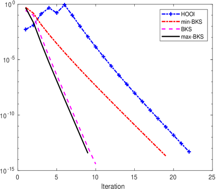
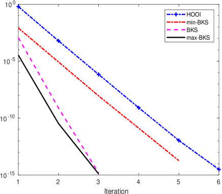
The convergence results are presented in figures, where the $y$-axis and $x$-axis represent the relative norm of G-gradient and the number of outer iterations, respectively. For the larger examples we also plot the gradient against the execution time.

In the examples we used rather small values for $(r_{1},r_{1},r_{3})$, like in some real world applications [34, 36]. In two forthcoming papers [17, 16] on tensor partitioning and data science applications we compute rank-$(2,2,2)$ approximations.

The experiments were performed using Matlab and the tensor toolbox [4] on a standard desktop computer with 8 GBytes RAM memory. In all test cases the memory was sufficient.

6.2.1 Example 1. Synthetic signal-plus-noise tensor

For the first test we generated synthetic $(1,2)$-symmetric tensors with specified low rank. Let $\mathcal{A}=\mathcal{A}_{signal}+\rho\mathcal{A}_{noise}$, where $\mathcal{A}_{signal}$ is a signal tensor with low multilinear rank, $\mathcal{A}_{noise}$ is a noise tensor and $\rho$ denotes the noise level. $\mathcal{A}_{signal}$ was constructed as a tensor of dimension $(r_{1},r_{1},r_{3})$ with normally distributed $N(0,1)$ elements; this was placed at the top left corner of a zero tensor of size $m\times m\times n$. The elements of the noise tensor were chosen normally distributed $N(0,1)$, and then the tensor was made $(1,2)$-symmetric. For testing purposes we performed a random permutation such that the tensor remained (1,2)-symmetric. This tensor is dense. The purpose of this example is to demonstrate that the rate of convergence of all methods depends heavily on the conditioning of the approximation problem (cf. [15, Corollary 4.5] and the short statement in Section 5.1).

Figure 2 illustrates the convergence results for a $200\times 200\times 200$ tensor approximated by one of rank-$(2,2,2)$, which is the correct rank of the signal tensor. The problem with $\rho=10^{-2}$ is more difficult than the other one, because the signal-to-noise ratio is smaller, making the approximation problem more ill-conditioned. This shows in the iteration count for all methods. See also Table 4, where the S-values are given. The HOOI was considerably more sensitive to the starting approximation than the other methods. For a few starting values it converged much more slowly than in the figure.

Figure 2: Convergence for Example 1 when $(m,m,n)=(200,200,200)$ and $(r_{1},r_{1},r_{3})=(2,2,2)$. In the top plot $\rho=10^{-2}$ and in the bottom $\rho=10^{-4}$. In both cases the methods min-BKS(3,4;34,25), BKS(2,4;20,13), and max-BKS(2;32,23) were used.

Table 4: Example 1. S-values for $\rho=10^{-2}$ (left) and $\rho=10^{-4}$ (right). The column $k$ is the mode.

$k$	$s_{1}^{(k)}$	$s_{2}^{(k)}$	$s_{3}^{(k)}$
1	1.95	1.33	0.11
3	2.07	1.13	0.14

$k$	$s_{1}^{(k)}$	$s_{2}^{(k)}$	$s_{3}^{(k)}$
1	1.80	1.68	0.001
3	2.43	0.35	0.001

For this small problem it is possible to compute the solution directly using HOOI and the Newton-Grassmann method, without the Krylov-Schur approach. We compared that solution with the one obtained using the max-BK method and they agreed to within less than the magnitude of the stopping criterion (the angles between the subspaces spanned by the solution matrices were computed).

For the small problems in this example it is not meaningful to compare the computational efficiency of the BKS methods to that of HOOI: due to the simplicity of HOOI, it comes out as a winner in the cases when it converges.

6.2.2 Example 2. The Princeton tensor

The Princeton tensor is created using the Facebook data from Princeton [46]. We constructed it from a social network, using a student/faculty flag as third mode: the tensor element $\mathcal{A}(\lambda,\mu,\nu)=1$, if students $\lambda$ and $\mu$ are friends and one of them has flag $\nu$. After zero slices in the third mode have been removed, this is a $6593\times 6593\times 29$ tensor with $1.2\cdot 10^{6}$ non zeros.

Figure 3 shows the convergence for the Princeton tensor approximated with a rank-$(2,2,2)$ and a $(4,4,4)$-rank tensor. In both cases the inner iterations were initialized with truncated HOSVD followed by 5 HOOI iterations.

Figure 3: Convergence for Example 2, the Princeton tensor with $(m,m,n)=(6593,6593,29)$ and $(r_{1},r_{2},r_{3})=(3,3,3)$. Convergence as function of iterations (left), as function of time (seconds), (right). The methods min-BKS(3,5;62,29), BKS(2,4;36,21), and max-BKS(1;12,9) were used.

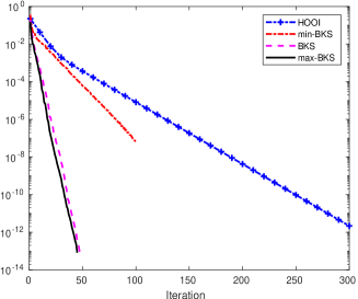
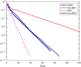
The time measurements in Figure 3 are based on the Matlab functions tic and toc. A large proportion of the time in HOOI is the computation of the G-gradient (which was done every ten iterations).

Table 5: Example 2, Princeton tensor. S-values for $(r_{1},r_{2},r_{3})=(3,3,3)$. Note that the very small entry is approximately equal to zero in the floating point system.

$k$	$s_{1}^{(k)}$	$s_{2}^{(k)}$	$s_{3}^{(k)}$	$s_{4}^{(k)}$
1	300	193	187	47.3
3	390	185	80.2	$2.4\cdot 10^{-14}$

In Table 5 we give the S-values. The mode-3 entries are a strong indication that the mode-3 multilinear rank of the tensor is equal to 3. Any attempt to compute e.g. a rank-(4,4,4) approximation will suffer from the mode-3 ill-conditioning and is likely to give incorrect results. However, a rank-(4,4,3) can be computed easily using BKS. Here the convergence of HOOI was very slow.

The number of iterations in the BKS method was rather insensitive to the choice of stage and block size parameters $s$ and $p$. Thus it did not pay off to use a larger inner subproblem. Similarly, the use of max-BKS(2;111,29) gave relatively fast convergence in terms of the number of iterations, but the extra information gained by using a large value of $k_{1}$ was not so substantial that it made up for the heavier computations.

HOOI was sensitive to the choice of starting approximation. Often the convergence rate was considerably slower than in Figure 3.

6.2.3 Example 3. The Reuters tensor

The Reuters tensor is a sparse tensor of dimensions $13332\times 13332\times 66$ with $486,894$ nonzero elements. It is constructed from all stories released during 66 consecutive days by the news agency Reuters after the September 11, 2001, attack [5]. The vertices of the network are words. There is an edge between two words if they appear in the same text unit (sentence). The weight of an edge is its frequency.

Figure 4 shows the convergence results for the Reuters tensor, approximated with a rank-$(2,2,2)$ and a rank-$(6,6,6)$ tensor. In the second case, the inflexibility of the choice of $k_{1}$ and $k_{3}$ in max-BKS forced us to use stage 1, which led to slower convergence than with BKS and min-BKS.

Figure 4: Convergence for Example 3, the Reuters tensor with $(m,m,n)=(13332,13332,66)$. Top plot: $(r_{1},r_{2},r_{3})=(2,2,2)$. The methods min-BKS(3,4;34,25), BKS(2,4;20,13) and max-BKS(2;32,23) were used. Bottom plot: $(r_{1},r_{2},r_{3})=(6,6,6)$. The methods min-BKS(2,4;58,37), BKS(1,6;42,27) and max-BKS(1;42,27) were used (the last two are identical for these parameters).

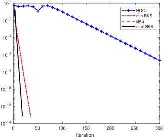
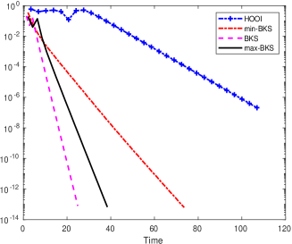
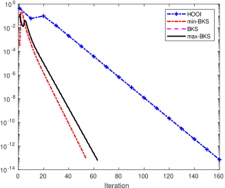
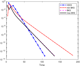
The S-values are given in Table 6. It is seen that none of the problems is particularly ill-conditioned.

Table 6: Example 3 S-values for the Reuters tensor with $(r_{1},r_{2},r_{3})=(2,2,2)$ (left) and $(r_{1},r_{2},r_{3})=(6,6,6)$ (right).

$k$	$s_{1}^{(k)}$	$s_{2}^{(k)}$	$s_{3}^{(k)}$
1	350	207	75.2
3	397	88	13

$k$	$s_{1}^{(k)}$	$\cdots$	$s_{6}^{(k)}$	$s_{7}^{(k)}$
1	353	$\cdots$	125	74.3
3	495	$\cdots$	22.2	15.7

It is argued in [17] that in cases when the 3-slices of a (1,2)-symmetric tensor are adjacency matrices of graphs, then one should normalize the slices so that the largest eigenvalue of each slice becomes equal to 1. In that context a rank-(2,2,2) approximation is computed. We ran a test with the normalized tensor and the same parameter values as in Figure 4. The results are shown in Figure 5.

Figure 5: Convergence for Example 3, the scaled Reuters tensor, and $(r_{1},r_{2},r_{3})=(2,2,2)$. We used min-BKS(3,4;34,25), BKS(2,4,32,23), and max-BKS(2;32,23).

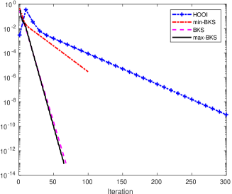
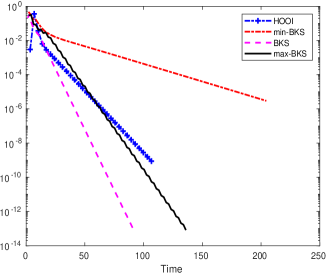
The S-values are given in Table 7. They indicate that this problem is slightly more ill-conditioned than the unscaled one.

Table 7: Example 3. S-values for the scaled Reuters tensor with $(r_{1},r_{2},r_{3})=(2,2,2)$.

$k$	$s_{1}^{(k)}$	$s_{2}^{(k)}$	$s_{3}^{(k)}$
1	5.07	3.43	0.692
3	6.11	0.421	0.222

6.2.4 Example 4. 1998DARPA tensor

The following description is taken from [16]. In [25] network traffic logs are analyzed in order to identify malicious attackers. The data are called the 1998 DARPA Intrusion Detection Evaluation Dataset and were first published by the Lincoln Laboratory at MIT. We downloaded the data set from https://datalab.snu.ac.kr/haten2/ in October 2018. The records consist of (source IP, destination IP, port number, timestamp). In the data file there are about 22000 different IP addresses. We chose the subset of 8991 addresses that both sent and received messages. The time span for the data is from June 1 1998 to July 18, and the number of observations is about 23 million. We merged the data in time by collecting every 63999 consecutive observations into one bin. Finally we symmetrized the tensor $\mathcal{A}\in\mathbb{R}^{m\times m\times n}$, where $m=8891$ and $n=371$, so that

$$a_{ijk}=\begin{cases}1&\mbox{ if }i\mbox{ communicated with }j\mbox{ in time slot }k\\ 0&\mbox{ otherwise.}\end{cases}$$

In this example we did not normalize the slices of the tensor: The 3-slices are extremely sparse, and normalization makes the rank-(2,2,2) problem so ill-conditioned that none of the algorithms converged. Instead we scaled the slices to have Frobenius norm equal to 1. The convergence history is shown in Figure 6.

Figure 6: Convergence for Example 4, the 1998DARPA tensor with $(m,m,n)=(8991,8991,371)$, and $(r_{1},r_{2},r_{3})=(2,2,2)$. The methods min-BKS(2,4;18,15), BKS(2,4;20,13) and max-BKS(2;32,23) were used.

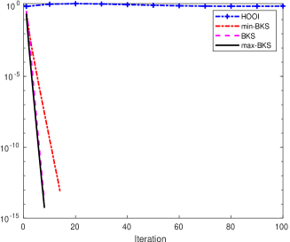
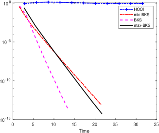
The HOOI method was sensitive to the (random) starting approximations. It did happen that the method converged rapidly, but in many cases convergence was extremely slow.

The S-values are given in Table 8. The problem is well-conditioned.

Table 8: Example 4. S-values for the 1998DARPA tensor with $(r_{1},r_{2},r_{3})=(2,2,2)$.

$k$	$s_{1}^{(k)}$	$s_{2}^{(k)}$	$s_{3}^{(k)}$
1	6.35	6.12	0.948
3	8.82	0.257	0.0995

6.2.5 Discussion of experiments

Profiling tests of the BKS and HOOI methods for the Reuters example show that most of the computational work is done in the reshaping of tensors, and in tensor-matrix multiplications. For small values of the rank $(r_{1},r_{1},r_{3})$, the number of stages and block size in the BKS methods, the time work for the dense tensor and matrix operations in the inner iterations in BKS and the SVD’s in HOOI is relatively small. A considerable proportion of the work in HOOI is the computation of the G-gradient; we reduced that by computing it only every ten iterations. The data shuffling and reshaping must be done irrespectively of which programming language is used. It is reasonable to assume that the implementation made in the sparse tensor toolbox [4] is efficient. Therefore it is makes sense to measure efficiency by comparing the Matlab execution times (by tic and toc) of the methods.

Our tests with (1,2)-symmetric tensors indicate that all methods considered here converge fast for very well-conditioned problems. However, the convergence behavior of HOOI was less predictable: sometimes it converged very slowly also for well-conditioned, large problems. Consistently the min-BKS method converged much more slowly than the other two Krylov-Schur like methods. The max-BKS method suffered from its inflexibility in the choice of $k_{1}$ and $k_{3}$, especially with $r_{1}$ and $r_{3}$ somewhat larger.

The design of BKS is to some extent based on heuristics and numerical experiments. A comparison of BKS and max-BKS shows that the choice of blocks of $p$ vectors, for $p$ rather small, in the Krylov steps, does not substantially impede the convergence rate. Using fewer blocks, in the sense of using only $p$ vectors from the “diagonal” blocks in the diagram in Table 1, as in min-BKS, leads to slower convergence. Thus BKS seems to be a reasonable compromise. Based on the experience presented in this paper and [17, 16] it seems clear that for large and sparse tensors the BKS method is in general more robust and efficient than HOOI.

In the BKS method the parameters $s$ and $p$ (which give $k_{1}$ and $k_{3}$) could be chosen rather small, typically 2 and 4, respectively. Using larger values did not pay off.

7 Conclusions and future work

We have generalized block Krylov-Schur methods for matrices to tensors and demonstrated that the new method can be used for computing best rank-$(r_{1},r_{2},r_{3})$ approximations of large and sparse tensors. The BKS method is shown to be flexible and has best convergence properties.

The purpose of this paper has been to show that the block-Krylov-Schur method is a viable approach. It may be possible to analyze BKS methods in depth, theoretically and by experiments, and optimize the method further, for instance with regard to the choice of blocks in the tables defining the method.

Since we are interested in very low rank approximation of (1,2)-symmetric tensors for applications such as those in [17, 16], the development of block Krylov-Schur type methods was done mainly with such applications in mind. More work is needed to investigate the application of BKS methods for nonsymmetric tensors.

The detailed implementation of block Krylov-Schur methods for matrices is rather technical, see e.g. [51]. The generalization to tensors might improve the convergence properties for ill-conditioned problems. However, this is beyond the scope of the present paper, and may be a topic for future research.

It appears to be straightforward to generalize the results to tensors of order larger than 3. We are planning to do research in this direction in the future.

8 Acknowledgments

This work was done when the second author visited the Department of Mathematics, Linköping University.

Appendix A The Grassmann Hessian

Let $X\in\mathbb{R}^{l\times r}$, be a matrix with orthonormal columns, $X^{\sf T}X=I_{r}$. We will let it represent an entire subspace, i.e. the equivalence class,

$$[X]=\{XQ\;|\;Q\in\mathbb{R}^{r\times r},Q^{\sf T}Q=I_{r}\}.$$

For convenience we will say that $X\in\mathrm{Gr}(l,r)$, the Grassmann manifold (of equivalence classes).

Define the product manifold

$$\mathrm{Gr}^{3}=(\mathrm{Gr}(l,r_{1}),\mathrm{Gr}(m,r_{2}),\mathrm{Gr}(n,r_{3})),$$

and, for given integers satisfying $r_{1}<k_{1}<l$, $r_{2}<k_{2}<m$, and $r_{3}<k_{3}<n$,

$$\mathrm{Gr}^{3}_{k}=(\mathrm{Gr}(k_{1},r_{1}),\mathrm{Gr}(k_{2},r_{2}),\mathrm{Gr}(k_{3},r_{3})).$$

The following is a submanifold of $\mathrm{Gr}^{3}$:

$$\mathrm{Gr}_{s}^{3}=\{(X,Y,Z)=\left(\begin{pmatrix}U\\ 0\end{pmatrix},\begin{pmatrix}V\\ 0\end{pmatrix},\begin{pmatrix}W\\ 0\end{pmatrix}\right)\in\mathrm{Gr}^{3}\;|\;(U,V,W)\in\mathrm{Gr}_{k}^{3}\}.$$

Let $(X_{0},Y_{0},Z_{0})\in\mathrm{Gr}^{3}$, and let three matrices $X_{1}\in\mathbb{R}^{l\times(k_{1}-r_{1})}$, $Y_{1}\in\mathbb{R}^{m\times(k_{2}-r_{2})}$, and $Z_{1}\in\mathbb{R}^{n\times(k_{3}-r_{3})}$ be given, such that

$$\bar{X}=[X_{0}\,X_{1}],\qquad\bar{Y}=[Y_{0}\,Y_{1}],\qquad\bar{Z}=[Z_{0}\,Z_{1}],$$

all have orthonormal columns.

For a given matrix $P\in\mathrm{Gr}(l,r)$ we let $P_{\perp}\in\mathrm{Gr}(l,l-r)$ be such that $(P\,P_{\perp})$ is an orthogonal matrix. It can be shown [11, Section 2.5] that $P_{\perp}$ is a matrix of basis vectors in the tangent space of $\mathrm{Gr}(l,r)$ at the point $P$.

In the maximization problem for $\|\mathcal{A}\bm{\cdot}\bm{\left(}X,Y,Z\bm{}\|^{2}$ on the Grassmann product manifold $\mathrm{Gr}^{3}$, we now make a change of variables by defining

$$\mathcal{B}=\mathcal{A}\bm{\cdot}\bm{\left(}(\bar{X}\,\bar{X}_{\perp}),(\bar{Y}\,\bar{Y}_{\perp}),(\bar{Z}\,\bar{Z}_{\perp})\bm{},$$

and further

$$\mathcal{C}=\mathcal{A}\bm{\cdot}\bm{\left(}\bar{X},\bar{Y},\bar{Z}\bm{}.$$

Clearly $\mathcal{C}$ is a leading subtensor of $\mathcal{B}$, see Figure 1. After this change of variables the point $(X_{0},Y_{0},Z_{0})$ is represented by

$$\mathrm{Gr}^{3}\ni E_{0}=\left(\begin{pmatrix}I_{r_{1}}\\ 0\end{pmatrix},\begin{pmatrix}I_{r_{2}}\\ 0\end{pmatrix},\begin{pmatrix}I_{r_{3}}\\ 0\end{pmatrix}\right),$$

and the bases for the tangent space of $\mathrm{Gr}^{3}$ at $E_{0}$ are

$$(E_{0})_{\perp}=\left(\begin{pmatrix}0\\ I_{l-r_{1}}\end{pmatrix},\begin{pmatrix}0\\ I_{m-r_{2}}\end{pmatrix},\begin{pmatrix}0\\ I_{n-r_{3}}\end{pmatrix}\right).$$

The bases for the tangent space of the submanifold $\mathrm{Gr}_{s}^{3}$ at $E_{0}$ are given by

$$\left(\begin{pmatrix}0\\ I_{k_{1}-r_{1}}\\ 0\end{pmatrix},\begin{pmatrix}0\\ I_{k_{2}-r_{2}}\\ 0\end{pmatrix},\begin{pmatrix}0\\ I_{k_{3}-r_{3}}\\ 0\end{pmatrix}\right),$$

where the top zeros are in $\mathbb{R}^{r_{i}\times r_{i}}$, $i=1,2,3$, and the bottom in $\mathbb{R}^{(l-k_{1})\times(k_{1}-r_{1})}$, $\mathbb{R}^{(m-k_{2})\times(k_{2}-r_{2})}$, and $\mathbb{R}^{(n-k_{3})\times(k_{3}-r_{3})}$, respectively. Clearly, the tangent space of $\mathrm{Gr}^{3}_{s}$ is a subspace of the tangent space of $\mathrm{Gr}^{3}$.

Define the functions

$$f(X,Y,Z) =\|\mathcal{B}\bm{\cdot}\bm{\left(}X,Y,Z\bm{}\|^{2},\qquad(X,Y,Z)\in\mathrm{Gr}^{3},$$

$$g(U,V,W) =\|\mathcal{C}\bm{\cdot}\bm{\left(}U,V,W\bm{}\|^{2},\qquad(U,V,W)\in\mathrm{Gr}_{k}^{3}$$

The subtensor property implies that for $(U,V,W)\in\mathrm{Gr}_{k}^{3}$,

(27) $$g(U,V,W)=f(X,Y,Z),\qquad(X,Y,Z)=\left(\begin{pmatrix}U\\ 0\end{pmatrix},\begin{pmatrix}V\\ 0\end{pmatrix},\begin{pmatrix}W\\ 0\end{pmatrix}\right).$$

Proposition A.1.

Assume that the Grassmann Hessian of $f$ is positive definite on the tangent space of $\mathrm{Gr}^{3}$ at $E_{0}$. Then the Grassmann Hessian of $g$ is positive definite on the tangent space of $\mathrm{Gr}_{k}^{3}$ at the point

$$E_{0k}=\left(\begin{pmatrix}I_{r_{1}}\\ 0\end{pmatrix},\begin{pmatrix}I_{r_{2}}\\ 0\end{pmatrix},\begin{pmatrix}I_{r_{3}}\\ 0\end{pmatrix}\right)\in\mathrm{Gr}^{3}_{k}.$$

Proof A.2.

As the tangent space in $\mathrm{Gr}^{3}_{s}$ at $E_{0}$ is a subspace of the tangent space in $\mathrm{Gr}^{3}$, the Hessian of $f$ must be positive definite at $E_{0}$ in $\mathrm{Gr}_{s}^{3}$. Therefore, due to (27), the geometric properties of $g$ are the same as those of $f$, and the Hessian of $g$ is positive definite in $\mathrm{Gr}_{k}^{3}$ at $E_{0k}$.

Appendix B Implementation of the block-Krylov step

The steps (ii)-(iv) in Algorithm 3 are written in tensor form to emphasize the equivalence to Gram-Schmidt orthogonalization. As we remarked in Section 4.3, the reorganization of data from tensor to matrix form before performing tensor-matrix multiplication is costly. Therefore, we keep the result of step (i) in matrix form and directly orthogonalize it to the previous vectors by performing a QR decomposition. Thereby we also avoid performing reorthogonalization, which might be necessary if we use the Gram-Schmidt method.

References

- [1] P.-A. Absil, R. Mahony, and R. Sepulchre, Optimization Algorithms on Matrix Manifolds, Princeton University Press, 2007.
- [2] C. A. Andersson and R. Bro, Improving the speed of multi-way algorithms: Part i. Tucker3, Chemometrics and intelligent laboratory systems, 42 (1998), pp. 93–103.
- [3] B. W. Bader and T. G. Kolda, Algorithm 862: MATLAB tensor classes for fast algorithm prototyping, ACM Transactions on Mathematical Software (TOMS), 32 (2006), pp. 635–653.
- [4] B. W. Bader and T. G. Kolda, Efficient MATLAB Computations with Sparse and Factored Tensors, SIAM Journal on Scientific Computing, 30 (2007), pp. 205–231, https://doi.org/10.1137/060676489, http://link.aip.org/link/?SCE/30/205/1.
- [5] V. Batagelj and A. Mrvar, Density based approaches to network analysis. analysis of Reuters terror news network., University of Ljubljana, Slovenia, (2003), https://repozitorij.uni-lj.si/IzpisGradiva.php?id=33150&lang=eng.
- [6] P. Comon, Tensor decompositions, Mathematics in Signal Processing V, (2002), pp. 1–24.
- [7] P. Comon and B. Mourrain, Decomposition of quantics in sums of powers of linear forms, Signal Processing, 53 (1996), pp. 93–107.
- [8] L. De Lathauwer, B. De Moor, and J. Vandewalle, A multilinear singular value decomposition, SIAM Journal on Matrix Analysis and Applications, 21 (2000), pp. 1253–1278.
- [9] L. De Lathauwer, B. De Moor, and J. Vandewalle, On the best rank-1 and rank-() approximation of higher-order tensors, SIAM Journal on Matrix Analysis and Applications, 21 (2000), pp. 1324–1342.
- [10] V. De Silva and L.-H. Lim, Tensor rank and the ill-posedness of the best low-rank approximation problem, SIAM Journal on Matrix Analysis and Applications, 30 (2008), pp. 1084–1127.
- [11] A. Edelman, T. Arias, and S. T. Smith, The Geometry of Algorithms with Orthogonality Constraints, SIAM J. Matrix Anal. Appl., 20 (1998), pp. 303–353.
- [12] A. Edelman, T. A. Arias, and S. T. Smith, The geometry of algorithms with orthogonality constraints, SIAM journal on Matrix Analysis and Applications, 20 (1998), pp. 303–353.
- [13] L. Eldén, Matrix methods in data mining and pattern recognition, SIAM, 2007.
- [14] L. Eldén and B. Savas, A Newton–Grassmann method for computing the best multilinear rank-() approximation of a tensor, SIAM Journal on Matrix Analysis and applications, 31 (2009), pp. 248–271.
- [15] L. Eldén and B. Savas, Perturbation theory and optimality conditions for the best multilinear rank approximation of a tensor, SIAM Journal on Matrix Analysis and Applications, 32 (2011), pp. 1422–1450.
- [16] L. Eldén and M. Dehghan, Analyzing large and sparse tensor data using spectral low-rank approximation, 2020, https://arxiv.org/abs/2012.07754.
- [17] L. Eldén and M. Dehghan, Spectral partitioning of large and sparse tensors using low-rank tensor approximation, 2020, https://arxiv.org/abs/2012.07689.
- [18] R. Fletcher, Practical Methods of Optimization, Wiley, 2nd ed., 1987.
- [19] G. Golub and W. Kahan, Calculating the singular values and pseudo-inverse of a matrix, Journal of the Society for Industrial and Applied Mathematics, Series B: Numerical Analysis, 2 (1965), pp. 205–224.
- [20] G. H. Golub and C. F. Van Loan, Matrix computations, Johns Hopkins University, Press, Baltimore, MD, USA, 4th ed., 2013.
- [21] S. Goreinov, I. V. Oseledets, and D. V. Savostyanov, Wedderburn rank reduction and Krylov subspace method for tensor approximation. Part 1: Tucker case, SIAM Journal on Scientific Computing, 34 (2012), pp. A1–A27.
- [22] F. L. Hitchcock, Multiple invariants and generalized rank of a p-way matrix or tensor, Studies in Applied Mathematics, 7 (1928), pp. 39–79.
- [23] M. Ishteva, P.-A. Absil, S. Van Huffel, and L. De Lathauwer, Best low multilinear rank approximation of higher-order tensors, based on the Riemannian trust-region scheme, SIAM Journal on Matrix Analysis and Applications, 32 (2011), pp. 115–135.
- [24] M. Ishteva, L. De Lathauwer, P.-A. Absil, and S. Van Huffel, Differential-geometric Newton method for the best rank-() approximation of tensors, Numerical Algorithms, 51 (2009), pp. 179–194.
- [25] I. Jeon, E. Papalexakis, C. Faloutsos, L. Sael, and U. Kang, Mining Billion-Scale Tensors: Algorithms and Discoveries, The VLDB Journal, 25 (2016), pp. 519–544, https://doi.org/10.1007/s00778-016-0427-4, https://doi-org.e.bibl.liu.se/10.1007/s00778-016-0427-4.
- [26] O. Kaya and B. Uçar, High performance parallel algorithms for the Tucker decomposition of sparse tensors, in 2016 45th International Conference on Parallel Processing (ICPP), 2016, pp. 103–112, https://doi.org/10.1109/ICPP.2016.19.
- [27] B. Khoromskij and V. Khoromskaia, Low rank Tucker-type tensor approximation to classical potentials, Open Mathematics, 5 (2007), pp. 523–550.
- [28] B. N. Khoromskij and V. Khoromskaia, Multigrid accelerated tensor approximation of function related multidimensional arrays, SIAM Journal on Scientific Computing, 31 (2009), pp. 3002–3026.
- [29] T. Kolda and J. Sun, Scalable tensor decompositions for multi-aspect data mining, in 2008 Eighth IEEE International Conference on Data Mining, 2015, pp. 363–372.
- [30] T. G. Kolda and B. W. Bader, Tensor decompositions and applications, SIAM review, 51 (2009), pp. 455–500.
- [31] T. G. Kolda, B. W. Bader, and J. P. Kenny, Higher-order web link analysis using multilinear algebra, in Fifth IEEE International Conference on Data Mining, IEEE, 2005, pp. 27–30.
- [32] R. B. Lehoucq, D. C. Sorensen, and C. Yang, ARPACK users’ guide: solution of large-scale eigenvalue problems with implicitly restarted Arnoldi methods, SIAM, 1998.
- [33] L.-H. Lim and J. Morton, Cumulant component analysis: a simultaneous generalization of PCA and ICA, CASTA2008, (2008), p. 18.
- [34] X. Liu, S. Ji, W. Glänzel, and B. De Moor, Multiview partitioning via tensor methods, IEEE Transactions on Knowledge and Data Engineering, 25 (2013), pp. 1056–1069.
- [35] I. V. Oseledets, D. Savostianov, and E. E. Tyrtyshnikov, Tucker dimensionality reduction of three-dimensional arrays in linear time, SIAM Journal on Matrix Analysis and Applications, 30 (2008), pp. 939–956.
- [36] C. Persson, L. Bohlin, D. Edler, and M. Rosvall, Maps of sparse Markov chains efficiently reveal community structure in network flows with memory, arXiv preprint arXiv:1606.08328, (2016).
- [37] M. J. Powell, On search directions for minimization algorithms, Mathematical Programming, 4 (1973), pp. 193–201.
- [38] A. Ruhe and P. Å. Wedin, Algorithms for separable nonlinear least squares problems, SIAM Review, 22 (1980), pp. 318–337.
- [39] B. Savas and L. Eldén, Handwritten digit classification using higher order singular value decomposition, Pattern recognition, 40 (2007), pp. 993–1003.
- [40] B. Savas and L. Eldén, Krylov-type methods for tensor computations I, Linear Algebra and its Applications, 438 (2013), pp. 891–918.
- [41] B. Savas and L.-H. Lim, Quasi-Newton methods on Grassmannians and multilinear approximations of tensors, SIAM Journal on Scientific Computing, 32 (2010), pp. 3352–3393.
- [42] A. Smilde, R. Bro, and P. Geladi, Multi-way analysis: applications in the chemical sciences, John Wiley & Sons, 2005.
- [43] D. C. Sorensen, Implicit application of polynomial filters in a k-step Arnoldi method, SIAM journal on matrix analysis and applications, 13 (1992), pp. 357–385.
- [44] G. W. Stewart, A Krylov–Schur algorithm for large eigenproblems, SIAM Journal on Matrix Analysis and Applications, 23 (2001), pp. 601–614.
- [45] G. W. Stewart, Matrix Algorithms: Volume II: Eigensystems, SIAM, 2001.
- [46] A. L. Traud, E. D. Kelsic, P. J. Mucha, and M. A. Porter, Comparing Community Structure to Characteristics in Online Collegiate Social Networks, SIAM Rieview, 53 (2011), pp. 526–543.
- [47] L. R. Tucker, The Extension of Factor Analysis to Three-Dimensional Matrices, in Contributions to Mathematical Psychology, H. Gulliksen and N. Frederiksen, eds., Holt, Rinehart and Winston, New York, 1964, pp. 109–127.
- [48] L. R. Tucker, Some Mathematical Notes on Three-Mode Factor Analysis, Psychometrika, 31 (1966), pp. 279–311.
- [49] Y. Xu, On the Convergence of Higher-Order Orthogonality Iteration, Tech. Report 1504.00538v2, arXiv [math.NA], 2015.
- [50] T. Zhang and G. H. Golub, Rank-one approximation to higher order tensors, SIAM Journal on Matrix Analysis and Applications, 23 (2001), pp. 534–550.
- [51] Y. Zhou and Y. Saad, Block Krylov-Schur method for large symmetric eigenvalue problems, Numer. Alg., 47 (2008), pp. 341–359.