Incorporating Domain Knowledge To Improve Topic Segmentation Of Long MOOC Lecture Videos

Abstract

Topical Segmentation poses a great role in reducing search space of the topics taught in a lecture video specially when the video metadata lacks topic wise segmentation information. This segmentation information eases user efforts of searching, locating and browsing a topic inside a lecture video. In this work we propose an algorithm, that combines state-of-the art language model and domain knowledge graph for automatically detecting different coherent topics present inside a long lecture video. We use the language model on speech-to-text transcription to capture the implicit meaning of the whole video while the knowledge graph provides us the domain specific dependencies between different concepts of that subjects. Also leveraging the domain knowledge we can capture the way instructor binds and connects different concepts while teaching, which helps us in achieving better segmentation accuracy. We tested our approach on NPTEL[1] lecture videos and holistic evaluation shows that it out performs the other methods described in the literature.

I Introduction

Online learning specially Massive Open Online Learning (MOOCs) is becoming popular as it is designed to facilitate large number of participants by providing free online access of the high quality educational contents[2]. So many MOOCs provider like NPTEL[1] offers long lecture videos having duration $\sim$1 hour. These videos contain multiple non overlapping coherent topics as they are taught by the instructor. Having an index built using these topics help user in browse, locate and searching a desired topic inside a lecture video as well as inside the whole lecture series. Usually these video metadata lacks the presence of annotated metadata, which supposed to hold the time stamp of each topics taught in these video. So for a learner, to search, locate and browse a topic inside the lecture series, (s)he needs to go through the whole lecture video, even in the worst case scenario s(he) requires to view all the video in the lecture series. Successful construction of an indexing system based on all the topics taught inside a lecture video requires to have topic name and its boundary information inside a lecture video. In order to facilitate users with a faster content search facility inside the whole course as well as in a video and for providing better learning experience, lecture video needs to be topic wise segmented and the video metatdata should have topic boundary information in the form of starting and ending time. Later an indexing framework can be easily built using these segmented topics which in turn mitigate user effort of topic wise video content search.

In literature several researchers [3, 4, 5, 6, 7] performed lecture video segmentation by measuring the structural similarity of the resources. For the text data the idea primarily revolves around dividing the whole text into fixed length overlapping text blocks and measuring the similarity between all pair of adjacent text blocks. Shah et al. [8] represented cue phrases using n-gram based language model and Galanopoulos et al. [9] used word2vec based word embedding to represent text blocks. But finally both of them applied the traditional similarity measure based approach in obtaining topic boundaries.

While on the other hand segmentation approach using video file [10, 11, 8, 12] primarily involves extracting text information from lecture slides shown inside the video and finding similarity measure in local context. These approach has following short comings.

• Similarity measure based approach require lots of fine tuning for the videos having topics with different time duration.

• Topic segmentation that uses language model may capture the the underlined meaning of the transcribed file. But it cannot captures the global semantics of the transcript file.

• Domain knowledge in not used during the segmentation task hence knowledge semantics is not captured for finding the topic boundaries.

To overcome these shortcomings, in this work we initially perform the topical segmentation using a language model. A language model tries to learn the structure of the text corpus through hierarchical representation thus learns to understand the both low-level syntactic feature and high level semantic features [13]. Though language model has some limitations of capturing the context of capturing underlined semantics of the whole text [14], topical segmentation using language model only looks into the local context of the data and unable to capture the global context resulting in an inaccurate boundary detection for the larger sized topics. To overcome this problem we additionally use a domain knowledge graph at the time of segmentation. knowledge graph contains different concepts, interconnections and relationship information among the concepts of a subjects. We leverage these knowledge present inside a knowledge graph and use it during segmentation to capture the global context of the text corpus obtained from the speech-to-text transcript file. The major advantage of using knowledge graph during segmentation is the capability of capturing the global context that can detect the topic boundaries for larger topics in more accurate manner.

So in this work we have three major contributions.

• During segmentation we use state-of-the art language model that is able to understand the implicit meaning of the text data and capture the semantics in local context which helps us in detecting segment boundaries of small sized topics.

• To capture the semantics in global context we use domain knowledge graph and leverage the knowledge present it during topical segmentation that makes possible to detect segment boundaries for larger length topics.

• Using the dependencies and relationship information available in a knowledge graph, we analyze the way instructor connects and binds different concepts to explain a topic, which helps us in getting more accurate topic boundary information.

II Literature Survey

In previous years, several research works are proposed to deal with lecture video related issues like indexing, retrieval, segmentation and annotation. To accomplish these tasks mainly textual and visual information are used. Text information are available in form of subtitle file and speech-to-text transcript . Visual information is primarily obtained from lecture video and supplementary lecture material like lecture slides . Depending on the semantic resources used, we can divide the prior work into three category. Using only textual information, visual information or using both of them.

II-A Textual Information Based Segmentation

Lin et al [3] proposed a modified version of TextTiling [15] algorithm to obtain segment boundaries from audio transcripts. Their idea is to divide the whole text transcript into fixed sized overlapping blocks. Similarity between two adjacent blocks are computed using noun phrases, verb class, pronouns, cue phrase as feature vectors. Segment boundary is considered if for a block pair, similarity score is below some experimental threshold value. Shah et al [8] adopted similar approach to predict topic transition in textual content. They used cue phrases which are represented by N-gram based model while Galanopoulos et al [9] used word2Vec [4] based word embedding to measure semantic similarity between two adjacent text blocks. In an another work Shah et al [5] modified the above mentioned approach with the help of wikipedia text. They computed similarity between a wikipedia topic and each fixed size text block obtained from sub-title file. Based on all similarity score and threshold value segment boundary was decided. In their work Repp et al [6] proposed a lecture video indexing framework by forming chain index of keywords. They extracted a set of keywords from the speech transcripts. For each keyword, using its occurrence position a keyword chain is formed. Finally time stamp of each chain is used to index the lecture video. Using Multi Modal Language Model Chen et al [7] focused to index textual data obtained from slides and speech in lecture videos, and subsequently employed a multi-modal probabilistic ranking function for lecture video retrieval. Basu et al [16] built an Lecture video recommendation system for educational blogs using topic modeling technique.

II-B Visual Information Based Segmentation

Researchers worked with visual contents, primarily focused on extracting textual information present in lecture slides and applying NLP based methods on them to find topic segment boundaries. Che et al. [11] and Baidya et al [17] analyzed textual contents available in the lecture slides shown in the lecture video. SWT was used to obtain text lines form slide frame and OCR is used to recognize text data from these text lines. NLP based methods are applied on text data to perform topic segmentation. Yang et al [10] used similar approach as above but used DCT based coefficient to identify text lines in a slide frame. Che et. al [11] segmented lecture video with synchronized slides. By analyzing it’s OCRed text they partition the slides into different subtopics by examining their logical relevance. Slides are synchronized with the video stream, the subtopics of the slides indicate exactly the segments of the video. Another group of researches tried to match between video frames and lecture slides, assuming that lecture slides are available as supplementary material. Eberts et al. [18] matched between lecture slides and video frames to create localization information of each slide shown in the lecture video. They leverage alignment of the presentation with the reading order of its supplementary material. They handled it by using a combination of SIFT local feature and temporal model. As temporal model they used Hidden Markov Model and heuristic filters. Ma et al. [19] Analyzed lecture slides to get topic segments. These segment boundaries are mapped to the lecture video by matching lecture slides and video frames. They handled different perspective views, resolution, illumination, noise, and occlusions in videos by using boosted margin maximizing neural networks. In some work, a lecture video is considered as a sequence of events like displaying lecture slides or the instructor. Assuming change of event as the change of current topic, topic boundary is determined by detecting the event change. Shah et al. [8] detected event change in lecture videos and considered change of an event is change of a topic. They consider events as displaying instructor or displaying lecture slide in the video. To detect event change they trained an SVM by computing color histogram of video frames. Jeong et al. [12] handled lecture video where recording was done by a non stationary camera settings. They identified topic change by computing frame similarity between two adjacent frames. based on some threshold value topic boundary was identified. Ma et al [20] used color histogram of video frames to identify slide transition, which in turn is used to detect topic change.

II-C Joint Approach of Segmentation

To obtain more accurate result researchers adopted fusion based method, which involves merging two sets of segmentation information obtained from heterogeneous sources like speech transcripts, video content, subtitle file or OCRed text. Basic idea behind the fusion approach is replacing two segment boundaries by their average transition time if two transition occurs within thirty seconds. Shah et al. [8, 5] used both subtitle file and video frames and wikipwdia text to get final segmentation. In [21] content based lecture video retrieval system is proposed by extracting keywords from slide text line and analyzing OCR and ASR transcripts of the video.

III Methodology

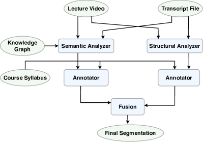
Different steps to perform topical segmentation of long lecture videos are mentioned below and the schematic diagram is shown in the Figure 1.

1. Segmentation using structural analysis In this method of lecture video segmentation first we segment the transcript file associated with a lecture video. During segmenting the transcript file we analyze the structure of the textual information and try to understand the implicit meaning of the whole transcript file. For understanding the transcribed language we train a language model and reuse it during the actual segmentation work. After we obtain the segmentation in transcript file domain we reversely map it to the lecture video domain. Section IV describes detail steps of this task.

2. Segmentation using Semantic Analysis In this step we try to obtain topic boundary information by leveraging the knowledge semantics present inside a domain knowledge graph. Also we capture the underlined meaning of the transcript file by using a state-of-the art language model. Section V describes step by step procedure to perform semantic analyzing for obtaining the topic boundaries.

3. Annotation To distinguish a segmented topic from others and to make them searchable we need to asisgn a name to each of the segmented video. We call this step as segment annotation. we create annotation module whose responsibility is to determine topic name with the help of course syllabus and lecture videos. Details annotation process are described in Section VI.

4. Fusion As mentioned earlier we get two set of topic boundary information. One using by structural analysis of the transcript file and another set of boundary information is obtained from semantic analysis based segmentation which essentially leverages domain knowledge from a knowledge graph. In this step we fuse these two set of boundary information to obtain better segmentation results. The fusion step is described in details in Section VII

Figure 1: Schematic diagram of the methodology

IV Segmentation Using Structural Analysis

The basic idea behind the structural segmentation is to identify few sentences those can be considered as topic boundaries. For doing this, we can consider a transcript file as a sequence of sentences, where each sentence consists of fixed number of words. Now semantic segmentation of text can be formulated as a binary classification problem. Given a sentence ${S_{K}}$ with K sentences ${S_{0},S_{1},....,S_{K-1}}$ preceding it and K sentences ${S_{K+1},S_{K+2},....,S_{2K}}$ following it, we need to classify whether sentence ${S_{K}}$ is the beginning of a segment or not. To represent each sentence in vector form we use InferSent [22] approach. Next, each encoded sentence along with its K-sized left and right contexts are fed to a classifier, whose output helps us to determine segment boundaries of each topic. After segment boundaries are detected in transcript file we use them for finding the topic boundary in the lecture video. We perform the following steps to accomplish the segmentation task.

IV-A Sentence Encoding

IV-A1 Sentence Encoding

We first divide the whole transcript file into strings of fixed length ($20$ words). To create sentence encoding we have used pre-trained sentence encoder model proposed by InferSent [22]. It tries to build a universal sentence encoding by learning the sentence semantics of Stanford Natural Language Inference (SNLI) [23] corpus. SNLI corpus contains $570K$ human generated English sentence pairs. Each sentence pair is manually labeled and belongs to one of the three categories: entailment, contradiction and neutral. These corpus are used to train a classifier on top of a sentence encoder, which encodes both the sentences in a sentence pair in similar manner. Semantic relationship between these two sentence vectors are computed which is turn passed through a dense layer and soft-max layer. Finally the model classifies the sentence pair among one of the three mentioned categories. Conneau et al. [22] adopted a bi-directional LSTM with a max-pooling operator as sentence encoder. In our task we use this pre-trained sentence encoder model to create sentence vectors, which are used in later stages.

IV-B Sentence Classification

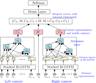
At this stage we decide, given a sentence with its $K$ sized left and right contexts, whether the sentence is the beginning of a segment or not. Our classification approach is similar in spirit of the method proposed by Badjatiya et al. [24] with some modifications. Relationship of a sentence with its left and right contexts, plays most important role to become the sentence as the segment boundary. Hence, first we compute context vectors of left and right contexts using stacked bi-LSTM with an attention layer. In stacked bi-LSTM multiple layers of both forward and backward pass LSTM [25] are stacked upon together to obtain better accuracy. Also two sentences located at equal distance, one in the left context and other on the right, might not have similar impact on the middle sentence to be it the segment boundary. To handle this we apply a soft attention layer on top of the bi-LSTM layer. Attention allows to assign different weights to the different sentences resulting better model accuracy. We define attention vector, $Z_{s}$ as

$e_{i}^{K\times 1}=H_{i}^{K\times d}\times W^{d\times 1}+b_{i}^{K\times 1}$ , $a_{i}=exp(tanh(e_{i}^{T}Z_{s}))$, $\alpha_{i}=\frac{a_{i}}{\sum_{p}a_{p}}$, $v_{i}=\sum_{j=1}^{K}\alpha_{j}h_{j}$

where, $d$ is the dimension of the output vector of last bi-LSTM layer, $H$ is the output of the bi-LSTM layer, $W$ and $b$ are the weight matrix and bias vector and $v_{i}$ is the resultant context embedding. After computing both the context vector in similar manner, we find semantic relatedness between left context (let it be $C_{L}$), right context ($C_{R}$) and the middle sentence ($M$) by the following way.

1. Concatenation of three representation $(C_{L},M,C_{R})$

2. Pair wise multiplication of the vectors $(C_{L}*M,M*C_{R},C_{R}*C_{L})$

The resultant vector which contains relationship information among these vectors, is fed to a binary classifier consists of fully connected layers culminating in a soft-max layer. The architecture diagram of this approach is is shown in Figure 2. Sentences classified as segment boundaries are used to obtain topic boundary in next step.

Figure 2: Sentence Classifier

IV-C Text To Video Mapping

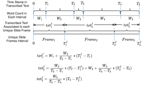
In this step, having segment boundaries obtained from text transcript, we need to identify corresponding time stamp in the original lecture video. These identified time stamps will act as starting time and ending time of different topics. We take help from text to video mapping information present inside speech-to-text transcript. Mapping information is available in the following form. After some random sentence it contains time stamp information when it is pronounced by the instructor in the lecture video. A sample of such file is shown in 4. We perform text to video mapping in the following way. Consider two consecutive time stamps $t_{S}$ and $t_{S+1}$ are given in the text transcript. Let, there exists $W$ words in between these two time stamps. Say, we get a segment boundary (in form of a sentence) inside this window. If there are $W_{p}$ words preceding this sentence, then video time stamp corresponding to this sentence is $\frac{t_{S+1}-t_{S}}{W}*W_{p}$. For a lecture video if we get $N$ ($TS_{1}$, $TS_{2}$, $TS_{3}$ … $TS_{N}$) such time stamp, then we conclude that the video contains $N-1$ topic with starting and ending time pair as ($TS_{1},TS_{2}$), ($TS_{2},TS_{3}$) …. ($TS_{N-1},TS_{N}$).

Figure 3: Sample illustration of finding transcribed text associated to each unique slide frame.

Figure 4: Mapping Information Sample: Time stamp in shown in the red box

IV-D Model Training and Parameter Tuning

To train sentence classifier we use Wikipedia [26] pages. Section boundaries in the Wikipedia pages are considered as segment boundaries. We neglect the introduction section of each page, as it briefs the overall idea of the whole page. We have randomly chosen $\sim$300 Wikipedia pages having $\sim$55K sentences, with $\sim$8% sentences being the segment boundaries. We handle this highly imbalanced dataset by selecting weighted binary cross entropy loss function, which gives higher weight to the minority class and lower weight to the majority class. This loss function $\ell$, can be defined as,

$$\ell=-\frac{1}{N}\Sigma_{n=1}^{N}w_{n}(t_{n}log(o_{n})+(1-t_{n})log(1-o_{n}))$$

where, $w_{n}$: weighting factor associated with loss of a class. $t_{n}\in{0,1}$: Binary label of the target class. $o_{n}\in[0,1]$: Classification probability score produced by the model. $N$: Total number of class, here $N=2$

We use AdaDelta [27] optimizer with dropout $0.3$. Epoch size is chosen as $35$ and the model is trained with mini batch size as $40$.

V Segmentation Using Semantic Analysis

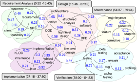
THe basic idea of this approach is to perform topical segmentation of long lecture videos by leveraging the inherent knowledge available in a domain knowledge graph($\mathscr{KG}$). Also, at the time of teaching, instructor has his own way of selecting different concepts, connecting and combining them together to explain a topic. We combine these two information to perform topical segmentation of long MOOC lecture videos. We take NPTEL lecture videos, each of them is synchronized with lecture slides and associated with speech-to-text transcript. We identify unique slides shown in the video, their time interval and associated textual information from the transcript file. Using these information we construct graphlets, each represents a unique lecture slide shown in the lecture video. In each graphlet, the nodes are the concepts used by the instructor, an edge indicates presence of a direct connection between two concepts in the $\mathscr{KG}$ and edge weight represents the contextual semantic similarity between two adjacent concepts of that edge. Here ‘contextual semantic similarity’ means semantic similarity between two concepts in the context of the way instructor combines them together during teaching. The basis of our work is to analyze all these graphlets and find how concept change occurs between two adjacent graphlets. Finally, measuring the amount of concept change and contextual semantic similarity among concepts, our system provides boundaries (starting-time and ending-time) of different topics taught in a lecture video. The idea is schematically shown in Figure 5 where we take a lecture video on ‘Overview of waterfall model’. The diagram represents different concepts used by the instructor which are distributed into five different topics. Connectivities between these concepts are taken from the $\mathscr{KG}$ and edge weight represents contextual semantic similarity among concepts. After analyzing all the graphlets created from the unique slides, we can perform topical segmentation and mark the topic boundaries.

Figure 5: Illustration of knowledge graph based topical segmentation of lecture videos. All the concepts covered in a lecture video are shown. Edge weight represents contextual semantic similarity among the concepts. Each topic, represented as a cloudy shape, consists of multiple concepts. Text in each rectangular box represents corresponding topic name and its interval.

Steps to perform segmentation using semantic analysis are described below.

V-A Edge Weight Computation

In this step, we compute the edge weight between different concepts present in the $\mathscr{KG}$. Essentially, edge weight represents how two concepts are semantically similar with each other in the context of transcript file. We find semantic similarity between them considering the context of their co-occurrence. To determine the context we use FLAIR [28] api that runs on top of the BERT [29] model. Unlike static word embedding, BERT can produce dynamic word embedding considering the sentences in which a word has occurred. Here in our work, we capture the contextual semantic similarity between two concepts, so that we can analyze how instructor correlates and connects different concepts during teaching. We observe, a concept might occur multiple times in the transcript file. So, during similarity score computation, we consider all pairwise co-occurrences between two given concepts. We take the text chunk that contains first such co-occurrence and send it to the FLAIR api to find $2048$ dimensional word embedding of each concept and calculate cosine similarity between them. We take all the co-occurrences between any two concepts, find multiple similarity scores between them and take the average to find final contextual similarity between them. After similarity computation is done, we use it as the edge weight in the $\mathscr{KG}$ if there exist a link between these two concepts. We maintain a dictionary which holds the contextual semantic similarity score between all pair of concepts present in the transcript file.

V-A1 Slide Graph Construction

First we construct an un-directed weighted graph representing each unique slide frame and we call it slide_graph. To construct $n^{th}$ slide_graph ($G^{s}_{n}$) we use transcribed text (say, $TXT_{n}$) associated with $n^{th}$ unique slide, the $\mathscr{KG}$ and the edge weight dictionary created in Section V-A. Construction steps are given below.

1. A vertex is created for each concept word in $TXT_{n}$, set vertex name as the concept and vertex weight as the term frequency of that concept in $TXT_{n}$.

2. We draw an edge between two vertices if there is a corresponding edge present in the $\mathscr{KG}$. Edge weight is assigned using the dictionary created in Section V-A.

3. We remove direction information from the generated graph because during graph analysis in the next phase, a node may not be reachable from the other nodes, though there exists a strong connection among them.

4. If the generated graph is not connected, we draw an edge between two connected components whose weight is the maximum among all the possible edges between these two components.

V-B Finding Potential Topic Boundary

In this step, we determine potential topic boundaries by analyzing all the slide_graph. During lecture, instructor changes current slide at the time of going to a different topic, but vice versa is not necessarily true. In fact usually multiple slides are used for explaining a particular topic and few consecutive slides are closely related. Here closely related means, these consecutive slides represent almost same concepts. In this step we identify closely related consecutive slides and merge them together. Also, we mark the slides which are not close and those slide changes might be the topic boundaries. We measure how much concept changes have been occurred between two consecutive lecture slides. We define concept_change_score, $CCS(j,j+1)$ between two consecutive slide_graph, $G^{s}_{j}=(V^{s}_{j},E^{s}_{j})$ and $G^{s}_{j+1}=(V^{s}_{j+1},E^{s}_{j+1})$ as follows.

$$CCS(j,j+1)=\left\{\begin{array}[]{lr}0~{}~{}~{}~{}:\{V^{s}_{j}\cap V^{s}_{j+1}\}=\phi\\ \frac{total~{}minimum~{}term~{}frequency}{total~{}maximum~{}term~{}frequency}~{}~{}~{}~{}:Else\end{array}\right.$$

where, $total~{}minimum~{}term~{}frequency=\sum\limits_{k=0}^{N}min(tf(v_{k}\mid v_{k}\in V^{s}_{j}),tf(v_{k}\mid v_{k}\in V^{s}_{j+1}))$

$total~{}maximum~{}term~{}frequency=\sum\limits_{k=0}^{M}max(tf(v_{k}\mid v_{k}\in V^{s}_{j}),tf(v_{k}\mid v_{k}\in V^{s}_{j+1}))$

where, $N=|\{V^{s}_{j}\cap V^{s}_{j+1}\}|$ and $M=|\{V^{s}_{j}\cup V^{s}_{j+1}\}|$ and $tf(v_{k}|v_{k}\in V^{s}_{j})$ indicates term frequency of vertex $v_{k}$ when $v_{k}\in V^{s}_{j}$. Here consideration of term frequency is important. We observe that, instructor puts more emphasis on few concepts while other concepts are used for giving example or reference purpose. Throughout this paper we call them as primary and auxiliary concepts respectively. Usually, primary concepts have higher term frequency than the auxiliary concepts. Also, Concepts with higher term frequency indicates that instructor has spent more time on them than the concepts with lower term frequency. Leveraging this fact we consider term frequency in concept_change_score computation. Clearly concept_change_score is in range between $[0,1]$ and its value is $1$ if two consecutive slide_graph are exactly similar and $0$ if their vertices are disjoint. An illustrative example of concept_change_score is shown in Figure 6.

Figure 6: An example of concept_change_score between two consecutive slide_graph. Each node represents a concept and its term frequency, edge weights indicate contextual semantic similarity among concepts. Slide changes shown in Figure 6 is a potential candidate of being a topic boundary as most of the concepts are different and $CCS(j,j+1)$ is low ($0.077$). While, Figure 6 shows $G^{s}_{j}$ and $G^{s}_{j+1}$ are closely related as most of the concepts present in these two slides are same and $CCS(j,j+1)$ is large ($0.545$) compared to the other.

We use this concept_change_score to identify consecutive slide_graph where significant amount of concept change happens and mark those slide transitions as potential topic boundaries. We also identify closely related consecutive slide_graph and merge them together as those corresponding slides represent almost same concepts. Steps to perform these operations are,

1. We compute concept_change_score between all pair of consecutive slide_graph and select those changes where the concept_change_score is less than the average value. We mark these changes as potential topic boundaries.

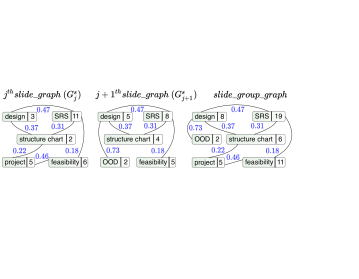
2. We merge those pair of consecutive slide_graph where concept_change_score is higher than the average value. We call this merged graph as slide_group_graph. A sample illustration of constructing slide_group_graph is shown in Figure 7.

3. slide_graph merging policy is as follows. Consider two consecutive slide_graph, $G^{s}_{j}=(V^{s}_{j},E^{s}_{j})$ and $G^{s}_{j+1}=(V^{s}_{j+1},E^{s}_{j+1})$ which are merged to get slide_group_graph, denoted as, $G^{g}=(V^{g},E^{g})$. where, $V^{g}=V^{s}_{j}\cup V^{s}_{j+1}$ and $E^{g}=E^{s}_{j}\cup E^{s}_{j+1}$. Vertex weight is modified as the summation of its weight in $G^{s}_{j}$ and $G^{s}_{j+1}$.

Figure 7: Merging two consecutive slide_graph to construct a slide_group_graph.

V-B1 Finding Actual Topic Boundary

In this step we have a collection of slide_graph and slide_group_graph. We call each of them as cluster where each of them represents some concepts and transition from one cluster to the next one makes substantial amount of concept change. Some of these transitions are actual topic boundaries while others are not. To find actual topic boundaries, we analyze how concepts are closely connected with each other within a topic than the concepts belonging in two different topics.

Primary and auxiliary concepts In our dataset we observe, in each cluster, instructor primarily focuses on some concepts and rest are used for explanation or reference purpose. We call them as primary concepts and auxiliary concepts respectively. For example, to explain a topic, say “Agile Methods”, instructor primarily focuses on concepts like, “sprint”, “scrum”, “eXtreme Programming”, “face-to-face conversation” etc. But sometimes he also mentions “waterfall”, “spiral” for reference purpose or “Zoho Sprints”, “Kanbanize” to mention the tools used for agile. We also find that term frequency of primary concepts are higher than the auxiliary concepts. Leveraging this fact, we take only the primary concepts and their interconnection for finding actual topic boundaries. we create cluster_centroid from each cluster which represents the primary concepts and the interconnections among them. In this computation we consider top 70% concepts as primary concepts. We discuss the selection of this value in Section VIII-C . Steps to construct a cluster_centroid are given below.

1. Sort the concepts in non increasing order according to their term frequency.

2. In case of tie in term frequency, we consider total weight of the incident edges to a concept. Here higher weight signifies a concept is semantically closer to other concepts than that of the concept with lower weight in incident edges.

3. Consider top $70\%$ concepts and their interconnecting edges during formation of the cluster_centroid.

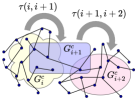
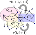
To detect actual topic boundaries, we consider three consecutive (say, $i^{th}$, $i+1^{th},$ and $i+2^{th}$) cluster_centroid denoted as $G^{c}_{i}=(V^{c}_{i},E^{c}_{i})$ , $G^{c}_{i+1}=(V^{c}_{i+1},E^{c}_{i+1})$ and $G^{c}_{i+2}=(V^{c}_{i+2},E^{c}_{i+2})$ respectively. We represent the transition from $G^{c}_{i}$ to $G^{c}_{i+1}$ as ${\tau(i,i+1)}$ and from $G^{c}_{i+1}$ to $G^{c}_{i+2}$ as ${\tau(i+1,i+2)}$. We may encounter three different cases as described below. An illustrative diagrams are also shown in Figure 8, Figure 9, and Figure 10. These figures contains small dots that represent different concepts and lines connecting them are the edges. Cloudy, rectangular and oval shapes represent three consecutive cluster_centroid $G^{c}_{i}$, $G^{c}_{i+1}$ and $G^{c}_{i+2}$ respectively. Thick gray arrows represent the transition from one cluster_centroid to the next one.

1. Case A: If we find both $\{V^{c}_{i}\cap V^{c}_{i+1}\}=\phi$ and $\{V^{c}_{i+1}\cap V^{c}_{i+2}\}=\phi$, we mark ${\tau(i,i+1)}$ as a topic boundary. This situation is represented in the Figure 8.

   

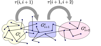
   Figure 8: An illustration of a scenario (Case A), occurs during teaching.

2. Case B: $G^{c}_{i}$ and $G^{c}_{i+2}$ are in two different topics (say, $topic_{x}$ and $topic_{y}$ in chronological order). Instructor gradually changes from $topic_{x}$ to $topic_{y}$ through $G^{c}_{i+1}$. Different situations may occur like,

   1. Situation-1 Most of the concepts covered in $G^{c}_{i+1}$ are part of $topic_{x}$, hence $\tau(i+1,i+2)$ is a topic boundary as shown in Figure 9(a).

   2. Situation-2 Most of the concepts covered in $G^{c}_{i+1}$ are part of $topic_{y}$, hence $\tau(i,i+1)$ is a topic boundary as shown in Figure 9(b).

   

   (a) Case B: Situation-1

   

   (b) Case B: Situation-2

   Figure 9: An illustration of the scenario (Case B), occurs during teaching.

3. Case C: $G^{c}_{i}$, $G^{c}_{i+1}$ and $G^{c}_{i+2}$ all falls under same topic.

   1. Situation-1 There are some changes in concepts between $G^{c}_{i}$ and $G^{c}_{i+1}$, but in $G^{c}_{i+2}$ instructor again back to the concepts present in $G^{c}_{i}$ as shown in Figure 10(a).

   2. Situation-2 Most of the concepts covered in a particular topic are present in $G^{c}_{i}$ and very few additional concepts are taught in $G^{c}_{i+1}$ and $G^{c}_{i+2}$ as shown in Figure 10(b).

   3. Situation-3 Similar to the Case C: Situation-2, while most of the concepts are covered in $G^{c}_{i+1}$as shown in Figure 10(c).

   4. Situation-4 Similar to the Case C: Situation-2, while most of the concepts are covered in $G^{c}_{i+2}$ as shown in Figure 10(d).

   

   (a) Case C: Situation-1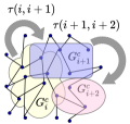

   

   (b) Case C: Situation-2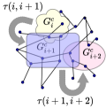

   

   (c) Case C: Situation-3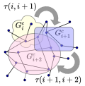

   

   (d) Case C: Situation-4

   Figure 10: An illustration of the scenario (Case C), occurs during teaching.

To handle these situations, we measure how different concepts are densely connected to each other within a topic. For a graph $G$, we define graph density metric $\delta(G)$ as, $\delta(G)=\frac{\sum_{k=1}^{N}w(e_{k})}{N(N-1)}$, while, $w(e_{k})$ is the weight of edge $e_{k}$ and $N$ is the total number of vertices in $G$. We take different combinations of cluster_centroid, compute their density and compare these density values with each other to find the actual topic boundaries. Here the idea is, concepts belong in same topic have more contextual semantic similarity than they are in different topics. Combined graph, denoted as, $\mathcal{C}(G^{c}_{i},G^{c}_{i+1})=(V^{\prime},E^{\prime})$ is formed by combining $G^{c}_{i}=(V^{c}_{i},E^{c}_{i})$ and $G^{c}_{i+1}=(V^{c}_{i+1},E^{c}_{i+1})$ where, $V^{\prime}=\{V^{c}_{i}\cup V^{c}_{i+1}\}$ and $E^{\prime}=\{E^{c}_{i}\cup E^{c}_{i+1}\cup\mathcal{E}\}$. Here, $\mathcal{E}$ represents set of additional edges present in the $\mathscr{KG}$ between any pair of concepts that belongs in $G^{c}_{i}$ or $G^{c}_{i+1}$. Using these density measure we compute actual topic boundaries using the algorithm shown in Algorithm 1.

Algorithm 1 Compute Topic Boundary List

1:$tpBoundaries\leftarrow[~{}],start\_time\leftarrow centroidList[0].startTime,end\_time\leftarrow 0,i\leftarrow 0$

2:$len\leftarrow centroidList.length$

3:while $i<len-2$  do

4:    $c0\leftarrow centroidList[i],~{}c1\leftarrow centroidList[i+1],~{}c2\leftarrow centroidList[i+2]$

5:    if $c0.vertices\cap c1.vertices=\phi~{}\textbf{and}~{}c1.vertices\cap c2.vertices=\phi$ then $\triangleright$ Case A

6:         $end\_time\leftarrow c0.endTime$

7:         $tpBoundaries\leftarrow tpBoundaries\cup(start\_time,end\_time)$ $\triangleright$ ${\tau(i,i+1)}$ is topic boundary

8:         $start\_time\leftarrow c1.startTime$ $\triangleright$ set start_time value for the next topic

9:         $i\leftarrow i+1$

10:         $continue$     
$\triangleright$ compute density of different combination of cluster_centroid as described

11:    $m01\leftarrow combine(c0,c1),~{}delta01=density(m01)$

12:    $m02\leftarrow combine(c0,c2),~{}delta02=density(m02)$

13:    $m12\leftarrow combine(c1,c2),~{}delta12=density(m12)$

14:    $m123\leftarrow combine(c1,c2,c3),~{}delta123=density(m123)$

15:    if $delta02>delta01~{}\textbf{and}~{}delta02>delta12$ then $\triangleright$ Case C: Situation-1

16:         $i\leftarrow i+2$

17:         $continue$

18:    else if $delta123>delta01~{}\textbf{or}~{}delta123>delta12~{}\textbf{or}~{}delta123>delta02$ then $\triangleright$ Case C: Situation-2,3,4

19:         $i\leftarrow i+2$

20:         $continue$

21:    else if $delta01>delta12$ then $\triangleright$ Case B: Situation-1

22:         $end\_time\leftarrow c1.endTime$

23:         $tpBoundaries\leftarrow tpBoundaries\cup(start\_time,end\_time)$ $\triangleright$ ${\tau(i+1,i+2)}$ is topic boundary

24:         $start\_time=c2.startTime$ $\triangleright$ set start_time value for the next topic

25:         $i\leftarrow i+2$

26:         $continue$

27:    else if $delta12>delta01$ then $\triangleright$ Case B: Situation-2

28:         $end\_time\leftarrow c0.endTime$

29:         $tpBoundaries\leftarrow tpBoundaries\cup(start\_time,end\_time)$ $\triangleright$ ${\tau(i,i+1)}$ is topic boundary

30:         $start\_time\leftarrow c1.startTime$ $\triangleright$ set start_time value for the next topic

31:         $i\leftarrow i+1$

32:         $continue$     

33:$end\_time\leftarrow centroidList[len-1].endTime$ $\triangleright$ taking end-time of last cluster

34:$tpBoundaries\leftarrow tpBoundaries\cup(start\_time,end\_time)$

35:return $tpBoundaries$

Lines 5-10 handle Case A by computing vertex intersection between three consecutive cluster_centroid and mark ${\tau(i,i+1)}$ as topic boundary. Case B and Case C are determined by comparing density of different combined graph formed by $G^{c}_{i}$, $G^{c}_{i+1}$ and $G^{c}_{i+2}$. For Case B:Situation-1, graph density of $\mathcal{C}(G^{c}_{i},G^{c}_{i+1})$ is more than density of $\mathcal{C}(G^{c}_{i+1},G^{c}_{i+2})$ as $G^{c}_{i}$ and $G^{c}_{i+1}$ both belong in same topic and $G^{c}_{i+1}$ and $G^{c}_{i+2}$ belong in two different topics. Hence ${\tau(i+1,i+2)}$ is a topic boundary. These are handled in lines 21-26. In similar manner Case B:Situation-2 is handled in lines 27-32. In Case C:Situation-1, concepts covered in $G^{c}_{i}$ and $G^{c}_{i+2}$ are almost similar but there is some concept change in $G^{c}_{i+1}$. So $\mathcal{C}(G^{c}_{i},G^{c}_{i+2})$ will have higher density value than that of $\mathcal{C}(G^{c}_{i+1},G^{c}_{i+2})$ and $\mathcal{C}(G^{c}_{i},G^{c}_{i+1})$ which is handled in lines 15-17. For Case C:Situation-2,3,4 all $G^{c}_{i}$,$G^{c}_{i+1}$ and $G^{c}_{i+2}$ are in same topic, so density of $\mathcal{C}(G^{c}_{i},G^{c}_{i+1},G^{c}_{i+2})$ is higher than the individual density of $\mathcal{C}(G^{c}_{i},G^{c}_{i+1})$ or $\mathcal{C}(G^{c}_{i},G^{c}_{i+2})$ or $\mathcal{C}(G^{c}_{i+1},G^{c}_{i+2})$. These kind of situations are handled in lines 18-20.

VI Annotation

At this stage we assign topic name to each video segment obtained from previous stage. We describe step by step procedure to accomplish this task using both visual and textual semantic resources, the video file and the topic name list.

VI-1 Text Line Identification and Recognition

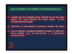
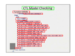
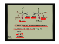
In this step we extract text line from each unique slide frames. Text Line identification is done using Stroke Width Transform (SWT) [30]. SWT is an local image operator that computes the width of the most likely stroke of a pixel and this operation is done for all the pixel. The output of SWT is an image equal to the input image size, each element contains the width of the stroke associated with the pixel. Then, by leveraging some natural observations on text line like, it appears in linear form, similarities in stroke width of the characters, letter width, height and spaces between the letters and words, SWT creates a bounding box surrounding each text line. Next, cropped text line images are passed to an OCR engine for text recognition. Open source OCR library tessaract [31] is used for it. Some slide images with detected text lines are shown in figure 11.

Figure 11: Some sample slides with identified text line with detecting title (green box) and non-title (red box)

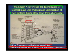
VI-2 Determine Topic Name

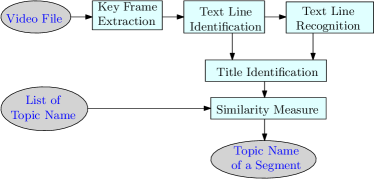
For a video segment, this step finds proper topic name using the course syllabus and identified slide titles. First we remove duplicate titles, punctuation marks and apply lemmatization on each slide title. Let us assume, within time stamp $TS_{p}$ and $TS_{q}$ we get $N$ unique titles denoted as $t_{1}$, $t_{2}$ … $t_{N}$. Now for each topic name, we measure cumulative similarity score between that topic name and all $N$ titles. Topic name that have highest cumulative similarity score is assigned to this video segment. Once a topic name is assigned, we remove that name from the topic name list so that same name is not assigned to multiple video segment. Word Mover’s Distance [32] is used for similarity measure. Using these methods we can successfully annotate each video segment obtained previously. Schematic diagram of annotation process is shown in Figure 12

Figure 12: Schematic diagram of the annotation process

VII Fusion

In this step we have two set of segmentation result obtained from two different approach mentioned above i.e. using structural analysis of the transcript file an another is from analyzing the knowledge semantics of the transcribed text leveraging domain knowledge graph. We found that structural analysis base segmentation approach performs well for small length topic segments while for large length segments this approach misses the segment boundary by large margin that reduces the overall accuracy of the topic segmentation. The situation becomes even worse for the lecture videos which mostly have comparative large topic segments. Experimental results of this shown in Section VIII-B. To alleviate this problem we use segmentation list obtained from both the approach to create the final segmentation result. Our result merging approach is given as follows.

1. For small length topic segments, we take average starting time and ending time from both the segmentation results to make the final results.

2. For large length topic segments, we discard the segmentation information obtained from the syntactic structure based result and only consider the results obtained from the semantic analysis.

Now, we need to determine the threshold value for deciding small sized topic segments and large sized topics. We take this value as $15$ minutes. We select this value experimentally and the related experiments are shown in the Section VIII-C.

VIII Experiments

VIII-A Dataset ans Ground Truth

In this work we use NPTEL lecture videos. These videos are freely available in NPTEL website. The dataset has the following properties.

1. NPTEL offers different courses, each contains $\sim$40 one hour long lecture videos.

2. Each lecture video contains $\sim$40 one hour long lecture videos. Each video is synchronized with lecture slides, i.e. at the time of lecture, instructor uses power-point/beamer presentation which is displayed in the video.

3. Each video is associated with speech-to-text transcript file. NPTEL also maintains course syllabus containing different topics taught in the whole course.

4. Usually each video consists of multiple topics taught sequentially and each topic constitutes of multiple concepts as chosen by the instructor.

5. For evaluate the structural segmentation approach we select $10$ different subjects from engineering discipline and take $10$ lecture videos from each of them. The subject name and the corresponding topic counts are shown in the Table  I.

   TABLE I: Sample Ground Truth

   Subject Name	Topic Count
   Digital Image Processing	74
   Data Structures and Algorithms	61
   Design Verification and test of Digital VLSI Designs	54
   Principles of Physical Metallurgy	79
   Cryptography and Network Security	57
   Low Power VLSI Circuits and Systems	57
   Building Materials and Construction	88
   Optimal Control Guidance and Estimation	62
   Advanced Control System Design	72
   Industrial Engineering	65

6. For evaluating semantic segmentation we take $65$ lecture videos from $2$ courses from software engineering having $255$ topics as shown in Table II.

   TABLE II: Sample Ground Truth

   Subject Name	Topic Count
   Fundamentals of embedded software testing	102
   Software Engineering	155

Ground truth are prepared by the course instructor and/or teaching assistants of the corresponding courses. Ground truth is prepared by consulting the lecture videos and the course syllabus available in NPTEL website. Ground truth of a lecture video consists of several topics along with their start-time and end-time. An overview of the ground truth is shown in Table III.

TABLE III: Sample Ground Truth

Topic Name	Start time (mm : ss)	End time (mm : ss)
Requirement Analysis	00:32	15:43
Design	15:46	27:12
Implementation	15:46	37:50
Verification	38:00	54:33
Maintenance	54:37	59:43

VIII-B Evaluation

We determine the topic name of a video segment by matching the textual similarities between slide titles and topic list present in course syllabus. Slide titles are extracted using standard methods described by Yang et al. [21]. Then, we measure cumulative similarity score between these titles and all topic names present in course syllabus. Topic name that have highest similarity score is assigned to the video segment under consideration. Once a topic name is assigned, we remove that name from the topic name list so that same name is not assigned to multiple video segments. We use Word Mover’s Distance [32] for the similarity measure.

For evaluation, we measure the similarity between topic intervals generated from our system and intervals present in the ground truth. To find interval similarity of a topic, we measure the overlapping time ratio (otr) between ground truth and system generated interval information for a given topic. Conceptually otr is similar as Jaccard Similarity [33] and we define it as,

$$\textit{otr}=\frac{\min(eTime_{gr},eTime_{sys})-\max(sTime_{gr},sTime_{sys})}{\max(eTime_{gr},eTime_{sys})-\min(sTime_{gr},sTime_{sys})}$$

Where, ($sTime_{gr}$, $eTime_{gr}$) is the time interval of a topic in ground truth and ($sTime_{sys}$, $eTime_{sys}$) is the time interval generated by the system. For multiple topics, we take arithmetic mean of otr for all the topics. We perform holistic evaluation of all the lecture videos in our dataset and measure similarity score of them. Table IV shows similarity score of different lecture series. Also for the evaluation we use standard segmentation measurement metric like $P_{k}$ [34] and WindowDiff [35].

TABLE IV: Comparison using F1 score and OTR

Subj ID	Subject Name (Number of Topics)	F1 Score		Overlapping Time Ratio
		Syntactic Structure Analysis	Semantic Analysis	Syntactic Structure Analysis	Semantic Analysis
1	Software Testing (123)	0.72	0.78	0.75	0.82
2	Software Engineering (75)	0.71	0.76	0.73	0.81
3	Software Project Management (68)	0.75	0.79	0.79	0.84
	ALL	0.73	0.78	0.76	0.83

TABLE V: Comparison using Pk and WindowDiff

subj ID	Subject Name	Pk		WinDiff
		Syntactic Structure Analysis	Semantic Analysis	Syntactic Structure Analysis	Semantic Analysis
1	Software Testing (123)	0.37	0.32	0.31	0.26
2	Software Engineering (75)	0.31	0.29	0.28	0.22
3	Software Project Management (68)	0.34	0.31	0.33	0.28
	ALL	0.34	0.31	0.31	0.25

TABLE VI: Segmentation accuracy comparison of different sized topic segments

Subject Name	Topic Duration <= 15 minutes			Topic Duration >15 minutes
	No of topic	syntactic analysis	semantic analysis	No of topic	syntactic analysis	semantic analysis
Fundamentals of embedded software testing	52	0.79	0.82	50	0.57	0.84
Software Engineering	83	0.83	0.78	59	0.49	0.82
ALL	135	0.82	0.81	109	0.54	0.83

VIII-C Threshold Value selection

We use bi-directional LSTM with attention layer in the structural segmentation method. Now as LSTM have some limitations of capturing the context of the text corpora, here in the transcript file it captures the underlined sentence meaning in local context and not able to get the global context. So with this shortcomings our model is not able to accurately detect the segment boundaries of large duration topics. As mentioned earlier in Section V we use semantic segmentation based approach using knowledge graph to obtain more accurate topic boundary for topics with duration greater than a certain threshold level. Here we we make some experiments to determine these threshold values of the topic duration.

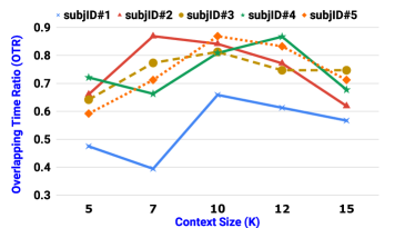
First we determine the optimal context size used in the sentence classifier described in Section IV-B. For finding the optimal context size we make a holistic evaluation of the segmented topics and compare the results with the ground truth. The context size $K$ should be such that the neighbourhood information is sufficient enough to predict accurate segment boundary as well as takes minimal time to train the model. Higher value of $K$ captures some unnecessary context while too lowering this value may not properly capture the original context. We optimize the value of $K$ by measuring the segmentation accuracy using OTR metric on the dataset. Figure  13 shows the experimental result on different values of $K$. After experiment we take the value of $K$ (number of sentences in each context) as $10$ with $20$ words in each sentence.

Figure 13: Context Size vs OTR Score

To determine the threshold value of topic duration, we perform some experiments that will make some comparative analysis between structural segmentation and semantic segmentation based on topic duration. From the $66$ lecture videos on software engineering domain we get $225$ topics. We divide these topics into two category according to their duration. We find $164$ topics has duration less than $15$ minutes while $91$ topics have duration more than $15$ minutes. We measure the segmentation accuracy on these two group of topics and find the results as shown in the Table VI.

The reason of this discrepancy between two approach for long duration topic is, structural analysis primarily focuses on the local context on a text block, more specifically it produce best result for particular context size. If the lecture video duration is greater than the context size, the underlined model is not able to capture the global context. If the topic duration is smaller than the context size the model ignores some important context. Use of knowledge graph and semantic analysis alleviates this problem and perform better for the large length topic segments. For more illustration, we have divided these $255$ topics obtained from $65$ videos into four different category based on their duration. the duration categories with the corresponding number of topics are given below.

123 topic with duration 10 minutes to 15 minutes.

123 topic with duration 15 minutes to 20 minutes.

123 topic with duration 20 minutes to 25 minutes.

123 topic with duration more than 25 minutes.

Figure 14: Comparison between structural analysis and semantic analysis on large length topics.

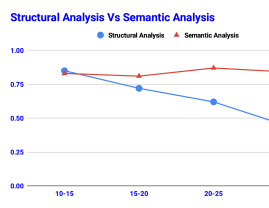
We measure group wise segmentation accuracy of two different algorithms proposed by us and Figure 14 shows the comparative results. It is clear from the figure that as the segment duration increases accuracy of structural analysis based method decreases. While on the other hand, semantic analysis based approach produces steady performance irrespective of the topic size.

IX Conclusion

In this work we detect the topic boundaries of long MOOC lecture videos. These topics can be used for indexing purpose on which user can perform topic search that reduce user time of locating and browsing a topic inside a lecture video. For doing this we use a state-of-the art language model to capture boundary information. Also we leverage the inherent knowledge present inside a doamin knowledge graph for fine tuning the segmentation result and accurately detecting the topics of larger time duration. In this work we have used LSTM with attention layer as the language model and BERT for capturing the overall semantics of the text corpora. In future we have a plan to use transformaer instead of LSTM and use domain specific BERT model for getting better segmentation result.

References

- [1] “National program on technology enhanced learning,” 2019. [Online]. Available: https://nptel.ac.in/
- [2] A. M. Kaplan and M. Haenlein, “Higher education and the digital revolution: About moocs, spocs, social media, and the cookie monster,” Business Horizons, vol. 59, no. 4, pp. 441–450, 2016.
- [3] M. Lin, J. F. Nunamaker Jr, M. Chau, and H. Chen, “Segmentation of lecture videos based on text: a method combining multiple linguistic features,” in null. IEEE, 2004, p. 10003c.
- [4] T. Mikolov, K. Chen, G. Corrado, and J. Dean, “Efficient estimation of word representations in vector space,” arXiv preprint arXiv:1301.3781, 2013.
- [5] R. R. Shah, Y. Yu, A. D. Shaikh, and R. Zimmermann, “Trace: Linguistic-based approach for automatic lecture video segmentation leveraging wikipedia texts,” in Multimedia (ISM), 2015 IEEE International Symposium on. IEEE, 2015, pp. 217–220.
- [6] S. Repp, A. Grob, and C. Meinel, “Browsing within lecture videos based on the chain index of speech transcription,” IEEE Transactions on learning technologies, vol. 1, no. 3, pp. 145–156, 2008.
- [7] H. Chen, M. Cooper, D. Joshi, and B. Girod, “Multi-modal language models for lecture video retrieval,” in Proceedings of the 22nd ACM international conference on Multimedia. ACM, 2014, pp. 1081–1084.
- [8] R. R. Shah, Y. Yu, A. D. Shaikh, S. Tang, and R. Zimmermann, “Atlas: automatic temporal segmentation and annotation of lecture videos based on modelling transition time,” in Proceedings of the 22nd ACM international conference on Multimedia. ACM, 2014, pp. 209–212.
- [9] D. Galanopoulos and V. Mezaris, “Temporal lecture video fragmentation using word embeddings,” in International Conference on Multimedia Modeling. Springer, 2019, pp. 254–265.
- [10] H. Yang, M. Siebert, P. Luhne, H. Sack, and C. Meinel, “Automatic lecture video indexing using video ocr technology,” in Multimedia (ISM), 2011 IEEE International Symposium on. IEEE, 2011, pp. 111–116.
- [11] X. Che, H. Yang, and C. Meinel, “Lecture video segmentation by automatically analyzing the synchronized slides,” in Proceedings of the 21st ACM international conference on Multimedia. ACM, 2013, pp. 345–348.
- [12] H. J. Jeong, T.-E. Kim, and M. H. Kim, “An accurate lecture video segmentation method by using sift and adaptive threshold,” in Proceedings of the 10th International Conference on Advances in Mobile Computing & Multimedia. ACM, 2012, pp. 285–288.
- [13] Y. Goldberg, “Neural network methods for natural language processing,” Synthesis Lectures on Human Language Technologies, vol. 10, no. 1, pp. 1–309, 2017.
- [14] I. Goodfellow, Y. Bengio, A. Courville, and Y. Bengio, Deep learning. MIT press Cambridge, 2016, vol. 1, no. 2.
- [15] M. A. Hearst, “Texttiling: Segmenting text into multi-paragraph subtopic passages,” Computational linguistics, vol. 23, no. 1, pp. 33–64, 1997.
- [16] S. Basu, Y. Yu, V. K. Singh, and R. Zimmermann, “Videopedia: Lecture video recommendation for educational blogs using topic modeling,” in International Conference on Multimedia Modeling. Springer, 2016, pp. 238–250.
- [17] E. Baidya and S. Goel, “Lecturekhoj: automatic tagging and semantic segmentation of online lecture videos,” in 2014 Seventh international conference on contemporary computing (IC3). IEEE, 2014, pp. 37–43.
- [18] M. Eberts, A. Ulges, and U. Schwanecke, “Amigo-automatic indexing of lecture footage,” in 2015 13th International Conference on Document Analysis and Recognition (ICDAR). IEEE, 2015, pp. 1206–1210.
- [19] D. Ma, X. Zhang, X. Ouyang, and G. Agam, “Lecture vdeo indexing using boosted margin maximizing neural networks,” in 2017 16th IEEE International Conference on Machine Learning and Applications (ICMLA). IEEE, 2017, pp. 221–227.
- [20] D. Ma and G. Agam, “Lecture video segmentation and indexing,” in Document Recognition and Retrieval XIX, vol. 8297. International Society for Optics and Photonics, 2012, p. 82970V.
- [21] H. Yang and C. Meinel, “Content based lecture video retrieval using speech and video text information,” IEEE Transactions on Learning Technologies, vol. 1, no. 2, pp. 142–154, 2014.
- [22] A. Conneau, D. Kiela, H. Schwenk, L. Barrault, and A. Bordes, “Supervised learning of universal sentence representations from natural language inference data,” arXiv preprint arXiv:1705.02364, 2017.
- [23] S. R. Bowman, G. Angeli, C. Potts, and C. D. Manning, “A large annotated corpus for learning natural language inference,” arXiv preprint arXiv:1508.05326, 2015.
- [24] P. Badjatiya, L. J. Kurisinkel, M. Gupta, and V. Varma, “Attention-based neural text segmentation,” in European Conference on Information Retrieval. Springer, 2018, pp. 180–193.
- [25] S. Hochreiter and J. Schmidhuber, “Long short-term memory,” Neural computation, vol. 9, no. 8, pp. 1735–1780, 1997.
- [26] “Wikipedia,” 2019. [Online]. Available: https://en.wikipedia.org/
- [27] M. D. Zeiler, “Adadelta: an adaptive learning rate method,” arXiv preprint arXiv:1212.5701, 2012.
- [28] A. Akbik, T. Bergmann, D. Blythe, K. Rasul, S. Schweter, and R. Vollgraf, “Flair: An easy-to-use framework for state-of-the-art nlp,” in Proceedings of the 2019 Conference of the North American Chapter of the Association for Computational Linguistics (Demonstrations), 2019, pp. 54–59.
- [29] J. Devlin, M.-W. Chang, K. Lee, and K. Toutanova, “Bert: Pre-training of deep bidirectional transformers for language understanding,” arXiv preprint arXiv:1810.04805, 2018.
- [30] B. Epshtein, E. Ofek, and Y. Wexler, “Detecting text in natural scenes with stroke width transform,” in Computer Vision and Pattern Recognition (CVPR), 2010 IEEE Conference on. IEEE, 2010, pp. 2963–2970.
- [31] “Tesseract open source ocr, engine,” 2019. [Online]. Available: https://github.com/tesseract-ocr/
- [32] M. Kusner, Y. Sun, N. Kolkin, and K. Weinberger, “From word embeddings to document distances,” in International Conference on Machine Learning, 2015, pp. 957–966.
- [33] P. Jaccard, “Nouvelles recherches sur la distribution florale,” Bull. Soc. Vaud. Sci. Nat., vol. 44, pp. 223–270, 1908.
- [34] D. Beeferman, A. Berger, and J. Lafferty, “Text segmentation using exponential models,” arXiv preprint cmp-lg/9706016, 1997.
- [35] L. Pevzner and M. A. Hearst, “A critique and improvement of an evaluation metric for text segmentation,” Computational Linguistics, vol. 28, no. 1, pp. 19–36, 2002.