Modelling General Properties of Nouns
by Selectively Averaging Contextualised Embeddings

Abstract

While the success of pre-trained language models has largely eliminated the need for high-quality static word vectors in many NLP applications, such vectors continue to play an important role in tasks where words need to be modelled in the absence of linguistic context. In this paper, we explore how the contextualised embeddings predicted by BERT can be used to produce high-quality word vectors for such domains, in particular related to knowledge base completion, where our focus is on capturing the semantic properties of nouns. We find that a simple strategy of averaging the contextualised embeddings of masked word mentions leads to vectors that outperform the static word vectors learned by BERT, as well as those from standard word embedding models, in property induction tasks. We notice in particular that masking target words is critical to achieve this strong performance, as the resulting vectors focus less on idiosyncratic properties and more on general semantic properties. Inspired by this view, we propose a filtering strategy which is aimed at removing the most idiosyncratic mention vectors, allowing us to obtain further performance gains in property induction.

1 Introduction

The success of contextualised language models (LMs), such as BERT Devlin et al. (2019), has led to a paradigm shift in Natural Language Processing (NLP). A key feature of such models is that they produce contextualised word vectors, i.e. vectors that represent the meaning of words in the context of a particular sentence. While the shift away from standard word embeddings has benefited an impressively wide range of NLP tasks, many other tasks still crucially rely on static representations of word meaning. For instance, in information retrieval, query terms often need to be modelled without any other context, and word vectors are commonly used for this purpose Onal et al. (2018). In zero shot learning, word vectors are used to obtain category embeddings Socher et al. (2013); Ma et al. (2016). Word vectors are also used in topic models Das et al. (2015). In the context of the Semantic Web, word vectors have been used for ontology alignment Kolyvakis et al. (2018), concept invention Vimercati et al. (2019) and ontology completion Li et al. (2019). The word vectors learned by standard word embedding models, such as Skip-gram Mikolov et al. (2013) and GloVe Pennington et al. (2014), essentially summarise the contexts in which each word occurs. However, these contexts are modelled in a shallow way, capturing only the number of co-occurrences between target words and individual context words. The question we address in this paper is whether the more sophisticated context encodings that are produced by LMs can be used to obtain higher-quality word vectors. Motivated by the aforementioned applications, we focus in particular embeddings that capture the semantic properties of nouns.

To obtain static word vectors from a contextualised language model, we can sample sentences in which a given word $w$ occurs, obtain a contextualised vector representation of $w$ from these sentences, and finally average these vectors Bommasani et al. (2020); Vulic et al. (2020). In this paper, we aim to improve on this strategy. First, when obtaining a contextualised representation of the target word, we replace that target word by the [MASK] token. This has the advantage that words which consist of multiple word-pieces can be modelled in a natural way. More fundamentally, our hypothesis is that this will lead to representations that are more focused on the semantic properties of the given word. In particular, because the target word is masked, the resulting vector specifically captures what that sentence reveals about the word. A bag of masked sentences can thus be viewed as a bag of properties. To illustrate this, consider the Wikipedia sentences in Table 1, where occurrences of the word bananas were masked. From BERT’s top predictions for the missing word, we can see that these sentences indeed reveal different properties of bananas, e.g. being edible, a dessert ingredient and a type of fruit.

Masked sentence	BERT predictions
aaa are cultivated by both small farmers and large land holders.	they, these, crops, fields, potatoes, gardens, vegetables, most, vines, trees
Banoffee pie is an English dessert pie made from aaa, cream and toffee …	cheese, sugar, butter, apples, eggs, milk, chocolate, honey, apple, egg
aaa are a popular fruit consumed worldwide with a yearly production of over …	they, bananas, citrus, apples, grapes, these, fruits, potatoes, berries, nuts

Table 1: Top predictions from BERT-large-uncased for sentences.

This view of masked sentences as encoding properties suggests another improvement over plain averaging of contextualised vectors. Since some properties are intuitively more important than others, we should be able to improve the final representations by averaging only a particular selection of the contextualised vectors. Consider the following Wikipedia sentence: Banana equivalent dose (BED) is an informal measurement of ionizing radiation exposure. By masking the word “banana”, we can obtain a contextualised vector, but this vector would not capture any of the properties that we would normally associate with bananas. The crucial difference with the sentences from Table 1 is that the latter capture general properties, i.e. properties that apply to more than one concept, whereas the sentence above captures an idiosyncratic property, i.e. a property that only applies to a particular word. In the aforementioned application domains, static word vectors are essentially used to capture the commonalities between given sets of words (e.g. between training and test categories in zero shot learning). Word vectors should thus primarily capture the general properties of nouns. Inspired by this view, we propose a simple strategy for identifying contextualised vectors that are likely to capture idiosyncratic properties. When computing the vector representation of a given noun, we then simply omit these mention vectors, and compute the average of the remaining ones.

2 Related Work

Several authors have analysed the extent to which pre-trained LMs capture semantic knowledge. For instance, Forbes et al. Forbes et al. (2019) focused on predicting the properties of concepts (i.e. nouns), as well as their affordances (i.e. how they can be used). Weir et al. Weir et al. (2020) considered the following problem: given a sentence that specifies the properties of a given concept, can LMs be used to predict the concept? For instance, given the input “A [MASK] is tasty, is eaten, is made of sugar, is made of flour, and is made of eggs”, the aim is to predict cake. Some previous work has already explored the idea of using the contextualised word vectors predicted by neural LMs for modelling word meaning. For instance, Amrami and Goldberg Amrami and Goldberg (2019) obtain the set of contextualised vectors predicted by BERT, for different mentions of the same word, and then cluster these vectors to perform word sense induction. Mickus et al. Mickus et al. (2019) analyse the distribution of contextualised word vectors, finding that the vectors corresponding to the same word type are largely clustered together. The distribution of contextualised word vectors is also studied by Ethayarajh Ethayarajh (2019), who furthermore explores the idea of learning static word vectors by taking the first principal component of the contextualised vectors of a given word (which has a similar effect as taking their average). They find that the vectors obtained from the earlier layers of BERT (and other LMs) perform better in word similarity tasks than the later layers. In contrast, Bommasani et al. Bommasani et al. (2020) found that the optimal layer depends on the number of sampled mentions, with later layers performing better with a large number of mentions. Rather than fixing a single layer, Vulic et al. Vulic et al. (2020) advocated averaging representations from several layers.

3 Encoding Words with Mention Vectors

In this section we describe our strategy for obtaining static word vectors from BERT. First, we provide some background on the BERT model and we explain how we use BERT to obtain mention vectors for a given word. Finally, we also introduce our proposed filtering strategy.

Background and Notation

BERT represents text fragments as sequences of tokens. Frequent words are represented as a single token, whereas less common words are represented as sequences of sub-word tokens, called word-pieces. Given an input sentence $S=t_{1}...t_{k}$, BERT predicts a contextualised vector $\phi_{i}(S)$ for each token $t_{i}$. Together with this mapping $\phi$, which takes the form of a deep transformer model, BERT learns a static vector $\mathbf{t}_{\textsc{static}}$ for each word-piece $t$ in its vocabulary $V_{\textsc{BERT}}$. During training, some tokens are replaced by a special token [MASK]. If this is the case for the i^th token of the sentence $S$, $\phi_{i}(S)$ encodes a probability distribution over word-pieces, corresponding to BERT’s prediction of which token from the original sentence was masked.

Obtaining Mention Vectors

Let $W$ be the set of nouns for which we want to learn a vector representation. For each $w\in W$, we randomly sample $N$ mentions of $w$ from a given corpus. From each of the corresponding sentences, we obtain a vector by masking the occurrence of $w$ and taking the contextualised vector predicted by BERT for the position of this [MASK] token. We will refer to this vector as a mention vector. For $w\in W$, we write $\mu(w)$ for the set of all mention vectors that are obtained for $w$. A key design choice in our approach is that we mask the occurrences of $w$ for obtaining the mention vectors. This has two important advantages. First, it allows us to specifically capture what each sentence reveals about $w$. In particular, $\mathbf{w}_{\textsc{Avg}}$ reflects the properties of $w$ that can be inferred from typical sentences mentioning this word, rather than the properties that best discriminate $w$ from other words. The result is that the vectors $\mathbf{w}_{\textsc{Avg}}$ are qualitatively different from the vectors that are obtained by standard word embedding models, as we will see in the experiments in Section 4. Second, since we replace $w$ by a single [MASK] token, we always obtain a single vector, even if $w$ corresponds to multiple word-pieces. In contrast, without masking, the predictions for the different word-pieces from the same word have to be aggregated in some way.

Filtering Idiosyncratic Mention Vectors

Our aim is to learn vector representations that reflect the semantic properties of nouns. One possible strategy is to compute the average $\mathbf{w}_{\textsc{Avg}}$ of the mention vectors in $\mu(w)$. However, some of these mention vectors are likely to capture idiosyncratic properties. Our hypothesis is that including such mention vectors degrades the quality of the word representations. To test this hypothesis, we introduce a strategy for identifying idiosyncratic mention vectors. For each mention vector $\mathbf{m}\in\mu(w)$, we compute its $k$ nearest neighbours, in terms of cosine similarity, among the set of all mention vectors that were obtained for the vocabulary $W$, i.e. the set $\bigcup_{v\in W}\mu(v)$. If all these nearest neighbours belong to $\mu(w)$ then we assume that $\mathbf{m}$ is too idiosyncratic and should be removed. Indeed, this suggests that the corresponding sentence expresses a property that only applies to $w$. We then represent $w$ as the average $\mathbf{w}^{*}$ of all remaining mention vectors, i.e. all mention vectors from $\mu(w)$ that were not found to be idiosyncratic.

4 Evaluation

Our aim is to analyse (i) the impact of masking on the averaged mention vectors and (ii) the effectiveness of the proposed filtering strategy. In Section 4.1, we focus on the task of predicting semantic properties of words, while Section 4.2 discusses word similarity. In Section 4.3, we then evaluate the mention vectors on the downstream task of ontology completion. Section 4.4 presents some qualitative analysis.

Vector Representations. We use two standard word embedding models for comparison: Skip-gram (SG) Mikolov et al. (2013) and GloVe Pennington et al. (2014). In both cases, we used 300-dimensional embeddings that were trained on the English Wikipedia. For the contexualised vectors, we rely on two pre-trained language models: BERT-large-uncased Devlin et al. (2019) and RoBERTa-large Liu et al. (2019). We compare a number of different strategies for obtaining word vectors from these language models. First, we use the input vectors $\mathbf{t}_{\textsc{static}}$ (Input). For words which are not in the word-piece vocabulary, following common practice Bommasani et al. (2020); Vulic et al. (2020), we average the input embeddings of their words-pieces. As the corpus for extracting mention vectors, we use the May 2016 dump of the English Wikipedia. We considered sentences of length at most 64 words to compute mention vectors, as we found that longer sentences were often the result of sentence segmentation errors. In the experiments, we only consider nouns that are mentioned in at least 10 such sentences. For nouns that occur more than 500 times, we use a random sample of 500 mentions.

We compare two versions of the averaged mention vectors (with masking): the average of all mention vectors (AVG${}_{\textit{last}}$) and the average of those that remain after applying the filtering strategy (AVG${}_{\textit{filt}}$). As a baseline filtering strategy, we also show results for a variant where mention vectors were filtered based on their distance from their mean (AVG${}_{\textit{outl}}$). For this baseline, we remove a fixed percentage of the mention vectors, where this percentage is tuned as a hyper-parameter.

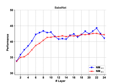
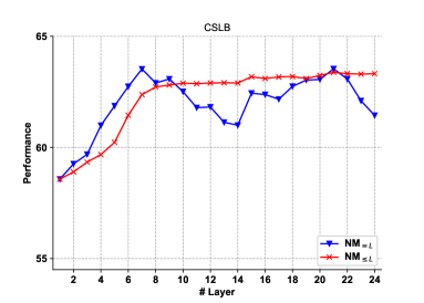
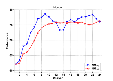
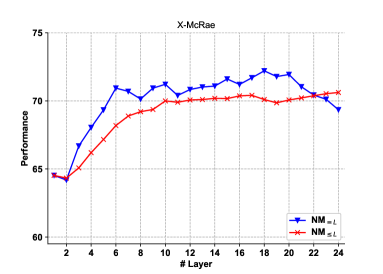
We also include several variants in which mention vectors are obtained without masking. For words that consist of more than one word-piece, we average the contextualised word-piece vectors. We consider the counterparts of AVG${}_{\textit{last}}$, AVG${}_{\textit{filt}}$ and AVG${}_{\textit{outl}}$, which we will refer to as NM${}_{\textit{last}}$, NM${}_{\textit{filt}}$ and NM${}_{\textit{outl}}$ respectively. Note that these strategies only look at the final layer. Previous work has found that earlier layers sometimes yield better results on lexical semantics benchmarks Bommasani et al. (2020). For this reason, we also include a method that chooses the best layer for a given task based on the tuning split, and then uses the representations at that layer (NM_=L). Finally, Vulic et al. Vulic et al. (2020) suggested to take the average of the first $\ell$ layers. We also show results for this approach, where the number of layers $\ell$ is again selected for each task based on tuning data (NM_≤L).

Dataset	Type	Nouns	Classes
X-McRae	Commonsense	513	50
CSLB	Commonsense	635	395
Morrow	Taxonomic	888	13
WN supersenses	Taxonomic	18200	25
BN domains	Topical	12477	28

Table 2: Overview of the lexical classification datasets.

4.1 Modelling Semantic Properties

Datasets. We consider lexical classification benchmarks involving three types of semantic properties: commonsense properties (e.g. table is made of wood), taxonomic properties (e.g. table is a type of furniture) and topics or domains (e.g. football is related to sports). In particular, we used two datasets which are focused on commonsense properties (e.g. being dangerous, edible, made of metal). First, we used the extension of the McRae feature norms dataset McRae et al. (2005) that was introduced in Forbes et al. (2019) (X-McRae). In contrast to the original McRae feature norms, this dataset contains genuine positive and negative examples for all properties. We considered all properties for which at least 10 positive examples are available in the dataset, resulting in a total of 50 classes. Second, we considered CSLB Concept Property Norms, which is similar in spirit to the McRae feature norms dataset. For this dataset, we again limited our analysis to properties with at least 10 positive examples. We furthermore consider two datasets that are focused on taxonomic properties. First, we use the dataset that was introduced by Morrow and Duffy Morrow and Duffy (2005), which lists instances of 13 everyday categories (e.g. animals, fruits, furniture, instruments). Second, we used the WordNet supersenses, which organises nouns into broad categories, such as person, animal and plant Ciaramita and Johnson (2003). As a final dataset, we used the BabelNet domains Camacho-Collados and Navigli (2017), which are domain labels of lexical entities, such as music, language, and medicine. Table 2 provides some statistics about the considered datasets.

	X-McRae		CSLB		Morrow		WordNet		BabelNet
	MAP	F1	MAP	F1	MAP	F1	MAP	F1	MAP	F1
GloVe	47.7	40.1	43.8	31.8	54.4	50.6	42.4	39.4	33.9	31.8
SG	57.7	49.3	53.3	39.9	76.6	61.2	53.2	53.2	45.5	39.6
Input	69.1	59.2	56.5	41.4	54.7	45.9	33.3	35.9	29.3	31.8
NM${}_{\textit{last}}$	70.8	61.3	60.8	45.9	73.0	56.2	45.6	43.5	38.7	38.8
NM${}_{\textit{outl}}$	68.5	58.6	62.1	47.8	74.3	68.2	41.9	43.2	39.8	39.2
NM${}_{\textit{filt}}$	45.0	42.2	49.0	36.0	62.7	48.8	31.9	33.6	31.2	32.8
NM=L	70.4	60.4	62.7	49.9	78.5	58.5	46.7	44.6	43.4	39.3
NM≤L	70.6	60.9	63.3	48.8	76.4	62.9	46.6	44.8	42.6	40.1
AVG${}_{\textit{last}}$	72.5	62.8	59.3	46.5	77.5	67.3	66.5	60.9	57.4	52.1
AVG${}_{\textit{outl}}$	68.1	61.1	61.3	49.9	77.2	66.5	50.9	50.6	42.3	41.8
AVG${}_{\textit{filt}}$	73.0	64.1	64.4	50.9	81.7	70.1	67.8	61.2	57.9	52.5

Table 3: Results ($\%$) for BERT-large-uncased on the lexical classification tasks, in terms of MAP and F1 scores ($\%$).

	X-McRae		CSLB		Morrow		WordNet		BabelNet
	MAP	F1	MAP	F1	MAP	F1	MAP	F1	MAP	F1
GloVe	47.7	40.1	43.8	31.8	54.4	50.6	42.4	39.4	33.9	31.8
SG	57.7	49.3	53.3	39.9	76.6	61.2	53.2	53.2	45.5	39.6
Input	39.9	34.0	36.6	25.7	31.5	32.5	45.6	43.8	33.0	30.8
NM${}_{\textit{last}}$	65.2	54.4	57.2	42.9	75.2	62.5	53.0	50.9	41.2	40.5
NM${}_{\textit{outl}}$	66.1	53.7	58.1	44.4	78.5	68.9	53.8	51.6	42.4	41.8
NM${}_{\textit{filt}}$	37.8	33.0	40.7	29.3	57.5	43.6	39.4	41.1	35.6	36.3
NM=L	65.2	55.9	60.5	45.6	79.0	67.5	53.0	50.9	43.4	40.3
NM≤L	63.9	53.5	58.9	44.2	77.9	67.5	51.3	50.2	43.1	39.3
AVG${}_{\textit{last}}$	72.1	63.9	54.6	44.8	72.4	57.8	62.3	56.5	53.2	49.3
AVG${}_{\textit{outl}}$	67.8	60.0	59.1	47.8	77.7	66.5	50.9	50.6	40.9	41.2
AVG${}_{\textit{filt}}$	74.3	64.8	62.2	51.4	81.8	73.5	63.9	58.5	54.6	50.9

Table 4: Results ($\%$) for RoBERTa-large on the lexical classification tasks, in terms of MAP and F1 scores ($\%$).

	SemEval	SimLex	WordSim
GloVe	70.5	43.7	78.2
SG	71.1	40.9	79.3
Input	63.3	50.9	72.9
NM${}_{\textit{last}}$	66.5	58.7	70.9
NM≤L ($\ell=24$)	78.4	57.8	82.6
NM${}_{\textit{filt}}$	51.6	43.4	50.0
AVG${}_{\textit{last}}$	55.4	41.0	60.9
AVG${}_{\textit{filt}}$ ($k=5$)	64.0	42.6	67.6
NM≤L ($\ell=24$) + SG	76.5	51	83.5
AVG${}_{\textit{last}}$ + SG	70.5	43.1	75.7
AVG${}_{\textit{filt}}$ ($k=5$) + SG	75.2	43.2	78.9

Table 5: Word similarity results for BERT (Spearman correlation).

Figure 1: Results of NM_=L and NM_≤L per layer for WordNet supersenses with BERT.

Top quartile gold pairs ranked in bottom quartile
SimLex	(right, justice), (adult, guardian), (bird, turkey), (bubble, suds), (crowd, bunch), (flower, violet), (alcohol, cocktail), (evening, dusk), (wisdom, intelligence), (marijuana, herb), (intelligence, logic), (sofa, chair), (communication, language), (violin, instrument), (politician, president), (rabbi, minister)
SemEval	(cell, lock-up), (can, bottle), (coca-cola, coke), (obama, clinton), (renaissance, renascence), (amazon, forest), (english, american), (mercury, jupiter), (mercedes, opel), (plato, aristotle), (orion, constellation), (playstation, wii), (nike, adidas), (backgammon, go), (kfc, mcdonald’s), (guardian, times), (paint, photoshop), (jpeg, pdf), (bible, gospel), (gauss, scientist), (chart, graph)
WordSim	(mexico, brazil), (dollar, buck), (harvard, yale), (cell, phone)
Bottom quartile gold pairs ranked in top quartile
SimLex	(meat, bread), (winter, summer), (dog, cat), (floor, ceiling), (south, north), (absence, presence), (chocolate, pie), (bread, cheese), (river, valley), (sunset, sunrise), (dog, horse), (cat, rabbit), (lawyer, banker), (wife, husband), (bottom, top), (mouse, cat), (sun, sky)
SemEval	(gravity, meteor), (wood, blanket)
WordSim	(lad, wizard)

Table 6: Analysis of the similarity results for AVG${}_{\textit{filt}}$.

Experimental Setup. For all datasets, we train a binary linear SVM classifier for each of the associated classes. In the case of X-McRae, we used the standard training and test splits that were provided as part of this dataset. As no validation set was provided, we reserved 20% of the training split for hyper-parameter tuning. For the remaining four datasets, we randomly split the positive examples, for each class, into 60% for training, 20% for tuning and 20% for testing. Since these datasets do not provide explicit negative examples, for the test set we randomly select words from the other classes as negative examples (excluding words that also belong to the target category). The number of negative test examples was chosen as 5 times the number of positive examples. For the training and tuning sets, we randomly select nouns from the BERT vocabulary as negative examples. The number of negative examples for training was set as twice the number of positive examples. We report results of the SVM classifiers in terms of F1 score and Mean Average Precision (MAP). The latter treats the problem as a ranking task rather than a classification task, which is motivated by the fact that finding the precise classification boundary is difficult without true negative examples. Details about hyper-parameter tuning can be found in the supplementary materials.

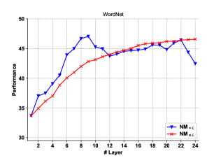
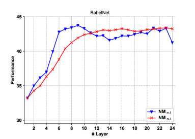
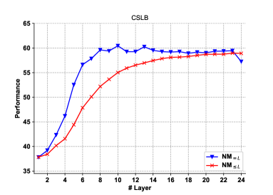
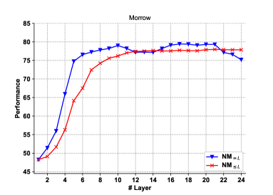
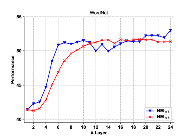
Results. The results are shown in Table 3 for BERT and in Table 4 for RoBERTa. In all cases, we find that the best results are obtained for the averaged mention vectors with our proposed filtering strategy (AVG${}_{\textit{filt}}$). The baseline filtering strategy (AVG${}_{\textit{outl}}$) is clearly not competitive, leading to worse results than AVG${}_{\textit{last}}$ in most cases. Another clear observation is that our proposed filtering strategy is clearly unsuitable for the NM vectors. This is because without masking, the mention vectors are clustered per word type Mickus et al. (2019), hence the filtering strategy simply removes the majority of the mention vectors in this case; e.g. for X-McRae, without masking 83.1% of the BERT mention vectors are filtered, compared to 39.7% with masking. Overall, strategies with masking outperform those without masking, often substantially. Among the strategies without masking, NM_=L and NM_≤L perform best, confirming the finding from earlier work that the last layer is not always optimal Bommasani et al. (2020), although in contrast to Vulic et al. Vulic et al. (2020) we do not find that NM_≤L clearly outperforms NM_=L. For NM_≤L we find that $\ell=24$ is chosen for most of the cases, whereas for NM_=L layers 8-10 are often best. Figure 1 shows the performance per layer for WordNet supersenses. Layer-wise results for all datasets are provided in the supplementary materials.

4.2 Word Similarity

We now consider word similarity benchmarks, where the task consists in ranking word pairs based on their degree of similarity. This ranking is then compared with a gold standard obtained from human judgements. We consider three standard word similarity datasets for nouns: the similarity portion of WordSim Agirre et al. (2009), the noun subset of SimLex Hill et al. (2015) and SemEval-17 Camacho-Collados et al. (2017). Many word similarity datasets, such as MEN Bruni et al. (2014), RG-65 Rubenstein and Goodenough (1965) or the full WordSim-353 Finkelstein et al. (2002), measure relatedness (or degree of association). In contrast, the datasets that we consider here all mainly focus on similarity. In particular, SimLex does not consider relatedness at all in the similarity scale, while SemEval and WordSim only consider relatedness in the lower grades of their similarity scales.

Table 5 shows the results of the word similarity experiments (for BERT). For SimLex, which is least affected by relatedness, all BERT based representations outperform SG, but the masking based strategies underperform GloVe. For the two other datasets, the masking based strategies underperform the SG and GloVe baselines. In all cases, the filtering strategy AVG${}_{\textit{filt}}$ improves the results of AVG${}_{\textit{last}}$, but the best results are consistently found without masking. To analyse the complementarity of the representations, we also experiment with strategies where two different representations are concatenated (after normalising the vectors). For AVG${}_{\textit{filt}}$ this considerably improves the results, which shows that SG and AVG${}_{\textit{filt}}$ capture complementary aspects of similarity. To better understand the reasons for the under-performance of AVG${}_{\textit{filt}}$, Table 6 shows all pairs that are within the top quartile of most similar pairs according to the gold ratings while being in the bottom quartile according to the AVG${}_{\textit{filt}}$ vector similarity, and vice versa. As can be seen, the pairs with high gold ratings but low vector similarity include several hypernym pairs (shown in blue) and named entities (shown in green). Conversely, the pairs with low gold ratings but high vector similarity include mostly co-hyponyms and antonyms (shown in red).

	Wine	Econ	Olym	Tran	SUMO
SG	13.8	13.5	8.3	7.2	33.4
Input	22.2	14.2	12.1	9.4	36.5
NM${}_{\textit{last}}$	18.5	12.5	16.2	12.3	38.9
NM${}_{\textit{filt}}$	20.3	15.6	13.3	11.2	35.4
AVG${}_{\textit{last}}$	23.0	20.0	16.9	11.5	41.4
AVG${}_{\textit{filt}}$	24.5	24.3	22.9	13.0	46.4

Table 7: Results ($\%$ F1) for ontology completion for BERT.

	saint
NM${}_{\textit{last}}$	st, sainthood, saintliness, stob, strontianite, sanctuary
AVG${}_{\textit{last}}$	st, pope, monsieur, prince, martyr, sage, antipope
AVG${}_{\textit{filt}}$	martyr, bishop, archangel, sage, patriarch, deacon
	emeritus
NM${}_{\textit{last}}$	adviser, incumbent, appointment, retirement, honorarium
AVG${}_{\textit{last}}$	dean, visiting, hod, excellency, chair, professor, assistant
AVG${}_{\textit{filt}}$	fellow, laureate, excellency, provost, principal, hod
	rent
NM${}_{\textit{last}}$	rentier, rental, lease, tenant, landlord, renter, leasehold
AVG${}_{\textit{last}}$	lease, rental, royalty, mortgage, scrip, wage, cash
AVG${}_{\textit{filt}}$	lease, mortgage, purchase, loan, expense, royalty, debt
	austrian
NM${}_{\textit{last}}$	austria, vienna, archduke, wiener, innsbruck, graz
AVG${}_{\textit{last}}$	slovak, czech, dutch, hungarian, brazilian, russian
AVG${}_{\textit{filt}}$	bavarian, dutch, slovak, belgian, russian, canadian

Table 8: Nearest neighbours for selected target words, in terms of cosine similarity, for the vocabulary from WordNet supersenses.

Target	Masked sentence
banana	Some countries produce statistics distinguishing between aaa and plantain production, but four of …
sardine	Traditional fisheries for anchovies and aaa also have operated in the Pacific, the Mediterranean, and …
lamb	Edison’s 1877 tinfoil recording of Mary Had a Little aaa, not preserved, has been called the first …
pineapple	In October 2000, the Big aaa, a tourist attraction on the Sunshine Coast, was used as a backdrop for …
salamander	The southern red-backed salamander (Plethodon serratus) is a species of aaa endemic to the United States.

Table 9: Examples of sentences whose corresponding mention vectors were filtered.

4.3 Ontology Completion

We now consider the downstream task of ontology completion. Given a set of ontological rules, the aim is to predict plausible missing rules Li et al. (2019); e.g. suppose the ontology contains the following rules:

$$\emph{Beer}(x) \rightarrow\emph{AlcoholicBeverage}(x)$$

$$\emph{Gin}(x) \rightarrow\emph{AlcoholicBeverage}(x)$$

As these rules have the same structure, they define a so-called rule template of the form

$$\star(x)\rightarrow\emph{AlcoholicBeverage}(x)$$

where $\star$ is a placeholder. Since substituting the placeholder by beer and gin makes the rule valid, and since wine shares most of the semantic properties that beer and gin have in common, intuitively it seems plausible that substituting $\star$ by wine should also produce a valid rule. To predict plausible rules in this way, Li et al. Li et al. (2019) used a graph-based representation of the rules. The nodes of this graph correspond to concepts (or predicates) while edges capture different types of interactions, derived from the rules. The predictions are made by a Graph Convolutional Network, where skip-gram embeddings of the concept names are used as the input node embeddings. In this experiment, we replace the skip-gram vectors by our averaged mention vectors and evaluate the resulting predictions on four well-known domain-specific ontologies (i.e. Wine, Economy, Olympics and Transport) and on the open-domain ontology SUMO. We used the pre-processed versions of these ontologies, and corresponding training and test splits, from Li et al. Li et al. (2019). As our focus is on evaluating the usefulness of the word vectors, we only generate templates for concepts whose names occur at least two times in Wikipedia. Furthermore, as the hyper-parameters of the GCN model are sensitive to the dimensionality of the input representations, we use Singular Value Decomposition to reduce the dimensionality of our vector representations from 1024 to 300, allowing us to keep the same hyper-parameter values as for the skip-gram vectors. For more details about the experimental methodology, we refer to Li et al. (2019). As this ontology completion model is computationally expensive, we restrict the set of baselines for this experiment, and show results for BERT only. The results are presented in Table 7, in terms of F1 confirm that the average mention vectors considerably outperform skip-gram vectors, and that the filtering strategy leads to further improvements.

4.4 Qualitative Analysis

Nearest neighbours. In Table 8, we show the nearest neighbours of four selected words. Some of the listed examples clearly illustrate how the proposed filtering step is successful in prioritizing general semantic properties. For instance, in the case of emeritus, filtering leads to lower ranks for university-related terms (e.g. dean and chair) and higher ranks for honorary positions (e.g. fellow and excellency). For rent, the filtering strategy increases the rank of concepts related to monetary transactions (e.g. “purchase” and “expense”). The effect of masking can be clearly seen in all examples, where strategies with masking (AVG${}_{\textit{last}}$ and AVG${}_{\textit{filt}}$) more consistently result in neighbours of the same kind. For example, for austrian, the masked variants consistently select demonyms, whereas the neighbours for NM${}_{\textit{last}}$ include various terms related to Austria. The example of saint also highlights how the need to average multiple word-piece vectors can introduce further noise, as some of the selected neighbours for NM${}_{\textit{last}}$ are included because they contain st as a word-piece, despite not being semantically related.

Figure 2: Plots of the mention vectors for sapling (left) and cockroach (right) from the Morrow dataset, showing the mention vectors which are removed by the filtering strategy (blue) and the corresponding static vector (red).

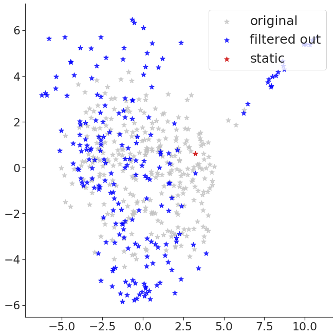
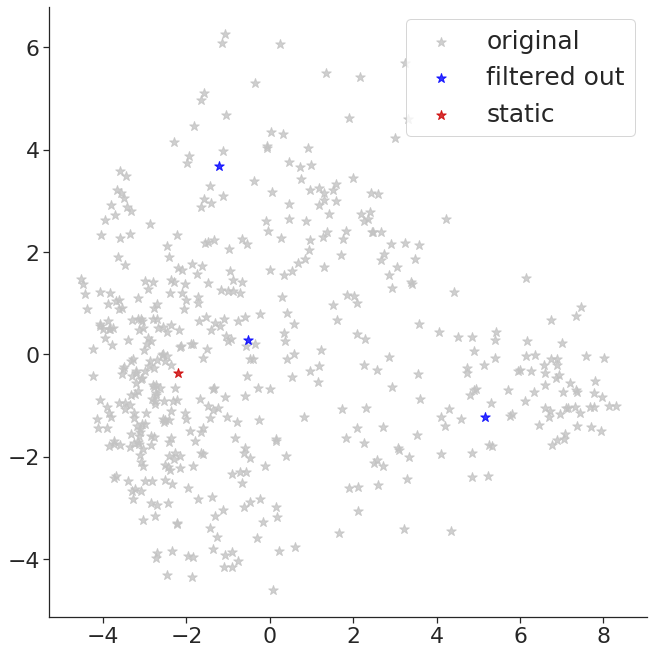
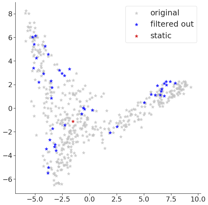
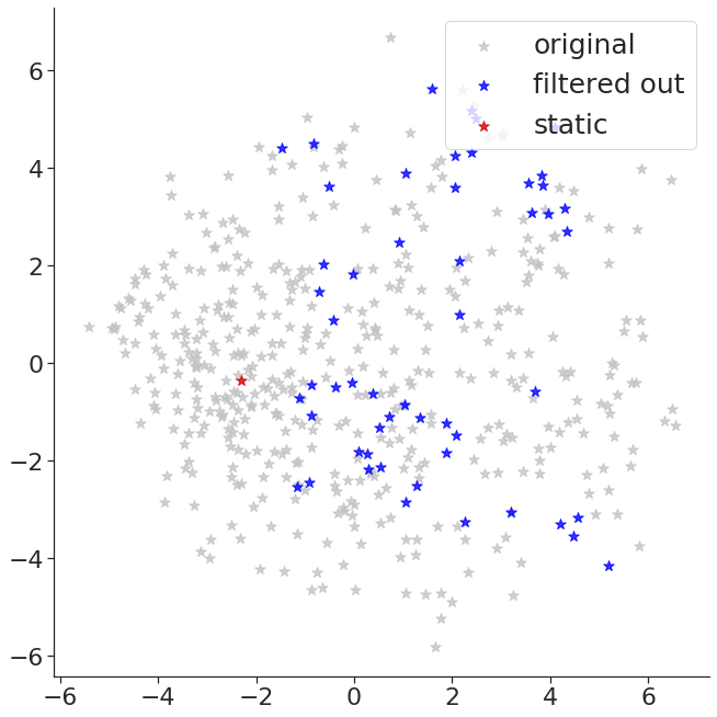
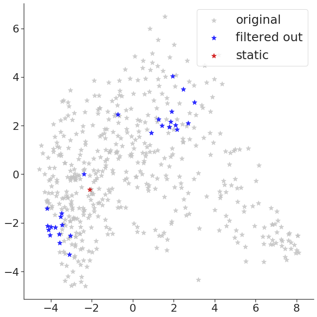
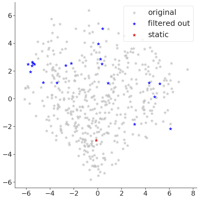
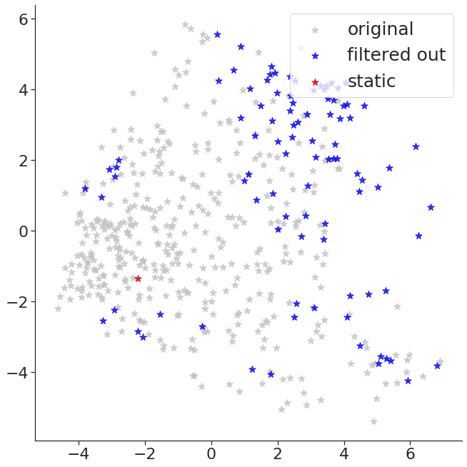
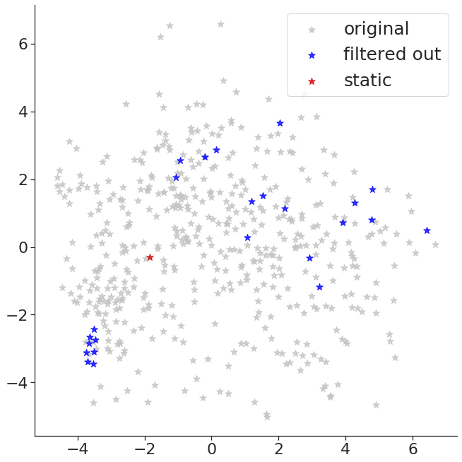
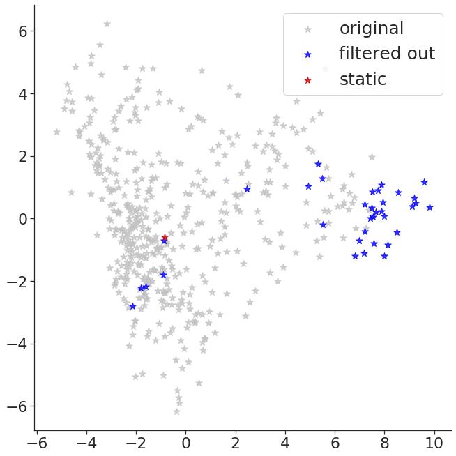
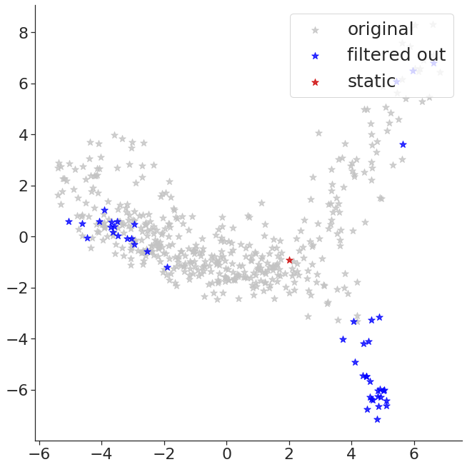
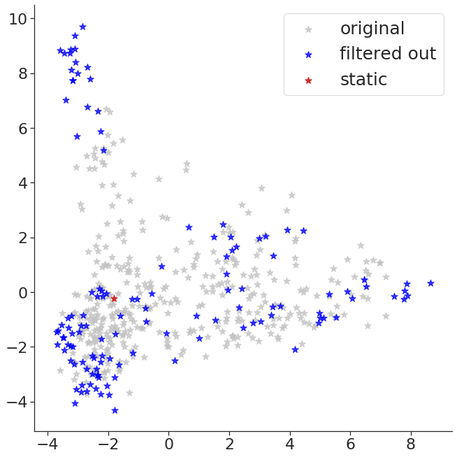
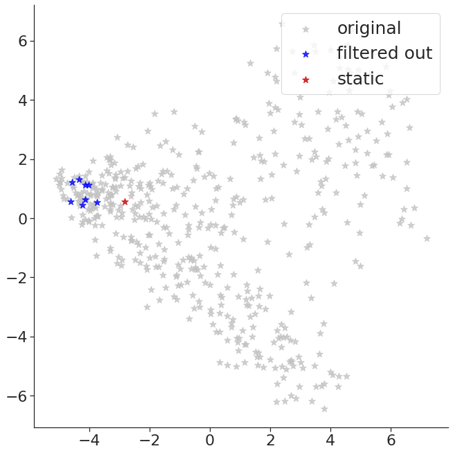
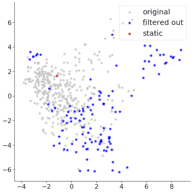
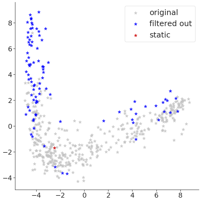
Examples of filtered mentions. Table 9 provides some examples of sentences whose resulting mention vector was filtered, for words from X-McRae. The sentence for banana asserts a highly idiosyncratic property, namely that the words banana and plantain are interchangeable in some contexts. The example for sardine is filtered because sardines and anchovies are often mentioned together. The examples for lamb and pineapple illustrate cases where the target word is used within the name of an entity, rather than on its own. Finally, as the example for salamander illustrates, highly idiosyncratic vectors can be obtained from sentences in which the target word is mentioned twice. To further illustrate the behaviour of the filtering strategy, Figure 2 depicts which mention vectors are filtered for two examples; further examples can be found in the supplementary materials. The figure shows that the strategy is adaptive, in the sense that a large number of mention vectors are filtered for some words, while only few vectors are filtered for other words. This clearly shows that our strategy is not simply removing outliers, which is in accordance with the poor performance of the AVG${}_{\textit{outl}}$ baseline.

5 Conclusion

We have analysed the potential of averaging the contextualised vectors predicted by BERT to obtain high-quality static word vectors. We found that the resulting vectors are qualitatively different depending on whether or not the target word is masked. When masking is used, the resulting vectors tend to represent words in terms of the general semantic properties they satisfy, which is useful in tasks where we have to identify words that are of the same kind, rather than merely related. We have also proposed a filtering strategy to obtain vectors that de-emphasise the idiosyncratic properties of words, leading to improved performance in the considered tasks.

Appendix A Experimental Details

Modelling Semantic Properties.

For the lexical classification datasets, hyper-parameters are tuned as follows. Using the tuning splits, we select the optimal value of $k$ (i.e. the number of neighbours considered by our filtering strategy) from $\{3,5,10,20,50,100\}$. We also tune the parameters of the SVM model $C\in\{0.1,\allowbreak 1,\allowbreak 10,\allowbreak 100\}$ and $\gamma\in\{0.001,\allowbreak 0.01,\allowbreak 0.1,\allowbreak 1,\allowbreak 10,\allowbreak 100,\allowbreak 1000\}$. For the NM${}_{\textit{outl}}$ and AVG${}_{\textit{outl}}$ baselines, the percentage of mention vectors to be removed was selected from $\{10\%,...,90\%\}$. For the NM_=L and NM_≤L baselines, we also select the optimal layer $\ell\in\{1,...,24\}$ based on the tuning split.

Ontology Completion.

In this section, we present more details about the experimental methodology that was followed for the ontology completion experiment. Given an ontology, for each concept, we extract at most $500$ sentences which mention its name, and then use these sentences to compute the averaged mention vectors. We follow the strategy from Li et al. Li et al. (2019) to tokenize compound concept names such as WhiteWhine. Nonetheless, even after this tokenisation step, some concepts have names which do not tend to appear in standard text (e.g. PastaWithWhiteSauce is a concept in the Wine ontology). These concepts are simply ignored in our experiments, i.e. we never predict such concepts as plausible instance of a given template. Accordingly, we only consider unary templates that have at least remaining concept among its instances (i.e. at least one of the concepts that makes the unary template valid is such that we can get mention vectors for its name). Using the remaining templates and concepts, we follow the same evaluation protocol as Li et al. Li et al. (2019). In particular, we use the same hyper-parameters and use the same training and test splits.

Appendix B Additional Results

Layerwise performance. A detailed analysis of the performance of individual layers is provided in Tables 10–17. In particular, Tables 10 and 11 shows the results of NM_=L for BERT on the tuning and test sets respectively. Tables 12 and 13 show these results for RoBERTa. Tables 14 and 15 show the results of NM_≤L for BERT, while Tables 16 and 17 show these results for RoBERTa. A graphical presentation of the layer-wise performance on the test set is provided in Figures 18–27.

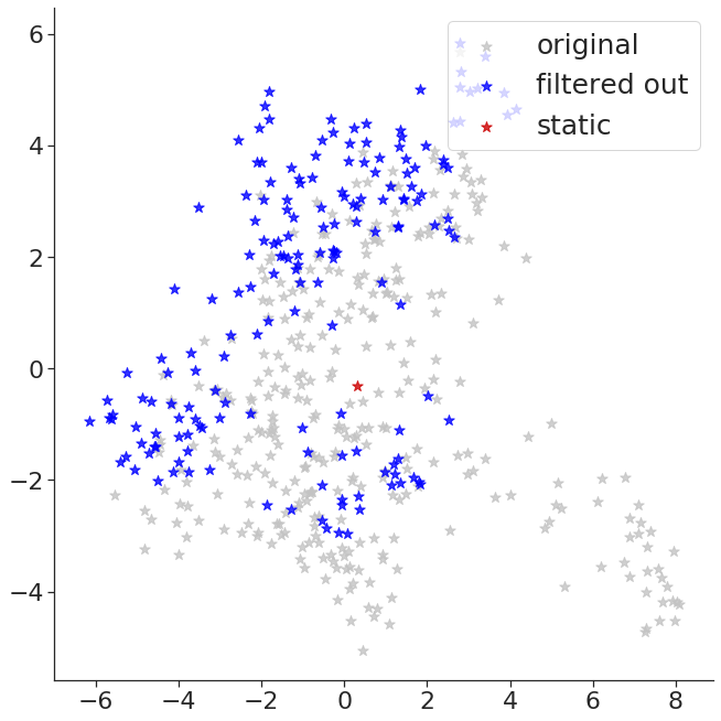
Qualitative analysis. Figures 3–17 show which mention vectors were filtered using the proposed strategy, for a number of different target words.

Figure 3: Plots of the mention vectors for ash, showing the mention vectors which are removed by the filtering strategy (blue) and the corresponding static vector (red).

Figure 4: Plots of the mention vectors for birch, showing the mention vectors which are removed by the filtering strategy (blue) and the corresponding static vector (red).

Figure 5: Plots of the mention vectors for bookcase, showing the mention vectors which are removed by the filtering strategy (blue) and the corresponding static vector (red).

Figure 6: Plots of the mention vectors for cicada, showing the mention vectors which are removed by the filtering strategy (blue) and the corresponding static vector (red).

Figure 7: Plots of the mention vectors for cockroach, showing the mention vectors which are removed by the filtering strategy (blue) and the corresponding static vector (red).

Figure 8: Plots of the mention vectors for cupboard, showing the mention vectors which are removed by the filtering strategy (blue) and the corresponding static vector (red).

Figure 9: Plots of the mention vectors for fridge, showing the mention vectors which are removed by the filtering strategy (blue) and the corresponding static vector (red).

Figure 10: Plots of the mention vectors for maggot, showing the mention vectors which are removed by the filtering strategy (blue) and the corresponding static vector (red).

Figure 11: Plots of the mention vectors for mantis, showing the mention vectors which are removed by the filtering strategy (blue) and the corresponding static vector (red).

Figure 12: Plots of the mention vectors for mosquito, showing the mention vectors which are removed by the filtering strategy (blue) and the corresponding static vector (red).

Figure 13: Plots of the mention vectors for palm, showing the mention vectors which are removed by the filtering strategy (blue) and the corresponding static vector (red).

Figure 14: Plots of the mention vectors for sapling, showing the mention vectors which are removed by the filtering strategy (blue) and the corresponding static vector (red).

Figure 15: Plots of the mention vectors for sofa, showing the mention vectors which are removed by the filtering strategy (blue) and the corresponding static vector (red).

Figure 16: Plots of the mention vectors for typewriter, showing the mention vectors which are removed by the filtering strategy (blue) and the corresponding static vector (red).

Figure 17: Plots of the mention vectors for willow, showing the mention vectors which are removed by the filtering strategy (blue) and the corresponding static vector (red).

Figure 18: Layer-wise performance on BabelNet domains (BERT).

Figure 19: Layer-wise performance on CSLB (BERT).

Figure 20: Layer-wise performance on Morrow (BERT).

Figure 21: Layer-wise performance on WordNet supersenses (BERT).

Figure 22: Layer-wise performance on X-McRae (BERT).

Figure 23: Layer-wise performance on BabelNet domains (RoBERTa).

Figure 24: Layer-wise performance on CSLB (RoBERTa).

Figure 25: Layer-wise performance on Morrow (RoBERTa).

Figure 26: Layer-wise performance on WordNet supersenses (RoBERTa).

Figure 27: Layer-wise performance on X-McRae (RoBERTa).

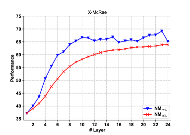
Layer	X-McRae		CSLB		Morrow		WordNet		BabelNet
	MAP	F1	MAP	F1	MAP	F1	MAP	F1	MAP	F1
1	56.8	60.0	58.7	63.4	57.5	62.6	35.1	41.0	32.3	39.0
2	56.7	59.9	59.3	64.4	60.3	65.8	37.1	41.2	34.6	40.8
3	59.5	61.3	60.0	65.1	64.7	69.2	38.9	43.5	34.9	41.8
4	60.4	62.4	61.1	65.9	66.2	68.3	40.0	44.5	34.9	42.7
5	63.0	64.3	61.9	66.6	70.8	71.2	41.9	45.8	35.7	43.0
6	65.5	66.7	63.1	68.0	72.2	74.6	44.6	48.0	37.2	43.6
7	65.8	67.8	63.0	68.1	73.3	74.1	45.2	48.2	38.2	44.1
8	65.7	67.3	62.1	67.5	74.2	74.0	45.5	48.9	38.9	44.8
9	67.1	68.4	62.6	67.9	74.7	74.5	45.1	48.7	38.8	44.4
10	66.6	68.9	61.6	66.8	72.8	74.0	43.6	47.0	38.0	45.2
11	65.6	67.3	61.2	66.5	72.3	72.0	43.3	47.3	37.6	44.0
12	66.0	67.0	60.9	66.4	71.2	71.1	43.1	46.8	36.4	43.4
13	65.8	67.0	60.5	65.9	70.3	70.3	42.6	46.8	37.3	43.6
14	67.1	68.2	60.4	65.8	71.2	70.8	42.6	46.8	37.2	43.4
15	67.3	67.9	61.1	66.5	72.5	72.1	42.9	47.0	37.9	43.8
16	67.2	67.9	61.3	66.5	72.4	72.0	43.0	47.6	37.5	43.6
17	67.3	67.7	60.7	66.3	71.5	71.3	43.3	47.3	36.9	43.3
18	67.1	68.3	61.2	67.0	72.8	73.4	44.3	48.0	36.9	43.5
19	67.5	68.8	61.3	66.7	73.0	73.2	44.5	48.1	38.1	43.7
20	67.8	69.2	61.5	66.7	71.2	71.2	44.1	47.7	37.3	42.9
21	68.3	70.0	62.1	67.3	72.8	73.4	44.8	48.3	38.5	43.1
22	68.9	70.3	62.5	67.4	73.5	72.2	44.4	47.3	38.7	43.5
23	68.6	69.4	62.0	66.8	70.2	70.7	43.6	46.4	37.1	42.2
24	67.8	68.3	61.7	66.3	70.5	69.9	41.6	45.2	37.2	42.4

Table 10: Results ($\%$) on validation set for classification tasks in each layer in terms of MAP and F1 scores, using mention vectors extracted from each layer of BERT.

Layer	X-McRae		CSLB		Morrow		WordNet		BabelNet
	MAP	F1	MAP	F1	MAP	F1	MAP	F1	MAP	F1
1	64.5	55.7	58.6	42.8	62.1	50.1	33.7	36.3	33.8	31.6
2	64.2	55.4	59.3	44.2	63.5	53.4	37.0	38.5	35.8	35.0
3	66.7	58.1	59.7	45.5	67.9	55.7	37.5	40.0	37.4	35.4
4	68.1	57.7	61.0	46.1	68.7	57.8	39.1	39.8	38.6	36.9
5	69.3	59.4	61.9	47.6	72.5	58.4	40.5	40.3	40.2	38.7
6	70.9	59.3	62.7	49.7	74.2	58.5	43.9	42.2	42.2	41.4
7	70.7	58.6	63.5	49.9	76.9	62.8	45.0	43.3	42.8	42.0
8	70.1	61.7	62.9	49.6	77.5	62.4	46.7	44.6	43.4	41.2
9	70.9	61.2	63.1	49.6	78.5	64.1	47.1	44.4	42.8	40.7
10	71.2	60.3	62.5	49.1	77.6	64.2	45.3	44.4	43.0	39.3
11	70.4	60.9	61.8	49.1	76.4	63.6	45.0	43.4	41.6	39.9
12	70.8	60.7	61.8	49.3	75.8	61.6	43.7	43.1	40.8	40.8
13	71.0	60.5	61.1	48.7	73.3	58.9	44.1	42.4	40.9	39.2
14	71.1	58.6	61.0	48.7	73.4	59.0	44.5	42.6	40.7	39.0
15	71.6	58.4	62.4	49.7	76.0	62.9	44.7	44.2	42.0	40.2
16	71.2	59.7	62.4	48.1	76.8	61.5	44.7	44.4	42.4	40.3
17	71.7	60.7	62.2	47.5	75.9	64.8	44.9	44.9	41.4	37.7
18	72.2	61.8	62.8	47.8	76.9	64.2	45.6	44.1	42.2	38.8
19	71.8	63.1	63.0	49.3	77.5	64.2	45.6	43.8	43.3	40.8
20	71.9	63.1	63.1	48.1	77.7	63.1	44.8	43.2	42.5	37.9
21	71.0	62.5	63.5	49.7	78.0	67.5	45.9	44.8	43.3	40.2
22	70.4	60.4	63.1	49.3	78.4	66.5	46.4	44.7	44.3	38.1
23	70.1	61.6	62.1	48.6	77.0	65.7	44.4	43.3	42.5	39.0
24	69.4	61.5	61.4	48.1	75.9	65.7	42.5	41.6	41.0	36.8

Table 11: Results ($\%$) on test set for classification tasks in each layer in terms of MAP and F1 scores, using mention vectors extracted from each layer of BERT.

Layer	X-McRae		CSLB		Morrow		WordNet		BabelNet
	MAP	F1	MAP	F1	MAP	F1	MAP	F1	MAP	F1
1	37.2	45.7	36.8	46.9	43.2	51.1	39.8	45.2	35.0	41.4
2	38.5	46.0	38.5	48.4	48.2	53.4	41.3	46.2	34.6	41.7
3	42.0	48.7	40.8	50.5	54.6	57.2	42.7	46.3	35.7	42.7
4	47.8	52.2	44.6	53.1	57.8	60.9	43.1	47.3	35.9	43.6
5	53.8	57.8	50.4	57.6	64.4	64.5	45.6	49.4	37.9	45.2
6	59.0	61.7	55.5	61.8	70.7	70.6	48.5	51.8	40.5	46.8
7	61.3	63.3	57.3	63.2	70.7	71.5	49.8	52.2	41.6	47.2
8	62.8	65.6	58.8	64.8	71.7	72.9	49.5	52.9	42.3	48.1
9	64.9	66.3	59.0	64.7	72.2	73.3	49.5	53.1	42.0	47.5
10	64.6	67.0	60.1	65.4	73.7	73.3	49.3	52.5	42.3	48.6
11	64.5	67.0	59.7	65.3	72.3	71.1	49.1	52.8	42.3	48.5
12	63.7	66.0	59.4	65.4	72.8	70.6	49.7	52.9	41.9	48.3
13	64.5	66.4	59.9	65.8	73.3	71.6	49.9	53.2	41.4	48.3
14	65.2	67.0	59.7	65.5	71.3	69.6	49.5	52.1	40.9	47.6
15	64.7	66.9	59.4	65.4	72.5	70.8	49.3	51.9	41.3	47.8
16	65.6	66.5	59.3	64.9	72.3	70.3	49.2	51.8	41.8	47.8
17	65.9	67.2	59.0	64.8	72.0	70.6	48.8	51.7	41.8	48.6
18	65.4	66.3	58.7	64.7	71.9	71.3	49.1	51.6	41.5	48.6
19	66.9	67.5	59.5	65.2	72.5	70.3	49.8	52.2	41.4	48.1
20	66.3	66.3	59.0	64.6	72.1	71.1	49.7	52.2	40.9	47.6
21	66.0	67.6	59.3	65.0	72.0	70.7	49.8	52.4	40.3	46.9
22	66.2	67.1	59.5	64.7	71.7	70.8	49.3	52.7	40.3	47.0
23	65.7	66.6	58.9	64.5	72.3	70.8	48.7	52.7	40.6	47.2
24	60.7	64.1	56.5	62.4	70.0	69.7	50.5	53.6	41.4	48.2

Table 12: Results ($\%$) on validation set for classification tasks in each layer in terms of MAP and F1 scores, using mention vectors extracted from each layer of RoBERTa.

Layer	X-McRae		CSLB		Morrow		WordNet		BabelNet
	MAP	F1	MAP	F1	MAP	F1	MAP	F1	MAP	F1
1	37.2	32.4	37.8	27.7	48.3	43.9	41.4	41.3	33.2	30.5
2	40.1	35.9	39.2	28.5	51.4	41.9	42.3	42.0	35.0	34.4
3	43.6	39.6	42.3	29.7	56.0	42.3	42.6	41.7	36.2	35.0
4	50.7	44.6	46.2	33.4	66.0	58.8	44.7	43.6	37.0	35.2
5	55.5	49.2	52.5	37.9	74.8	64.2	48.4	45.9	39.9	38.8
6	59.8	50.0	56.6	43.0	76.6	61.3	50.8	48.0	42.8	39.4
7	61.2	51.0	57.8	43.3	77.3	63.6	51.2	49.0	43.2	42.7
8	64.0	54.9	59.6	45.2	77.8	65.4	51.0	49.3	43.4	40.3
9	65.3	54.6	59.4	44.7	78.2	62.2	51.3	50.1	43.7	39.6
10	66.7	56.0	60.5	45.9	79.0	67.5	51.5	49.2	43.3	41.0
11	66.5	57.5	59.3	44.5	78.3	69.3	51.2	49.0	42.7	39.6
12	65.4	56.9	59.3	45.1	77.2	67.0	50.0	50.1	42.2	40.7
13	66.0	57.0	60.3	45.6	77.3	68.4	50.9	50.2	42.3	39.0
14	66.0	55.9	59.5	45.2	77.2	68.2	49.9	49.2	41.6	41.0
15	66.9	56.2	59.3	44.7	78.2	67.4	50.6	50.0	41.9	38.8
16	64.8	57.2	59.2	44.8	79.1	67.5	51.0	49.2	42.2	39.1
17	65.4	57.2	59.3	44.2	79.5	69.1	51.5	50.6	42.2	39.8
18	65.8	57.0	58.9	43.8	79.4	67.9	51.3	49.2	42.4	40.4
19	65.2	56.5	59.2	43.6	79.1	66.5	51.3	50.4	42.7	41.6
20	66.6	55.4	59.0	44.0	79.3	69.5	52.2	51.4	42.5	39.8
21	67.6	55.9	59.4	43.9	79.3	68.7	52.2	50.7	43.3	40.6
22	67.7	58.4	59.4	45.9	77.2	60.7	52.2	50.1	42.9	39.5
23	69.2	57.6	59.5	45.8	76.6	63.5	51.9	51.0	43.3	40.3
24	65.2	54.4	57.2	42.9	75.2	62.5	53.0	50.9	41.2	40.5

Table 13: Results ($\%$) on test set for classification tasks in each layer in terms of MAP and F1 scores, using mention vectors extracted from each layer of RoBERTa.

Layer	X-McRae		CSLB		Morrow		WordNet		BabelNet
	MAP	F1	MAP	F1	MAP	F1	MAP	F1	MAP	F1
1	56.8	60.0	58.7	63.4	57.5	62.6	35.1	41.0	32.3	39.0
2	57.0	59.5	59.0	64.1	59.3	65.0	36.5	41.6	33.7	40.3
3	57.6	60.1	59.7	64.6	61.6	66.1	37.3	42.1	33.9	40.7
4	58.7	60.9	60.0	64.8	63.4	67.5	37.9	42.2	34.3	41.2
5	59.5	61.3	60.7	65.3	64.1	68.9	39.2	43.2	34.7	42.0
6	60.8	62.5	61.5	66.1	66.4	69.8	40.9	44.8	35.3	42.5
7	62.1	63.9	61.8	66.6	69.2	70.2	42.1	45.9	35.6	42.6
8	63.1	64.8	62.2	67.0	70.8	71.6	43.2	46.6	36.1	43.1
9	63.6	65.7	62.4	67.3	72.1	72.4	43.6	47.0	36.9	43.2
10	64.1	65.8	62.7	67.5	72.8	72.7	44.2	47.1	37.1	43.3
11	64.4	66.1	62.8	67.6	73.4	72.8	44.5	47.3	37.3	43.4
12	64.6	66.0	62.5	67.4	74.0	73.1	44.7	47.4	37.5	43.7
13	64.5	66.1	62.4	67.2	73.9	72.6	45.0	47.6	37.7	43.8
14	64.9	66.4	62.5	67.3	74.3	73.4	45.2	47.6	37.8	43.9
15	65.2	66.5	62.6	67.3	74.7	74.2	45.4	47.7	37.6	43.9
16	65.6	66.6	62.7	67.4	75.2	74.0	45.4	48.2	37.8	44.1
17	66.0	66.5	62.6	67.4	75.3	74.0	45.4	48.4	37.9	44.2
18	65.9	66.7	62.5	67.4	75.3	74.6	45.3	48.5	37.8	43.7
19	66.2	67.0	62.7	67.6	75.5	74.6	45.3	48.7	37.7	43.6
20	66.4	67.1	62.7	67.7	74.9	74.5	45.3	48.8	37.9	43.7
21	66.6	67.3	62.7	67.6	75.2	74.5	45.5	49.1	38.1	43.8
22	67.1	68.1	62.7	67.7	75.1	74.5	45.6	49.2	38.2	43.7
23	67.2	68.3	62.8	67.8	75.3	75.0	45.7	49.2	37.9	43.8
24	67.2	68.3	62.9	67.9	75.4	75.2	45.8	49.3	37.9	43.8

Table 14: Results ($\%$) on validation set for classification tasks in terms of MAP and F1 scores, using mention vectors computed by averaging first $\ell$ layers, and extracted from BERT.

Layer	X-McRae		CSLB		Morrow		WordNet		BabelNet
	MAP	F1	MAP	F1	MAP	F1	MAP	F1	MAP	F1
1	64.5	55.7	58.6	42.8	62.1	50.1	33.7	36.3	33.8	31.6
2	64.3	54.9	58.9	44.2	62.4	50.8	34.9	37.2	35.0	34.7
3	65.1	57.1	59.3	44.7	65.5	51.2	36.2	38.6	35.2	34.9
4	66.2	57.2	59.7	44.4	66.0	53.9	37.0	38.5	36.0	35.3
5	67.2	57.8	60.2	45.4	67.7	56.9	38.9	39.4	37.4	35.1
6	68.2	58.0	61.5	45.8	69.8	58.2	40.1	40.3	38.8	35.4
7	68.9	60.2	62.4	47.0	72.4	61.0	41.0	41.8	39.5	36.6
8	69.2	59.4	62.7	47.9	74.0	60.3	42.0	42.2	40.4	37.7
9	69.4	60.2	62.8	47.9	74.8	62.8	42.8	42.6	41.3	40.3
10	70.0	59.1	62.9	48.4	75.3	62.7	43.1	42.7	41.4	39.8
11	69.9	58.4	62.9	48.3	75.5	63.7	43.6	43.1	41.6	40.3
12	70.1	58.3	62.9	48.7	75.8	64.2	44.0	43.1	41.6	39.7
13	70.1	58.7	62.9	48.7	75.7	62.5	44.4	42.5	41.9	39.8
14	70.2	59.3	62.9	49.3	75.7	61.6	44.7	44.0	41.6	40.5
15	70.2	59.7	63.2	48.9	75.6	61.6	45.0	44.0	41.8	40.4
16	70.4	60.0	63.1	49.5	75.9	63.8	45.5	43.5	41.8	40.5
17	70.4	59.4	63.2	49.5	75.9	63.1	45.8	42.8	41.9	40.1
18	70.1	59.6	63.2	49.1	75.7	62.7	45.9	43.0	42.2	40.8
19	69.9	59.7	63.1	49.6	75.9	62.5	46.0	43.0	42.2	40.5
20	70.1	60.3	63.2	49.4	75.4	62.2	46.2	44.1	42.3	40.2
21	70.2	60.5	63.4	49.1	75.1	62.4	46.2	43.9	42.6	40.6
22	70.4	60.5	63.3	49.4	75.3	63.0	46.4	44.7	42.6	40.5
23	70.5	60.7	63.3	49.1	75.8	63.4	46.5	44.9	42.3	40.9
24	70.6	60.9	63.3	48.8	76.4	62.9	46.6	44.8	42.2	41.0

Table 15: Results ($\%$) on test set for classification tasks in terms of MAP and F1 scores, using mention vectors computed by averaging first $\ell$ layers, and extracted from BERT.

Layer	X-McRae		CSLB		Morrow		WordNet		BabelNet
	MAP	F1	MAP	F1	MAP	F1	MAP	F1	MAP	F1
1	37.2	45.7	36.8	46.9	43.2	51.1	39.8	45.2	35.0	41.4
2	37.9	45.9	38.0	47.9	46.7	53.1	40.6	45.9	35.6	41.0
3	40.1	47.1	39.0	48.8	50.8	54.4	42.0	46.1	35.9	41.7
4	43.0	49.6	40.9	50.2	53.9	56.2	43.1	47.0	36.0	42.6
5	46.8	51.9	43.4	52.2	57.0	59.9	44.5	48.3	36.8	43.7
6	49.7	54.0	46.0	54.2	60.8	62.2	45.9	49.5	37.6	44.3
7	52.5	55.9	48.2	55.8	63.1	64.4	46.5	50.5	38.7	45.0
8	54.9	57.2	50.4	57.5	65.6	66.0	47.1	51.1	39.5	45.6
9	57.1	59.6	52.3	58.9	67.5	66.8	47.4	51.3	39.9	46.3
10	58.4	60.5	53.4	60.1	68.7	68.2	47.9	51.7	40.3	46.5
11	59.7	61.5	54.4	61.0	69.3	68.8	48.2	52.1	40.6	46.9
12	60.3	61.9	55.2	61.7	70.0	69.7	48.7	52.6	40.8	47.0
13	60.7	62.2	55.9	62.4	70.1	70.3	48.9	52.8	41.3	47.2
14	61.5	62.6	56.7	62.8	70.7	70.3	49.1	52.8	41.3	47.4
15	61.4	62.9	57.1	63.2	72.5	70.8	49.2	53.0	41.6	47.4
16	61.7	63.4	57.3	63.5	71.8	70.1	49.4	52.9	41.6	47.6
17	62.0	63.8	57.6	63.7	72.1	70.0	49.5	53.1	41.8	47.6
18	62.2	64.3	58.0	63.9	72.4	70.9	49.6	53.1	41.6	47.6
19	62.7	64.9	58.2	64.1	72.3	70.9	49.6	53.0	41.6	47.7
20	63.1	65.4	58.0	64.2	72.4	70.9	49.6	52.9	41.6	47.7
21	63.3	65.7	58.2	64.4	72.4	71.1	49.6	52.8	41.5	47.8
22	63.5	66.0	58.3	64.5	72.7	70.7	49.6	52.7	41.4	47.9
23	63.6	66.0	58.4	64.5	73.7	71.6	49.7	52.9	41.4	47.7
24	63.5	66.0	58.5	64.5	73.8	71.9	49.7	53.0	41.4	47.7

Table 16: Results ($\%$) on validation set for classification tasks in terms of MAP and F1 scores, using mention vectors computed by averaging first $\ell$ layers, and extracted from RoBERTa.

Layer	X-McRae		CSLB		Morrow		WordNet		BabelNet
	MAP	F1	MAP	F1	MAP	F1	MAP	F1	MAP	F1
1	37.2	32.4	37.8	27.7	48.3	43.9	41.4	41.3	33.2	30.5
2	39.0	34.8	38.4	28.2	49.1	43.7	41.3	42.1	34.3	33.0
3	41.0	37.3	40.2	29.3	51.7	40.9	41.6	41.7	35.0	35.0
4	43.8	38.9	41.6	29.8	56.3	46.5	42.8	43.0	36.3	34.6
5	47.6	43.5	44.4	32.3	64.1	51.4	45.1	44.5	37.4	33.3
6	50.6	45.4	47.9	34.2	67.5	56.1	46.9	44.0	38.8	35.6
7	53.4	46.9	50.1	35.7	72.5	59.0	48.6	46.8	40.4	36.0
8	55.4	47.3	52.2	37.0	74.3	58.8	49.6	47.8	41.2	38.0
9	57.1	50.2	53.6	39.2	75.6	61.1	50.1	47.9	41.9	38.6
10	58.2	51.5	55.0	40.3	76.2	61.5	50.7	49.2	42.4	39.5
11	59.2	52.6	55.9	40.8	77.1	60.5	51.1	49.1	42.6	39.9
12	60.1	51.9	56.5	41.2	77.4	61.1	51.2	49.5	42.8	38.7
13	60.8	52.4	57.0	41.4	77.5	63.8	51.5	50.3	43.1	39.6
14	61.4	53.6	57.5	42.1	77.7	64.5	51.6	49.7	43.0	39.5
15	61.8	53.5	57.8	42.1	77.6	65.0	51.1	49.6	43.1	39.7
16	61.9	54.3	58.1	42.0	77.6	64.9	51.6	49.8	43.3	39.2
17	62.3	54.0	58.2	42.5	77.8	66.7	51.5	50.0	43.1	39.2
18	62.8	54.0	58.3	42.4	77.7	67.2	51.6	50.2	42.9	38.9
19	63.0	53.0	58.5	42.5	77.6	68.5	51.7	50.1	42.9	40.1
20	63.0	53.2	58.7	42.5	77.9	67.8	51.6	49.4	43.1	40.0
21	63.2	53.8	58.7	43.1	78.0	67.2	51.6	49.6	43.2	39.3
22	63.4	53.3	58.7	43.5	77.9	67.4	51.3	49.7	43.3	39.3
23	63.9	53.6	59.0	43.9	77.9	67.5	51.3	50.2	43.4	39.0
24	63.9	53.5	58.9	44.2	77.9	67.5	51.3	49.8	43.2	38.7

Table 17: Results ($\%$) on test set for classification tasks in terms of MAP and F1 scores, using mention vectors computed by averaging first $\ell$ layers, and extracted from RoBERTa.

References

- Agirre et al. [2009] Eneko Agirre, Enrique Alfonseca, Keith Hall, Jana Kravalova, Marius Paşca, and Aitor Soroa. A study on similarity and relatedness using distributional and WordNet-based approaches. In Proceedings of NAACL, pages 19–27, 2009.
- Amrami and Goldberg [2019] Asaf Amrami and Yoav Goldberg. Towards better substitution-based word sense induction. arXiv:1905.12598, 2019.
- Bommasani et al. [2020] Rishi Bommasani, Kelly Davis, and Claire Cardie. Interpreting pretrained contextualized representations via reductions to static embeddings. In Proceedings ACL, pages 4758–4781, 2020.
- Bruni et al. [2014] Elia Bruni, Nam-Khanh Tran, and Marco Baroni. Multimodal distributional semantics. J. Artif. Intell. Res., 49(1-47), 2014.
- Camacho-Collados and Navigli [2017] Jose Camacho-Collados and Roberto Navigli. BabelDomains: Large-scale domain labeling of lexical resources. In Proc. EACL, pages 223–228, 2017.
- Camacho-Collados et al. [2017] Jose Camacho-Collados, Mohammad Taher Pilehvar, Nigel Collier, and Roberto Navigli. SemEval-2017 task 2: Multilingual and cross-lingual semantic word similarity. In Proc. SemEval, pages 15–26, 2017.
- Ciaramita and Johnson [2003] Massimiliano Ciaramita and Mark Johnson. Supersense tagging of unknown nouns in WordNet. In Proc. EMNLP, pages 168–175, 2003.
- Das et al. [2015] Rajarshi Das, Manzil Zaheer, and Chris Dyer. Gaussian LDA for topic models with word embeddings. In Proc. ACL, pages 795–804, 2015.
- Devlin et al. [2019] Jacob Devlin, Ming-Wei Chang, Kenton Lee, and Kristina Toutanova. BERT: pre-training of deep bidirectional transformers for language understanding. In Proc. NAACL-HLT, 2019.
- Ethayarajh [2019] Kawin Ethayarajh. How contextual are contextualized word representations? comparing the geometry of BERT, ELMo, and GPT-2 embeddings. In Proc. EMNLP, pages 55–65, 2019.
- Finkelstein et al. [2002] Lev Finkelstein, Gabrilovich Evgenly, Matias Yossi, Rivlin Ehud, Solan Zach, Wolfman Gadi, and Ruppin Eytan. Placing search in context: The concept revisited. ACM Transactions on Information Systems, 20(1):116–131, 2002.
- Forbes et al. [2019] Maxwell Forbes, Ari Holtzman, and Yejin Choi. Do neural language representations learn physical commonsense? Proc. CogSci, 2019.
- Hill et al. [2015] Felix Hill, Roi Reichart, and Anna Korhonen. SimLex-999: Evaluating semantic models with (genuine) similarity estimation. Computational Linguistics, 41(4):665–695, 2015.
- Kolyvakis et al. [2018] Prodromos Kolyvakis, Alexandros Kalousis, and Dimitris Kiritsis. Deepalignment: Unsupervised ontology matching with refined word vectors. In Proc. NAACL-HLT, pages 787–798, 2018.
- Li et al. [2019] Na Li, Zied Bouraoui, and Steven Schockaert. Ontology completion using graph convolutional networks. In Proc. ISWC, pages 435–452, 2019.
- Liu et al. [2019] Yinhan Liu, Myle Ott, Naman Goyal, Jingfei Du, Mandar Joshi, Danqi Chen, Omer Levy, Mike Lewis, Luke Zettlemoyer, and Veselin Stoyanov. RoBERTa: A robustly optimized BERT pretraining approach. CoRR, abs/1907.11692, 2019.
- Ma et al. [2016] Yukun Ma, Erik Cambria, and Sa Gao. Label embedding for zero-shot fine-grained named entity typing. In Proc. COLING, pages 171–180, 2016.
- McRae et al. [2005] Ken McRae et al. Semantic feature production norms for a large set of living and nonliving things. Behavior research methods, 37:547–559, 2005.
- Mickus et al. [2019] Timothee Mickus, Denis Paperno, Mathieu Constant, and Kees van Deemeter. What do you mean, BERT? assessing BERT as a distributional semantics model. arXiv:1911.05758, 2019.
- Mikolov et al. [2013] Tomas Mikolov, Kai Chen, Greg Corrado, and Jeffrey Dean. Efficient estimation of word representations in vector space. In Proc. ICLR, 2013.
- Morrow and Duffy [2005] Lorna I Morrow and M Frances Duffy. The representation of ontological category concepts as affected by healthy aging: Normative data and theoretical implications. Behavior research methods, 37(4):608–625, 2005.
- Onal et al. [2018] Kezban Dilek Onal, Ye Zhang, Ismail Sengor Altingovde, Md Mustafizur Rahman, Pinar Karagoz, Alex Braylan, Brandon Dang, Heng-Lu Chang, Henna Kim, Quinten McNamara, et al. Neural information retrieval: At the end of the early years. Information Retrieval Journal, 21(2-3):111–182, 2018.
- Pennington et al. [2014] Jeffrey Pennington, Richard Socher, and Christopher D. Manning. GloVe: Global vectors for word representation. In Proc. EMNLP, pages 1532–1543, 2014.
- Rubenstein and Goodenough [1965] Herbert Rubenstein and John B. Goodenough. Contextual correlates of synonymy. Communications of the ACM, 8(10):627–633, 1965.
- Socher et al. [2013] Richard Socher, Milind Ganjoo, Christopher D Manning, and Andrew Ng. Zero-shot learning through cross-modal transfer. In Proc. NIPS, pages 935–943, 2013.
- Vimercati et al. [2019] Manuel Vimercati, Federico Bianchi, Mauricio Soto, and Matteo Palmonari. Mapping lexical knowledge to distributed models for ontology concept invention. In Proc. IA*AI, pages 572–587, 2019.
- Vulic et al. [2020] Ivan Vulic, Edoardo Maria Ponti, Robert Litschko, Goran Glavas, and Anna Korhonen. Probing pretrained language models for lexical semantics. In Proceedings EMNLP, pages 7222–7240, 2020.
- Weir et al. [2020] Nathaniel Weir, Adam Poliak, and Benjamin Van Durme. On the existence of tacit assumptions in contextualized language models. arXiv:2004.04877, 2020.